regional trade openness index, income disparity and … · 5.3 relation between openness and pcnsdp...
TRANSCRIPT

#0807
Regional Trade Openness Index,Income Disparity and Poverty
- An Experiment with Indian Data
Regional Trade Openness Index,Income Disparity and Poverty
- An Experiment with Indian Data
Regional Trade Openness Index,Income Disparity and Poverty
- An Experiment with Indian Data
Regional Trade Openness Index,Income Disparity and Poverty- An Experiment with Indian Data
Published by
D-217, Bhaskar Marg, Bani ParkJaipur 302 016, IndiaTel: +91.141.228 2821, Fax: +91.141.228 2485Email: [email protected] site: www.cuts-international.org
Written by
Sugata Marjit* and Saibal Kar**
With the support of
Printed byJaipur Printers P. Ltd.Jaipur 302 001
ISBN: 978-81-8257-102-0
© CUTS International, 2008
This volume has been produced with the financial assistance of Royal Norwegian Embassy,New Delhi under the project entitled, “Mainstreaming International Trade into National Develop-ment Strategy: A Pilot Project in Bangladesh and India”. The views expressed herein are thoseof the authors and can therefore in no way be taken to reflect the positions of CUTS International,the Royal Norwegian Embassy, New Delhi and the institutions with which the authors are affiliated.
* Director and RBI Professor of Industrial Economics, Centre for Studies in Social Sciences,Calcutta, (CSSSC), India. Email: [email protected]
** Associate Professor of Economics, Centre for Studies in Social Sciences, Calcutta(CSSSC), India. Email: [email protected]
#0807, Suggested Contribution: Rs.200/US$20
Royal NorwegianEmbassy,New Delhi

Table of Contents
List of Tables ............................................................................................................... i
List of Figures ............................................................................................................. ii
Acronyms .................................................................................................................. iii
Executive Summary.................................................................................................... iv
I. Introduction ......................................................................................................... 1
2. Review of Literature............................................................................................ 32.1 Economic Reforms and Poverty in India .................................................... 32.2 Economic Reforms and Formal Employment in India................................. 62.3 Economic Reforms and Regional Disparity in India ................................... 7
3. Theoretical Background................................................................................... 12
4. Data, Methodology and Results......................................................................... 14
5. Relationship between Openness and Inter-regional Income Disparity............ 285.1 Relation between Openness and PCNSDP of the States ......................... 295.2 Relation between Openness and Dispersion of PCNSDP ........................ 335.3 Relation between Openness and PCNSDP Growth of the States ............. 34
6. Openness Index and Industrial Jobs................................................................. 39
7. Openness Index and Poverty across States in India.......................................... 44
8. Concluding Remarks........................................................................................ 48
References ................................................................................................................ 49
Annexure ................................................................................................................. 53
Appendix ................................................................................................................. 58
List of Tables
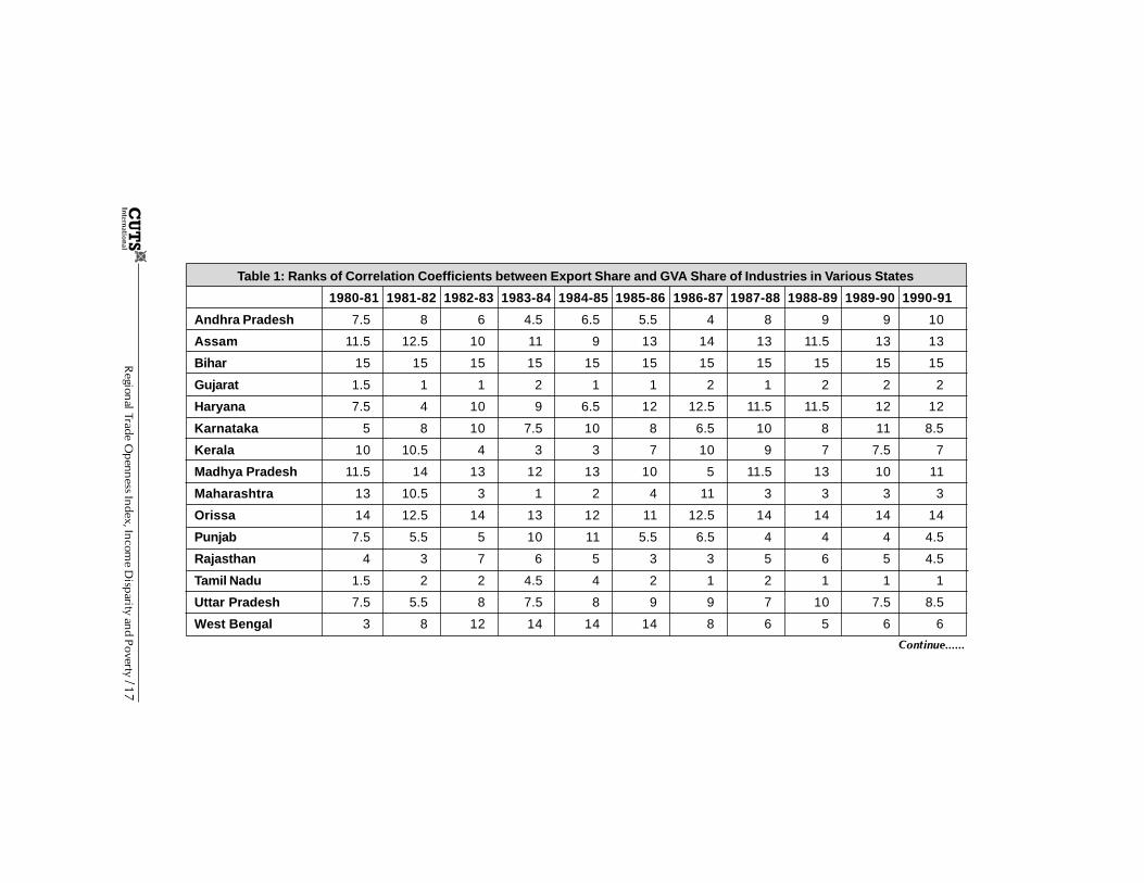
Table 1: Ranks of Correlation Coefficients between ExportShare and GVA Share of Industries in Various States ............................... 17
Table 2: Ranks of Correlation Coefficients between Import Share andGVA Share of Industries in Various States ................................................ 19
Table 3: Inverse Ranks of Correlation Coefficients between ImportShare and GVA Share of Industries in Various States ............................... 21
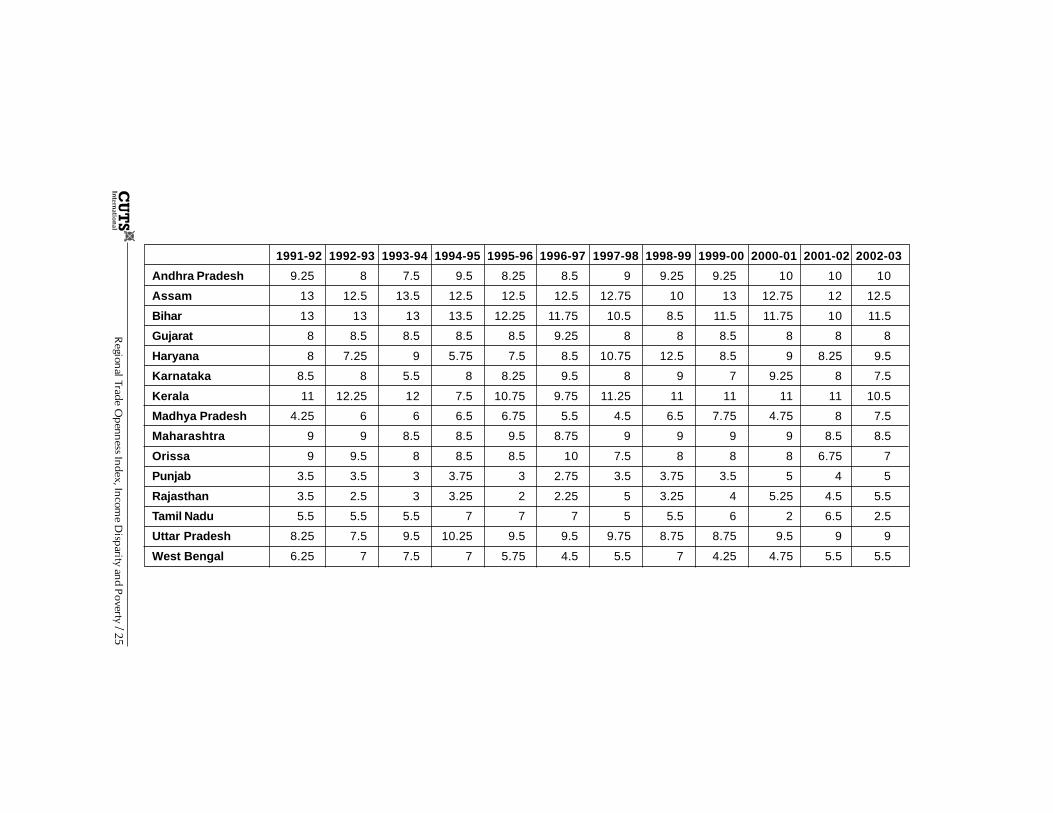
Table 4: Yearly Openness Index Values of Indian States ........................................ 24
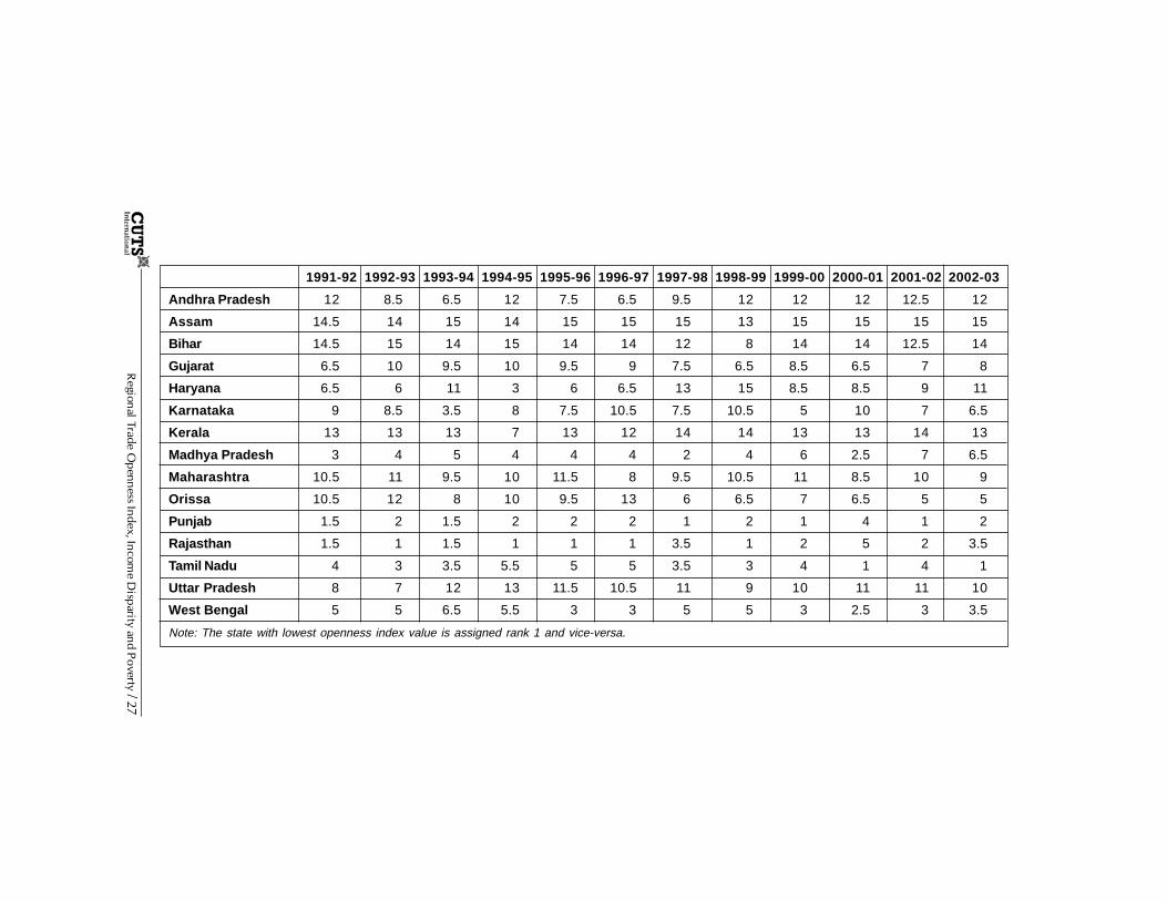
Table 5: Yearly Openness Index Ranks of Indian States ........................................ 26
Table 6: Coefficient of Variation of PCNSDP across major States in India ............. 29
Table 7: Ranks of States According to PCNSDP .................................................... 30
Table 8: Rank of States on Relative Mean Deviation of States’ Income ................. 36
Table 9: Rank of States on Growth Rate of PCNSDP .............................................. 38
Table 10: Correlation between Growth of Workers and TOI across Industries ........ 40
Table 11: Correlation between TOI and Growth of Employees acrossIndustries (SIC) ......................................................................................... 41
Table 12: Correlation between TOI and Urban and Rural HCR, Urbanand Rural PG, Urban and Rural SPG and Urban and Rural GINI ................ 45
Regional Trade Openness Index, Income Disparity and Poverty / i

List of Figures
Figure 1: Trend of Coefficient of Variation of PCNSDPacross major States in India, 1980-81 to 2002-03 .................................... 28
Figure 2: Correlation Coefficients and Trend Line between ExportPerformance and PCNSDP Ranks across States (1980-81 to 2002-03) .... 32
Figure 3: Correlation Coefficients and Trend Line between Import CompetingPerformance and PCNSDP Ranks across States (1980-81 to 2002-03) .... 32
Figure 4: Correlation Coefficients and Trend Line between OpennessIndex and PCNSDP Ranks across States (1980-81 to 2002-03) .............. 33
Figure 5: Correlation Coefficient between Openness Index Rank & Rank ofRelative Mean Deviation based on PCNSDP (1980-82 to 2002-03) ......... 34
Figure 6: Correlation Coefficient between Rank of PCNSDP Growth &Rank of Openness Index (1981-82 to 2002-03)........................................ 36
Figure 7: Correlation between Regional TOI and Growthof Workers across Industries (SIC) ........................................................ 42
Figure 8: Correlation between Regional TOI and Growth ofEmployees across Industries (SIC) ........................................................ 42
Figure 9: Correlation Coefficient between Growth Rate ofWorkers and TOI for SIC 20-21 .............................................................. 43
Figure 10: Correlation Coefficient between Growth Rate ofEmployees and TOI for SIC 20-21.......................................................... 43
Figure 11: Correlation Coefficient between Urban and Rural HCR and TOI ........... 45
Figure 12: Correlation Coefficient between TOI andUrban and Rural Poverty Gap ................................................................ 46
Figure 13: Correlation Coefficient between TOI and Urban andRural Squared Poverty Gap .................................................................... 47
Figure 14: Correlation Coefficient between TOI and Urban and Rural Gini ............ 47
ii / Regional Trade Openness Index, Income Disparity and Poverty

Regional Trade Openness Index, Income Disparity and Poverty / iii
Acronyms
ASI Annual Survey of Industries
CSOs Civil Society Organisations
DGCI&S Directorate General of Commercial Intelligence and Statistics
EU European Union
GDP Gross Domestic Product
GVA Gross Value Added
HCR Head Count Ratio
HDI Human Development Index
NAFTA North American Free Trade Agreement
NIC National Industrial Classification
NSDP Net State Domestic Product
PCNSDP Real Per Capita Net State Domestic Product
PGI Poverty Gap Index
PPP Purchasing Power Parity
SCs Schedule Castes
SDP State Domestic Products
SPGI Squared Poverty Gap Index
STs Schedule Tribes
TFP Total Factor Productivity
TFPG Total Factor Productivity Growth
TOI Trade Openness Index
Executive Summary
This study, “Mainstreaming International Trade into National Development Strategy:A Pilot Project in Bangladesh and India”, aims to examine how ‘open’ Indian
states are with respect to international trade and uses the index of regional opennessthus constructed to reflect on several aspects that affect the level of poverty in India,directly and indirectly. In this connection it should be noted that the estimation of thedegree of openness is done for each state vis-à-vis rest of the world and not ‘between’states in India, since it was difficult to have access to inter-state trade data. This meansthat even if one of the states produces an important intermediate commodity and anotherstate processes it in favour of manufacturing an export commodity, the latter should bedeemed more open to external trade as compared to the former.
Tracing the vertical (and in cases, horizontal) linkages in production and trade maytherefore provides another possible method of capturing the degree of openness foreach state vis-à-vis world trade. The construction of the present regional opennessindex within the geographic boundaries of a nation state is novel in the economicliterature, and applications of this index in the Indian context provides new insights intoseveral issues in growth and development, which has not been attempted so far.
Albeit the starting point in this analysis is the construction of the openness index asbriefly described above, the main focus is in providing an account of the trade-povertylinkage in the Indian context. The poverty issue is in itself a subject of infinite interestand the purpose here is to evaluate the poverty situations in different states in Indiabetween 1980 and 2003 with the aid of the openness index. The broad purpose is toobserve if state level trade openness, in the manner the concept is developed in thisstudy, has any implications for the corresponding levels of poverty.
A major contribution of this project has been to construct and refine the index of regionalor state-specific openness index in India typically because it is well known thatinternational trade data for sub-national levels is not available. This is particularly aproblem for countries that are large in size and have heterogeneous regions. Thus astarting hypothesis is the fact that opening up to international trade affects differentregions within the same country disparately, depending upon their production matrix. Inthe absence of state level trade data, the study devises a proxy index, which allows it torank states over time in terms of their exposure to trade. This index is potentially timevariant and therefore is amenable to time series analytics. It is observed that the relativeincome of a region is closely related to the extent of openness and that such relationshipgets stronger over time. It demonstrate that trade openness has contributed significantlyto divergent income patterns across states in India.
iv / Regional Trade Openness Index, Income Disparity and Poverty
The aftermath of trade liberalisation in India provides an ideal ground for applying thesethoughtful experiments to practice with a focus on the three delicately inter-linkedissues: the state of inter-regional disparity; the evolving employment patterns acrossindustries; and the state level poverty dynamics. However, for the sake ofcomprehensiveness, the study dwells upon the evidence starting from 1980s, leavingample ground for any relevant comparison between the pre- and post-reform years. Theunifying thread between the first two issues, other than the openness index acting as afacilitator for all three, is the industrial classifications of different commodities producedin India and the changes at the industrial level – both in terms of output and employment.The methodology developed for this study is fairly general and may find similarapplications in countries other than India.
Regional Trade Openness Index, Income Disparity and Poverty / v

Regional Trade Openness Index, Income Disparity and Poverty / 1
1 Introduction
Traditional trade theories argue that the removal of trade barriers have impact on theindustrial dynamics of a country depending on the factor intensities of these
industries. As a country engages more and more in international trade, its factors ofproduction will enter increasingly into the export sector, where their return is higher,compared to the import competing sector. The same thing can be envisaged at theregional level. Consequently, the states, which can attune their production structure tointernational demands, should earn higher than other states. Hence, the relative incomeof a region depends on the extent of openness to trade.
This study aims to examine how much ‘open’ Indian states are with respect to internationaltrade and then assesses to characterise three related aspects: (1) trade openness andincidence, depth and severity of poverty at the state level (rural and urban); tradeopenness and income inequality at the state level (rural and urban); (2) trade opennessand industrial employment across industry types (workers and employees); and (3)trade openness and regional disparity. It should be noted that this study focuses primarilyon finding the inter-linkage between trade openness at the state level and its implicationsfor poverty. However, the precursor for this and other related issues is the constructionof trade openness index on which a substantial portion of the study is devoted.
Thus, construction of a workable openness index at the regional or state level becomesrather demanding since it is well recognised that international trade data are not easilyavailable at the sub-national level. This is particularly a problem for countries that arelarge in size and have diverse heterogeneous regions. The methodology developed forthis study is not only applicable to the Indian scenario but should also be useful formany countries where state level trade data are not available. The study devises a proxy,which allows it to rank states over time in terms of their exposure to trade. In otherwords, the level of openness existing in each state stands vis-à-vis the rest of the worldand not in comparison to another state within the same nation.
Though the study discusses the effects of trade openness on poverty, inequality andemployment at length, there is need to justify why it takes up the issue on regionaldisparity basis. For geographically large developing countries having disparate regions,it is essential to understand whether trade has an equalising impact or not. Unfortunately,there are not many papers that deal with intra-national inequality as dictated by thevolume and nature of international trade. Available work on European Union (EU) where
2 / Regional Trade Openness Index, Income Disparity and Poverty
countries are treated as regions is not as problematic as the one this study deals with,since in EU trade data is readily available for each nation.
The closest paper related to this study and dealing with the EU is by Egger, Huber andPfaffermayr (2005), which extends the empirical literature on the effects of tradeliberalisation on regional disparities within a country. In their study on the case of theCentral and Eastern European countries, the authors found significant convergence ofreal wages in Poland and Bulgaria only. Furthermore, countries with faster growingexport openness in the period 1991 experienced larger increases in their regionaldisparities. Despite apparent similarity with the issue in the present study, it should benoted that this paper does not use intra-national trade data, which consequently allowssubstantial differences in both idea and approach as developed here.
This study essentially focuses on the case where sub-national database is invoked toshed light on the state of regional disparity within the country in question. The sub-national openness index is used to find some relationship with inter-state variations inincome – both at levels and as percentage changes. While the study does not intend todo any causality analysis, it aims to build up a case for such an analysis by looking atthe correlation between an analytically constructed index and state level income measures.
This study is structured in a following manner while section I introduces the study,Section 2 provides a coherent literature survey on the close connections betweeneconomic or trade reform and poverty in India on trade and employment and finally ontrade and regional disparity. Section 3 discusses two theoretical papers, which providethe backbone to the statistical methodology devised in this paper. Section 4 providesthe data, detailed methodology and the openness index. Section 5 examines therelationship between the index and inter-regional income disparity. Section 6 discussesthe use of regional Trade Openness Index (TOI) on observing growth of industrial jobsclassified by industrial categories. Section 7 deals with the focal issue, i.e. the relationshipbetween TOI and various estimates of poverty and inequality, while Section 8 providesconclusion.

Regional Trade Openness Index, Income Disparity and Poverty / 3
2Review of Literature
2.1 Economic Reforms and Poverty in IndiaDebates loomed large throughout the post-independence decades regarding themeasures to capture the incidence and depth of income poverty in India and the policiesmost appropriate in lowering them thus measured. While the discourse reached someconsensus in identifying the problems and the possible cures, however ambitious, theonset of the economic reforms in the early 1990s added a completely new dimension tothe entire debate. The reforms clearly marked an important watershed in the economichistory of the country, and which proliferated renewed interests in measuring povertyand inequality in the post-reform era. And yet, the causality between ‘trade openness’ inIndia and the measures of poverty seems relatively under-explored except for a fewreliable studies produced in recent times.
High rates of gross domestic product (GDP) growth in the recent years have encouragedeconomists and policy makers to explore whether such growth has contributed to thereduction in poverty across states. Although rates of poverty in urban and rural areashave shown declining trends in general, the outcome varies considerably across states.Topalova (2005) argues that tariff reduction on importable commodities has not beeneffective in reducing the incidence and depth of poverty across districts in India withconcentration of import-competing activities. Using a specific factor model of trade thestudy shows that in the presence of limited factor mobility, trade liberalisation caused toincrease the extent of rural poverty in India. However, the increase in rural poverty wasless striking in states that had more flexible labour market institutions. In a similar vein(also considering product and labour market deregulations) and in connection with theeffect of trade on poverty in India, Hasan, Mitra and Ural (2006) provide contradictoryevidence to the impact of trade reform on poverty which is actually shown more visiblein states with relatively ‘flexible’ labour market conditions.
Moreover, this is consistent with the position of Besley and Burgess (2004) thoughflexible labour market characteristics do have some exceptions. According to their results,Maharastra and Gujarat despite being not so flexible in terms of the conditions set out inthis paper have shown impressive improvements. But more generally, studies on povertyin India categorically speak of various measures of poverty, of the connection betweeneconomic growth and poverty, of redistribution and poverty, of poverty and inequalityand more recently – as this survey focuses on – of economic reforms and poverty. Since
4 / Regional Trade Openness Index, Income Disparity and Poverty
the existing literature on each of these areas is extensive, the study would bypass all infavour of concentrating exclusively on the economic reforms and poverty related issues.
There is little doubt that the economic reforms since early 1990s have had significantimpacts on the income and poverty levels in both rural and urban India. A number ofrecent empirical studies show that the percentage of poverty has declined both at theall-India and regional (States/UTs) levels.1The causes underlying such changes arediverse. Not surprisingly, the evolving relationships between poverty and inequalitytoo have numerous interpretations, of which a notable contribution is available in Drezeand Sen (2002). Using an international poverty line of around US$1 per day at 1993Purchasing Power Parity (PPP), it is estimated that about one third of the poor in the mid-1990s lived in India (Datt and Ravallion, 2002a). Therefore, what happens to the incidenceof absolute poverty in India is quantitatively important to the world’s overall progress infighting absolute poverty.
In India, the decadal average growth rates for 1960s and 1970s were around 3.4 percent,implying per capita growth rates of about one percent. The growth rates in nationaloutput since the mid-1980s and in particular since 1993 have been appreciably higher onaverage than in the 1960s and 1970s. The growth rate in net national product per capitawas 4.8 percent per annum between 1993-94 and 1999-00. It is widely believed that thereforms of the 1990s were instrumental in achieving higher growth. However, it is notclear how much India’s poor have shared in those gains.
Before focusing on the 1990s and to the connection between economic reforms andpoverty, a quick glance on the broader trends of growth rates and the incidence ofpoverty between 1960-2000, as presented in Datt and Ravallion (2002a, Table 1) seemsrelevant. They show that the poverty level has gone down considerably although thestagnation in the rural poverty level has in fact increased the rural-urban poverty ratioduring these years. While this may be considered as a partisan look at the larger debate,other notions that also prevail strong are considered next. Essentially, a survey of someof the existing studies is meant to see if a consensus emerges regarding the directionand magnitude of changes in poverty as well as inequality estimates in the 1990s and theextent to which such changes can be attributed to the major policy elements of reformsin India.2
In fact, the general picture in the 1990s was quite contentious. This stands firmly incontrast to the broader consensus prevailing in the 1980s that poverty rates had fallenappreciably during the decade. In general, two visibly polar notions about the impact ofreform on poverty dominate the literature, although there are also some studies that donot find clear evidence on the influence of economic reforms on poverty. One groupstrongly claims that poverty reduction in India in the decade of the 1990s have beensummarily dismal. This group includes Ninan (1994, 2000), Dev (1995), Tendulkar andJain (1995), Tendulkar and Jain (1995) and others. Ninan (2000) provides a re-estimate(following an initial estimate in 1994) of rural, urban and national level poverty trends inIndia.
It is claimed that, while rural, urban and overall national poverty levels in India recordeda significant decline during the pre-reform periods (1969-70 to 1990-91), during the post-

Regional Trade Openness Index, Income Disparity and Poverty / 5
reform period (1991-92 to 1993-94), these negative trends have weakened or got reversedin terms of one or more poverty indicators – namely, Head Count Ratio (HCR), PovertyGap Index (PGI) or Squared Poverty Gap Index (SPGI). Furthermore, majority of the 15larger states in India that contributed positively towards overall poverty reduction inthe pre-reform decades reported statistically insignificant poverty reduction rates in thepost-reform period – Punjab and Haryana even reporting an actual increase in ruralpoverty.
A few other contemporary studies (Dev, 1995; Gupta, 1995; Tendulkar and Jain, 1995 andothers), which might have been somewhat pre-mature in assessing the role of economicreforms on poverty, also note increases in both rural and urban poverty rates. Dev(1995) reports an increase in poverty rates during the ‘first 18 months’, after economicreforms were initiated in India. Tendulkar and Jain (1995) claim a sharp increase in ruralpoverty rates with a moderate rise in urban poverty rates during 1991-95, although thereforms were only ‘indirectly’ responsible for such a trend. Gupta (1995) believes thatthe losses incurred due to the emancipation of the traditional Indian economy has beenmoderate compared to the experiences of other developing countries, but the ‘social’costs of such reforms were large enough to demand a ‘corrective course’.
Later studies re-address the issue of effect of economic reform on poverty and find thatin the second half of the 1990s rate of poverty reduction was significant, especially inthe urban areas. Datt (1999), for example, shows that overall poverty reduction has beenmoderate despite significant reductions in urban poverty, mainly due to the stagnationin rural poverty rates. Datt and Ravallion (2002a,b) make more general observations thatstates with ‘higher literacy, higher farm productivity, higher rural living standards, lowerlandlessness, and lower infant mortality’ (2002 a, pp. 381) have gained relatively morefrom the pro-poor non-farm economic growth in India, compared to states without theseattributes. Datt, Kozel and Ravallion (2003), further show estimates towards decline inpoverty rates between 1994-2000 was reduced from 39 to 34 percent.
Sundaram and Tendulkar (2003b) provide a re-estimate of their earlier study (2003a) toobserve that a clear and unambiguous decline in poverty between 1993-94 and 1999-00tends to hold good, although the magnitude gets dampened by 7 to 10 percentagepoints, depending on the indicator and the population segment considered. Nonetheless,there is a stronger claim that the average annual reduction in poverty in India during thelater half of the 1990s had been higher than that recorded during the ten-and-a-halfyears prior to 1993-94. However, within rural and urban areas, there could still be highincidences of poverty depending on the social groups under consideration. Sundaramand Tendlkar (2003c) report that during the decade of 1990s Scheduled Castes (SCs),agricultural labour (rural) and casual labour (urban) experienced declining trends inincome poverty although Scheduled Tribe (ST) households continued to suffer.
A few other studies, notably by Deaton and Dreze (2002) find no support for sweepingclaims that the 1990s have been a period of ‘unprecedented improvement’ or ‘widespreadimpoverishment’. Nonetheless, they draw a number of lessons from their re-examinationof the evidence on poverty and inequality in the nineties. First, they find consistentevidence of continuing poverty decline in the 1990s, in terms of the ‘headcount ratio’. Inview of the methodological changes that took place between the 50th and 55th Rounds of

6 / Regional Trade Openness Index, Income Disparity and Poverty
the National Sample Survey, they discussed alternative estimates, based on comparabledata from the two surveys and concluded that that a large part of the poverty declineassociated with official figures is ‘real’, rather than driven by methodological changes.They argued for wider adoption of alternative poverty indexes such as the poverty-gapindex and find that this refinement does not, after all, make much difference in thisparticular context.3
2.2 Economic Reforms and Formal Employment in IndiaOne of the most interesting questions in the face of economic liberalisation in India hasbeen the downward flexibility of formal wages and its implications for the level ofemployment. It is simple to understand that if the fall in labour supply in response towage decline outweighs the increase in the demand for labour due to falling wages, thenthe level of employment must fall. It is possible in agglomeration economies that someregions display a situation where the downsizing of the formal sector and loss ofproductivity actually translates into job losses or wage cuts or both. It may also be thecase that, in some other pockets there might be a strong inducement towards higheremployment and higher wages, leading to prevalence of wide disparities both in thelabour market and in the economy in general. In fact, Mitra (2006) in a crisp constructionof the present concerns in the labuor market argues that there may even be another case,where Total Factor Productivity (TFP) growth leads to simultaneous improvements inthe growth elements, real wages and employment in some regions of the country.
Mitra (2006) also estimates the growth rates in wages and employment by selecting twosub-periods in the pre and post-reform decades in India: 1979-80 to 1990-91 and 1990-91to 1997-98. He measures the exponential growth patterns by fitting a semi-logarithmictrend equation to each variable (gross value added/employee, wage/worker, fixed capital/employee, gross fixed capital formation, man hours, etc., as available from the AnnualSurvey of Industries (ASI) across industry classification ranging between categories20-21 and 38, and found that the rate of growth of workers the all-India level correspondingto the ASI sector increased in the second period compared to the first except for industrytypes 29 (leather), and 32 (non-metallic).
Nagaraj (1994) earlier observed that the earnings per worker grew faster than per capitaincome in the 1980s mainly due to an increase in the number of man days/worker. Morerecently, Tendulakar (2004) notes that the organised labour market in India is under astate of churning, especially during the reform period, as the formal rules incorporated inthe protective labour legislation continue to persist, despite its inability to protectemployment in the face of growing domestic and foreign competition. It comes as nosurprise that the cross-currents of protective schemes and the constant search by theemployers to switch to cost saving techniques, including resorting to flexible labourallocation modes and outsourcing to sectors where the labour laws are less stringent,creates a state of redundancy (see Datta, 2003 for more on social costs of unemployment,etc).
Mitra (2006) further shows that the rate of increase of fixed capital and employmentacross the industry types previously mentioned are positively correlated (thoughmodestly), implying that the technical advancements that brought in faster capital
Regional Trade Openness Index, Income Disparity and Poverty / 7
accumulation did not do so necessarily at the cost of employment. The brief venture sofar, clearly establishes that the case of the labour market cannot be treated in isolationand that the legal aspects along with proper institutional arrangements must be factoredin so as to produce any meaningful estimate of the contemporaneous or future conditions.
In fact, for the benefit of labour productivity to percolate to the workers, it is imperativethat the social security network, health benefits, old-age benefits, unemployment benefitsor employment insurance must be serious agendas in the issue of labour market reform.Mitra (2006) argues that the presence of labour contractors complicates the situationeven more, who regularly draw a section of the workers’ pay or other benefits receivableas rents. The reform agendas, as is discussed in the next section, takes no cognizance ofthese issue in asymmetric information and moral hazard problems prevalent in the labourmarket and hindering a smooth functioning of the same.
2.3 Economic Reforms and Regional Disparity in IndiaA subsequent and yet interesting aspect that comes out of this study is that the growthpatterns in the 1990s reveal major regional imbalances.4 The western and southernstates (Andhra Pradesh excluded) have tended to do comparatively well. The low growthstates form a large contiguous region in the north and east. The northern and easternregions were poorer to start with. The National Sample Survey data suggest a strongpattern of inter-regional divergence in average per capita expenditure between 1993-94and 1999-2000.5 Some of the poorer states, notably Assam and Orissa, reported virtuallyzero growth of average per capita expenditure (and very little reduction, if any, in ruralpoverty) between 1993-94 and 1999-2000.
Two other aspects of increasing economic inequality in the 1990s are rising rural-urbandisparities in per capita expenditure, and rising inequality of per capita expenditurewithin urban areas in most states. Further, the real wages of agricultural labourers haveincreased more slowly than per capita GDP, and conversely with public sector employees,suggesting some intensification of economic inequality between occupation groups. Inthis context, Deaton and Dreze (2002) have argued for assessing changes in livingstandards in a broader perspective, going beyond the standard focus on expenditure-based indicators.
In that broader perspective, a more diverse picture emerges, with areas of acceleratedprogress in the 1990s as well as slowdown in other fields. For instance, there is evidenceof rapid progress in the field of elementary education, but the rate of decline of infantmortality has slowed down. While expenditure-based data suggest rising disparities inthe 1990s, the same need not apply to other social indicators. For instance, while economicdisparities between rural and urban areas have increased in the 1990s, there has beensome narrowing of the rural-urban gap in terms of life expectancy and school participation.Finally, Singh, Bhandari, Chen and Khare (2003) assert that increasing inequality ofState Domestic Products (SDP) is certainly a concern if it sharpens political tensions,especially in a diverse federal polity such as India’s.
On the other hand, the evidence for increasing inequality of per capita SDP acrossstates is of limited consequences if there is no clear statistical evidence of long run

8 / Regional Trade Openness Index, Income Disparity and Poverty
divergence (Deaton and Dreze, 2002, find divergence only in the 1990s). The studyprovides test for absolute and conditional regional convergence using HumanDevelopment Index (HDI), per-capital credit levels etc. (see Tables 6, 7 and 8 in Singh etal.) and concludes that there is no evidence of absolute divergence as are indicated byoutput and consumption measures. Further, in a study of 20 Indian states over theperiod 1960-90 by Dholakia (1994) finds a tendency of convergence of long-term SDPgrowth rates. A revised study (Dholakia, 2003) concludes that regional disparity in termsof human development has been decreasing but the regional disparity of income hasbeen almost constant over the past two decades.
Marjit and Mitra (1996) study the issue of regional convergence in 24 Indian states (overthe period 1961-62 to 1989-90). On the basis of Real Per Capita Net State DomesticProduct (PCNSDP), they find no evidence in favour of convergence of PCNSDP amongIndian states (see Table 6 & 7. Subsequently, Ghosh, Marjit and Neogi (1997) and Kurian(2000) find the same indications towards regional divergence across states over time.Dasgupta, Maiti, Mukherjee, Sarkar and Chakravorty (2000) also report a clear tendencyof divergence in terms of per capita SDP for Indian states, although they find convergenceof sectoral shares of SDP.
A study by Krishna (2004) shows that while in the 1980s all states improved their growthperformance relative to the previous two decades, the performance in the 1990s is quiteuneven. States that could take advantage of the reforms of the 1990s, which allowedmuch scope in policy making at the state level, seem to have performed better. In a recentpaper, Lall and Chakravorty (2006) observe spatial inequality of industrialisation in Indiadue to cost saving for individual firms. Moreover, private industry seeks promisinglocations whereas state industries traditionally attach much less importance to ideallocation factor. Thus, the special pattern of industrialisation that emerged lately ispredominantly led by investments mainly by the private sector.
Given the range of studies presented above, this paper deals with a totally new concept.As already elucidated, the construction of trade openness index at the sub-nationallevel has not been attempted so far, and consequently, it is easy to admit that there is noliterature, which deals with such indices and applications thereof. However, one maystart off with a brief discussion of how the literature on trade and growth has evolvedfocusing on the relative disparity among nations. Again, this is not directly related tothe problem in hand. But some information should help in putting things in properperspective.
The other part is to discuss various openness indices available so far. All these indicespresume that explicit data on exports and imports are available to the researcher. If suchinformation is not available to start with, what kind of proxies one can use seems to beno concern to the existing literature. Thus, the literature on the relationship betweenopenness and economic performance mainly focuses on the impact of trade orientationon productivity and this relationship has long been a subject of intense debate amongsteconomists. Grossman and Helpman (1991) show that whether or not a country growsmore from openness to trade depends on a number of factors, including its comparativeadvantage vis-à-vis the rest of the world. Buffie (1992) contends that whether an export

Regional Trade Openness Index, Income Disparity and Poverty / 9
boom acts as an engine of growth depends on the structural characteristics of theeconomy.
Levine and Renelt (1992) note that increasing openness raises long-run growth onlywhen it provides greater access to investment goods. Batra (1992), Batra and Slottje(1993), and Leamer (1995) go further by suggesting that free trade can be a primarysource of economic downturn as trade liberalisation and openness may make importsmore attractive than domestic production, and hence the domestic economy may suffera loss.
Benefits of trade openness have received an enormous amount of interest since thetimes of David Ricardo, and includes many seminal studies by, for example, Scitovsky(1954), Keesing (1967), Bhagwati (1978), Krueger (1978), Liu et al. (1997) etc., whichbroadly argue that openness exposes countries to the most advanced new ideas andmethods of production dictated by international competitive behaviour, and thus itenhances efficiency. There are also a number of contributions that highlight the positiveimpact that trade openness can impart on economic growth of a country, such as, Romer(1986, 1992), Lucas (1988), Barro and Sala-I-Martin (1995), etc.
However, all these studies on the impact of openness on economic performance dealwith how a country, as a whole, benefits from international trade. How regions within acountry get affected when the country engages in international trade has found scantattention in trade literature. The Hecksher-Ohlin model predicted that with introductionof international trade, there would be a shift in factor employment in different industries,which will ultimately lead to factor price equalisation across countries. The same thingcan be foreseen at the regional level. Without considering factor price equalisation here,looking at the first part it is quite possible that as a state engages more in internationaltrade its factors of production will shift from the import competing sector, where theirreturns gets lower and enter more into the export sector. This results in greaterdevelopment of those states, which can attune their production structure to internationaldemands.
It is not a drastic conjecture that different regions will be affected in different ways as acountry opens up to trade or embarks on a trade liberalisation process. Thus, theirinterregional income differences can be explained through such openness to trade. Themain aim of this exercise is to bridge up the methodological gap in the existing literatureto measure how ‘open’ a particular region/state within a country would be as far asinternational trade in goods is concerned and how this ‘openness’ can be employed tounderstand the character of regional disparity in income.
The pioneering work trying to link economic geography with international trade isfound in Krugman (1991) where he builds up an economic geography model. Elizondoand Krugman (1992) later use this model to demonstrate that the protectionist economicpolicies adopted by Mexico have led to the growth of large metropolises in the country.A consequence of Elizondo and Krugman (1992) argument is that liberal trade policiesshould disperse economic activities, across locations and thus reduce regional disparitywithin a country. The reason is that liberal trade policies will break the influence of the‘home market’ and activities should disperse. For example, the North American Free

10 / Regional Trade Openness Index, Income Disparity and Poverty
Trade Agreement (NAFTA) involving the US, Mexico and Canada have resulted in theshifting of economic activities from Mexico City towards border towns near the US [formore discussions on this, see Krugman (1995) and Fujita, Krugman and Venables (1999)].
Greater equality across Europe in productivity and income has been one of the centralgoals for the European Community since the early days of European economicintegration. And for a long time this was achieved. If one looks at the country level, itappears to be a tendency towards long-run convergence in productivity and incomelevels in EU. However, this tendency shows important differences across regions of thesame country. In fact, for most countries, there is either little change in regional dispersion,or a tendency towards divergence (Cappelen-Fagerberg-Verspagen, 1999).
On the other hand, one could also argue that if trade becomes really important, activitieswill get concentrated around ‘ports’, in case shipping is a significant means of commoditytransportation. In that case, regional disparity may increase and will hamper overallregional development. Again, increase in trade should improve real income of the regionsproducing exportable and reduce the real income of the regions producing importcompeting goods. Gains from trade make sure that the overall welfare effect is positive.But nonetheless, income is redistributed from the import competing to the exportingregions (Marjit and Beladi 2005). Again there is a chance of an increase in regionaldisparity.
There are a number of rich studies on regional disparity in the Indian sub-continent,using the existing measurement of regional convergence or divergence, albeit thesestudies do not bring in the connection between trade openness and regional disparity.Nevertheless, a brief account of these studies may be useful to reflect on the larger issueof regional disparity and to further emphasise the purpose of this paper. Unavailabilityof any study that investigates the connection between trade openness and regionaldisparity at a country level has left a void in the general topic, which this study intendsto cover. Now, in order to see how openness affects poverty and inequality, employmentlevels and regional disparity, first this paper measures ‘openness’.
Although the term openness is widely used in the related literature on internationaleconomics and economic growth, there is no consensus on how to measure it. In theexisting empirical studies, various measures have been attempted. These include tradedependency ratios and the rate of export growth (Balassa, 1982); the trade orientationindices which are defined as the distance between actual trade and the trade predictedby the ‘true’ model in the absence of distortion (Leamer, 1988; Wolf, 1993); the WorldBank’s outward orientation index which classifies countries into four categories accordingto their perceived degree of openness (World Bank, 1987); the composite opennessindex which is based on such trade-related indicators as tariffs, quotas coverage; blackmarket premia, social organisation and the existence of export marketing boards (Sachsand Warner, 1995), and the Heritage Foundation index of trade policy which classifiescountries into five categories according to the level of tariffs and other perceiveddistortions (Johnson and Sheehy, 1996, cited in Liu-Liu-Wei, 2001). However, all theseindices use data at the national level. To find trade openness at the state or regionallevel, there is need to construct a regional openness index, where a substantial amountof ingenuity is required in order to make it sensible and practicable.

Regional Trade Openness Index, Income Disparity and Poverty / 11
Endnotes1 For example, Datt (1999), Datt and Ravallion (2002 a), Sundaram and Tendulkar (2003 a, b,
c) etc. .
2 See Bardhan (2002) for a list of such reform or liberalization policy instruments.
3 See tables, 2a, 2b and 5 and figure 1 in Deaton and Dreze (2002).
4 A number of other studies consider the convergence-divergence issue among Indian states. SeeSingh et al (2003) for a brief survey of these papers.
5 Lal et al. (2002) provide a study of two comparable databases that can be used to measurepoverty and inequality since the inception of economic reforms in India.

12 / Regional Trade Openness Index, Income Disparity and Poverty
3Theoretical Background
The statistical methodology used in this paper rests on a simple theoretical andrather conventional idea drawn from a variant of Ricardian and Heckscher-Ohlin-
Samuelson frameworks. At the very outset, it must be mentioned that this paper talksabout a case where only the nation engages in trade with the rest of the world as asovereign entity and the regions trade via the nation. So it is not the case that WestBengal and Punjab are directly trading with US. This is very different when two countrieswithin EU trade with the rest of the world. Punjab may have huge agricultural resources,but India as a whole imports agricultural goods. If Punjab was a separate nation it couldjust export agricultural products and import industrial goods. If industrial prices increasein the rest of the world, India as a whole has a terms of trade gain, but Punjab is likely tolose. Thus nation’s interest and the state’s interest do not necessarily converge andthat is likely to be the case if regions are quite heterogeneous.
India’s overall factor endowments, among other things, will determine India’s pattern oftrade and those states whose endowments match well with the national characteristicswill have their production papers roughly matching with the national basket and thereforewill have similar trade pattern. But it does not say anything about what would havehappened if each state could directly trade with the rest of the world. Also one mustremember that the production patterns across states are very much conditioned byactive government policies and therefore actual trade may not reflect the nature drivencomparative advantage of regions. It is not suggested here what the states shouldexport or import. Given the national trade and production patterns how much of it isreplicated at a particular state level, the paper turns towards theoretical predictions.1
As regions open up for trade, the exporting regions should gain and import competingregions should lose. Therefore, if initially, the exporting regions were relatively well off,trade is going to increase inter-regional disparity. Trade does not necessarily lead tounequal outcomes at the regional level if the import competing regions were rich to startwith. Trade also reallocates resources towards the export sectors and therefore thoseregions, which were on the borderline of being identified as the import competing region,should switch first to being an exporting region. Eventually, there will be more stateswhich will emerge as exporters. With full mobility of factors across states, it is difficult topredict interstate variations of income, except if there is some specific factor such asland. However, initial distribution of income is very important for determining whethertrade leads to further disparity. This is extensively discussed in terms of a continuum
Regional Trade Openness Index, Income Disparity and Poverty / 13
Ricardian model in Marjit and Beladi (2005). Now look at some predictions of this modelin the subsequent analyses.
In a multi-commodity Heckscher-Ohlin structure the interpretation of the theorem relatedto the pattern of trade can yield interesting results. For example, one may observe acountry to export both relatively capital intensive as well as labour intensive goodsdepending on the relative endowment position of the trading partner. Thus, issues suchas Leontieff paradox become inconsequential. A general interpretation of the neo-classicaltrade model in that set up is provided in Jones, Beladi and Marjit (1999). In a multi-commodity setting one could suggest that the production bundle of the country shouldbe consistent with the endowment bundle. In other words, countries which are relativelycapital abundant will produce greater volume of capital-intensive goods. Suchconsistency can accommodate the fact that India will produce more capital-intensivegoods than, for example, Ghana but less compared to US.
Since there is no export-import data for each region, it is argued that if a state’s productionbundle matches closely with the national export bundle, i.e. the state produces more ofprominent exportable, the state is likely to be export oriented. The regional productionbundle in this case matches with the national trade bundle, which should match thenational endowment vector.
Endnote
1 We are greatly indebted to the anonymous referee for encouraging such a discussion. Also, notethat, perfect factor mobility implies that all states are identical and hence there should be nodifference in their production or trade patterns. However, we do not use this as an assumption andinstead argue that states, as the case is for all practical purposes in India, are different, with nofurther implications for what would be the ideal state-specific trade pattern with the rest of theworld if they were trading independently. Tapalova (2005) further shows that trade liberalisationis responsible for increased incidence and depth in poverty in many districts of India, mainlybecause the factors were extremely limited in mobility across regions and states in the country.

14 / Regional Trade Openness Index, Income Disparity and Poverty
4Data, Methodology and Results
For a specific state, the level of output (including industrial and agricultural) has beenlinked to all-India trade figures to get an approximate indicator of how much ‘open’
it is. If most of the production is concentrated in the items, which at all India level,contribute largely to export value, then it is reasonable to conclude that a particular stateis attuned to exports. For example, agro-based output, such as food, beverage, tobaccoand textiles have traditionally been prime export earners of India. If a state has very highproduction share of these items, it can be inferred that this state is contributing more toexports than others.
Correspondingly if a state has high production value of import substitutes then it mustbe relying less on imports and hence is not so ‘open’. For example, machinery andequipments figure largely in India’s non-oil imports. If a state is producing much of thisthen it’s import of the same is likely to be less than other states and hence it is consideredto be less ‘open’ in this study. Thus, in our analysis for a state to be ‘open’ requiresconsistency of its production structure with the trade pattern of the country, i.e. moreimportant commodities in state’s production basket would be the exportable, and/or lessimportant contributors would be the major import-competing goods. After calculatinghow much ‘open’ a state is to trade, it is compared with its per capita net state domesticproduct to find out the link between ‘openness’ and regional income disparity.1
Before going to construct openness index, it should be mentioned that frequent changesin the classification of industries and product group creates a lot of problem to get aconsistent panel data. Although the paper tries to tally the classification for the entireperiod at the 3-digit classification of industry and product groups, it is unable to copewith change, if any, below the 3-digit. So, this is the major limitation of the study. For theanalysis, the first step involves the finding of Gross Value Added (GVA) of each industry(at the 2-digit level of National Industrial Classification (NIC) for 15 major Indian statesfrom 1980-81 to 2002-03.
The paper ignores small states because 15 states are sufficient to explain 70 to 80percent production share for each goods. It takes only the manufacturing goods basedon NIC reclassification of industries in 1998 and that requires transformation of industrialclassification in order of NIC 1998. Since Indian states depend to a large extent onagriculture, agriculture is also added to the agriculture related industry, i.e. NIC 15-16.Share of value added contributed by each industrial group for all the states for all these

Regional Trade Openness Index, Income Disparity and Poverty / 15
years are calculated. These data are collected from ASI, various issues. For a particularstate the share of value added by an industrial group is calculated by the followingformula:
,
(1)
where, kits = production share of ith industry in kth state at time period t;
GVAkit = Gross Value Added of ith industry in kth state at time period t;
NVAkit = Net Value Added of industry producing in kth state at time period t;
DPkit = Depreciation of industry producing in kth state at time period t;
kitTVA = Total of all gross value added of industries2 15-16 to 34-35
The second step is to find out how these goods fared with the export profile of India foreach year under consideration. Since export data classification is different from NIC, wetake trade data and then club or disaggregate certain portions to make it tally with thenew industrial groups under consideration. The way trade data is classified in DirectorateGeneral of Commercial Intelligence and Statistics (DGCI&S) publications, it is easier totally it with the ASI data at hand compared to other sources. So, the authors od thispaper took trade data from DGCI&S publications.
Both NIC and trade classification of DGCI&S have undergone changes in the studyperiod under consideration. So, we regroup all industrial data as per NIC 1998 classification(see Table A in Annexure). From April 1987, DGCI&S data classification has been changedto the Harmonised System of trade classification (i.e., H.S.). Thus, to tally tradeclassification with NIC we construct different groupings prior to 1987 (see Table B inAnnexure). For the purpose of this study, we have taken export data in such a fashion soas to include the agricultural exports in Food, Beverages & Tobacco (see Table B underAnnexure).
After collecting trade data and classifying them in this way, we calculated the share ofthe products under consideration in total exports of India in the following manner:
t
itit X
Xx = ,
(2)
where, itx is share of ith industry in total exports in the tth period;
Xit is the export value of the ith industry in the tth period;
Xt is the total export value of India in the tth period,
032002,..,811980,)(
)(3534
1615
−−==
+==
∑−
−=
t
GVATVA
DPNVAGVAs
i
kit
kit
kit
kit
kitk
it
16 / Regional Trade Openness Index, Income Disparity and Poverty
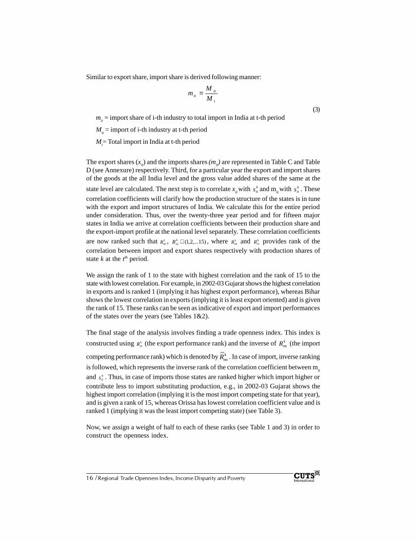
Similar to export share, import share is derived following manner:
t
itit M
Mm =
(3)m
it = import share of i-th industry to total import in India at t-th period
Mit = import of i-th industry at t-th period
Mt= Total import in India at t-th period
The export shares (xit) and the imports shares (mit) are represented in Table C and TableD (see Annexure) respectively. Third, for a particular year the export and import sharesof the goods at the all India level and the gross value added shares of the same at the
state level are calculated. The next step is to correlate xit with k
its and mit with k
its . These
correlation coefficients will clarify how the production structure of the states is in tunewith the export and import structures of India. We calculate this for the entire periodunder consideration. Thus, over the twenty-three year period and for fifteen majorstates in India we arrive at correlation coefficients between their production share andthe export-import profile at the national level separately. These correlation coefficients
are now ranked such that kmtR , )15,...2,1(∈k
xtR , where kmtR and k
xtR provides rank of thecorrelation between import and export shares respectively with production shares ofstate k at the tth period.
We assign the rank of 1 to the state with highest correlation and the rank of 15 to thestate with lowest correlation. For example, in 2002-03 Gujarat shows the highest correlationin exports and is ranked 1 (implying it has highest export performance), whereas Biharshows the lowest correlation in exports (implying it is least export oriented) and is giventhe rank of 15. These ranks can be seen as indicative of export and import performancesof the states over the years (see Tables 1&2).
The final stage of the analysis involves finding a trade openness index. This index is
constructed using kxtR (the export performance rank) and the inverse of kmtR (the import
competing performance rank) which is denoted bykmtR
~. In case of import, inverse ranking
is followed, which represents the inverse rank of the correlation coefficient between mit
and kits . Thus, in case of imports those states are ranked higher which import higher or
contribute less to import substituting production, e.g., in 2002-03 Gujarat shows thehighest import correlation (implying it is the most import competing state for that year),and is given a rank of 15, whereas Orissa has lowest correlation coefficient value and isranked 1 (implying it was the least import competing state) (see Table 3).
Now, we assign a weight of half to each of these ranks (see Table 1 and 3) in order toconstruct the openness index.
Regional Trade O
penness Index, Income D
isparity and Poverty / 17
Table 1: Ranks of Correlation Coefficients between Export Share and GVA Share of Industries in Various States
1980-81 1981-82 1982-83 1983-84 1984-85 1985-86 1986-87 1987-88 1988-89 1989-90 1990-91
Andhra Pradesh 7.5 8 6 4.5 6.5 5.5 4 8 9 9 10
Assam 11.5 12.5 10 11 9 13 14 13 11.5 13 13
Bihar 15 15 15 15 15 15 15 15 15 15 15
Gujarat 1.5 1 1 2 1 1 2 1 2 2 2
Haryana 7.5 4 10 9 6.5 12 12.5 11.5 11.5 12 12
Karnataka 5 8 10 7.5 10 8 6.5 10 8 11 8.5
Kerala 10 10.5 4 3 3 7 10 9 7 7.5 7
Madhya Pradesh 11.5 14 13 12 13 10 5 11.5 13 10 11
Maharashtra 13 10.5 3 1 2 4 11 3 3 3 3
Orissa 14 12.5 14 13 12 11 12.5 14 14 14 14
Punjab 7.5 5.5 5 10 11 5.5 6.5 4 4 4 4.5
Rajasthan 4 3 7 6 5 3 3 5 6 5 4.5
Tamil Nadu 1.5 2 2 4.5 4 2 1 2 1 1 1
Uttar Pradesh 7.5 5.5 8 7.5 8 9 9 7 10 7.5 8.5
West Bengal 3 8 12 14 14 14 8 6 5 6 6
Continue......

18 / Regional Trade O
penness Index, Income D
isparity and Poverty
1991-92 1992-93 1993-94 1994-95 1995-96 1996-97 1997-98 1998-99 1999-00 2000-01 2001-02 2002-03
Andhra Pradesh 12 9 9 12 9.5 12 11 10 11 12 10 10
Assam 13 13 14 14 14 13 13.5 14 14 13.5 15 12
Bihar 15 15 15 15 15 15 15 13 13 13.5 14 15
Gujarat 2 2 2 2 2 3.5 2 2 2 2 1 1
Haryana 11 11.5 11 10.5 12 10 13.5 12 12 10 12.5 14
Karnataka 9 10 6 7 7 8 5 6 8 7.5 4 4
Kerala 10 11.5 12 9 9.5 11 9.5 11 9 9 9 9
Madhya Pradesh 7.5 8 8 8 8 7 4 8 6.5 4 8 6
Maharashtra 3 4 3 3 5 3.5 3 3 4 3 3 3
Orissa 14 14 13 13 13 14 12 15 15 15 12.5 13
Punjab 4 6 5 5 4 3.5 6 5 3 6 6 8
Rajasthan 5 3 4 4 3 3.5 8 4 5 5 5 5
Tamil Nadu 1 1 1 1 1 1 1 1 1 1 2 2
Uttar Pradesh 7.5 7 10 10.5 11 9 9.5 9 10 11 11 11
West Bengal 6 5 7 6 6 6 7 7 6.5 7.5 7 7
Note: The state with highest correlation is assigned rank 1 and vice-versa.

Regional Trade O
penness Index, Income D
isparity and Poverty / 19
Table 2: Ranks of Correlation Coefficients between Import Share and GVA Share Of Industries in Various States
1980-81 1981-82 1982-83 1983-84 1984-85 1985-86 1986-87 1987-88 1988-89 1989-90 1990-91
Andhra Pradesh 7 9.5 9 4 6 6.5 6 11 9 13 12
Assam 15 11 13 14 12.5 9.5 13 15 14 5 4
Bihar 13 9.5 5.5 12 9 14 8 3.5 4 3 2
Gujarat 2 2 1 2 1 1 2 1 1 4 3
Haryana 9 5 5.5 6.5 5 6.5 5 5 10 8.5 11
Karnataka 5.5 8 7 6.5 11 5 4 7 7 8.5 9.5
Kerala 4 3.5 4 5 4 4 9.5 6 5.5 2 5
Madhya Pradesh 8 6.5 12 10.5 7.5 12 7 9 5.5 10 13
Maharashtra 1 1 2 1 2 2 1 2 2 1 1
Orissa 12 15 15 15 15 15 14 13 8 6 9.5
Punjab 5.5 6.5 8 10.5 12.5 9.5 15 14 13 14 15
Rajasthan 14 14 14 13 10 11 11.5 12 15 15 14
Tamil Nadu 3 3.5 3 3 3 3 3 3.5 3 7 6
Uttar Pradesh 10.5 13 11 8.5 7.5 8 11.5 8 11 11 7
West Bengal 10.5 12 10 8.5 14 13 9.5 10 12 12 8
Continue......

20 / Regional Trade O
penness Index, Income D
isparity and Poverty
1991-92 1992-93 1993-94 1994-95 1995-96 1996-97 1997-98 1998-99 1999-00 2000-01 2001-02 2002-03
Andhra Pradesh 9.5 9 10 9 9 11 9 7.5 8.5 8 6 6
Assam 3 4 3 5 5 4 4 10 4 4 7 3
Bihar 5 5 5 4 6.5 7.5 10 12 6 6 10 8
Gujarat 2 1 1 1 1 1 2 2 1 2 1 1
Haryana 11 13 9 15 13 9 8 3 11 8 12 11
Karnataka 8 10 11 7 6.5 5 5 4 10 5 4 5
Kerala 4 3 4 10 4 7.5 3 5 3 3 3 4
Madhya Pradesh 15 12 12 11 10.5 12 11 11 7 10.5 8 7
Maharashtra 1 2 2 2 2 2 1 1 2 1 2 2
Orissa 12 11 13 12 12 10 13 15 15 15 15 15
Punjab 13 15 15 13.5 14 14 15 13.5 12 12 14 14
Rajasthan 14 14 14 13.5 15 15 14 13.5 13 10.5 12 10
Tamil Nadu 6 6 6 3 3 3 7 6 5 13 5 13
Uttar Pradesh 7 8 7 6 8 6 6 7.5 8.5 8 9 9
West Bengal 9.5 7 8 8 10.5 13 12 9 14 14 12 12
Note: The state with highest correlation is assigned rank 1 and vice-versa.

Regional Trade O
penness Index, Income D
isparity and Poverty / 21
Table 3: Inverse Ranks of Correlation Coefficients between Import Share and GVA Share Of Industries in Various States
1980-81 1981-82 1982-83 1983-84 1984-85 1985-86 1986-87 1987-88 1988-89 1989-90 1990-91
Andhra Pradesh 9 6.5 7 12 10 9.5 10 5 7 3 4
Assam 1 5 3 2 3.5 6.5 3 1 2 11 12
Bihar 3 6.5 10.5 4 7 2 8 12.5 12 13 14
Gujarat 14 14 15 14 15 15 14 15 15 12 13
Haryana 7 11 10.5 9.5 11 9.5 11 11 6 7.5 5
Karnataka 10.5 8 9 9.5 5 11 12 9 9 7.5 6.5
Kerala 12 12.5 12 11 12 12 6.5 10 10.5 14 11
Madhya Pradesh 8 9.5 4 5.5 8.5 4 9 7 10.5 6 3
Maharashtra 15 15 14 15 14 14 15 14 14 15 15
Orissa 4 1 1 1 1 1 2 3 8 10 6.5
Punjab 10.5 9.5 8 5.5 3.5 6.5 1 2 3 2 1
Rajasthan 2 2 2 3 6 5 4.5 4 1 1 2
Tamil Nadu 13 12.5 13 13 13 13 13 12.5 13 9 10
Uttar Pradesh 5.5 3 5 7.5 8.5 8 4.5 8 5 5 9
West Bengal 5.5 4 6 7.5 2 3 6.5 6 4 4 8
Continue......

22 / Regional Trade O
penness Index, Income D
isparity and Poverty
1991-92 1992-93 1993-94 1994-95 1995-96 1996-97 1997-98 1998-99 1999-00 2000-01 2001-02 2002-03
Andhra Pradesh 6.5 7 6 7 7 5 7 8.5 7.5 8 10 10
Assam 13 12 13 11 11 12 12 6 12 12 9 13
Bihar 11 11 11 12 9.5 8.5 6 4 10 10 6 8
Gujarat 14 15 15 15 15 15 14 14 15 14 15 15
Haryana 5 3 7 1 3 7 8 13 5 8 4 5
Karnataka 8 6 5 9 9.5 11 11 12 6 11 12 11
Kerala 12 13 12 6 12 8.5 13 11 13 13 13 12
Madhya Pradesh 1 4 4 5 5.5 4 5 5 9 5.5 8 9
Maharashtra 15 14 14 14 14 14 15 15 14 15 14 14
Orissa 4 5 3 4 4 6 3 1 1 1 1 1
Punjab 3 1 1 2.5 2 2 1 2.5 4 4 2 2
Rajasthan 2 2 2 2.5 1 1 2 2.5 3 5.5 4 6
Tamil Nadu 10 10 10 13 13 13 9 10 11 3 11 3
Uttar Pradesh 9 8 9 10 8 10 10 8.5 7.5 8 7 7
West Bengal 6.5 9 8 8 5.5 3 4 7 2 2 4 4
Note: The state with lowest correlation is assigned rank 1 and vice-versa.
Regional Trade Openness Index, Income Disparity and Poverty / 23
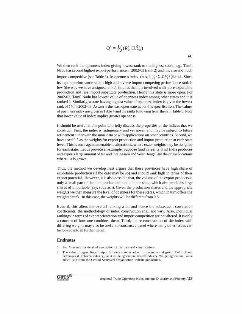
)~
(21 k
mtkxt
kt RRO +=
(4)
We then rank the openness index giving lowest rank to the highest score, e.g., TamilNadu has second highest export performance in 2002-03 (rank 2) and it is also not much
import competitive (see Table 3). Its openness index, thus, is( ) ( ) 5.23*212*2
1 =+ . Since
its export performance rank is high and inverse import competing performance rank islow (the way we have assigned ranks), implies that it is involved with more exportableproduction and less import substitute production. Hence this state is more open. For2002-03, Tamil Nadu has lowest value of openness index among other states and it isranked 1. Similarly, a state having highest value of openness index is given the lowestrank of 15. In 2002-03, Assam is the least open state as per this specification. The valuesof openness index are given in Table 4 and the ranks following from them in Table 5. Notethat lower value of index implies greater openness.
It should be useful at this point to briefly discuss the properties of the indices that weconstruct. First, the index is rudimentary and yet novel, and may be subject to futurerefinement either with the same data or with applications on other countries. Second, wehave used 0.5 as the weights for export production and import production at each statelevel. This is once again amenable to alterations, where exact weights may be assignedfor each state. Let us provide an example. Suppose (and in reality, it is) India producesand exports large amount of tea and that Assam and West Bengal are the prime locationswhere tea is grown.
Thus, the method we develop next argues that these provinces have high share ofexportable production (if the case may be so) and should rank high in terms of theirexport potential. However, it is also possible that, the volume of the export products isonly a small part of the total production bundle in the state, which also produces largeshares of importable (say, soda ash). Given the production shares and the appropriateweights we then measure the level of openness for these states, which in turn offers theweighted rank. In this case, the weights will be different from 0.5.
Even if, this alters the overall ranking a bit and hence the subsequent correlationcoefficients, the methodology of index construction shall not vary. Also, individualrankings in terms of export orientation and import competition are not altered. It is onlya concern of how one combines them. Third, the re-construction of the index withdiffering weights may also be useful to construct a panel where many other issues canbe looked into in further detail.
Endnotes1 See Annexure for detailed description of the data and classifications.
2 The value of agricultural output for each state is added to the industrial group 15-16 (Food,Beverages & Tobacco industry), as it is the agriculture related industry. We get agricultural valueadded data from the Central Statistical Organisation website/publication.

24 / Regional Trade O
penness Index, Income D
isparity and Poverty
Table 4: Yearly Openness Index Values of Indian States
1980-81 1981-82 1982-83 1983-84 1984-85 1985-86 1986-87 1987-88 1988-89 1989-90 1990-91
Andhra Pradesh 8.25 7.25 6.5 8.25 8.25 7.5 7 6.5 8 6 7
Assam 6.25 8.75 6.5 6.5 6.25 9.75 8.5 7 6.75 12 12.5
Bihar 9 10.75 12.75 9.5 11 8.5 11.5 13.75 13.5 14 14.5
Gujarat 7.75 7.5 8 8 8 8 8 8 8.5 7 7.5
Haryana 7.25 7.5 10.25 9.25 8.75 10.75 11.75 11.25 8.75 9.75 8.5
Karnataka 7.75 8 9.5 8.5 7.5 9.5 9.25 9.5 8.5 9.25 7.5
Kerala 11 11.5 8 7 7.5 9.5 8.25 9.5 8.75 10.75 9
Madhya Pradesh 9.75 11.75 8.5 8.75 10.75 7 7 9.25 11.75 8 7
Maharashtra 14 12.75 8.5 8 8 9 13 8.5 8.5 9 9
Orissa 9 6.75 7.5 7 6.5 6 7.25 8.5 11 12 10.25
Punjab 9 7.5 6.5 7.75 7.25 6 3.75 3 3.5 3 2.75
Rajasthan 3 2.5 4.5 4.5 5.5 4 3.75 4.5 3.5 3 3.25
Tamil Nadu 7.25 7.25 7.5 8.75 8.5 7.5 7 7.25 7 5 5.5
Uttar Pradesh 6.5 4.25 6.5 7.5 8.25 8.5 6.75 7.5 7.5 6.25 8.75
West Bengal 4.25 6 9 10.75 8 8.5 7.25 6 4.5 5 7
Continue......
Regional Trade O
penness Index, Income D
isparity and Poverty / 25
1991-92 1992-93 1993-94 1994-95 1995-96 1996-97 1997-98 1998-99 1999-00 2000-01 2001-02 2002-03
Andhra Pradesh 9.25 8 7.5 9.5 8.25 8.5 9 9.25 9.25 10 10 10
Assam 13 12.5 13.5 12.5 12.5 12.5 12.75 10 13 12.75 12 12.5
Bihar 13 13 13 13.5 12.25 11.75 10.5 8.5 11.5 11.75 10 11.5
Gujarat 8 8.5 8.5 8.5 8.5 9.25 8 8 8.5 8 8 8
Haryana 8 7.25 9 5.75 7.5 8.5 10.75 12.5 8.5 9 8.25 9.5
Karnataka 8.5 8 5.5 8 8.25 9.5 8 9 7 9.25 8 7.5
Kerala 11 12.25 12 7.5 10.75 9.75 11.25 11 11 11 11 10.5
Madhya Pradesh 4.25 6 6 6.5 6.75 5.5 4.5 6.5 7.75 4.75 8 7.5
Maharashtra 9 9 8.5 8.5 9.5 8.75 9 9 9 9 8.5 8.5
Orissa 9 9.5 8 8.5 8.5 10 7.5 8 8 8 6.75 7
Punjab 3.5 3.5 3 3.75 3 2.75 3.5 3.75 3.5 5 4 5
Rajasthan 3.5 2.5 3 3.25 2 2.25 5 3.25 4 5.25 4.5 5.5
Tamil Nadu 5.5 5.5 5.5 7 7 7 5 5.5 6 2 6.5 2.5
Uttar Pradesh 8.25 7.5 9.5 10.25 9.5 9.5 9.75 8.75 8.75 9.5 9 9
West Bengal 6.25 7 7.5 7 5.75 4.5 5.5 7 4.25 4.75 5.5 5.5

26 / Regional Trade O
penness Index, Income D
isparity and Poverty
Table 5: Yearly Openness Index Ranks of Indian States
1980-81 1981-82 1982-83 1983-84 1984-85 1985-86 1986-87 1987-88 1988-89 1989-90 1990-91
Andhra Pradesh 9 5.5 3.5 9 10.5 5.5 5 4 7 5 5
Assam 3 11 3.5 2 2 14 11 5 4 13.5 14
Bihar 11 12 15 14 15 9 13 15 15 15 15
Gujarat 7.5 8 8.5 7.5 8 7 9 8 9 7 7.5
Haryana 5.5 8 14 13 13 15 14 14 11.5 11 9
Karnataka 7.5 10 13 10 5.5 12.5 12 12.5 9 10 7.5
Kerala 14 13 8.5 3.5 5.5 12.5 10 12.5 11.5 12 11.5
Madhya Pradesh 13 14 10.5 11.5 14 4 5 11 14 8 5
Maharashtra 15 15 10.5 7.5 8 11 15 9.5 9 9 11.5
Orissa 11 4 6.5 3.5 3 2.5 7.5 9.5 13 13.5 13
Punjab 11 8 3.5 6 4 2.5 1.5 1 1.5 1.5 1
Rajasthan 1 1 1 1 1 1 1.5 2 1.5 1.5 2
Tamil Nadu 5.5 5.5 6.5 11.5 12 5.5 5 6 5 3.5 3
Uttar Pradesh 4 2 3.5 5 10.5 9 3 7 6 6 10
West Bengal 2 3 12 15 8 9 7.5 3 3 3.5 5
Continue......
Regional Trade O
penness Index, Income D
isparity and Poverty / 27
1991-92 1992-93 1993-94 1994-95 1995-96 1996-97 1997-98 1998-99 1999-00 2000-01 2001-02 2002-03
Andhra Pradesh 12 8.5 6.5 12 7.5 6.5 9.5 12 12 12 12.5 12
Assam 14.5 14 15 14 15 15 15 13 15 15 15 15
Bihar 14.5 15 14 15 14 14 12 8 14 14 12.5 14
Gujarat 6.5 10 9.5 10 9.5 9 7.5 6.5 8.5 6.5 7 8
Haryana 6.5 6 11 3 6 6.5 13 15 8.5 8.5 9 11
Karnataka 9 8.5 3.5 8 7.5 10.5 7.5 10.5 5 10 7 6.5
Kerala 13 13 13 7 13 12 14 14 13 13 14 13
Madhya Pradesh 3 4 5 4 4 4 2 4 6 2.5 7 6.5
Maharashtra 10.5 11 9.5 10 11.5 8 9.5 10.5 11 8.5 10 9
Orissa 10.5 12 8 10 9.5 13 6 6.5 7 6.5 5 5
Punjab 1.5 2 1.5 2 2 2 1 2 1 4 1 2
Rajasthan 1.5 1 1.5 1 1 1 3.5 1 2 5 2 3.5
Tamil Nadu 4 3 3.5 5.5 5 5 3.5 3 4 1 4 1
Uttar Pradesh 8 7 12 13 11.5 10.5 11 9 10 11 11 10
West Bengal 5 5 6.5 5.5 3 3 5 5 3 2.5 3 3.5
Note: The state with lowest openness index value is assigned rank 1 and vice-versa.

28 / Regional Trade Openness Index, Income Disparity and Poverty
5Relationship between Openness and
Inter-regional Income Disparity
Attempts have been made in this section to relate the openness at the state level withtheir income pattern over time and it is worked out in three different ways. Before
doing that, however, we observe the income disparity among the 15 major states overtime in terms of the coefficients of variation in PCNSDP. If one looks into the incomevariation among the major states in India, it reveals an increasing trend over time asbetween 1980 and 2003. Figure 1 shows that the coefficient of variation (standarddeviation divided by mean) in income among major states has increased from 31.09percent in 1980-81 to 38.16 percent in 2002-03. In other words, regional disparity hasincreased by about 25 percent during the given period. This encourages us to examineif there is any relationship between interregional income disparity and trade opennessfor the Indian states between 1980-81 and 2002-03.
Figure 1: Trend of Coefficient of Variation of PCNSDP acrossMajor States in India, 1980-81 to 2002-03
0
5
10
15
20
25
30
35
40
45
1980
-81
1981
-82
1982
-83
1983
-84
1984
-85
1985
-86
1986
-87
1987
-88
1988
-89
1989
-90
1990
-91
1991
-92
1992
-93
1993
-94
1994
-95
1995
-96
1996
-97
1997
-98
1998
-99
1999
-00
2000
-01
2001
-02
2002
-03
Year
CV
(%
)
CV

Regional Trade Openness Index, Income Disparity and Poverty / 29
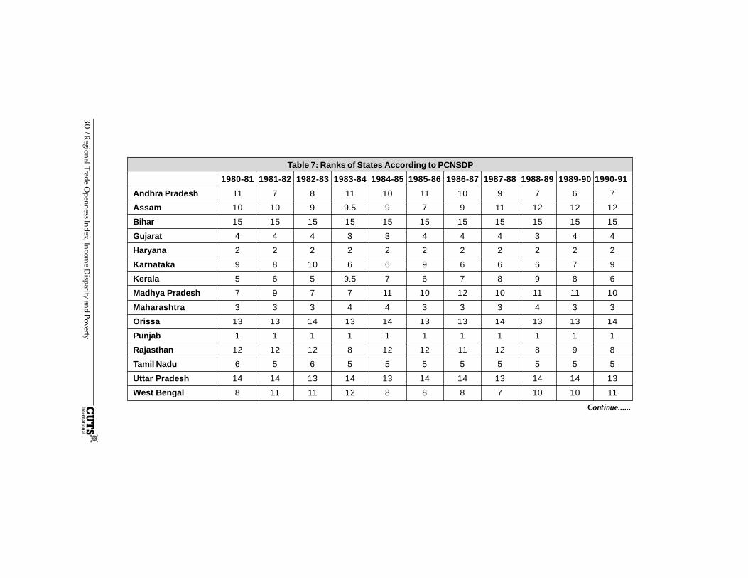
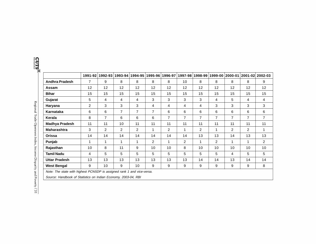
5.1 Relation between Openness and PCNSDP of the StatesAt first, the states are ranked according to their PCNSDP such that. We get the data onPCNSDP of these states from the Central Statistical Organisation (CSO). However, thisdata is divided into two series. The old series is based in 1980-81 prices, whereas, thenew series is based on 1993-94 prices. To make the two series compatible the old serieshave been converted to 1993-94 prices and subsequently, we ranked the states accordingto their PCNSDP from 1980-81 to 2002-03. We rank states having higher PCNSDP withhigher ranks, for e.g., in 2002-03 Maharashtra has the highest PCNSDP (Rs. 15,466)among the 15 states. So, it is ranked at 1. For the same year, Bihar has lowest PCNSDP(Rs. 4,448) and is given the rank of 15. These ranks for all the years are shown inTable 6.
Table 6: Coefficient of Variation of PCNSDP across Major States in India
Year Coefficient of variation of PCNSDP
1980-81 31.09
1981-82 31.45
1982-83 32.44
1983-84 30.66
1984-85 32.28
1985-86 34.64
1986-87 34.72
1987-88 35.05
1988-89 34.43
1989-90 36.03
1990-91 35.99
1991-92 36.37
1992-93 38.65
1993-94 35.81
1994-95 35.37
1995-96 36.82
1996-97 37.32
1997-98 36.88
1998-99 37.15
1999-00 37.07
2000-01 36.66
2001-02 36.36
2002-03 38.16
Source: Handbook of Statistics on Indian Economy, 2003-04, RBI
30 / Regional Trade O
penness Index, Income D
isparity and Poverty
Table 7: Ranks of States According to PCNSDP
1980-81 1981-82 1982-83 1983-84 1984-85 1985-86 1986-87 1987-88 1988-89 1989-90 1990-91
Andhra Pradesh 11 7 8 11 10 11 10 9 7 6 7
Assam 10 10 9 9.5 9 7 9 11 12 12 12
Bihar 15 15 15 15 15 15 15 15 15 15 15
Gujarat 4 4 4 3 3 4 4 4 3 4 4
Haryana 2 2 2 2 2 2 2 2 2 2 2
Karnataka 9 8 10 6 6 9 6 6 6 7 9
Kerala 5 6 5 9.5 7 6 7 8 9 8 6
Madhya Pradesh 7 9 7 7 11 10 12 10 11 11 10
Maharashtra 3 3 3 4 4 3 3 3 4 3 3
Orissa 13 13 14 13 14 13 13 14 13 13 14
Punjab 1 1 1 1 1 1 1 1 1 1 1
Rajasthan 12 12 12 8 12 12 11 12 8 9 8
Tamil Nadu 6 5 6 5 5 5 5 5 5 5 5
Uttar Pradesh 14 14 13 14 13 14 14 13 14 14 13
West Bengal 8 11 11 12 8 8 8 7 10 10 11
Continue......
Regional Trade O
penness Index, Income D
isparity and Poverty / 31
1991-92 1992-93 1993-94 1994-95 1995-96 1996-97 1997-98 1998-99 1999-00 2000-01 2001-02 2002-03
Andhra Pradesh 7 9 8 8 8 8 10 8 8 8 8 9
Assam 12 12 12 12 12 12 12 12 12 12 12 12
Bihar 15 15 15 15 15 15 15 15 15 15 15 15
Gujarat 5 4 4 4 3 3 3 3 4 5 4 4
Haryana 2 3 3 3 4 4 4 4 3 3 3 3
Karnataka 6 6 7 7 7 6 6 6 6 6 6 6
Kerala 8 7 6 6 6 7 7 7 7 7 7 7
Madhya Pradesh 11 11 10 11 11 11 11 11 11 11 11 11
Maharashtra 3 2 2 2 1 2 1 2 1 2 2 1
Orissa 14 14 14 14 14 14 14 13 13 14 13 13
Punjab 1 1 1 1 2 1 2 1 2 1 1 2
Rajasthan 10 8 11 9 10 10 8 10 10 10 10 10
Tamil Nadu 4 5 5 5 5 5 5 5 5 4 5 5
Uttar Pradesh 13 13 13 13 13 13 13 14 14 13 14 14
West Bengal 9 10 9 10 9 9 9 9 9 9 9 8
Note: The state with highest PCNSDP is assigned rank 1 and vice-versa.
Source: Handbook of Statistics on Indian Economy, 2003-04, RBI

32 / Regional Trade Openness Index, Income Disparity and Poverty
These two sets of ranks (see in Table 1 and 3) are ultimately correlated and the presentedin a scatter-plot in Figure 2 to find out the dynamics of export-led regional development.This figure clearly shows that the trend for the correlation coefficients is increasing overtime, which directly implies that the interregional disparity as explained by exportperformance of the states is on the rise. We also find that the values of the correlationcoefficients are higher after the reform period than before it.
Figure 2: Correlation Coefficients and Trend Line between Export Performance andPCNSDP Ranks across States (1980-81 to 2002-03)
R2 = 0.3676
0
0.1
0.2
0.3
0.4
0.5
0.6
0.7
0.8
1980
-81
1981
-82
1982
-83
1983
-84
1984
-85
1985
-86
1986
-87
1987
-88
1988
-89
1989
-90
1990
-91
1991
-92
1992
-93
1993
-94
1994
-95
1995
-96
1996
-97
1997
-98
1998
-99
1999
-200
0
2000
-01
2001
-02
2002
-03
Year
Figure 3: Correlation Coefficients and Trend Line between Import CompetingPerformance and PCNSDP Ranks across States (1980-81 to 2002-03)
R2 = 0.2314
-0.4
-0.2
0
0.2
0.4
0.6
0.8
1
1980-81
1981-82
1982-83
1983-84
1984-85
1985-86
1986-87
1987-88
1988-89
1989-90
1990-91
1991-92
1992-93
1993-94
1994-95
1995-96
1996-97
1997-98
1998-99
1999-20
00
2000-01
2001-02
2002-03
Year

Regional Trade Openness Index, Income Disparity and Poverty / 33
kmtR and k
tR are correlated and the correlation coefficients are presented in the scatter plotin Figure 3. We find that the correlations are positive and the linear trend attached to itis downward sloping, i.e., with time the correlations are becoming weaker. StudyingFigures 2 and 3 it can be said that more export oriented and less import competing statesgain in terms of Income over time.
At last to link states’ openness to trade with their PCNSDP we correlate ktO with k
tR . Thefinal correlation coefficients are plotted in a scatter diagram (see Figure 4). Figure 4 alsoshows that the linear trend attached to the final correlation coefficients is upward rising.This implies that with time the extent of regional income has found gradually strongpositive relationship with the trade openness of that region.
Figure 4: Correlation Coefficients and Trend Line between OpennessIndex and PCNSDP Ranks across States (1980-81 to 2002-03)
R2 = 0.4462
-0.4
-0.3
-0.2
-0.1
0
0.1
0.2
0.3
0.4
0.5
0.6
1980
-81
1982
-83
1984
-85
1986
-87
1988
-89
1990
-91
1992
-93
1994
-95
1996
-97
1998
-99
2000
-01
2002
-03
Year
5.2 Relation between Openness and Dispersion of PCNSDPIn order to examine the nexus between trade openness and regional disparity in anotherway, first we look at the dispersion of income calculating trend of coefficient of variationacross states and try to correlate dispersion of the state with its openness. We have
derived indices of ‘regional disparity’, viz. relative mean deviation in PCNSDP (ktσ ), to
find out relative position of k-th state with respect to mean income at t-th period. Higher
the value of relative mean deviation in PCNSDP (ktσ with sign), the state should be
considered richer on average. It should be noted that sign of ktσ will take positive of
k-th state if PCNSDP is higher than the mean otherwise negative. Then we have ranked
each state on the basis of the principle: ‘state with highest value for ktσ receives rank 1
and vice versa’ and it is reported in Table 7.,

34 / Regional Trade Openness Index, Income Disparity and Poverty
( )
x
xxktk
t
100*−=σ , 032002,..,811980,15,..,1 −−== tk (5)
=ktx PCNSDP for kth state in tth period.
=x Mean of the PCNSDP among states in a give period
Correlation coefficient between rank of states based on ktσ and rank of states based on
openness Index is calculated (ctR ) and presented in Fig. 5. The figure shows a positive
relationship between the rank of states based on stσ and the rank of states based onopenness index. This suggests that a state, which is being more ‘open’, is also becomingmore ‘wealthy’ compared to the other states.
Figure 5: Correlation Coefficient between Openness Index Rank & Rank ofRelative Mean Deviation based on PCNSDP (1980-82 to 2002-03)
R2 = 0.3964
-0.400-0.300-0.200-0.1000.0000.1000.2000.3000.4000.5000.6000.700
1980-81
1982-83
1984-85
1986-87
1988-89
1990-91
1992-93
1994-95
1996-97
1998-99
2000-01
2002-03
Year
corr
elat
ion
coef
ficie
nt
5.3 Relation between Openness and PCNSDP Growth of the States
The growth rate of PCNSDP ( )ktγ is defined by the percentage change of PCNSDP with
respect to pervious year.
( )
kt
kt
ktk
tx
xx
1
1 100*
−
−−=γ , 032002,..,811980,15,...,1 −−== tk (6)
=ktx PCNSDP for kth state in tth period.

Regional Trade Openness Index, Income Disparity and Poverty / 35
We have calculated the value of ktγ for each state, for each year and then ranked each
state on the basis of ktγ using the same principle (see Table 8). As the definition suggests,ktγ can be considered as a measure of wealthy state compared to the other states in tth
period. Correlation coefficient between rank of states based on ktγ and rank of state
Openness Index is also calculated (see Figure 6). The same conclusion can be drawnfrom Figure 6, which portrays a positive relationship, although trend of this correlationdo not show sharp rising trend.
Therefore, all three measures of inter-regional income disparity of states are found to begradually more correlated with the openness of the states over the years. We would liketo emphasise on the fact that this analysis focuses only on the connection betweenexportable/importable production and PCNSDP ranks, ranks of relative mean deviationand ranks of growth of states while controlling for policy changes like trade promotionschemes, foreign exchange regime changes etc., which are introduced ever since thereform period. This might have influenced trade performance and PCNSDP (see Table 9).Nevertheless, the analysis provides ample support in favour of the initial hypothesisthat increases in regional disparity in Indian states has some correlation with their tradeopenness over the years.
Figure 6: Correlation Coefficient between Rank of PCNSDP Growth &Rank of Openness Index (1981-82 to 2002-03)
R2 = 0.025
-0.600
-0.400
-0.200
0.000
0.200
0.400
0.600
0.800
1981
-82
1983
-84
1985
-86
1987
-88
1989
-90
1991
-92
1993
-94
1995
-96
1997
-98
1999
-00
2001
-02
Year
corr
elat
ion
coef
ficie
nt
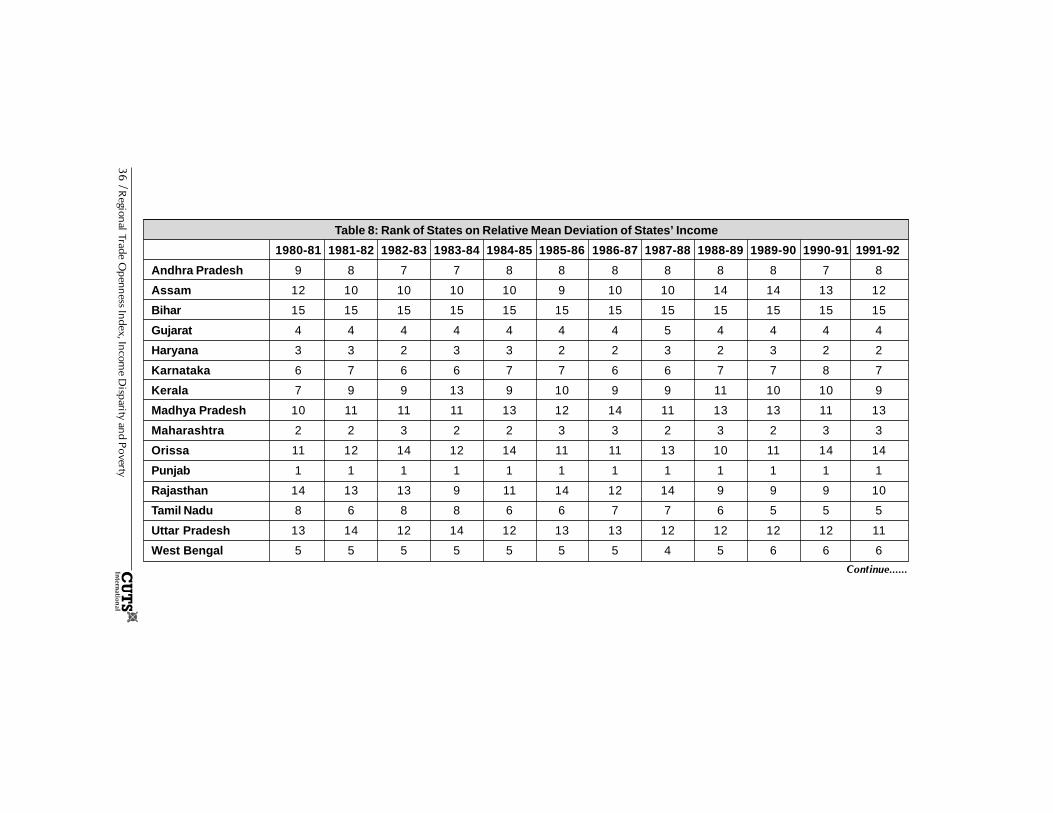
36 / Regional Trade O
penness Index, Income D
isparity and Poverty
Table 8: Rank of States on Relative Mean Deviation of States’ Income
1980-81 1981-82 1982-83 1983-84 1984-85 1985-86 1986-87 1987-88 1988-89 1989-90 1990-91 1991-92
Andhra Pradesh 9 8 7 7 8 8 8 8 8 8 7 8
Assam 12 10 10 10 10 9 10 10 14 14 13 12
Bihar 15 15 15 15 15 15 15 15 15 15 15 15
Gujarat 4 4 4 4 4 4 4 5 4 4 4 4
Haryana 3 3 2 3 3 2 2 3 2 3 2 2
Karnataka 6 7 6 6 7 7 6 6 7 7 8 7
Kerala 7 9 9 13 9 10 9 9 11 10 10 9
Madhya Pradesh 10 11 11 11 13 12 14 11 13 13 11 13
Maharashtra 2 2 3 2 2 3 3 2 3 2 3 3
Orissa 11 12 14 12 14 11 11 13 10 11 14 14
Punjab 1 1 1 1 1 1 1 1 1 1 1 1
Rajasthan 14 13 13 9 11 14 12 14 9 9 9 10
Tamil Nadu 8 6 8 8 6 6 7 7 6 5 5 5
Uttar Pradesh 13 14 12 14 12 13 13 12 12 12 12 11
West Bengal 5 5 5 5 5 5 5 4 5 6 6 6
Continue......

Regional Trade O
penness Index, Income D
isparity and Poverty / 37
1992-93 1993-94 1994-95 1995-96 1996-97 1997-98 1998-99 1999-00 2000-01 2001-02 2002-03
Andhra Pradesh 8 8 8 8 8 10 8 8 8 8 9
Assam 13 12 12 12 12 12 12 12 12 12 12
Bihar 15 15 15 15 15 15 15 15 15 15 15
Gujarat 4 4 4 3 3 3 3 4 5 4 4
Haryana 3 3 3 4 4 4 4 3 3 3 3
Karnataka 7 7 7 7 6 6 6 6 6 6 6
Kerala 10 6 6 6 7 7 7 7 7 7 7
Madhya Pradesh 11 10 11 11 11 11 11 11 11 11 11
Maharashtra 2 2 2 1 2 1 2 1 2 2 1
Orissa 14 14 14 14 14 14 13 13 14 13 13
Punjab 1 1 1 2 1 2 1 2 1 1 2
Rajasthan 9 11 9 10 10 8 10 10 10 10 10
Tamil Nadu 5 5 5 5 5 5 5 5 4 5 5
Uttar Pradesh 12 13 13 13 13 13 14 14 13 14 14
West Bengal 6 9 10 9 9 9 9 9 9 9 8
Note: The state with highest value of relative mean deviation is assigned rank 1 and vice-versa.
Source: Handbook of Statistics on Indian Economy, 2003-04, RBI

38 / Regional Trade Openness Index, Income Disparity and Poverty
Table 9: Rank of States on Growth Rate of PCNSDP
1981-82 1982-831983-84 1984-85 1985-86 1986-87 1987-88 1988-89 1989-90 1990-91 1991-92
Andhra 1 10 10 12 6 13 1 5 3 9 5Pradesh
Assam 3 4 9 10 5 14 9 15 5 10 7
Bihar 8 12 5 2 11 3 13 8 14 4 12
Gujarat 5 13 3 11 14 5 15 2 13 12 15
Haryana 10 3 13 7 1 10 11 3 12 3 10
Karnataka 7 9 6 5 15 1 4 11 7 13 2
Kerala 14 7 15 6 7 12 10 9 2 6 9
Madhya 11 5 8 14 3 15 2 12 11 2 13Pradesh
Maharashtra 9 2 14 4 12 4 3 6 8 14 1
Orissa 13 15 2 13 2 9 12 4 6 15 3
Punjab 4 8 12 3 4 8 6 13 1 11 6
Rajasthan 6 11 1 15 13 2 14 1 15 1 14
Tamil Nadu 2 14 7 1 8 11 5 10 4 5 8
Uttar 12 1 11 9 10 6 8 7 10 7 11Pradesh
West Bengal 15 6 4 8 9 7 7 14 9 8 4
1992-93 1993-941994-95 1995-96 1996-97 1997-98 1998-99 1999-00 2000-01 2001-02 2002-03
Andhra 14 1 9 2 7 14 2 10 3 7 10Pradesh
Assam 11 10 14 13 14 10 15 12 9 10 6
Bihar 15 12 4 15 1 15 9 11 1 15 1
Gujarat 1 14 1 11 2 11 5 14 14 3 2
Haryana 12 9 8 14 3 12 11 6 6 8 5
Karnataka 9 4 10 4 6 5 1 8 2 14 7
Kerala 4 2 6 6 13 8 4 2 7 11 3
Madhya 5 3 15 3 10 6 7 1 15 1 13Pradesh
Maharashtra 3 13 5 8 11 7 3 15 8 6 15
Orissa 13 7 11 5 15 1 13 5 12 2 12
Punjab 7 8 13 9 8 9 8 9 10 12 9
Rajasthan 2 15 2 10 4 2 12 13 13 5 14
Tamil Nadu 6 5 3 7 12 3 10 4 4 13 8
Uttar 10 11 12 12 5 13 14 7 11 9 11Pradesh
West Bengal 8 6 7 1 9 4 6 3 5 4 4
Note: The state with highest growth rate is assigned rank 1 and vice-versa.
Source: Handbook of Statistics on Indian Economy, 2003-04

Regional Trade Openness Index, Income Disparity and Poverty / 39
6Openness Index and Industrial Jobs
As discussed above, the openness at the state level is responsible for substantialdivergence of net state domestic product in India. It is clearly established that the
states with traditional emphasis on production of commodities that are intrinsicallyimport competing in nature have suffered an income loss over these years. On the otherhand, provinces that retained larger share of production in the export category facedimprovement in their PCNSDP. It is, however, not clear from the above results whetherindustrial employment or unemployment is affected by the openness in trade.
Theoretically, it is expected that as trade barriers crumble, i.e. the economy becomesmore open to imports from the rest of the world the import-competing industries mustsuffer. Output and employment in these industries are expected to contract. On the otherhand, an increase in exports, or at least the potential of it, must imply higher output andemployment in those industries, which are either direct producers of export commoditiesor are somehow linked to it as, viz. suppliers of intermediate commodities.
This particular section takes up this exercise where we link trade openness to annualgrowth in employees and annual growth in workers across various industries in India asclassified by the SIC. The results given in Tables 10 and 11 display that across industrytypes (SIC 20-21 to SIC 37) the correlation coefficient between regional openness indexand growth of workers (blue-collared jobs in the factories earning ‘wages’, as categorizedby the Annual Survey of Industries) and that of employees (white-collared jobs inrespective industry types, earning ‘salaries’, ASI) fluctuates around the zero value andsome of these are statistically significant. The procedure is as follows: first we calculatethe state specific growth rate of employees and workers for each industry type between1981-82 and 1997-98.
Second, we find the correlation of such growth rates (over these years) with that of tradeopenness across states and come up with a value. So, in Table 10 for example, thecorrelation coefficient between TOI and growth of employees across states for theindustry type 20-21 and for the year 1981-82 is (–0.041). All other values are similarlycalculated and reported in Tables 10 and 11 (also see figures 7 and 8).

40 / Regional Trade O
penness Index, Income D
isparity and Poverty
Table 10: Correlation between Growth of Workers and TOI across Industries
Years SIC20-21 SIC22 SIC23 SIC25 SIC26 SIC27 SIC28 SIC29 SIC30 SIC33 SIC35-36 SIC37
1981-82 -0.062 0.286 -0.094 -0.039 -0.153 -0.103 0.069 -0.085 -0.199 -0.097 0.083 -0.265
1982-83 0.111 -0.381 0.254 0.114 0.399 0.238 -0.228 0.216 -0.222 0.254 0.273 0.357
1983-84 -0.263 0.066 -0.14 -0.221 -0.26 -0.122 -0.205 -0.507 -0.276 -0.137 -0.46 0.13
1984-85 -0.462 -0.054 0.019 -0.047 0.217 -0.059 0.132 -0.109 0.338 0.301 -0.027 -0.388
1985-86 0.314 0.103 -0.447 0.254 -0.721 0.198 0.195 0.019 -0.636 0.022 -0.217 0.224
1986-87 -0.076 -0.491 0.189 0.258 0.06 -0.439 0.013 0.107 -0.278 0.071 -0.026 0.065
1987-88 -0.38 0.737 -0.231 -0.15 -0.365 0.409 -0.085 -0.128 0.054 -0.305 0.449 0.065
1988-89 -0.1 -0.446 0.457 0.539 0.309 0.143 -0.111 -0.359 0.088 0.47 -0.319 0.121
1989-90 0.186 0.191 -0.479 -0.364 -0.298 -0.205 -0.293 0.22 0.032 -0.246 -0.434 -0.35
1990-91 0.363 0.276 -0.294 -0.227 0.522 -0.075 0.421 -0.113 -0.327 -0.099 -0.151 0.023
1991-92 -0.194 -0.62 0.442 0.002 0.157 -0.211 0.543 -0.536 0.365 0.318 0.028 -0.214
1992-93 0.243 -0.035 -0.069 -0.132 -0.151 -0.062 -0.024 -0.004 0.347 -0.241 -0.568 0.393
1993-94 -0.434 0.446 -0.426 -0.277 -0.07 -0.07 0.066 -0.097 -0.313 -0.406 -0.259 -0.254
1994-95 0.191 -0.432 -0.307 0.37 0.354 -0.218 -0.077 0.026 0.293 0 0.318 0.436
1995-96 -0.132 -0.137 0.428 0.026 -0.697 -0.169 0.152 -0.033 0.072 0.221 0.068 0.026
1996-97 -0.128 -0.033 -0.528 0.272 -0.242 -0.568 -0.149 -0.386 -0.526 0.066 -0.186 0.02
1997-98 -0.261 -0.101 -0.16 -0.527 0.417 0.337 0.284 0.186 0.275 0.125 -0.343 0.143

Regional Trade O
penness Index, Income D
isparity and Poverty / 41
Table 11: Correlation between TOI and Growth of Employees across Industries (SIC)
Years SIC20-21 SIC22 SIC23 SIC25 SIC26 SIC27 SIC28 SIC29 SIC30 SIC33 SIC35-36 SIC37
1981-82 -0.041 0.357 0.464 -0.022 -0.169 -0.46 0.012 -0.114 -0.319 -0.445 0.032 -0.243
1982-83 0.007 -0.329 0.294 0.134 0.401 0.347 -0.157 0.265 -0.206 0.285 0.255 0.345
1983-84 0.001 0.041 -0.086 -0.199 -0.279 -0.329 -0.09 -0.505 -0.281 -0.301 -0.557 0.155
1984-85 -0.505 -0.045 -0.022 -0.108 0.167 -0.03 0.143 -0.057 0.345 0.489 -0.444 -0.391
1985-86 0.151 0.157 -0.451 0.272 -0.706 0.21 0.247 -0.064 -0.631 -0.055 -0.233 0.236
1986-87 -0.035 -0.49 0.251 0.243 0.06 -0.461 -0.034 0.035 -0.355 -0.08 0.093 0.04
1987-88 -0.344 0.706 -0.341 -0.134 -0.363 0.425 -0.089 -0.145 0.051 -0.259 0.283 0.051
1988-89 -0.012 -0.494 0.468 0.533 0.35 0.173 -0.111 -0.362 0.154 0.468 -0.228 0.149
1989-90 0.218 0.238 -0.469 -0.365 -0.279 -0.224 -0.3 0.257 -0.027 -0.219 -0.519 -0.378
1990-91 0.371 0.212 -0.293 -0.195 0.53 -0.101 0.403 -0.088 -0.386 -0.101 -0.057 -0.005
1991-92 -0.197 -0.636 0.456 0.001 0.035 -0.153 0.59 -0.551 0.278 0.274 -0.011 -0.259
1992-93 0.222 -0.079 -0.145 -0.25 -0.043 -0.172 0 -0.004 0.343 -0.055 -0.521 0.389
1993-94 -0.377 0.458 -0.398 -0.233 -0.162 0.128 0.029 -0.046 -0.295 -0.098 -0.259 -0.218
1994-95 0.262 -0.44 -0.324 0.369 0.352 -0.305 -0.043 -0.009 0.301 0.03 0.319 0.441
1995-96 -0.142 -0.193 0.428 0.021 -0.664 -0.212 0.178 0.07 0.114 0.184 0.183 -0.027
1996-97 -0.196 -0.065 -0.629 0.281 -0.149 -0.564 -0.235 -0.441 -0.362 0.111 0.011 -0.028
1997-98 -0.254 -0.07 -0.109 -0.191 0.055 0.375 0.147 0.077 0.074 0.041 -0.295 0.205

42 / Regional Trade Openness Index, Income Disparity and Poverty
-0.8
-0.6
-0.4
-0.2
0
0.2
0.4
0.6
0.8
1
1981-82
1982-83
1983-84
1984-85
1985-86
1986-87
1987-88
1988-89
1989-90
1990-91
1991-92
1992-93
1993-94
1994-95
1995-96
1996-97
1997-98
Years
Cor
rela
tion
Coe
ffici
ent
SIC20-21 SIC22 SIC23 SIC25 SIC26 SIC27
SIC28 SIC29 SIC30 SIC33 SIC35-36 SIC37
( )
-0.8
-0.6
-0.4
-0.2
0
0.2
0.4
0.6
0.8
1981-82
1982-83
1983-84
1984-85
1985-86
1986-87
1987-88
1988-89
1989-90
1990-91
1991-92
1992-93
1993-94
1994-95
1995-96
1996-97
1997-98
Years
Cor
rela
tion
Coe
ffici
ent
SIC20-21 SIC22 SIC23 SIC25 SIC26 SIC27
SIC28 SIC29 SIC30 SIC33 SIC35-36 SIC37
Figure 8: Correlation between TOI and Growth ofEmployees across Industries (SIC)
Figure 7: Correlation between Regional TOI and Growth ofWorkers across Industries (SIC)
Clearly, the correlation coefficients show that there is no uniform and monotonic relationbetween the growth rates of employees and workers and the TOI. However, fittingsecond-order polynomials to the evolving patterns in the correlation coefficient revealsthat in most cases the relationship inverted U-shaped (or at best concave), in that, it isincreasing till the immediate pre-reform period after which it falls at an increasing rate. Inother words, the trade openness (or lack of it) may have significantly affected the
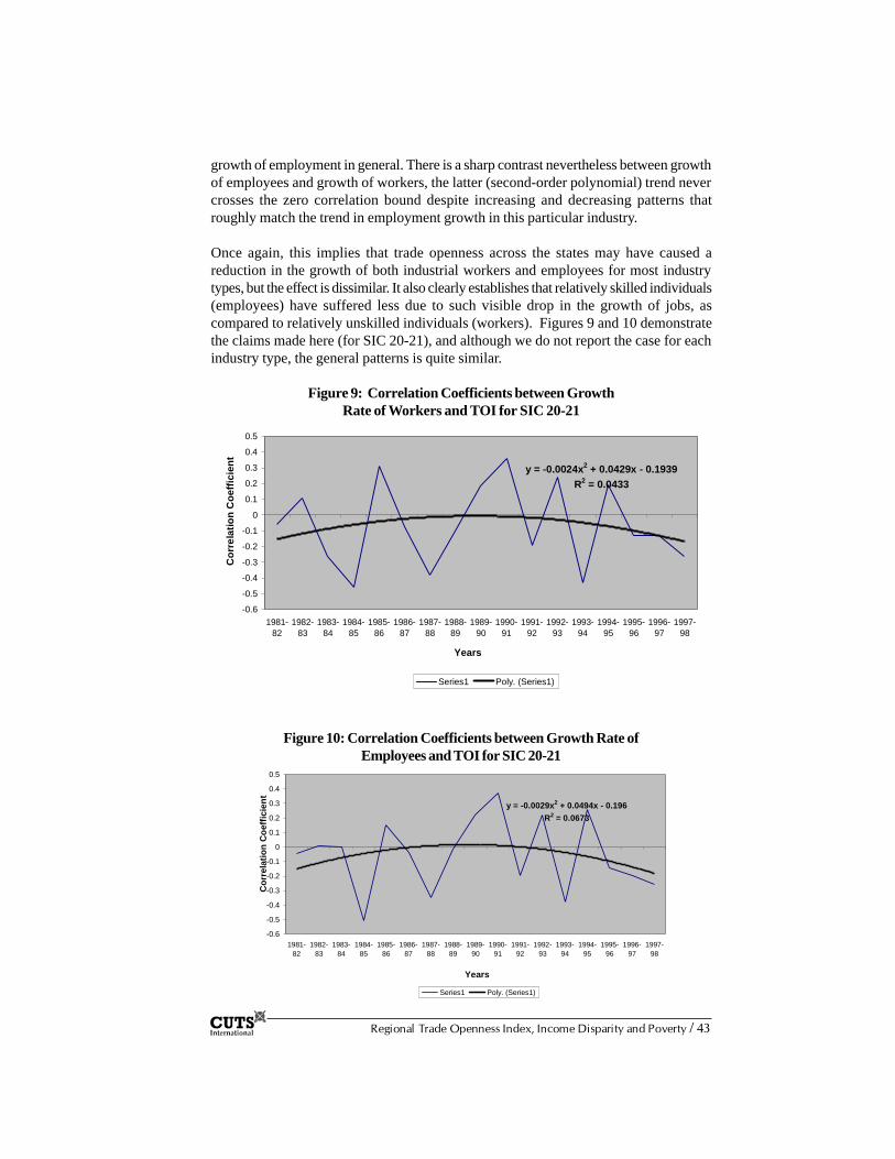
Regional Trade Openness Index, Income Disparity and Poverty / 43
Figure 9: Correlation Coefficients between GrowthRate of Workers and TOI for SIC 20-21
y = -0.0024x2 + 0.0429x - 0.1939R2 = 0.0433
-0.6
-0.5
-0.4
-0.3
-0.2
-0.1
0
0.1
0.2
0.3
0.4
0.5
1981-82
1982-83
1983-84
1984-85
1985-86
1986-87
1987-88
1988-89
1989-90
1990-91
1991-92
1992-93
1993-94
1994-95
1995-96
1996-97
1997-98
Years
Cor
rela
tion
Coe
ffici
ent
Series1 Poly. (Series1)
growth of employment in general. There is a sharp contrast nevertheless between growthof employees and growth of workers, the latter (second-order polynomial) trend nevercrosses the zero correlation bound despite increasing and decreasing patterns thatroughly match the trend in employment growth in this particular industry.
Once again, this implies that trade openness across the states may have caused areduction in the growth of both industrial workers and employees for most industrytypes, but the effect is dissimilar. It also clearly establishes that relatively skilled individuals(employees) have suffered less due to such visible drop in the growth of jobs, ascompared to relatively unskilled individuals (workers). Figures 9 and 10 demonstratethe claims made here (for SIC 20-21), and although we do not report the case for eachindustry type, the general patterns is quite similar.
Figure 10: Correlation Coefficients between Growth Rate ofEmployees and TOI for SIC 20-21
y = -0.0029x2 + 0.0494x - 0.196R2 = 0.0673
-0.6
-0.5
-0.4
-0.3
-0.2
-0.1
0
0.1
0.2
0.3
0.4
0.5
1981-82
1982-83
1983-84
1984-85
1985-86
1986-87
1987-88
1988-89
1989-90
1990-91
1991-92
1992-93
1993-94
1994-95
1995-96
1996-97
1997-98
Years
Cor
rela
tion
Coe
ffici
ent
Series1 Poly. (Series1)

44 / Regional Trade Openness Index, Income Disparity and Poverty
7Openness Index and
Poverty across States in India
This section forms the core of the entire analysis and aims at understanding therelationship between various indices of poverty in the states of India and the
corresponding level of trade openness. It is well known that poverty measurements inIndia are fraught with numerous problems and that the data is not available on acontinuous basis. Therefore, the estimates of poverty that we work with are limited toonly a few entries within the overall time frame we are concerned with. Nevertheless, theavailable data on HCR, Poverty Gap Index (PGI), SPGI and Gini coefficient, may beconsidered sufficient to obtain an overall understanding of the relationship betweeneach of these measures and the state level TOI in India. Methodologically, therefore, webegin by obtaining the data on the said measures of poverty and inequality (PlanningCommission, India) at the state level for the specific time periods during which they werecollected. The data on say, HCR for a particular year and across states is then used toobtain the correlation coefficient with that of the TOI for that particular year and acrossstates.
In Table 12 for example, the correlation coefficient between TOI and Urban HCR for theyear 1983-84 is (0.206) and statistically significant, whereas, the correlation coefficientbetween TOI and rural HCR is 0.217. Figure 11 clearly demonstrates how the correlationcoefficients have changed over time and the trend lines associated with each of the ruraland urban HCR and TOI interaction show a declining trend. In other words, the statespecific trade openness and urban HCR show a trend of negative correlations, i.e.,higher the level of openness lower is the urban HCR or vice versa.
Interestingly, although the rural HCR and TOI coefficients also show a downwardmovement, the slope is rather flat, implying that the negativity of the correlation is notstrong enough. In other words, the TOI does not significantly lower the rural HCRacross states in India, reinforcing the previous conjectures that trade did help the urbanskilled population and other factors of production more than proportionately to theirrural counterpart, which in effect has either directly or by spillovers reduced urbanpoverty more effectively. This again reinforces our primary conjectures on interregionaldisparity owing to greater exposure to international trade in the wake of the process ofliberalisation in India.

Regional Trade Openness Index, Income Disparity and Poverty / 45
Table 12: Correlation between TOI and Urban and Rural HCR, Urban and Rural PG, Urbanand Rural SPG and Urban and Rural GINI
Year Urban Rural Urban Rural Urban Rural Urban RuralHCR HCR PG PG SPG SPG GINI GINI
1983 - 84 0.206 0.217 -0.05 0.103 -0.048 0.118 0.128 -0.153
1986 - 87 0.161 0.511
1987 - 88 0.41 0.33 0.744 0.429 0.744 0.359 0.321 -0.088
1988 - 89 0.576 0.425 0.668 0.394 0.668 0.308 -0.016 -0.243
1989 - 90 0.017 0.579
1990 - 91 0.101 0.328 0.284 0.347 0.284 0.221 0.155 -0.434
1991 - 92 0.149 0.205 0.15 0.067 0.15 -0.07 0.132 -0.569
1992 - 93 0.001 0.156 0.253 0.35 0.253 0.322 0.229 -0.299
1993 - 94 -0.31 0.273 -0.005 0.334 -0.005 0.275 0.209 -0.427
1994 - 95 -0.21 0.048 -0.101 -0.035
1995 - 96 -0.134 0.058 0.236 0.552
1996 - 97 -0.185 0.2 0.18 0.477
1997 - 98 -0.512 0.323
1999 - 00 -0.165 0.439
Figure 11: Correlation Coefficient between Urban and Rural HCR and TOI
-0.6
-0.4
-0.2
0
0.2
0.4
0.6
0.8
1983 -84
1986 -87
1987 -88
1988 -89
1989 -90
1990 -91
1991 -92
1992 -93
1993 -94
1994 -95
1995 -96
1996 -97
1997 -98
1999 -00
Years
Cor
rela
tion
Coe
ffici
ent
Urban HCR Rural HCR Linear (Rural HCR) Linear (Urban HCR)

46 / Regional Trade Openness Index, Income Disparity and Poverty
When it comes to investigating the relationship between urban poverty gap and TOI,the working hypothesis would be that trade lowers the depth of poverty in urbanlocations, which can potentially gain most out of increased trade in goods and servicessimply owing to the larger concentration of such activities in the cities. Figure 12 directlyestablishes that when the correlation trend in rural poverty gap and TOI is increasingthough marginally, the urban trend line is negatively sloped, but less steep compared tothat between urban HCR and TOI.
Figure 12: Correlation between TOI and Urban and Rural Poverty Gap
-0.1
0
0.1
0.2
0.3
0.4
0.5
0.6
0.7
0.8
1983 -84
1986 -87
1987 -88
1988 -89
1989 -90
1990 -91
1991 -92
1992 -93
1993 -94
1994 -95
1995 -96
1996 -97
1997 -98
1999 -00
Years
Cor
rela
tion
Coe
ffici
ent
Urban PG Rural PG Linear (Urban PG) Linear (Rural PG)
This means that with increased openness the depth of poverty has gone up in the ruralareas, i.e., trade exacerbated the poverty problem, in comparison to that in the citieswhere trade has eased the situation in deep pockets of poverty. In fact, in a separateventure, Marjit and Kar (2007) show that in the poet-reform period the marginalisedinformal workers employed in urban non-directory manufacturing enterprises registeran average increase of 10 percent in their real wages across different states in India. Thiscertainly has direct implications for poverty reduction in each state with consequentimpact on the depth of poverty.
Finally, Figures 13 and 14 provide observations on the conditions of the severity ofpoverty (squared poverty gap) and the extent of inequality (Gini coefficient) in rural andurban locations across states in India. Once again, not surprisingly, the impact of greatertrade openness on the urban squared poverty gap is negatively sloped, though evenless steep compared to the previous case, implying that the positive effects of tradeslowly tapers off as one goes deeper down the poverty measurements.
The impact on rural SPGI is almost constant, which is to say, that annual variations in thedegree of openness did not affect the rural SPGI at all. The evidence completely turnsaround when one considers the relationship between TOI and Gini coefficients, wherethe level of inequality within urban locations remains constant despite significantvariations in the state TOI over the years. Interestingly, the same correlation returns apositively sloping curve for the rural counterpart, i.e. the level of rural inequalityunambiguously increased between 1983-84 and 1999-00, as explained by its correlationwith the state level TOI. To sum up therefore, the directional uniformity in all of the

Regional Trade Openness Index, Income Disparity and Poverty / 47
above results indicate that the urban locations in India unambiguously benefited fromthe exposure to increased trade in goods and services as compared to the ruralcounterparts, which suffered not only from an increase in the extent and depth ofpoverty, but also from a higher level of inequality.
Figure 13: Correlation between TOI and Urban and Rural Squared Poverty Gap
-0.2
-0.1
0
0.1
0.2
0.3
0.4
0.5
0.6
0.7
0.8
1983 -84
1986 -87
1987 -88
1988 -89
1989 -90
1990 -91
1991 -92
1992 -93
1993 -94
1994 -95
1995 -96
1996 -97
1997 -98
1999 -00
Years
Cor
rela
tion
Coe
ffici
ent
Urban SPG Rural SPG Linear (Urban SPG) Linear (Rural SPG)
Figure 14: Correlation between TOI and Urban and Rural Gini
-0.8
-0.6
-0.4
-0.2
0
0.2
0.4
0.6
0.8
1983 -84
1986 -87
1987 -88
1988 -89
1989 -90
1990 -91
1991 -92
1992 -93
1993 -94
1994 -95
1995 -96
1996 -97
1997 -98
1999 -00
Years
Cor
rela
tion
Coe
ffici
ents
Urban GINI Rural GINI Linear (Urban GINI) Linear (Rural GINI)

48 / Regional Trade Openness Index, Income Disparity and Poverty
8Concluding Remarks
Our objective has been to devise an openness index and develop a ranking of theIndian states according to their exposure to international trade. This is a proxy
measure since trade data are not available at the regional level. This paper establishedthat states with relatively high levels of income are also the states with greater exposureto trade and such relationship has grown stronger over time. This amounts to thesuggestion that if we pick a relatively affluent state now, the chances that it is fairly openare higher than what would be in early 1980s. We do not establish any causal linkbetween regional prosperity and trade, which is an important future research agenda. Inthe process, we reconfirm general theoretical intuition that exporting states are gettingricher over the years and the import competing states are falling behind. Also a stategenerates higher PCNSDP by switching their production from import competing sectorsto the export sectors.
The openness index thus constructed is applied to two other issues that assumeenormous importance under the present circumstances in India. In section 5, we showthat across various industries trade openness led to significant decline in the rate ofgrowth of employees and workers, where the negative impact on workers is strongercompared to their white collared counterparts. The skill based technological changesand the overwhelming contribution of service sector in the country’s GDP haveunambiguously led to an increased demand for skilled workforce, unlike in the industrialsector in general, where exposure to foreign competition has reduced (slow/negativegrowth) employment opportunities significantly. Consideration of all these factorsmentioned here may be taken up for further explanations in a similar vein. The other issue,which forms the core of all the preceding exercises, is the effect of state level trade opennesson the extent and depth of poverty in India. Here, we find evidences in support of a lowerincidence and depth of poverty for urban locations as compared to rural areas, much to theconformity of other independent studies on economic reforms and poverty. Furthermore,there is clear evidence in support of increasing inequality in the rural areas when thelevel of inequality is correlated with the state level openness index.
One caveat is warranted at the final stage. Our openness is related to export items, whichcommand significant share of total exports, and not those which are outgrowing othersbut remains less significant in terms of overall share. This does not allow us to look at,for example, software related exports. Also it is impossible to find a constant state-wisedata set over time. One could make a separate ranking based on the ‘growth’ in export,which we do not attempt here.

Regional Trade Openness Index, Income Disparity and Poverty / 49
References
Balassa, B. (1982). “Development Strategies in Semi-Industrial Countries”, Oxford: OxfordUniversity Press.
Bardhan, Pranab, (2002). “The politics of economic reform in India”, http://globetrotter.berkeley.edu/macarthur/inequality/papers/BardhanReformIndia.pdf.
Barro, R. J. and Sala-I-Martin, X. (1995)., “Economic Growth”, New York: McGraw-Hill.
Batra, R. (1992). “The fallacy of free trade”, Review of International Economics, Vol. 1,pp.19-31.
Batra, R. and Slottje, D. J. (1993). “Trade policy and poverty in the United States: theoryand Evidence”, 1974-1990', Review of International Economics, Vol. 1, pp.189-208.
Cappelen A., J. Fagerberg and B. Verspagen, (1999). “Lack of Regional Convergence”,in Fagerberg, J., P. Guerrieri and B. Verspagen (Edn.) The Economic Challenge forEurope: Adapting to Innovation-based Growth, Aldershot: Edward Elgar.
Chenery, H. and Strout, A. (1966). “Foreign assistance and economic development”,American Economic Review, Vol. 56, pp.679-733
Clark, B. (1999). “NAFTA: The Effects on Mexico”, Social Science, 410 (November).
Dasgupta, D., P. Maity, R. Mukherjee, S. Sarkar, and S. Chakroborty (2000). “Growth andInter State Disparities in India”, Economic and Political Weekly, Vol.35, No. 27, pp.2413-22.
Datt, Gaurav, (1999). “Has poverty declined since economic reforms? Statistical dataanalysis”, ,Economic and Political Weekly, December 11, 1999.
Datt, Gaurav and Ravallion, Martin. (2002a). “Why has economic growth been morepro-poor in some states of India than others?” Journal of Development Economics,Vol. 68, pp.381-400.
Datt, Gaurav and Ravallion, Martin, (2002b). “Is India’s economic growth leaving thepoor behind?” Journal of Economic Perspectives, Vol.16, No. 3, pp. 89-108.

50 / Regional Trade Openness Index, Income Disparity and Poverty
Datt, Gaurav, Kozel, Valerie and Ravallion, Martin, (2003). “A model-based assessment ofIndia’s progress in reducing poverty in the 1990s”, Economic and Political Weekly,January 25, 2003.
Deaton, Angus and Dreze, Jean, (2002). “Poverty and inequality in India: A Re-examination”, Economic and Political Weekly, September 7, 2002.
Dev, S Mahendra, (1995). “Economic reforms and the rural poo”r, Economic and PoliticalWeekly, August 19, 1995.
Dholakia, R. H. (1994). “Spatial Dimension of Acceleration of Economic Growth inIndia”, Economic and Political Weekly, Vol. 29, No. 35, pp.2303-09
Dholakia, R. H (2003). “Regional Disparity in Economic and Human Development inIndia”, Economic and Political Weekly, Vol. 37, No. 39, pp.4166-72.
Elizondo, R. and P. Krugman, (1992). “Trade Policy and the third world metropolis”,NBER Working Paper, No.4238
Fujita, M., P. Krugman, and A. Venables, (1999). “The Spatial Economy: Cities, Regions,and International Trade”, Cambridge, MA: MIT Press.
Ghosh, B., S. Marjit and C. Neogi, (1998). “Economic Growth, and Regional Divergencein India: 1960 to 1995”, Economic and Political Weekly, Vol. 27, pp.83-116.
Grossman, G. and Helpman, E. (1991). “Innovation and Growth in the Global Economy”,Cambridge: MIT Press.
Hasan, R., D. Mitra and B. P. Ural, (2006). “Trade Liberalisation, Labour MarketInstitutions and Poverty Reduction: Evidence from India States”, forthcoming in IndianPolicy Forum.
Johnson, B. and Sheehy, T. (1996). “Index of Economic Freedom, Washington”, TheHeritage Foundation.
Jones, R. W, H. Beladi and S. Marjit, (1999). “Three Faces of Factor Intensities”, Journalof International Economics, Vol. 48 (2) pp.413-420.
Keesing, D. B. (1967). “Outward-looking policies and economic development”,Economic Journal, Vol. 77, pp.303-20
Krishna, K. L. (2004). “Patterns and Determinants of Economic Growth in IndianStates”, Working Paper No. 144, ICRIER, New Delhi.
Krueger, A. O. (1978). “Foreign Trade Regimes and Economic Development:Liberalisation Attempts and Consequences”, Cambrige, MA, Ballinger.

Regional Trade Openness Index, Income Disparity and Poverty / 51
Krugman, P. (1991). “Increasing Returns and Economic Geography”, Journal of PoliticalEconomy, Vol. 99, No. 3, pp.483-99.
Krugman, P. (1995). “Development, Geography and Economic Theory”, MIT Press.Kurian, N. J. (2000). “Widening Regional Disparities in India: Some Indicators”,Economic and Political Weekly, Vol. 35, No. 7, pp.538-50.
Lall, S. V. and S. Chakravarty, (2006). “Industrial location and special inequality: Theoryand evidence”, in R. Kanbur, A. J. Venbles and G. Wan (Edn.), Special Disparities inHuman Development: Perspective from Asia, United Nations University Press, Tokyo
Leamer, E. (1988). “Measures of openness”, in Baldwin, R. (Edn) Trade Policy and EmpiricalAnalysis, Chicago, University of Chicago Press.
Levine, R. and Renelt, D. (1992). “A sensitivity analysis of cross-country growthregression”, American Economic Review, Vol. 82, pp.942-63
Liu, G. S., X. Liu and Y. Wei, (2001). “Openness and Efficiency of India and ChinaRelative to the World Economy: A Comparative Study”, http://www.brunel.ac.uk/329/efwps/02-18.pdf
Lucas, R. E. (1988). “On the mechanics of economic development”, Journal of MonetaryEconomics, 22(11), pp.3-42
Marjit, S and S. Kar, (2007). “The Urban Informal Sector and Poverty – Effects of TradeReform and Capital Mobility in India”, Poverty and Economic Policy MPIA WorkingPaper (PEP-IDRC) 2007-09. http://www.pep-net.org/
Marjit, S. and S. Mitra, (1996). “Convergence in Regional Growth Rates, Indian ResearchAgenda”, Economic and Political Weekly, Vol.31, No. 33, pp.2239- 42
Marjit, S. and H. Beladi (2005), “International Trade and Interregional Disparity”, CityUniversity of Hong Kong, mimeo.
Mitra, Arup, (2006). “Wages and Employment: Issues and Facts”, Indian Journal ofLabourEconomics, Vol. 49, No. 4, pp.587-602.
Nagaraj, R. (1994). “Employment and wages in manufacturing industries: Trendshypotheses and evidence”, Economic and Political Weekly, Vol. 29, pp.177-186.
Nagaraj, R. (2007). “Labour Market in India Current Concerns and Policy Responses”,OECD Paper.
Romer, P. M. (1986). “Increasing returns and long run growth”, Journal of PoliticalEconomy, 94(5), pp.1002-37.

52 / Regional Trade Openness Index, Income Disparity and Poverty
Romer, P. M. (1992). “Two strategies for economic development: using ideas andproducing Ideas”’, World Bank Annual Conference on Economic Development,Washington, DC, The World Bank.
Sachs, J. and Warner, A. (1995). “Economic reform and the process of global integration”,Brookings Papers on Economic Activity, Vol.1, pp.1-118
Scitovsky, T. (1954). “Two concepts of external economies”, Journal of Political Economy,Vol. 62, pp.143-51
Tapalova, Petia, (2005). “Trade liberalization, poverty and inequality: Evidence fromIndian Districts”’, NBER Working Paper # 11614.
Voivodas, C. (1973). “Exports, foreign capital inflow and economic growth”, Journal ofInternational Economics, Vol.3, pp.337-49.
Wolf, H. (1993). “Trade orientation: measurement and consequences”, Estudios deeconomia, 20(2), pp.52-72
World Bank, (1987). “World Development Report 1987”, Oxford: Oxford UniversityPress.

Regional Trade Openness Index, Income Disparity and Poverty / 53
Annexure
Table A: NIC 1987 and 1998 classifications
Industry 1987 code 1998 code
FOOD, BEVERAGES & TOBACCO 20-22 15-16
TEXTILES 23-26 17-18
WOOD 27 20
PAPER 28 21-22
LEATHER 29 19
CHEMICAL 30 24
RUBBER PLASTICS & PETROLEUM 31 23,25
NONMETAL 32 26
BASIC-METALS 33 27
METAL PRODUCTS 34 28
MACHINARY & EQUIPMENT 35-36 29-33,36
TRANSPORT 37-38 34-35
Source: Summary Statistics, ASI (1997, 1998)
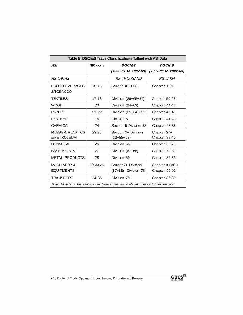
54 / Regional Trade Openness Index, Income Disparity and Poverty
Table B: DGCI&S Trade Classifications Tallied with ASI Data
ASI NIC code DGCI&S DGCI&S
(1980-81 to 1987-88) (1987-88 to 2002-03)
RS LAKHS RS THOUSAND RS LAKH
FOOD, BEVERAGES 15-16 Section (0+1+4) Chapter 1-24
& TOBACCO
TEXTILES 17-18 Division (26+65+84) Chapter 50-63
WOOD 20 Division (24+63) Chapter 44-46
PAPER 21-22 Division (25+64+892) Chapter 47-49
LEATHER 19 Division 61 Chapter 41-43
CHEMICAL 24 Section 5-Division 58 Chapter 28-38
RUBBER, PLASTICS 23,25 Section 3+ Division Chapter 27+& PETROLEUM (23+58+62) Chapter 39-40
NONMETAL 26 Division 66 Chapter 68-70
BASE-METALS 27 Division (67+68) Chapter 72-81
METAL- PRODUCTS 28 Division 69 Chapter 82-83
MACHINERY & 29-33,36 Section7+ Division Chapter 84-85 +
EQUIPMENTS (87+88)- Division 78 Chapter 90-92
TRANSPORT 34-35 Division 78 Chapter 86-89
Note: All data in this analysis has been converted to Rs lakh before further analysis.
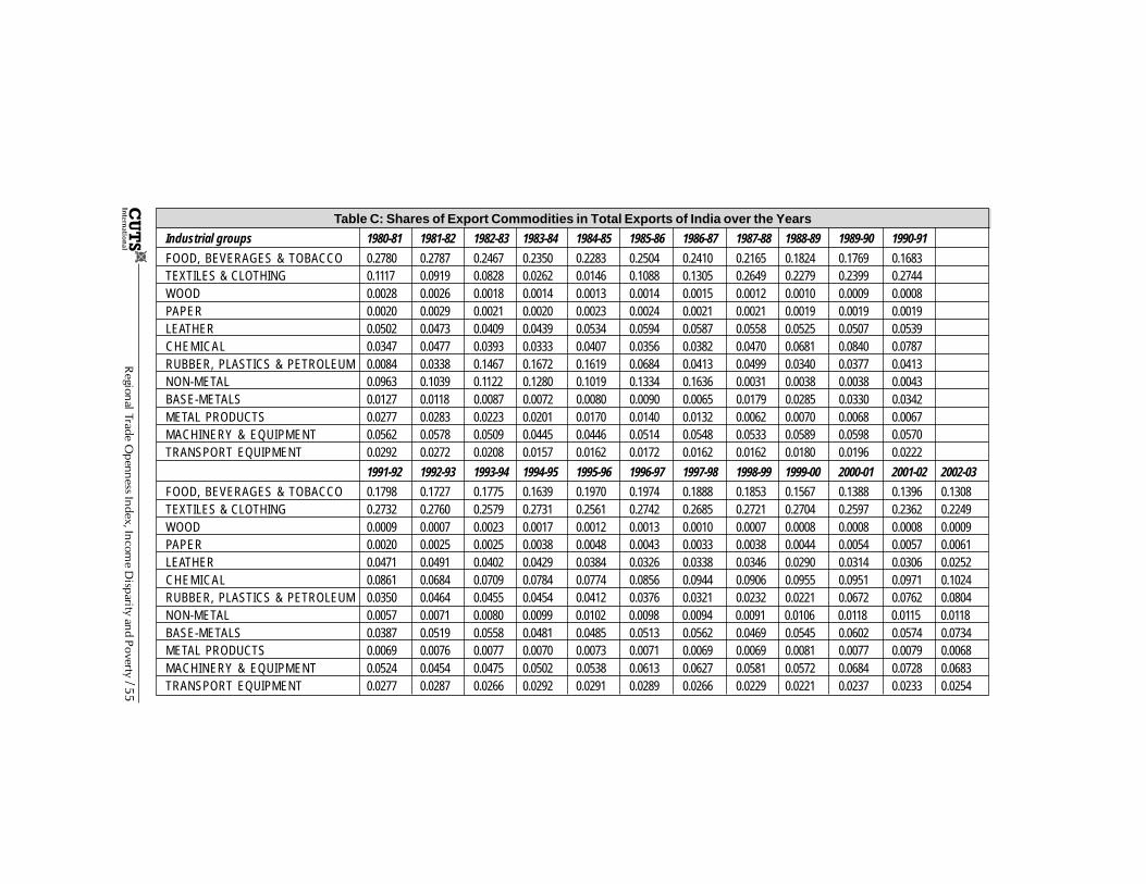
Regional Trade O
penness Index, Income D
isparity and Poverty / 55
Table C: Shares of Export Commodities in Total Exports of India over the Years
Industrial groups 1980-81 1981-82 1982-83 1983-84 1984-85 1985-86 1986-87 1987-88 1988-89 1989-90 1990-91
FOOD, BEVERAGES & TOBACCO 0.2780 0.2787 0.2467 0.2350 0.2283 0.2504 0.2410 0.2165 0.1824 0.1769 0.1683TEXTILES & CLOTHING 0.1117 0.0919 0.0828 0.0262 0.0146 0.1088 0.1305 0.2649 0.2279 0.2399 0.2744WOOD 0.0028 0.0026 0.0018 0.0014 0.0013 0.0014 0.0015 0.0012 0.0010 0.0009 0.0008PAPER 0.0020 0.0029 0.0021 0.0020 0.0023 0.0024 0.0021 0.0021 0.0019 0.0019 0.0019LEATHER 0.0502 0.0473 0.0409 0.0439 0.0534 0.0594 0.0587 0.0558 0.0525 0.0507 0.0539CHEMICAL 0.0347 0.0477 0.0393 0.0333 0.0407 0.0356 0.0382 0.0470 0.0681 0.0840 0.0787RUBBER, PLASTICS & PETROLEUM 0.0084 0.0338 0.1467 0.1672 0.1619 0.0684 0.0413 0.0499 0.0340 0.0377 0.0413NON-METAL 0.0963 0.1039 0.1122 0.1280 0.1019 0.1334 0.1636 0.0031 0.0038 0.0038 0.0043BASE-METALS 0.0127 0.0118 0.0087 0.0072 0.0080 0.0090 0.0065 0.0179 0.0285 0.0330 0.0342METAL PRODUCTS 0.0277 0.0283 0.0223 0.0201 0.0170 0.0140 0.0132 0.0062 0.0070 0.0068 0.0067MACHINERY & EQUIPMENT 0.0562 0.0578 0.0509 0.0445 0.0446 0.0514 0.0548 0.0533 0.0589 0.0598 0.0570TRANSPORT EQUIPMENT 0.0292 0.0272 0.0208 0.0157 0.0162 0.0172 0.0162 0.0162 0.0180 0.0196 0.0222
1991-92 1992-93 1993-94 1994-95 1995-96 1996-97 1997-98 1998-99 1999-00 2000-01 2001-02 2002-03
FOOD, BEVERAGES & TOBACCO 0.1798 0.1727 0.1775 0.1639 0.1970 0.1974 0.1888 0.1853 0.1567 0.1388 0.1396 0.1308TEXTILES & CLOTHING 0.2732 0.2760 0.2579 0.2731 0.2561 0.2742 0.2685 0.2721 0.2704 0.2597 0.2362 0.2249WOOD 0.0009 0.0007 0.0023 0.0017 0.0012 0.0013 0.0010 0.0007 0.0008 0.0008 0.0008 0.0009PAPER 0.0020 0.0025 0.0025 0.0038 0.0048 0.0043 0.0033 0.0038 0.0044 0.0054 0.0057 0.0061LEATHER 0.0471 0.0491 0.0402 0.0429 0.0384 0.0326 0.0338 0.0346 0.0290 0.0314 0.0306 0.0252CHEMICAL 0.0861 0.0684 0.0709 0.0784 0.0774 0.0856 0.0944 0.0906 0.0955 0.0951 0.0971 0.1024RUBBER, PLASTICS & PETROLEUM 0.0350 0.0464 0.0455 0.0454 0.0412 0.0376 0.0321 0.0232 0.0221 0.0672 0.0762 0.0804NON-METAL 0.0057 0.0071 0.0080 0.0099 0.0102 0.0098 0.0094 0.0091 0.0106 0.0118 0.0115 0.0118BASE-METALS 0.0387 0.0519 0.0558 0.0481 0.0485 0.0513 0.0562 0.0469 0.0545 0.0602 0.0574 0.0734METAL PRODUCTS 0.0069 0.0076 0.0077 0.0070 0.0073 0.0071 0.0069 0.0069 0.0081 0.0077 0.0079 0.0068MACHINERY & EQUIPMENT 0.0524 0.0454 0.0475 0.0502 0.0538 0.0613 0.0627 0.0581 0.0572 0.0684 0.0728 0.0683TRANSPORT EQUIPMENT 0.0277 0.0287 0.0266 0.0292 0.0291 0.0289 0.0266 0.0229 0.0221 0.0237 0.0233 0.0254

56 / Regional Trade O
penness Index, Income D
isparity and Poverty
Table D: Share of Import Commodities in Total Imports of India over the Years
Industrial groups 1980-81 1981-82 1982-83 1983-84 1984-85 1985-86 1986-87 1987-88 1988-89 1989-90 1990-91
FOOD, BEVERAGES & TOBACCO 0.0868 0.1014 0.0762 0.1163 0.1017 0.0840 0.0701 0.0864 0.0824 0.0367 0.0342 TEXTILES & CLOTHING 0.0178 0.0258 0.0180 0.0245 0.0202 0.0210 0.0188 0.0203 0.0244 0.0219 0.0208 WOOD 0.0007 0.0012 0.0004 0.0004 0.0005 0.0006 0.0066 0.0108 0.0129 0.0113 0.0106 PAPER 0.0177 0.0226 0.0157 0.0183 0.0241 0.0272 0.0264 0.0267 0.0246 0.0215 0.0241 LEATHER 0.0001 0.0003 0.0002 0.0004 0.0006 0.0004 0.0008 0.0011 0.0018 0.0030 0.0045 CHEMICAL 0.0959 0.0881 0.0596 0.0763 0.1289 0.1298 0.1096 0.0831 0.1098 0.1198 0.1087 RUBBER, PLASTICS & PETROLEUM 0.4354 0.4008 0.4188 0.3269 0.3394 0.2891 0.1808 0.2263 0.2081 0.2325 0.3071 NON-METAL 0.0442 0.0376 0.0591 0.0807 0.0650 0.0611 0.0805 0.0046 0.0057 0.0048 0.0047 BASE-METALS 0.1060 0.1176 0.1061 0.0909 0.0790 0.0347 0.1032 0.1129 0.1257 0.1315 0.1096 METAL PRODUCTS 0.0071 0.0085 0.0010 0.0094 0.0082 0.0103 0.0104 0.0027 0.0025 0.0025 0.0025 MACHINERY & EQUIPMENT 0.1215 0.1379 0.1515 0.1921 0.1719 0.1981 0.2979 0.1976 0.1781 0.1729 0.1599 TRANSPORT EQUIPMENT 0.0376 0.0224 0.0448 0.0282 0.0215 0.0289 0.0400 0.0342 0.0267 0.0422 0.0387
1991-92 1992-93 1993-94 1994-95 1995-96 1996-97 1997-98 1998-99 1999-00 2000-01 2001-02 2002-03
FOOD, BEVERAGES & TOBACCO 0.0287 0.0390 0.0327 0.0614 0.0439 0.0459 0.0516 0.0790 0.0655 0.0439 0.0548 0.0541TEXTILES & CLOTHING 0.0173 0.0221 0.0232 0.0329 0.0266 0.0200 0.0202 0.0201 0.0227 0.0232 0.0298 0.0267WOOD 0.0088 0.0091 0.0062 0.0079 0.0069 0.0070 0.0103 0.0091 0.0093 0.0098 0.0108 0.0068PAPER 0.0185 0.0179 0.0192 0.0180 0.0229 0.0208 0.0224 0.0203 0.0169 0.0182 0.0187 0.0161LEATHER 0.0040 0.0039 0.0050 0.0044 0.0038 0.0037 0.0037 0.0036 0.0032 0.0040 0.0044 0.0035CHEMICAL 0.1341 0.1279 0.1151 0.1310 0.1366 0.1128 0.1222 0.1146 0.1075 0.0847 0.0946 0.0852RUBBER, PLASTICS & PETROLEUM 0.3359 0.3217 0.2984 0.2679 0.2713 0.3213 0.2675 0.2136 0.3103 0.3658 0.3280 0.3408NON-METAL 0.0046 0.0041 0.0038 0.0047 0.0041 0.0033 0.0036 0.0040 0.0035 0.0037 0.0046 0.0040BASE-METALS 0.0840 0.0835 0.0748 0.0899 0.0860 0.0849 0.0752 0.0563 0.0442 0.0405 0.0470 0.0406METAL PRODUCTS 0.0027 0.0026 0.0028 0.0029 0.0027 0.0031 0.0033 0.0037 0.0043 0.0029 0.0027 0.0028MACHINERY & EQUIPMENT 0.1352 0.1408 0.1497 0.1681 0.1928 0.1651 0.1763 0.1630 0.1439 0.1565 0.1681 0.1886TRANSPORT EQUIPMENT 0.0192 0.0211 0.0545 0.0389 0.0302 0.0380 0.0254 0.0189 0.0230 0.0189 0.0224 0.0309

Regional Trade O
penness Index, Income D
isparity and Poverty / 57
Table E: Value of Relative Mean Deviation1980-81 1981-82 1982-83 1983-84 1984-85 1985-86 1986-87 1987-88 1988-89 1989-90 1990-91 1991-92
Andhra Pradesh -15.410 -7.009 -7.449 -10.264 -0.151 -14.610 -18.797 -10.312 -8.450 -6.107 -6.570 -2.979Assam -21.295 -16.907 -14.910 -17.192 -0.188 -18.030 -22.052 -20.828 -30.545 -29.242 -29.973 -28.394Bihar -43.791 -43.874 -44.635 -43.499 -0.397 -41.698 -38.433 -43.372 -44.379 -47.946 -45.711 -49.762Gujarat 18.916 23.513 18.901 31.985 0.287 18.667 23.459 7.108 31.464 23.325 19.780 8.250Haryana 45.274 42.183 47.264 39.646 0.411 57.046 53.238 46.101 57.978 51.777 59.148 59.079Karnataka -6.828 -6.180 -6.087 -6.320 -0.018 -10.756 -4.314 -0.065 -4.992 -4.148 -7.523 2.840Kerala -7.564 -12.936 -12.068 -20.798 -0.173 -18.193 -21.184 -20.073 -22.476 -20.473 -17.682 -16.982Madhya Pradesh -16.759 -19.396 -17.811 -19.615 -0.255 -23.513 -28.670 -21.314 -26.559 -28.962 -23.079 -30.076Maharashtra 49.258 44.672 46.850 45.279 0.436 46.841 44.614 49.984 44.097 59.240 57.969 54.533Orissa -19.456 -23.545 -29.477 -20.741 -0.261 -21.721 -22.106 -26.383 -22.044 -20.753 -37.275 -30.440Punjab 63.908 70.394 72.075 63.587 0.725 76.372 79.113 83.907 69.362 73.979 69.171 73.901Rajasthan -25.095 -23.841 -24.443 -14.094 -0.226 -27.367 -22.540 -30.159 -13.974 -19.960 -11.922 -20.210Tamil Nadu -8.177 -2.801 -9.581 -10.883 -0.013 -2.396 -4.802 -0.928 -4.560 -2.329 1.457 3.204Uttar Pradesh -21.662 -24.375 -20.417 -23.164 -0.240 -25.358 -23.950 -22.716 -23.917 -25.697 -25.075 -26.030West Bengal 8.680 0.103 1.788 6.073 0.062 4.716 6.426 9.050 -1.005 -2.702 -2.715 3.067
1992-93 1993-94 1994-95 1995-96 1996-97 1997-98 1998-99 1999-00 2000-01 2001-02 2002-03Andhra Pradesh -11.206 -4.228 -5.514 -3.305 -3.505 -9.121 -2.587 -2.901 3.860 5.603 3.636Assam -32.196 -26.195 -29.702 -30.992 -34.344 -35.693 -39.660 -40.528 -39.456 -39.618 -39.372Bihar -55.712 -60.780 -59.490 -67.317 -62.168 -65.605 -65.803 -66.270 -60.483 -64.623 -60.549Gujarat 34.606 26.508 41.343 39.561 49.672 44.435 46.322 36.709 27.230 31.713 41.693Haryana 48.977 43.077 42.115 38.315 42.702 37.456 35.595 36.812 40.810 41.160 43.203Karnataka -0.798 1.222 -0.784 0.253 1.890 4.471 12.381 12.180 21.230 14.632 14.990Kerala -15.866 2.513 4.350 4.806 1.856 0.732 2.474 4.634 7.069 6.599 10.994Madhya Pradesh -29.540 -14.973 -19.740 -18.652 -19.656 -18.995 -18.812 -15.207 -26.702 -23.363 -31.634Mahara- shtra 67.092 57.334 48.977 58.395 52.597 54.498 50.594 56.037 44.773 45.858 50.727Orissa -35.724 -36.772 -38.071 -37.653 -45.904 -40.287 -41.716 -41.042 -43.338 -41.002 -43.124Punjab 71.186 64.140 56.647 55.843 55.328 53.244 52.693 52.243 53.300 51.253 48.758Rajasthan -13.993 -20.164 -12.584 -13.548 -10.895 -4.572 -6.741 -12.051 -17.441 -14.683 -25.855Tamil Nadu 2.903 15.647 21.701 21.567 18.448 24.930 23.493 25.226 32.609 26.587 25.125Uttar Pradesh -29.670 -34.577 -36.172 -37.030 -35.330 -38.778 -42.132 -41.658 -43.256 -43.391 -45.327West Bengal -0.058 -12.752 -13.074 -10.242 -10.691 -6.713 -6.102 -4.186 -0.204 3.274 6.735
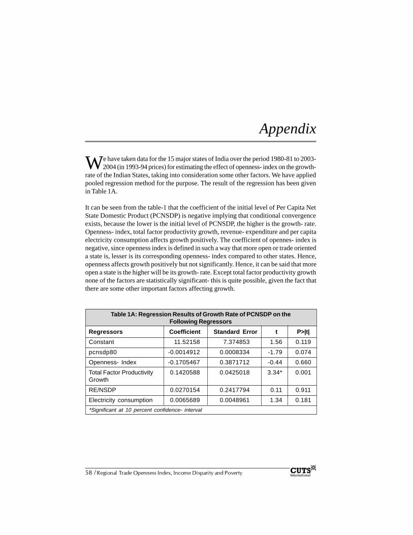
58 / Regional Trade Openness Index, Income Disparity and Poverty
Appendix
We have taken data for the 15 major states of India over the period 1980-81 to 2003-2004 (in 1993-94 prices) for estimating the effect of openness- index on the growth-
rate of the Indian States, taking into consideration some other factors. We have appliedpooled regression method for the purpose. The result of the regression has been givenin Table 1A.
It can be seen from the table-1 that the coefficient of the initial level of Per Capita NetState Domestic Product (PCNSDP) is negative implying that conditional convergenceexists, because the lower is the initial level of PCNSDP, the higher is the growth- rate.Openness- index, total factor productivity growth, revenue- expenditure and per capitaelectricity consumption affects growth positively. The coefficient of opennes- index isnegative, since openness index is defined in such a way that more open or trade orienteda state is, lesser is its corresponding openness- index compared to other states. Hence,openness affects growth positively but not significantly. Hence, it can be said that moreopen a state is the higher will be its growth- rate. Except total factor productivity growthnone of the factors are statistically significant- this is quite possible, given the fact thatthere are some other important factors affecting growth.
Table 1A: Regression Results of Growth Rate of PCNSDP on theFollowing Regressors
Regressors Coefficient Standard Error t P>|t|
Constant 11.52158 7.374853 1.56 0.119
pcnsdp80 -0.0014912 0.0008334 -1.79 0.074
Openness- Index -0.1705467 0.3871712 -0.44 0.660
Total Factor Productivity 0.1420588 0.0425018 3.34* 0.001Growth
RE/NSDP 0.0270154 0.2417794 0.11 0.911
Electricity consumption 0.0065689 0.0048961 1.34 0.181
*Significant at 10 percent confidence- interval

Regional Trade Openness Index, Income Disparity and Poverty / 59
In Table 1A, PCNSDP 80 stands for the Per capita net state domestic product in the year1980-81, Total Factor Productivity growth of the states has been calculated by- (TFP-1)*100 taking 1 as the initial level of Total Factor Productivity (TFP) level of each state.RE/NSDP stands for the Revenue- Expenditure of each state as percentage of Net StateDomestic Product (NSDP) of the corresponding state. Electricity consumption representsper capita electricity consumption of each state.
Besides this, we have found out the correlation- coefficient of Total Factor ProductivityGrowth (TFPG) and Opennes- Index (OI) and have found the correlation to be positive(see Table 2A). The coefficient is negative because the way opennes- index is defined(as explained above). It tells us that openness of a state and its total factor productivitygrowth are positively correlated, which means more open a state is compared to otherstates, its factor productivity will increase faster than others.
We have also run pooled regression of total factor productivity growth on openness-index (Table-3). It can be seen from the table-3 that openness- index affects total factorproductivity growth positively though it is not statistically significant.
Table 2A: Correlation-Coefficient of Total FactorProductivity Growth and Openness Index
OI TFPG
OI 1.0000 -0.0225
TFPG -0.0225 1.0000
Table 3A: Regression Results of Total Factor Productivity Growth (TFPG) onOpenness Index (OI)
Regressors Coefficient Std Eror t P>|t|
Constant 0.7310572 4.058564 0.18 0.857
OI -0.2034836 0.4878859 -0.42 0.677

Regional Trade Openness Index, Income Disparity and Poverty / 71
CUTS Centre for International Trade, Economics & EnvironmentD-217, Bhaskar Marg, Bani Park, Jaipur 302 016, India
Email: [email protected]: www.cuts-international.org; www.cuts-citee.org
ISBN 978-81-8257-102-0