regional impact models - rrirri.wvu.edu/webbook/schaffer/regionalgt.pdf · regional impact models...
TRANSCRIPT

Regional ImpactModels
by
William A. SchafferProfessor of Economics
Georgia Institute of Technology
July 1999
© 1999 Regional Research Institute, West Virginia University.
No portion of this document may be reproduced on paper or electronically withoutexpress permission from the Regional Research Institute.

© 1999 RRI, WVU i July 1999
PREFACE
This survey of regional input-output models and their use in impact analysis has evolved fromover twenty years of experience in constructing regional economic models and in teaching aboutthem. My objectives are to present this family of models in an easily understood format, to showthat the models we use in economics are well-structured, and to provide a basis for understandingapplications of these models in impact analysis. I have tried to present the models in such a waythat understanding the logic and algebra of the simplest economic-base model leads to anunderstanding of the only slightly more complex regional and interregional input-output models incommon use today. The advanced models become matrix-algebra extensions of the simple models.
I have greatly benefited from the guidance of Professor Kong Chu over the years. He firstintroduced these models to me in 1967 and has helped with interpretations and tedious explanationsof mathematical points until only recently; now he teaches me about life and philosophy. I am indebt to a number of Georgia Tech students as well. While they have been assistants and students intitle, they have been my best teachers as well. To name a few: Richard Dolce was my firstprogrammer; Malcolm Sutter spent three years with me programming models in Hawaii and forGeorgia; Clay Hamby maintained Sutter's programs and helped with several impact studies; LarryDavidson, now Professor of Economics at Indiana, has remained a colleague for over 25 years;Ross Herbert spent two summers in Nova Scotia thrashing out a completely new system; SteveStokes had the pleasure of reconstructing both the Hawaii and Nova Scotia models; and JohnMcLeod continues to improve my computing skills and graphics and managed data collection andorganization in a recent study of amateur sports in Indianapolis with Davidson. In addition, Johnconverted this document to its HTML format. Thanks to all of these, to a set of astute butanonymous reviewers, and to Scott Loveridge, the Regional Research Institute, and West VirginiaUniversity for making this experiment in electronic publication possible.
I would appreciate your reporting of all errors of communication and expression in thisdocument.
William A. Schaffer
June 1999

© 1999 RRI, WVU ii July 1999
TABLE OF CONTENTS
PREFACE..............................................................................................................................I
TABLE OF CONTENTS .................................................................................................II
LIST OF FIGURES ..........................................................................................................V
LIST OF ILLUSTRATIONS .........................................................................................V
LIST OF TABLES .............................................................................................................V
1 INTRODUCTION ...............................................................................................................1
2 REGIONAL MODELS OF INCOME DETERMINATION : SIMPLEECONOMIC -BASE THEORY .........................................................................................2
ECONOMIC-BASE CONCEPTS....................................................................................................2Antecedents...............................................................................................................................2Modern origins.......................................................................................................................... 3
THE STRUCTURE OF MACROECONOMIC MODELS....................................................................3THE "STRAWMAN" EXPORT-BASE MODEL...............................................................................5THE TYPICAL ECONOMIC-BASE MODEL...................................................................................6TECHNIQUES FOR CALCULATING MULTIPLIER VALUES..........................................................8
Comparison of planner's relationship and the economist's model......................................................... 8The survey method..................................................................................................................... 8The ad hoc assumption approach................................................................................................... 9Location quotients...................................................................................................................... 9Minimum requirements............................................................................................................. 10"Differential" multipliers: a multiple regression analysis................................................................. 10
CRITIQUE: ADVANTAGES, DISADVANTAGES, PRAISE, CRITICISM...........................................11STUDY QUESTIONS.................................................................................................................11
3 INPUT-OUTPUT TABLES AND REGIONAL INCOME ACCOUNTS ...................14INTRODUCTION.......................................................................................................................14THE REGIONAL TRANSACTIONS TABLE..................................................................................14INCOME AND PRODUCT ACCOUNTS.......................................................................................17SUMMARY ..............................................................................................................................19STUDY QUESTIONS.................................................................................................................19APPENDIX 1 CD-ROM DATA SOURCES.................................................................................20APPENDIX 2 MEASURES OF REGIONAL WELFARE................................................................21
The problem with GSP estimates................................................................................................ 21The widespread use of personal income estimates............................................................................ 21
4 THE LOGIC OF INPUT -OUTPUT MODELS ..............................................................22INTRODUCTION.......................................................................................................................22THE RATIONALE FOR A MODEL: ANALYSIS VS. DESCRIPTION...............................................22PREPARING THE TRANSACTIONS TABLE: CLOSING WITH RESPECT TO HOUSEHOLDS..........22THE ECONOMIC MODEL..........................................................................................................23

© 1999 RRI, WVU iii July 1999
Identities: the transactions table.................................................................................................. 23Technical conditions: the direct-requirements table......................................................................... 24Equilibrium condition: supply equals demand................................................................................. 25Solution to the system: the total-requirements table........................................................................ 26
ECONOMIC CHANGE IN INPUT-OUTPUT MODELS...................................................................29Causes vs. consequences of change.............................................................................................. 29Structural change...................................................................................................................... 29Changes in final demand............................................................................................................ 30
STUDY QUESTIONS.................................................................................................................30
5 REGIONAL INPUT -OUTPUT MULTIPLIERS ...........................................................33INTRODUCTION.......................................................................................................................33THE MULTIPLIER CONCEPT....................................................................................................33
An intuitive explanation............................................................................................................ 33The iterative approach............................................................................................................... 34
MULTIPLIER TRANSFORMATIONS..........................................................................................37Output multipliers.................................................................................................................... 37Employment multipliers............................................................................................................ 37Income multipliers................................................................................................................... 39Government-income multipliers.................................................................................................. 39
STUDY QUESTIONS.................................................................................................................39APPENDIX 1 MULTIPLIER CONCEPTS, NAMES, AND INTERPRETATIONS...............................43
Introduction............................................................................................................................. 43Income multipliers................................................................................................................... 43Employment multipliers............................................................................................................ 46Output multipliers.................................................................................................................... 47Observations and summary......................................................................................................... 47Further extensions.................................................................................................................... 47
6 INTERREGIONAL MODELS ........................................................................................50INTERREGIONAL ECONOMIC-BASE MODELS..........................................................................50
Review of one-region models...................................................................................................... 50Two-region model with interregional trade..................................................................................... 50
EXTENSIONS AND FURTHER STUDY.......................................................................................52Interregional interindustry models................................................................................................ 52Economic-ecologic models......................................................................................................... 52
STUDY QUESTIONS.................................................................................................................52
7 COMMODITY -BY-INDUSTRY ECONOMIC ACCOUNTS : THE NOVASCOTIA INPUT -OUTPUT TABLES ............................................................................53
INTRODUCTION.......................................................................................................................53A SCHEMATIC SOCIAL-ACCOUNTING FRAMEWORK..............................................................53
Commodity accounts................................................................................................................ 53Industry accounts...................................................................................................................... 56Final accounts......................................................................................................................... 56
AGGREGATED INPUT-OUTPUT TABLES...................................................................................56The commodity flows table........................................................................................................ 59The commodity origins table...................................................................................................... 59
STUDY QUESTIONS.................................................................................................................59
8 COMMODITY -BY-INDUSTRY INTERINDUSTRY MODELS : THE LOGICOF THE NOVA SCOTIA INPUT -OUTPUT MODEL ................................................62
INTRODUCTION.......................................................................................................................62THE DATA ...............................................................................................................................62TECHNICAL CONDITIONS........................................................................................................62

© 1999 RRI, WVU iv July 1999
The constant-imports assumption................................................................................................ 63The constant market-share assumption.......................................................................................... 63The constant-technology assumption............................................................................................ 65Equilibrium condition: supply equals demand................................................................................. 67Solution: the total-requirements table........................................................................................... 67
ECONOMIC CHANGE IN COMMODITY-BY-INDUSTRY MODELS...............................................68STUDY QUESTIONS.................................................................................................................69APPENDIX 1 THE MATHEMATICS OF THE UNITED STATES INPUT-OUTPUT MODEL..............72
9 BUILDING INTERINDUSTRY MODELS ....................................................................74THE BASIC MODEL..................................................................................................................74ESTIMATING TECHNIQUES......................................................................................................74
Survey-only techniques.............................................................................................................. 75The supply-demand pool procedure............................................................................................... 75Export-survey method............................................................................................................... 76Selected-values method.............................................................................................................. 77
COMMODITY-BY-INDUSTRY PROCEDURES............................................................................77RIMS.................................................................................................................................... 77IMPLAN................................................................................................................................ 77IO7........................................................................................................................................ 77IOPC..................................................................................................................................... 77Others.................................................................................................................................... 77
STUDY QUESTIONS.................................................................................................................77
ANSWERS TO SELECTED QUESTIONS......................................................................78
REFERENCES.....................................................................................................................80

© 1999 RRI, WVU v July 1999
LIST OF FIGURES
FIGURE 3.1 THE TRANSACTIONS TABLE AS A PICTURE OF THE ECONOMY..................................15FIGURE 4.1 ALGEBRAIC TRANSACTIONS TABLE............................................................................24FIGURE 5.1 THE ACTIVITY EFFECT OF $100 SALE TO FINAL DEMAND BY THE MANUFACTURING
SECTOR....................................................................................................................................34FIGURE 5.2 THE MULTIPLIER EFFECT OF $100 SALE TO FINAL DEMAND BY THE
MANUFACTURING SECTOR......................................................................................................35FIGURE 5.3 THE RIPPLE EFFECT OF A $100 EXPORT OF MANUFACTURING OUTPUT..................36
LIST OF ILLUSTRATIONS
ILLUSTRATION 2.1 THE SIMPLE KEYNESIAN MODEL.....................................................................4ILLUSTRATION 2.2 THE PURE EXPORT-BASE MODEL.....................................................................6ILLUSTRATION 2.3 THE PURE ECONOMIC-BASE MODEL................................................................7ILLUSTRATION 4.1 THE SIMPLE INPUT-OUTPUT MODEL..............................................................32ILLUSTRATION 7.1 SCHEMATIC INPUT-OUTPUT TABLE FOR NOVA SCOTIA................................54ILLUSTRATION 7.2 SCHEMATIC INPUT-OUTPUT TABLE FOR NOVA SCOTIA EMPHASIZING THE
COMMODITY ACCOUNTS.........................................................................................................55ILLUSTRATION 7.3 SCHEMATIC INPUT-OUTPUT TABLE FOR NOVA SCOTIA EMPHASIZING THE
INDUSTRY ACCOUNTS.............................................................................................................57ILLUSTRATION 7.4 SCHEMATIC INPUT-OUTPUT TABLE FOR NOVA SCOTIA EMPHASIZING THE
FINAL INCOME AND EXPENDITURE ACCOUNTS......................................................................58ILLUSTRATION 8.1 THE SIMPLE COMMODITY-BY-INDUSTRY INPUT-OUTPUT MODEL FOR A
REGION.....................................................................................................................................70
LIST OF TABLES
TABLE 3.1 HYPOTHETICAL INTERINDUSTRY TRANSACTIONS......................................................14TABLE 3.1 HYPOTHETICAL INTERINDUSTRY TRANSACTIONS......................................................14TABLE 3.2 INCOME AND PRODUCT ACCOUNTS FOR GEORGIA, 1970 ...........................................18TABLE 4.1 HYPOTHETICAL INTERINDUSTRY TRANSACTIONS WITH ENDOGENOUS HOUSEHOLD
SECTOR....................................................................................................................................23TABLE 4.1 HYPOTHETICAL INTERINDUSTRY TRANSACTIONS WITH ENDOGENOUS HOUSEHOLD
SECTOR....................................................................................................................................23TABLE 4.2 HYPOTHETICAL DIRECT-REQUIREMENTS TABLE........................................................25TABLE 4.3 TOTAL REQUIREMENTS (WITH HOUSEHOLDS ENDOGENOUS).....................................27TABLE 4.4 INDUSTRY-OUTPUT MULTIPLIERS (WITH HOUSEHOLDS ENDOGENOUS).....................27

© 1999 RRI, WVU vi July 1999
TABLE 4.5 TOTAL REQUIREMENTS (WITH HOUSEHOLDS EXOGENOUS) .......................................28TABLE 4.6 A COMPARISON OF OUTPUT MULTIPLIERS UNDER DIFFERENT HOUSEHOLD
ASSUMPTIONS..........................................................................................................................28TABLE 5.1 HYPOTHETICAL DIRECT-REQUIREMENTS TABLE........................................................33TABLE 5.2 THE MULTIPLIER EFFECT OF $100 IN MANUFACTURING OUTPUT TRACED IN ROUNDS
OF SPENDING THROUGH THE HYPOTHETICAL ECONOMY.......................................................35TABLE 5.3 OUTPUT, EMPLOYMENT, INCOME, AND LOCAL AND STATE GOVERNMENT REVENUE
MULTIPLIERS FOR HYPOTHETICAL ECONOMY........................................................................38TABLE 5.4 SUMMARY OF MULTIPLIER NAMES AND FORMULAS FROM MILLER AND BLAIR,
INPUT-OUTPUT ANALYSIS.......................................................................................................49TABLE 7.1 AGGREGATED COMMODITY FLOWS, NOVA SCOTIA, 1984..........................................60TABLE 7.2 AGGREGATED COMMODITY ORIGINS, NOVA SCOTIA, 1984........................................61TABLE 8.1 AGGREGATED COMMODITY-BY-INDUSTRY PROVINCIAL FLOWS, NOVA SCOTIA, 1984
.................................................................................................................................................64TABLE 8.2 DOMESTIC MARKET-SHARE COEFFICIENTS, NOVA SCOTIA, 1984.............................65TABLE 8.3 PROVINCIAL INTERINDUSTRY TRANSACTIONS, NOVA SCOTIA, 1984 ........................66TABLE 8.4 DIRECT REQUIREMENTS PER DOLLAR OF GROSS OUTPUT, NOVA SCOTIA, 1984......67TABLE 8.5 TOTAL REQUIREMENTS (DIRECT, INDIRECT, AND INDUCED), NOVA SCOTIA, 1984....68TABLE 8.6 INDUSTRY-OUTPUT MULTIPLIERS, NOVA SCOTIA, 1984 ............................................68

© 1999 RRI, WVU 1 Draft July 28, 1999
1 INTRODUCTION
This document introduces the reader towhat has come to be known as "regionalimpact analysis." This form of analysistypically emphasizes the regional benefitsassociated with changes in structure of aregional economy and is normally based ondemand-oriented models of local economies.
Our intention is to introduce the reader tothe family of models known as regionalinput-output models. And a primary objectiveis to show that the models we use ineconomics are well-structured. I have tried topresent the models in such a way thatunderstanding the logic and algebra of thesimplest economic-base model leads to anunderstanding of the only slightly morecomplex regional input-output models andinterregional models. The advanced modelsbecome matrix-algebra extensions of thesimple models and are remarkably painless tounderstand.
Chapter 2 starts with the simplest model inregional economics -- the economic-basemodel -- and develops a pattern of modelconstruction which will be followed in allsucceeding models.
Chapter 3 presents the regional input-output table as a description of the economyusing on simple accounting conventions.
Chapter 4 develops the logic of input-output models in an easily understoodextension of the logic of economic-basemodels.
Chapter 5 focuses on regional input-outputmultipliers and thus is the chapter of mostconcern for analysts interested solely ininterpretation of impact analyses.
Chapter 6 is a brief extension intointerregional models. Here the methods ofinput-output analysis are applied to economicbase models to point toward the interpretationof interregional input-output models.
Chapter 7 lays out the commodity-by-industry format in common use inconstructing input-output tables since 1970.
This is the format in which data is nowcurrently available at the national level.
Chapter 8 builds the input-output model inindustry-by-industry terms from the tablespresented in Chapter 7. These two chaptersparallel Chapters 3 and 4 in developing thelogic of the model.
Finally, Chapter 9 provides a briefdiscussion of ways to build input-outputmodels using nonsurvey techniques. It isrelatively generic and has not yet beenextended to cover the various commerciallyavailable systems.

© 1999 RRI, WVU 2 Draft July 28, 1999
2 REGIONAL MODELS OF INCOMEDETERMINATION: SIMPLE ECONOMIC-BASE
THEORY
Economic-base conceptsEconomic-base concepts originated with
the need to predict the effects of neweconomic activity on cities and regions. Say anew plant is located in our city. It directlyemploys a certain number of people. In amarket economy these employees depend onothers to provide food, housing, clothing,education, protection and other requirementsof the good life. The question which cityplanners and economists need to answer, then,is "what are the indirect effects of this newactivity on employment and income in thecommunity?" With these estimates in hand,we can work toward planning the socialinfrastructure needed to support all of thesepeople.
Economic-base models focus on thedemand side of the economy. They ignorethe supply side, or the productive nature ofinvestment, and are thus short-run inapproach. In their modern form, they are inthe tradition of Keynesian macroeconomics.In an introductory economics course, wemight start with a simple model of a closedeconomy, usually with some unemployment.In regional economics we deal with an openeconomy with a highly elastic supply oflabor.
It is appropriate to start this chapter firstwith a look at the place of economic-basetheory in the history of economic thought andthen twith a review the simple Keynesianmodel and the elementary economic-basemodels. We will then look at methods ofestimating the values of multipliers.
Antecedents
It is common to divide economies into twoparts. In action, it's us against them; inprimitive life, it is hunters and gatherers; inanalysis, it will be primary against secondary,productive and nonproductive, basic andnonbasic, export and support, fillers and
builders, productive and sterile workers,necessary and surplus labor, etc. Thefollowing notes trace obvious antecedents.1
Mercantilistic thought is a prime example.During the period in which the mercantilistswere dominant, normally considered to befrom 1500 to 1776, the nation-states ofEurope were consolidating their power andgaining strength to resist or conquer others.The writers who documented the timesemphasized a philosophy not unlike that of amodern merchant or chamber of commerce.
The mercantilists stressed accumulating asupply of gold with which to pursue thenation's political and military objectives. Theeconomic base of a nation included thesectors which created a favorable balance oftrade. Goods were produced for exportdespite the needs of a poor population, exportof unprocessed materials was prohibited,shipping in local bottoms was forcedwhenever possible, and colonies wereexploited as a source of raw materials.
Thomas Mun, a merchant in the Italian andNear Eastern trade and a director of the EastIndia Company, was probably the mostfamous of these writers. His exposition ofmercantilist doctrine in England's Treasureby Foreign Trade, written in 1630, explainedhow "… to enrich the kingdom and toencrease our Treasure." He emphasized asurplus of exports as the key:
Although a Kingdom may be enriched by giftsreceived, or by purchase taken from some otherNations, yet these are things uncertain and of smallconsideration when they happen. The ordinarymeans therefore to encrease our wealth and treasureis by Forraign Trade, wherein wee must everobserve this rule; to sell more to strangers yearly
1 This section is based on (Oser 1963) and (Kang andPalmer 1958). Oser's The Evolution of EconomicThought is one of the best short histories of economicthought in print.

Economic-Base Theory Chapter 2
© 1999 RRI, WVU 3 July 1999
than wee consume of theirs in value.(from Oser1963 p.14)
The Physiocrats, led by François Quesnayand briefly prominent in France in the secondhalf of the 18th century prior to the FrenchRevolution, responded to the excesses of themercantilists with several points important tolater thought. They considered societysubject to the laws of nature and opposedgovernmental interference beyond protectionof life, property, and freedom of contract.They opposed all feudal, mercantilist, andgovernment restrictions. "Laissez faire,laissez passer," the theme phrase for the freeenterprise system, is from the Physiocrats.They opposed luxury goods as interferingwith the accumulation of capital.
But, for our purposes, they wereprecursors of economic-base thought in twoways. First, they were important in theirtreatment of the sources of value. To thePhysiocrats, only agriculture was productive.The soil yielded all value; manufacturing,trade, and the professions were sterile, simplypassing value on to consumers. Thisclassification of productive and sterileactivities is similar to the basic and serviceclassification in economic-base discussions.
And second, the Physiocrats visualizedmoney flowing through the economic systemin much the same way as blood flows throughthe living body. Quesnay's tableaueconomique was a predecessor of thecircular-flow diagrams popularized inKeynesian macroeconomics.
Adam Smith, writing in 1776, and heavilyinfluenced by these French authors, took aless extreme but nevertheless strong position.He emphasized production of material ortangible goods and considered service andgovernment as unproductive.
Karl Marx, in das Kapital, also divided theeconomy into two parts. To Marx, necessarylabor was the source of wealth and was paidfor with a wage barely sufficient to maintainits provider. Surplus labor was also providedby workers but its value was appropriated bythe capitalists in the form of surplus value.Workers had to produce not only what theyconsumed but also a surplus for the capitalist.Menial servants, landlords, the Church, and
commercial activities were unproductive –they added nothing to total value.
Others of the nineteenth century were moregenerous. Jean Baptiste Say in his Treatiseon Political Economy (1803) popularizedAdam Smith in France. Say's famous Law ofMarkets, paraphrased as "supply creates itsown demand," required that all work beproductive, that all compensated activitycreates utility.
Nevertheless, we can see a strong line ofthought dividing economic activities into twoparts, and we can see economic-base conceptsas fitting into a centuries-old pattern.
Modern origins
Modern literature on the economic basehas been voluminous, but plaguedoccasionally by scholastic sloppiness inappropriate citations.
It seems that Werner Sombart, a Germaneconomic geographer writing in the early partof this century, should receive major credit formodern concepts.1
Sombart was responsible for thedistinction between "town fillers" and "townbuilders," ("Städtegründer" and“Städtefüller") which appeared in FrederickNussbaum's A History of the EconomicInstitutions of Modern Europe (with fullpermission). But in a series of articles in theearly 1950's, Richard B. Andrews quotedextensively from Nussbaum withoutmentioning the fact that Nussbaum had basedhis book on Sombart's work. Andrew's workwas widely circulated and became thestandard reference.
The structure of macroeconomicmodels
It is convenient to begin with a review ofthe basic elements of model building. Wecan start with the simplest of allmacroeconomic models, the Keynesian modelof a closed economy. This model ispresented algebraically in Illustration 2.1 and
1 I rely on Günter Krumme for this statement (Krumme1968).

Economic-Base Theory Chapter 2
© 1999 RRI, WVU 4 July 1999
follows the standard format we will use in allof our models: we outline definitions,behavioral or technical assumptions,equilibrium conditions, and finally the
solution. Since this is a process we willfollow with each new model considered, itmay be worthwhile to review the nature ofthese model elements.
Illustration 2.1 The simple Keynesian model
Definitions or identities:Planned Expenditures ≡ Consumption + Investment (Planned sources of income)
(1) E ≡ C + I Actual Income (output) ≡ Consumption + Savings (Actual disposition of income)
(2) Y ≡ C + S
Behavioral or technical assumptions:Consumption = A linear function of income (Both planned and actual)
(3) C = a + cY (c < 1 = the marginal propensity to consume)Investment = Planned investment (an exogenously determined value)
(4) I = I'
Equilibrium condition:Income = Expenditures, or actual income is equal planned expenditures
(5) Y = E or, with C + I = C + S, we can subtract C from both sides to form an equivalent equilibrium condition:Drains = Additions
(6) I = S
Solution by substitution:Y = C + I Substitute (1) into (5)Y = a + cY + I' Substitute (3) and (4)
Y - cY = a + I' Gather the Y, or income, terms(1 - c)Y = a + I' Factor out YY = {1/[1 - c]}*(a + I') Isolate Y through division
The simple Keynesian investment multiplier is:dY/dI = 1/[1 - c]
A definition is a statement of fact. Bydefinition, it is always true. In mathematics,the proper term is identity. One of the moreimportant identities in macroeconomics is thenational income identity: realized nationalincome (actual expenditures) is the sum ofrealized consumption and realized investment.In the simple national model, this has to be atrue statement—it is a tautology. Actualexpenditures have to equal their sum!
Another important identity in the simplemodel is that income (which is another termfor 'output') is equal to the sum of
consumption and savings. We, as recipientsof incomes, either spend our incomes or wesave (don't spend). This identity can also betaken as a definition of saving as thedifference between income and consumption.
Behavioral assumptions are equationsdescribing the behavior of certain groups, oractors, in the economy. In this case, the keybehavioral relationship is the consumptionfunction, which postulates consumption asdependent on, or caused by, income:
C = f(Y)

Economic-Base Theory Chapter 2
© 1999 RRI, WVU 5 July 1999
which in its linear form may be expressed as:
C = a +cY
where a represents autonomous consumptionand c is the marginal propensity to consume(dC/dY). The parameters of the equation area and c. Recall that if a>0, dC/dY<C/Y.
An incidental but important result of thisassumption is that saving is also a function ofincome:
S ≡ Y - C = -a + (1 - c)Y
The other important behavioral assumptionin this simple model is that investment, I, isdetermined outside the system. It is planned.In terms common to model building, it is anexogenous variable in contrast toconsumption, which is determinedendogenously (that is, 'within the system').
(An example of a technical assumption isthe production function. A productionfunction describes the relations betweeninputs and outputs. A familiar example isQ=F(K,L), commonly used to describe howcapital and labor are combined to produceoutput.)
Equilibrium is a condition in which theexpectations (plans) of decision-makers(actors) in the system are met. In this simplemodel, the equilibrium condition is thatincome equals planned expenditures, or, whatis the same thing, that saving (which sets thelimits on actual investment) equals plannedinvestment.
The point is that planned investment andsaving do not have to be equal (even thoughin the end, actual saving has to equal actualinvestment—this is a fundamental principle ofaccounting). When they are equal, then allparties are satisfied. When they are not,forces are at play which will take income to alower or higher level, bringing saving intoequality with planned investment.
Good introductions to the art of model-building can be found in several readilyavailable books (e.g. Bowers and Baird 1971;Kogiku 1968; Neal and Shone 1976). Thesimple Keynesian model is outlined in almost
all texts on the Principles of Economics. Agood reference is (Case and Fair 1994).
The "strawman" export-base modelIt is common in economics to construct a
"strawman" against which to rail and argue.Nowhere is this practice more common thanin the regional literature. The "export-base"model, in which the sole determinant ofeconomic growth is exports, is often built torepresent the arguments of other practitioners.However, you can seldom find an "export-base" theorist who is not also an "economic-base" theorist who admits to many otherdeterminants of growth than exports alone.
Now let us construct this strawman and seehow a pure export-base stance is untenable.We move into an open economy and makeexports the sole exogenous factor. If anyautonomous expenditure is included (theeasiest is for consumption), then regionalincome can exist even when exports are zero(Ghali 1977).
The model differs only slightly from thesimple Keynesian model. With Keynes, thekey leakage was savings. He explained theunderemployment of a depressed economy asresulting when planned investment fell belowfull-employment equilibrium levels due to alack of confidence in investment markets.His endogenous variable was consumption,through which most income flowsoccurred—the flows became disconnected inthe saving-investment path.
In the export-base model, the endogenousflow remains consumption, redefined now as“domestic expenditures.” We completelyignore saving and hide investmentexpenditures within domestic expenditures(we are concerned not about explainingdepression in the whole economy but aboutexplaining changes in regional income). Thefunction of saving in creating a leakage fromthe economy is now assumed by imports,which is defined as a function of income.The function of investment is now assumedby exports, the driver of the export-basedeconomy.

Economic-Base Theory Chapter 2
© 1999 RRI, WVU 6 July 1999
Illustration 2.2 The pure export-base modelDefinitions or identities:
Total expenditures ≡ domestic production + exports (inflows)(1) E ≡ D + X
Income ≡ Domestic expenditures +Imports(2) Y ≡ D + M, or D ≡ Y - MBehavioral or technical assumptions:
Imports = a linear function of income(3) M = mY (m<1,the marginal propensity to import)
Exports = an exogenously (outside-region) determined value(4) X = X'Equilibrium condition:
Income = Total expenditures(5a) Y = E
orDrains = Additions
(5b) M = XSolution by substitution:
Y = Y - M + X Substitute (1) and (2) into (5a)Y = Y - mY + X' Substitute (3), and (4)Y - Y + mY = X' Gather the Y, or income, termsmY = X' Factor out YY = (1/m)*X' Isolate Y through division
The export-base multiplier is:dY/dX = 1/m
This model obviously stresses opennessand dependence of the region on eventsbeyond its reach.
The typical economic-base modelTo make the model slightly more realistic
(or, rather, less simplistic!), saving and
exogenously determined investment can beadded back into the system. Illustration 2.3includes these to develop an almost typicaleconomic-base model. Only minorinterpretive comments are required.

Economic-Base Theory Chapter 2
© 1999 RRI, WVU 7 July 1999
Illustration 2.3 The pure economic-base model
Definitions or identities:Total expenditures ≡ Domestic production + Exports + Investment
(1) E ≡ D + X + IIncome ≡ Consumption + Saving
(2) Y ≡ C + SConsumption ≡ Domestic expenditures + Imports
(3) C ≡ D + M, or D ≡ C - MBehavioral or technical assumptions:
Consumption = a linear function of income(4) C = cY (c = the marginal propensity to consume)
Imports = a linear function of income(5) M = mY (m = the marginal propensity to import)
Exports = an exogenously (outside-region) determined value(6) X = X'
Investment = an exogenously (outside-system) determined value(7) I = I'Equilibrium condition:
Income = Total expenditures(8a) Y = E
orDrains = Additions
(8b) M + S = X + ISolution by substitution:
Y = C - M + X + I Substitute (1) and (3) into (8a)Y = cY - mY + X' + I' Substitute (4), (5), (6) and (7)Y - cY + mY = X' + I' Gather the Y, or income, terms(1 - c + m)Y = X' + I' Factor out YY = {1/[1 - (c - m)]}*(X' + I') Isolate Y through division
The economic-base and investment multipliers are:dY/dX = 1/[1 - (c - m)], and dY/dI = 1/[1 - (c - m)]

Economic-Base Theory Chapter 2
© 1999 RRI, WVU 8 July 1999
The missing element is autonomousconsumption (which appeared in the simpleKeynesian model). Whether or not it isincluded seems to me to be a matter ofpersonal preferences. On the one hand, itmight be nice to be complete and consistentwith the Keynesian model. In addition, itserves to warn us that the consumptionfunction is probably curvilinear, originating atthe origin and rising at a decreasing rate withrespect to income. The marginal propensityto consume at the range of incomes overwhich we might work is less than the averagepropensity to consume. A positiveautonomous consumption permits us tosimulate this case.
On the other hand, we already have oneexogenously determined nonexport variable,investment. The investment multiplier isidentical to that which would be calculated forautonomous consumption—we have theresults without the bother. While this is alogic which might reduce a model to pulp ifpursued too rigorously, I have leftautonomous consumption out of thisillustration.
Techniques for calculatingmultiplier values
Comparison of planner's relationshipand the economist's model
Concentrating purely on the practical needto develop an easy way to forecast communitychange, early planners developed economic-base ratios (T/B for the average ratio, and∆T/∆Β for the marginal ratio, where the lettersrepresent total (T) and basic (B) income oremployment) by pure observation as rules ofthumb. By 1952, economists (Hildebrandand Mace 1950) had developed export-basemodels in the same analytic framework as theKeynesian macroeconomists, with multipliersexpressed as (1/(1-PCL), where PCLrepresents either the average propensity toconsume locally produced goods (APCL) orthe marginal propensity (MPCL). Couldthese approaches be equivalent? Yes.Charles M. Tiebout showed us how (Tiebout1962). Tracing the metamorphosis foraverage propensities,
T/B = 1/(B/T) = 1/((T-NB)/T)) = 1/(1-NB/T)= 1/(1-APCL)
Here, the ratio of nonbasic activity to totalactivity (NB/T) is the equivalent of the averagepropensity to consume locally producedgoods.
So, if we can obtain values of total andbasic variables over a period of years, we canestimate marginal export-base multipliers byregressing the total on the basic values. Withthe regression line formulated as T = a +bB,the slope b is the marginal multiplier (∆T/∆Β)for the region.
The survey method
Of course, the most straight-forwardmethod is simply to ask businesses in thearea to specify how much of their revenues isbasic and to use their responses to accuratelydivide local business activities into basic andservice components. In practice, this isseldom done.
The neglect of the survey approach is easyto explain. It is the most expensive and time-consuming of approaches. Questionnaires onsensitive issues such as revenues,employment, and markets are seldomanswered freely; to obtain even a smatteringof responses the study team must resort topersonal interviews. And even then, theinterviewers must be skilled and persuasive.
In addition, if the area is of any size, thesurvey would require careful planning. Acanvass would be prohibitive and the samplemust be carefully stratified and selected torepresent the broad spectrum of activitiesrepresented in modern communities. Suchcare and expense would meet the test ofrationality only if data collection were in thecontext of a much larger study. The limit tothe value of a simple export-base ratio isfairly low, in the hundreds of dollars.
A final argument against this simpleapproach is that the survey would probablyyield data for only one year, leading tocalculation of an average multiplier when amarginal multiplier is the most appropriate.

Economic-Base Theory Chapter 2
© 1999 RRI, WVU 9 July 1999
The ad hoc assumption approach
The easiest and least expensive of methodsis simply to rely on arbitrary assignment ofactivities to basic or nonbasic categories.This could be done by assignment of, say,employment or payrolls for entire industriesinto categories, or it could be accomplishedwith a little more finesse by estimatingproportions of employment involved in basicactivities.
Needless to say, the chance of errors islarge even for experienced analysts, and themultiplier will again be an average one withlimited use in analyzing the effect of change.
Location quotients
The location quotient is probablyresponsible for the long-life and continuingpopularity and use of economic-basemultipliers. These quotients provide acompelling and attractive method forestimating export employment (or income).
A location quotient is defined as the ratio
LQi = (ei/e)/(Ei/E),
where ei is area employment in industry i, e istotal employment in the area, Ei isemployment in the benchmark economy inindustry i, and E is total employment in thebenchmark economy. Normally, the"benchmark" economy is taken to be thenation as the closest available approximationto a self-sufficient economy.
Assuming that the benchmark economy isself-sufficient, then a location quotient greaterthan one means that the area economy hasmore than enough employment in industry ito supply the region with its product. And aquotient less than one suggests that the area isdeficient in industry i and must import itsproduct if the area is to maintain normalconsumption patterns.
Surplus or export employment in industryi can be computed by the formula
EXi = (1 - 1/LQi)*ei , LQi > 1,
which is easily shown to be the differencebetween actual industry employment in the
area and the "necessary" employment in thearea.
In fact, then, excess employment can becomputed without reference to locationquotients through this reduction of theformula:
EXi = ei - (Ei/E)*e
It is convenient to retain the initial formula asa reminder of the logic, and to computelocation quotients as reminders of thestrengths of exporting industries.
Now it is easy to estimate exportemployment for each industry in the area andto sum these estimates to yield a value forexport employment for the area in someparticular year. With this number and totalemployment, an average multiplier for the areacan be computed. With a set of these valuesover 10-20 years, the more acceptablemarginal multiplier can be estimated bysimple regression.
While it is common to use employment asthe primary basis for these calculations, othermeasures such as wages and salaries are justas appropriate. Indeed, wage data is moreaccessible electronically, especially on CD-ROM. County Business Patterns, a standardsource of employment and payroll data, isavailable for years since 1986, two years perdisk. In considerable detail, this is the bestdata for recent years, but skill with mainframecomputers, tapes, and programming isrequired to gain access for earlier years.The Regional Economic Information System(REIS), updated on CD-ROM annually by theU.S. Department of Commerce with a two-year lag, includes a relatively aggregated 10-category employment series for the years1969-96 as well as a more detailed earningsseries for every county in the nation. Thisdata makes earnings-based location quotientsa snap, especially if historic estimates aredesired.
Location quotients have been in use byregional analysts for over 40 years now, andhave been commented on at length. Weshould look at the assumptions involved intheir use as well as the advantages anddisadvantages.

Economic-Base Theory Chapter 2
© 1999 RRI, WVU 10 July 1999
The literature records at least three specificassumptions: (1) that local and benchmarkconsumption patterns are the same, (2) thatlabor productivity is a constant acrossregions, and (3) that all local demands are metby local production whenever possible. Thefirst assumption is not serious: not only canwe not discern differences in consumptionpatterns without extraordinary expense but wecan suspect that differences in productionpatterns are more important. Purchases ofintermediate goods by producers differ forregions depending on industry mix. (It turnsout that we can account for industry mix withinput-output models, so this difference hasbeen accounted for by the march of time.).
The constant-labor-productivityassumption is difficulty to avoid. Its impactcan be ameliorated slightly through usingearnings data, which can be assumed to reflectregional productivity variation throughdifferences in wage rates. (This assumptioncould in turn be attacked if wages vary moreby area cost-of-living than by productivity.)
The assumption that local demands are metfirst by local production is the more tenuousof the three. It is obviously not true, as anyvisit to a grocery or clothing store will attest.But it is common, and a better alternative ishard to come by.
In addition to the disadvantages accruingfrom these assumptions, another major faultis that the method is dependent on the degreeof aggregation of the data, makingcomparisons among various studies of littlevalue. To illustrate the problem, consider thefood and kindred products industry inAtlanta. The location quotient computed forthis broad industry should be less than one,and if excess employment were computedbased on this classification, none would becredited to the food industry. But if theclassification were more detailed, the soft-drink industry would show a large number ofexcess employees, since the headquarters ofCoca-Cola is in the city.
The overpowering advantages of usinglocation quotients are that the method isinexpensive and the exercise of computingexcess employment may give the analyst anopportunity to gain insights of interest inthemselves.
Minimum requirements
In the 1960's, when available computingtechnology favored frequent use of economic-base models, one of the alternatives to the useof location quotients was the minimum-requirements approach (Ullman and Dacey1960). This variation involved a slightrevision of the location-quotient formula to
EXi = ei - (Ei/E)
min
*e ,
where (Ei/E)min
is the minimum employmentproportion for industry i in cities of sizesimilar to the subject city. You can readilysee that we have substituted a varyingbenchmark employment proportion for aconstant one:
LQi = (ei/e)/(Ei/E)min
.
While still appearing in various forms inthe literature, the method suffers from twomajor criticisms. One is that, if enough citiesare included in the selected set, all regions willbe exporting and none may be importing.The other is similar in that, if we use datadefined in a fine level of detail (which seemsan improvement, and was one in location-quotient estimates) we may reduce local needsto near zero and make almost all productionfor export (Pratt 1968).
At any rate, the method is not commonlyused now. The location-quotient methodremains the virtually sole survivor as a simplemeans of identifying export industries.
"Differential" multipliers: a multipleregression analysis
Another approach which has been used inestimating economic-base multipliers is to fita multiple regression equation to regionaldata. The first of these studies arose in astudy of the impact of military bases onPortsmouth, New Hampshire in 1968 byWeiss and Gooding (Weiss and Gooding1968).
Simple economic-base models ignore thepossibility that different industries may havedifferent impacts on their community. Theregression technique eliminates thissimplifying assumption. Weiss and Goodingset up an equation

Economic-Base Theory Chapter 2
© 1999 RRI, WVU 11 July 1999
S = Q + b1 X1 + b2 X2 + b3 X3,
where S represents service employment, Q isa constant, and the X terms are, in order,private export employment, civilianemployment at the Portsmouth NavalShipyard, and employment at Pease Air ForceBase.
With data fitted from 1955-64, their resultswere
S = -12905 + .78 X1 + .55 X2 + .35 X3 (.31) (.23) (.14)
The multipliers are 1+ bi for each sector.
Weiss and Gooding used a mixture ofassumption and location quotient methods inallocating export employment and assumedthat the export sectors were independent andthat workers in the export sectors demandedsimilar services.
This variation on economic-base modelinghas not fallen into widespread use for severalreasons: its flexibility (in number ofexogenous sectors) is limited by the numberof observations available, otherwise thecoefficients may not be significant;determining the export content of industryemployment remains a demanding chore; andwith the rise of desktop computing, input-output models are better sources of industry-specific multipliers and are similar in cost.
Critique: advantages,disadvantages, praise, criticism
Economic-base models suffer from oldage: they have been built by so manyanalysts with varying levels of quality andthey have been criticized so often that littleremains except the concept.
The indictment would include thefollowing phrases:
Short run
Nonspatial
Simple adaptations of national models
Data is normally available for administrative units(counties) which may be poorly defined aseconomic regions.
Ignores capacity constraints
Assumes perfect elasticity of supply for inputs
Pits the area against the rest of the world, showingno interdependence between regions
Multiplier varies with size of region. (As a regiongrows it diversifies, importing less and soincreasing local consumption and the multiplier(Sirkin 1959)). Also, larger regions tend toinfluence neighbors more and so to enjoy largerfeedback effects (Richardson 1972)
An employment multiplier is often used to discussincome changes. (But this assumes thatemployment and per capita income are perfectlycorrelated -- in a simple economy with perfectlyelastic supplies of labor this might be the casealthough, of course, the world is not simple.)
Assumes that exports are the sole determinant ofeconomic growth. (It is not reasonable for us totake the rap for this.) Any rational person can seethat the determinants of growth are many -- thesimple model just emphasizes one determinant.Perhaps the fault lies in early attempts to formulatemultipliers and the ease with which the simplemultipliers could be constructed. (Ghali 1977;Sirkin 1959))
Direction of dependence may be questionable:which comes first, export growth or a strongservice sector, or interdependence? Should we beconcerned with preconditions for export growth(setting up an attractive service sector) in thissimple model? Are we planning growth orexplaining the true basis?
Although castigated for decades, theeconomic-base model has survived as a verysuccinct expression of the power of demandin regional income determination. The mostcurrent, and perhaps the clearest and mostcomplete, statement of its status is found in arecent review by Andrew J. Krikelas (1992),available from the Federal Reserve Bank ofAtlanta or in .pdf format from the School ofEconomics web site at Georgia Tech(http://www.econ.gatech.edu/faculty/schaffer/.
Study questions1. Outline a simple export-base model and compare
it with the simple Keynesian model of nationalincome determination.
2. Criticize the export-base model, then note itsvirtues.
3. Justify classifying the minimum-requirementsmethod for computing export-base multipliers as

Economic-Base Theory Chapter 2
© 1999 RRI, WVU 12 July 1999
a special variation of the location-quotientmethod.
4. Outline the methods commonly used inestimating export-base multipliers, noting theiradvantages and disadvantages.
5. The "pure economic-base model" outlined inIllustration 2.3 does not include any reference toautonomous consumption. Assume that totalexpenditures include autonomous consumptionexpenditures, that the marginal propensitiesremain linear, and that imports are a linearfunction of total expenditures. Rebuild the"pure" model as a "typical" model under theseassumptions. How has the multiplier changed?
6. Collect data from an electronic source foravailable years and use location quotients toestimate export employment in a county.
7. Construct the economic model on which theequation estimated to determine "differentialmultipliers" is based.
8. Rebuild the models in Illustrations 2.1-3 withthe equilibrium condition stated as "Drains =Additions."
9. Build the economic model behind the estimatingequation T = a - bB.
10. Which should be the best, an average multiplieror a marginal multiplier?
11. In Illustration 2.3, the alternative formulation ofthe equilibrium condition is M+S=X+I . Lay outthe full model using these variables.
12. Complete the exercise on the following page.

Economic-Base Theory Chapter 2
© 1999 RRI, WVU 13 July 1999
Exercise
EXPORT-BASE MULTIPLIER CALCULATIONS
You are the planner/economist for a simple 3-industry community and need to produce a multiplierestimate for a report due this afternoon. Answer the following questions and do the calculations.
State the formulas for the location quotient and export employment for an industry:
LQi =
EXi =
Data and calculations
Employment Empl. proportions Location ExportIndustry Local National Local National quotient employment
Year 1
1 10 80 ______ ______ ______ ______
2 4 20 ______ ______ ______ ______
3 2 60 ______ ______ ______ ______
Total 16 160 1.00 1.00
Year 2
1 16 100 ______ ______ ______ ______
2 6 25 ______ ______ ______ ______
3 2 75 ______ ______ ______ ______
Total 24 200 1.00 1.00
Multipliers
Concept In words In numbers Value
Average multiplier, year 2 = ___________________ = ____________ = _______
Marginal multiplier, years 1-2 = ___________________ = ___________ = _______

© 1999 RRI, WVU 14 Draft July 28, 1999
3 INPUT-OUTPUT TABLES AND REGIONAL INCOMEACCOUNTS
IntroductionThis chapter presents the input-output table
as an accounting system for an economy.Labeled “hypothetical”, the numeric exampleis actually a 5-industry aggregation of thedetailed table for Georgia in 1970 (Schaffer1976). (Although out-of-date, it fits the styleof most regional input-output tables in currentuse in the United States. It also fits the text,which is a slight revision of that used toexplain the Georgia system.) First we look atthe table as a whole; then we examine in moredetail the quadrant of the table which reportsthe income and product accounts for thisregional economy.
The regional transactions tableA regional input-output model traces the
interactions of local industries with eachother, with industries outside the region, and
with final demand sectors. The centralelement in this model is a regionaltransactions table such as that shown in Table3.1. This table records transactions betweenfive broad industries, three final-paymentssectors, and three final-demand sectors. (Theoriginal presentation was of transactionsbetween 50 industries, six final-paymentssectors, and 6 final-demand sectors.)
Each row in this table accounts for thesales by the industry named at its left to theindustries identified across the top of the tableand to the final consumers listed in the right-hand section of the table. Intermediate goodsare sold to local industries for use inproducing other products while finishedgoods are sold to final consumers. Goodsexported from the region to other parts of thenation and the world are listed under exportsin the final-demand section, regardless oftheir stage of production. The sum of a rowis the total output or total sales of an industry.
Table 3.1 Hypothetical interindustry transactions
Buying Con- Manu- Total Household Other lo- Total
Industry Extrac- struc- fac- Ser- industry expendi- cal final final Total
Selling tion tion turing Trade vices demand tures demand Exports demand demand
industry ( 1 ) ( 2 ) ( 3 ) ( 4 ) ( 5 ) ( 6 ) ( 7 ) ( 8 ) ( 9 ) ( 1 0 ) ( 1 1 )
Extraction ( 1 ) 1 8 3 3 1 5 9 9 6 7 3 8 9 2 9 9 8 8 5 9 6 7 8 2 1 6 7 4
Construction ( 2 ) 1 4 1 4 3 1 4 2 9 3 3 6 4 0 1 8 0 3 3 5 3 2 1 5 5 2 5 2 0
Manufacturing ( 3 ) 1 4 2 4 1 4 1 3 9 0 1 1 0 3 5 6 2 4 1 2 1 2 7 5 1 1 3 0 9 3 4 4 1 1 7 5 0 1 4 1 6 2
Trade ( 4 ) 5 2 2 2 4 5 2 0 7 2 2 5 7 1 1 2 6 2 5 6 3 1 6 1 9 7 0 3 6 9 5 4 8 2 0
Services ( 5 ) 1 0 2 2 2 1 8 6 2 5 5 8 1 9 9 0 3 7 3 3 4 2 6 2 5 2 3 2 8 2 8 7 6 1 3 1 1 3 4 7
Total local inputs ( 6 ) 4 9 3 8 9 1 3 4 1 5 7 6 0 2 9 6 9 8 5 2 7 8 1 9 9 3 7 0 5 1 4 0 9 1 2 5 9 9 5 3 4 5 2 3
Households ( 7 ) 5 9 5 6 6 5 3 6 9 6 2 3 8 5 4 6 0 3 1 1 9 4 4 1 0 0 2 5 2 4 0 2 6 2 3 1 4 5 6 7
Other payments ( 8 ) 2 6 1 1 9 1 1 6 2 4 1 3 6 5 2 4 0 2 5 8 4 2 (3789.2) (943.2) 1097.5) 0 5 8 4 2
Imports ( 9 ) 3 2 5 7 7 3 5 4 2 8 3 1 1 1 3 7 2 8 2 0 9 3 7 7 8 1 0 5 7 - 1 2 9 9 4 - 8 1 5 9 5 0
Total final payments ( 1 0 ) 1 1 8 1 1 6 2 9 1 0 7 4 7 4 0 6 0 8 3 7 8 2 5 9 9 5 3 8 7 8 3 5 8 1 - 1 2 9 9 4 - 5 5 3 6 2 0 4 5 9
Total inputs ( 1 1 ) 1 6 7 4 2 5 2 0 1 4 1 6 2 4 8 2 0 1 1 3 4 7 3 4 5 2 3 1 2 0 7 7 7 2 8 5 1 0 9 7 2 0 4 5 9 5 4 9 8 2

I/O Tables and Regional Accounts Chapter 3
© 1999 RRI, WVU 15 July 1999
Thus, sales by the extraction industry (acombination of agricultural, forestry, fishing,and mining industries) are shown in row oneof Table 3.1. Of the total output worth $1,674million, over 35 percent is sold to lightmanufacturing (which processes it for furthersale), and over 35 percent is sold outside theregion. The remaining sales are largely toother industries within the broad extractiveindustry itself.
Each column in Table 3.1 records thepurchases, or inputs, of the industry identifiedat the top of the column from the industriesnamed at the left. Payments by the industryto employees, holders of capital, andgovernments are contained in the first tworows of the final-payments section of thetable. These payments constitute the "valueadded" by the industry in question.Purchases from industries outside the regionare identified in the last row of the final-payments section and are called "imports."These imports may be either of goods notproduced at all in the region or of goods
produced in quantities insufficient to meetlocal needs. The sum of the entries in eachcolumn represents the total purchases by theindustry in question. Since profits, losses,depreciation, taxes, etc., are recorded in thetable as final payments, the total purchasesand payments must equal total sales. Inputsequal outputs; hence the term "input-output."
For example, the purchases and paymentsof the extractive industry are shown incolumn 1 of Table 3.1. Since this industry isalmost 90 percent agriculture, the columnreflects large intraindustry transactions(purchases of feeder stocks, baby chicks,grains, etc.), substantial purchases from lightmanufacturing (feeds), and a large payment tohouseholds for labor and proprietors' income.Local farmers also import from outside thestate large amounts of feeds and othersupplies. Notice that the total inputs is thesame as the total outputs identified in row 1.
Figure 3.1 The transactions table as a picture of the economy
II
Interindustry
s truct ure
I
Consump-
t ion
pat terns
III
Incomes
IV
Nonmarke t
t ransfers
Final DemandsProduction
Total inputs

I/O Tables and Regional Accounts Chapter 3
© 1999 RRI, WVU 16 July 1999
Now, with this brief introduction to a regionaltransactions table, let us look at the table as anaccounting system for an economy. Figure3.1 shows an input-output table in skeletonform and divided into four quadrants.Quadrant I describes consumer behavior,identifying consumption patterns ofhouseholds and such other local final users ofgoods as private investors and governments.Another important part of Quadrant I is theexport column, which shows sales to otherindustries and consumers outside the regionaleconomy. Since these goods would notnormally reappear in the region in the sameform, these sales are regarded as final.According to economic-base theory, in whichfinal demand is the motivating force in aneconomy, we would look in this quadrant foractivity-generating forces and we wouldespecially examine the government and exportsectors.
Quadrant II depicts productionrelationships in the economy, showing theways that raw materials and intermediategoods are combined to produce outputs forsale to other industries and to ultimateconsumers. This is the most importantquadrant in an input-output table. Forregions, it typically ranges in size between 30and 500 industries. Quadrant II is the basisfor the input-output model itself.
Quadrant III shows incomes of primaryunits of the economy, including the incomesof households, the depreciation and retainedearnings of industries, and the taxes paid tovarious levels of government. Thesepayments are also called value added; sincethey are so hard to identify individually, theseincomes are frequently recorded as one value-added row. The quadrant also includespayments to industries outside the economyfor materials and intermediate goods whichare imported into the region. Since all ofthese payments to resource owners and tooutsiders leave the industrial system of theregion, they are called "final payments."
Quadrant IV identifies primarilynonmarket transfers between sectors of theeconomy and might properly be labeled the"social transfers" quadrant. Here we seegifts, savings, and taxes of households; wesee the surpluses and deficits of governments
and their payments to households andintergovernmental transfers. The quadrantalso typically includes purchases by final-demand sectors from industries outside theregion.
Now, to make a major point about thehazards of aggregation, let's look at the tableas originally presented, as a picture of theGeorgia economy in 1970. Out of a totaloutput of over $34 billion, Georgia'smanufacturing output in 1970 was valued atover $14 billion and its service output at over$11 billion, indicating that Georgia'seconomy was dominated by themanufacturing and service industries. Evenso, Georgia was not a major manufacturing orservice economy by national standards, as canbe seen in the following comparison of theindustrial origins of value added in Georgiaand the United States (Schaffer 1976)
Percent of value addedSector Georgia U.S.
Agriculture, mining 4.2 5.2Construction 4.4 5.6Manufacturing 26.0 28.9Transportation, utilities 7.7 8.1Trade 18.3 14.6Services 25.6 26.9Government 13.7 10.7
Georgia had larger contributions to valueadded from trade and government than did thenation, and smaller contributions from theextractive industries, construction,manufacturing, utilities, and services. Thisdeviation from the national pattern is anexpression of the region's modest stage ofdevelopment and its central position in theSoutheast.
But this observation also shows that the"importance" of an industry is completelydependent on the definitions and aggregationpatterns employed in constructing a table. Byenlarging the table and altering sectordefinitions, we could change the apparentimportance of industries. For example, bycombining the agricultural industries with thefood-processing industry (normally inmanufacturing) we could make the"agriculture-based" industry larger than anyof the components of the "trade" or "service"

I/O Tables and Regional Accounts Chapter 3
© 1999 RRI, WVU 17 July 1999
industries. In fact, in the 29-industry version(not shown here) of the Georgia table, the fivelargest industries in terms of output are: 1)trade, 2) finance, insurance and real estate, 3)services, 4) textile mill products, and 5)transportation equipment.
A second interesting item in Table 3.1 isthe gross product of Georgia. Analogous inconcept to the gross national product, grossregional product (GRP) can be defined astotal production without duplication, or as theeconomic product of all factors of productionresiding in the region. It can also be seen asthe total final payments (adjusted for imports)in the region, 20.459 billion dollars.Alternatively, it is also the total final demandby ultimate consumers of the region'sproducts (net of imports).
In summary, an input-output table tracesthe paths by which incomes flow through theeconomy. Quadrant I is where the spendingcycle begins and is where finished goods goto satisfy the needs of final consumers.Quadrant III is where the production cyclestarts, with households and other resourceowners, including governments, receivingpayments for their contributions to theproduction process. Quadrant II tracesproduction relationships, describing thetechnology of production in the economy. Itoutlines the market sector of the economy.Quadrant IV identifies nonmarket flows ofmoney, showing purchases of labor inputs bygovernments, taxes paid by households,surpluses and deficits of governments, andtransfers between governments and othergovernments and people.
Income and product accountsThe input-output table embodies not only
measures of gross regional product but also asummary set of social, or income and product,accounts for the region. Like the input-outputtable itself, these accounts are part of adouble-entry accounting system for theeconomy. In the same way that abusinessman uses his accounts to develop aconsolidated income statement for his firm,the economist uses income and productaccounts to measure the performance of theeconomy and to compare the behavior ofparts of the economy against other standards.
Table 3.2 is the transactions table rearrangedto emphasize Quadrant IV, the sector in whichsocial accounts are traced. This social-accounts table completely ignores the flowsof intermediate products through theproduction quadrant and suppresses thedetails of the other quadrants. It emphasizes(1) the total final payments to resourceowners for their contributions to production,(2) the aggregate demand for final products,and (3) the transfers which take place betweenprimary units of the economy.
We have slightly rearranged the table. Therow showing purchases from nonlocalindustries (imports) has been moved abovethe final-payments rows. A row for transfersto households has been added to account fornonproductive money transfers to persons.And the one row for other payments in Table3.1 has been expanded into four to show thedetails of final payments and transfers.
Six accounts are outlined in the table. Thereceipts side of the household account isshown in the household-income andhousehold-transfers rows, which total to bepersonal income; the payments side isdetailed in the household-expenditurescolumn. The saving and investment accountis shown in the capital-residual row (retainedearnings, depreciation, savings) and theinvestment column. Local, state, and federalgovernment accounts are shown in their rowsand columns. And the rest-of-the-worldaccount is shown in the row labeled"purchases from nonlocal industry" and thecolumn "net exports." By placing theseaccounts into one matrix, we gain botheconomy in presentation and a feeling fortheir commonality.
Gross state product (GSP) may bemeasured in two ways, the incomes approachand the expenditures approach. Let us startwith the expenditures approach.

I/O Tables and Regional Accounts Chapter 3
© 1999 RRI, WVU 18 July 1999
Table 3.2 Income and product accounts for Georgia, 1970Sales to House-
Account pro- hold Private Expenditures of governments Total
receiving\making cessing expendi- invest- Federal, Federal, Net final Totalpayment sectors tures ment Local State defense other exports demand receipts
Purchases from
local processors 8,527.2 8,199.3 1,400.4 460.9 432.3 1,057.0 353.9 14,091.3 25,995.1 34,522.3
Purchases from
nonlocal industry 8,159.3 3,777.8 802.1 138.8 115.8 -12,993.8 -8,159.3 0.0
Total purchases
from industry 16,686.5 11,977.1 2,202.5 599.7 548.1 1,057.0 353.9 1,097.5 17,835.8 34,522.3
Household
income 11,882.6 99.7 790.7 372.7 671.0 689.3 2,623.4 14,506.0
Total purchases of
goods and services 28,569.1 12,076.8 2,202.5 1,390.4 920.8 1,728.0 1,043.2 1,097.5 20,459.2 49,028.3
Household
transfers 61.0 51.3 190.7 209.0 848.0 1,299.0 1,360.0
Capital
residual 3,019.1 871.6 -1,688.2 -816.6 2,202.5
Local govern-
ment income 480.3 377.9 445.9 47.3 112.4 983.5 1,463.8
State govern-
ment income 858.8 341.9 22.1 408.8 -55.2 717.6 1,576.4
Federal govern-
ment income 1,533.9 2,197.8 19.1 533.5 2,750.4 4,284.3
External
transfers
Totaloutlay 34,522.2 15,866.0 2,202.5 1,463.8 1,576.5 1,937.0 2,347.3 0.0 25,393.1 59,915.3
Using expenditures, we define GSP asstate output at market value as measuredthrough the expenditures of final consumers.This approach accounts for the final demandfor Georgia's product by four groups ofconsumers: households, investors,governments, and private units outside thestate economy. In Table 3.2, GSP is seen astotal purchases of goods and services for finalconsumption, $20,459 million. In 1970, thiswas 2.1 percent of GNP. In comparison toexpenditures for GNP, Georgia spent less ofher gross product on personal consumption(59.0 percent in contrast to 62.9 percent forthe nation), less on private investment (10.7,13.5), and less on local and state government(11.3, 12.2); she made up for this in terms offederal defense expenditures (8.4, 7.5), otherfederal expenditures (5.0, 3.6), and net privateexports (5.3, 0.4).
Using incomes, we can arrive at a similarGSP by adding the "income receipts" of thevarious accounts. The major receipt is earnedhousehold or personal income, which consistsof wages and salaries, other labor income,proprietors' income, and property incomes.
Including business transfer payments(primarily bad debts) and social securitycontributions, this amounts to $14,567million, or 71.2 percent of GSP; thecorresponding national figure is 75.2 percent.The "capital residual," or gross businesssaving, of processors is $3,019 million andcomprises 14.8 percent of GSP, whichcorresponds to 9.4 percent in the nation. Thecapital-residual row of Table 3.2 includes twotransfers worth noting: one is personalsavings; the other is a negative entry of$1,688 million in the exports column. This"export" accounts for the surpluses anddeficits of the various governments and theoutside world. Much of it represents flows ofretained earnings and capital consumptionallowances to the nonresident owners ofbranch plants in Georgia.
The third receipt to be added to GSP islocal government income from the processingsector. At $480 million, this figure accountedfor 2.3 percent of GSP. The next largestincome of local governments in Georgia wasa set of intergovernmental transfers from thestate government (much of which is offset by

I/O Tables and Regional Accounts Chapter 3
© 1999 RRI, WVU 19 July 1999
a similar transfer from the federal governmentto the state). The deficits of localgovernments are shown as an "export"(primarily bonds) worth $112.4 million.
The fourth receipt to be counted as part ofGSP is state government income from theprocessing sector of $859 million.Combined state and local revenues fromindustrial sources are 6.5 percent of GSP,compared to 8.5 percent on the national level.Note that the state had a surplus in 1970 of$55 million, entered as a negative value in theexports column.
The final receipt to be included in GSP isfederal government income from theprocessing sectors. Totaling $1,534 million,this income was 7.5 percent of GSP,compared with 6.9 percent on the nationallevel. Notice that the federal government stillspent $534 million more in Georgia than itreceived in taxes, accounted for largelythrough defense expenditures.
In sum, total receipts and payments byeach of the six final sectors in the economywere $25,393 million. This figure is $4,934million in excess of GSP. Where quadrant IIshows intermediate transactions in theprocessing sector, the transfers quadrantrecords duplicative transactions in the socialor political sector.
SummaryA state input-output table accounts for
flows of monies through the state, showingdetails regarding consumer behavior, thetechnology of production, incomes, and socialtransfers. The transfers quadrant of a tablecan be slightly modified to show the detailspresented in the more traditional income andproduct accounts.
The social accounts are useful in two ways.One is in comparisons between economies; abrief contrast of the Georgia and U.S.economies has been sketched here andGeorgia has been found to be strong in tradeand government and slightly below thenational pattern in manufacturing andservices. The other way is in comparisonsover time. But to show performance overtime, social accounts and input-output tables
must be constructed on a regular basis bystate agencies.
Study questions1. Why should regional economic accounts be
constructed?
2. Define gross regional product.
3. Construct a social accounting matrix like Table3.2 for the standard economic base model ofChapter 2.
4. Contrast personal income and gross regionalproduct as measures of a region's economicperformance.

I/O Tables and Regional Accounts Chapter 3
© 1999 RRI, WVU 20 July 1999
Appendix 1 CD-ROM data sourcesOne of the best sources of regional data is
the Regional Economic Information System(REIS), produced by the Regional EconomicMeasurement Division of the Bureau ofEconomic Analysis.
Many Web sites have information fromREIS available for downloading, but the mostcommon source for the heavy user is the CD-ROM disk. Published annually in May, itcontains data for states, regions, and countiesfrom 1969 forward, with a two-year lag. (TheMay 1998 disk contains data from 1969 to1996.)
For counties, the disk provides data onpersonal income and its sources, employment(in broad industry categories), an economicprofile, transfer payments, and agriculturaloutput. In addition it contains data on thejourney to work between counties in 1970,1980, and 1990, as well as annual estimates ofgross commuter incomes.
For states, all of the above are available aswell as estimates of Gross State Product foreach state from 1977 to 1996. The followingdescription comes from the "readme.doc" onthe 1994 disk:
Current and constant-dollar estimates of grossstate product(GSP) by industry for States andregions for 1990 and revised estimates for 1977-89are presented. The 1987 Standard IndustrialClassification (SIC) is incorporated, beginningwith the estimates for 1987. Estimates for 1977-86are on the 1972/77 SIC code. The current dollarestimates are published in the December 1993Survey of Current Business and update and extendthose published in the December 1991 Survey. Theestimates for 1977-90 are consistent with therevised estimates of gross product by industry forthe Nation that were published in the May 1993Survey.
For a State, gross state product originating(GSPO) by industry is the contribution of eachindustry--including government-- to GSP. Anindustry's GSPO, often referred to as its "valueadded," is equal to its gross output (sales or receiptsand other operating income, plus inventory change)minus its intermediate inputs (consumption ofgoods and services purchased from other industriesor imported). GSP measured as the sum of GSPOin all industries is the State counterpart of theNation's gross domestic product (GDP) by industry
from the national income and product accounts(NIPA's). Estimates of constant-dollar GSPO aremade using GDP by industry implicit pricedeflators.
BEA prepares GSPO estimates in 61-industrydetail. For each industry, estimates of gross productis composed of four components (estimated incurrent-dollars only): (1) Compensation ofemployees; (2) proprietors' income with inventoryvaluation adjustment (IVA) and capitalconsumption allowances; (3) indirect business taxand nontax liability (IBT); and (4) other, mainlycapital related, charges. Most of the compensationand proprietors' income components of GSP areprimarily based on BEA's estimates of earnings byplace of work, an aggregate in the State personalincome series. The IBT component of GSP reflectsliabilities charged to business expense, most ofwhich are sales and property taxes levied by Stateand local governments. The capital chargescomponent of GSP comprises corporate profitswith IVA, corporate capital consumptionallowances, business transfer payments, netinterest, rental income of persons, and subsidiesless current surplus of government enterprises.
For Georgia, the disk yields the followingdata for 1990:
ValueItem (in $ billion)
Gross state product 136.875Indirect business taxes 10.061Compensation of employees 83.861Proprietor's income 11.405Current capital charges 31.547
With budget reductions, the 1998 disk yieldsthe following abbreviated data:
ValueItem (in $ billion)
Gross state product 183.042Indirect business taxes 13.951Compensation of employees 107.959Other GSP 61.132

I/O Tables and Regional Accounts Chapter 3
© 1999 RRI, WVU 21 July 1999
Appendix 2 Measures of regionalwelfare
The problem with GSP estimates
Gross state product accounts have beenestablished for a number of states and using avariety of methods. In Hawaii, with a longhistory of independence, accounts have beenconstructed along exactly the same lines as anation (in fact, some of the people involved inthese accounts were close associates ofmembers of the accounts team in the U.S.Bureau of the Census.
In most other states, however, the methodhas been a short-cut method known as theKendricks-Jaycox method and involvesestimates based on ratios.
The estimates of Gross State Productdescribed in Appendix 1 have been assembledfrom all sources available to the RegionalEconomic Measurement Division. One nicething about this central source is that theaccounts for the 50 states are consistent withthe accounts for the nation as a whole.
The following statement shows the formaldifference between "Gross Regional Product"(GRP) and "Gross Domestic RegionalProduct," (GDRP) which parallels thedifference between GNP and GDP. Thisequation shows development of GRP asGDRP adjusted for net factor payments(including profits).
GROSS DOMESTIC REGIONALPRODUCT
LESS INTEREST ANDDIVIDENDS TONONRESIDENTS
PLUS INTEREST ANDDIVIDENDS FROMREST OF WORLD
LESS WAGES EARNED BY IN-COMMUTERS
PLUS WAGES EARNED BYOUT-COMMUTERS
EQUALS GROSS REGIONALPRODUCT
GROSS REGIONAL PRODUCT is thetotal value of goods and services produced byfactors of production owned by residents ofthe region; GROSS DOMESTICREGIONAL PRODUCT is the total value ofproduction in the region.
In the United States, GNP is greater thanGDP -- we own more abroad than others dohere. In Hawaii, GRP is less that GDRP --natives own less abroad than others own inHawaii. In other states, the question has notbeen answered.
The point of this is that, since peoplealways confuse lengthy titles, we just goahead and confuse things to begin with andrename gross domestic state product as grossstate product!
GSP = GDSPThe widespread use of personal incomeestimates
The problems associated with estimatingflows of capital income from one area toanother are severe. We just can't developaccurate statistics on ownership of largemulti-state and multi-national corporationsand thus on the flows of dividends andinterest across state boundaries.
As a result of this handicap, we normallyconsider personal income as a better measureof individual welfare. Considerable data onjourney to work and commuting acrosscounty boundaries over the last threedecennial censuses has permitted theRegional Economic Measurement Division toestimate adjustments for residency, whichsolves part of the GRP/GDRP problem.

© 1999 RRI, WVU 22 Draft July 28, 1999
4 THE LOGIC OF INPUT-OUTPUT MODELS
IntroductionThe logic of input-output models is
analogous to that of economic-base models,and requires only an extension ofmathematical sophistication from simplealgebra to matrix algebra. A piece of cake.The complexities of input-output modelscome in devising schemes to manage themassive data sets required to build them.
We proceed here to repeat the processevolved in Chapter 3 to develop the simplestof models, a plain, square, industry-by-industry model. In the next chapter, we willdevelop the multiplier system associated withthis model. After this work on the model andits uses, we will return to the process ofbuilding an input-output system. By then wewill have manipulated the system sufficientlyto easily understand the more complexcommodity-by-industry accounting systemnow in current use by the United States andrecommended by the United Nations.1
The rationale for a model: analysisvs. description
While the transactions table describes theeconomy and yields interesting bits ofinformation for a particular point in time, initself it has no analytic content. That is, itdoes not permit us to answer questionsconcerning the reaction of the economy tochange. Let the transactions table representthe economy in equilibrium and subject it to ashock, say an increase in tourism or a cutbackin defense expenditures. When therepercussions of the shock have movedthrough the economy, what will be its new"equilibrium position?" In other words, whichindustries will be larger or smaller and whoseincome or employment will have changed?
1 My favorite source for this logic is the dominantbook on input-output models of the 1960’s (Chenery andClark 1959). It contains almost all we needed until theadvent of commodity-by-industry accounts. Irecommend it.
Such analysis requires an economic model,which we now proceed to construct.
Preparing the transactions table:closing with respect to households
As we shall see, it is important to include inthe interindustry structure (Quadrant II) alleconomic activities which make buyingdecisions primarily on the basis of theirincomes. These activities are calledendogenous since their behavior isdetermined within the system. Otheractivities, such as federal governmentexpenditures or exports, are based ondecisions made outside the system and so arecalled exogenous activities. Activities whichare labeled "industries" are normallyconsidered endogenous and those which arelabeled "final-demand sectors" are normallyconsidered to be exogenous. But sometimesit is not so easy to classify activities.
The household sector is a case in point.While traditionally classified as a final-demand sector, it is frequently treated inregional economic models as an "industry."Households sell labor, managerial skills, andprivately owned resources; they receive inreturn wages and salaries, dividends, rents,proprietors' income, etc. And to producethese resources, they buy food, clothing,automobiles, housing, services, and otherconsumer goods. Exceeded in totalexpenditures only by the manufacturingsector, the household sector is obviously acritical part of the Georgia economy or of anyarea economy, for that matter. So we movethe household row and column into theinterindustry part of the transactions table andtreat households as another industry. Thehousehold sector becomes the sixth"industry" in the aggregated table repeated asrevised in Table 4.1.

Logic of I/O Models Chapter 4
© 1999 RRI, WVU 23 July 1999
Table 4.1 Hypothetical interindustry transactions with endogenoushousehold sector
Buying Con- Manu- Household Total Other lo- Total
sector Extrac- struc- fac- Ser- expendi- industry cal final final Total
Selling tion tion turing Trade vices tures demand demand Exports demand demand
sector ( 1 ) ( 2 ) ( 3 ) ( 4 ) ( 5 ) ( 7 ) ( 6 ) ( 8 ) ( 9 ) ( 1 0 ) ( 1 1 )
Extraction ( 1 ) 1 8 3 3 1 5 9 9 6 7 3 9 9 9 9 1 8 8 5 9 6 6 8 4 1 6 7 4
Construction ( 2 ) 1 4 1 4 3 1 4 2 9 3 0 3 6 4 1 8 0 3 3 5 3 2 1 5 5 2 5 2 0
Manufacturing ( 3 ) 1 4 2 4 1 4 1 3 9 0 1 1 0 3 5 6 1 2 7 5 3 6 8 7 1 1 3 0 9 3 4 4 1 0 4 7 4 1 4 1 6 2
Trade ( 4 ) 5 2 2 2 4 5 2 0 7 2 2 5 7 2 5 6 3 3 6 8 9 1 6 1 9 7 0 1 1 3 1 4 8 2 0
Services ( 5 ) 1 0 2 2 2 1 8 6 2 5 5 8 1 9 9 0 4 2 6 2 7 9 9 6 5 2 3 2 8 2 8 3 3 5 1 1 1 3 4 7
Households ( 7 ) 5 9 5 6 6 5 3 6 9 6 2 3 8 5 4 6 0 3 1 0 0 1 2 0 4 3 2 5 2 4 0 2 5 2 4 1 4 5 6 7
Total local inputs ( 6 ) 1 0 8 8 1 5 5 6 7 1 1 0 3 1 4 5 7 5 7 2 8 2 9 9 2 8 7 7 0 6 2 2 8 1 4 0 9 1 2 0 3 1 9 4 9 0 9 0
Other payments ( 8 ) 2 6 1 1 9 1 1 6 2 4 1 3 6 5 2 4 0 2 3 7 8 9 9 6 3 2 (943.2) 1097.5) 0 5 8 4 2
Imports ( 9 ) 3 2 5 7 7 3 5 4 2 8 3 1 1 1 3 7 2 3 7 7 8 1 1 9 8 7 1 0 5 7 - 1 2 9 9 4 - 1 1 9 3 7 5 0
Total final payments ( 1 0 ) 5 8 6 9 6 4 7 0 5 1 1 6 7 5 3 7 7 5 7 5 6 7 2 1 6 1 9 3 5 8 1 - 1 2 9 9 4 - 9 4 1 3 2 0 4 5 9
Total inputs ( 1 1 ) 1 6 7 4 2 5 2 0 1 4 1 6 2 4 8 2 0 1 1 3 4 7 1 5 8 6 6 5 0 3 8 9 7 2 8 5 1 0 9 7 2 0 4 5 9 5 4 9 8 2
The state and local government sectors(included in "other final demand" and "otherfinal payments" in our aggregated table) alsoare difficult to classify. While we leave themin the exogenous part of the table now,primarily for simplicity, they are occasionallyincluded in the endogenous part of the tablein detailed forecasting models.
The economic modelAs is now familiar, an equilibrium model is
based on three sets of relations: (1)definitions or identities, (2) technical orbehavioral conditions, and (3) equilibriumconditions. A model thus uses a set ofassumptions to extend a description of aneconomy so that it can be used to trace theeffects of disequilibrating forces. In the caseat hand, each set of relations can be easilyidentified.
Identities: the transactions table
The state transactions table as extendedabove provides our set of identities: it definesthe economy for the base year. Now let'sexpress these relations in simple algebra. Letxij be the sales of industry i to industry j, yithe sales of industry i to final demand(ultimate consumers), and zi the total sales ofindustry, or total demand for the output of theindustry. Then we can define the sales of
Georgia industries in terms of the followingequations:
x11+ x12 + x13 + x14 + x15 + x16 + y1 ≡ z1
x21 + x22 + x23 + x24 + x25 + x26 + y2 ≡ z2
x31 + x32 + x33 + x34 + x35 + x36 + y3 ≡ z3
x41 + x42 + x43 + x44 + x45 + x46 + y4 ≡ z4
x51 + x52 + x53 + x54 + x55 + x56 + y5 ≡ z5
x61 + x62 + x63 + x64 + x65 + x66 + y6 ≡ z6
This set of identities can be seen symbolicallyin the top six rows of Figure 4.1 andnumerically in the five industry rows and inthe household row (now "industry" six) ofthe transactions table (Table 4.1). Since weare now primarily concerned with QuadrantII, we have reduced Quadrant I to one columnin these tables and we have dropped thevarious intermediate totals.
In a more concise formulation, theequations may be summarized as:
zi ≡ Σj xij + yi (4-1)
where the operator Σj sums sales by industryi over all industries j.
As can be seen, Figure 4.1 and the aboveset of equations differ in only two ways: (1)the arithmetic operators are implicit in thetable; and (2) the table includes values forother final payments (vj) and imports (mj),completing the accounting framework.

Logic of I/O Models Chapter 4
© 1999 RRI, WVU 24 July 1999
While the above set of equations(identities) are our basic concern, a second setmay reveal insight into our equilibriumproblem. For the economy to be in a state ofequilibrium, row and column totals mustagree. (A simple fact of double-entryaccounting.) We can now define total output,or supply, for industry j as qj , the sum of allintermediate purchases, local payments tofactors of production, and imports:
qj ≡ Σixij + vj + mj , (4-2)
where Σi sums purchases by industry j overall industries i.
Technical conditions: the direct-requirements table
Now, recall that the final-demand vector (y)is exogenous. The y’s are free to change,outside of our control. We wish to know theeffects of such change on the economy asexpressed by changes in output. It is obviousthat little additional information can begleaned from the transactions table. We have
six equations and 48 variables, of which onlysix (the y's) now have assigned values. Theminimum requirement for a solution to thissystem is that the number of equations equalsthe number of unknowns; therefore, we mustreduce the number of unknown variables by42.
To do this, we introduce a set of technicalconditions. Assume that the pattern ofpurchases identified in the base year is stable.We can now define a set of values called"direct requirements," or "productioncoefficients:"
aij = xij /qj (4-3)
Table 4.2 records these aij coefficients forthe hypothetical model. We have simplydivided each value in a column by the totalinputs (output) of the industry represented inthe column. These numbers show theproportions in which the establishments ineach industry combine the goods and serviceswhich they purchase to produce their ownproducts.
Figure 4.1 Algebraic transactions table
Buying Con- Manu- Final de-
sector Extrac- s t ruc- fac- Ser - House- mand and Total Selling tion tion turing Trade vices holds exports demand sector (1 ) (2 ) (3 ) (4 ) (5 ) (6 ) (7 ) (8 )
Extraction (1 ) x 1 1 x 1 2 x 1 3 x 1 4 x 1 5 x 1 6 e1 z1
Construction (2 ) x 2 1 x 2 2 x 2 3 x 2 4 x 2 5 x 2 6 e2 z2
Manufacturing (3 ) x 3 1 x 3 2 x 3 3 x 3 4 x 3 5 x 3 6 e3 z3
Trade (4 ) x 4 1 x 4 2 x 4 3 x 4 4 x 4 5 x 4 6 e4 z4
Services (5 ) x 5 1 x 5 2 x 5 3 x 5 4 x 5 5 x 5 6 e5 z5
Households (6 ) x 6 1 x 6 2 x 6 3 x 6 4 x 6 5 x 6 6 e6 z6
Final payments (7 ) v 1 v 2 v 3 v 4 v 5 v 6 - - - -
Imports (8 ) m1 m2 m3 m4 m5 m6 - - - -
Total inputs (9 ) q1 q2 q3 q4 q5 q6 - - - -

The Logic of Input-Output Models Chapter 4
© 1999 RRI, WVU 25 July 1999
Table 4.2 Hypothetical direct-requirements table
Con- Manu- HouseholdExtrac- s t ruc - fac- S e r - expendi-
Industry tion tion tur ing Trade vices tures ( 1 ) ( 2 ) ( 3 ) ( 4 ) ( 5 ) ( 6 )
Extraction ( 1 ) 10 .9 1 .2 4 .2 0 .1 0 .6 0 .6Construction ( 2 ) 0 .8 0 .0 0 .3 0 .3 2 .6 0 .0Manufacturing ( 3 ) 8 .5 16 .4 9 .8 2 .3 3 .1 8 .0Trade ( 4 ) 3 .1 8 .9 3 .7 1 .5 2 .3 16.2Services ( 5 ) 6 .1 8 .8 6 .1 11.6 17.5 26.9Households ( 6 ) 35 .5 26.4 26.1 49.5 40.6 0 .6Total local purchases 65.0 61.7 50.2 65.2 66.7 52.3Other payments 15.6 7 .6 11.5 28.3 21.2 23.9Imports 19 .4 30.7 38.3 6 .4 12.1 23.8Total final payments 35.0 38.3 49.8 34.8 33.3 47.7Total inputs 100.0 100.0 100.0 100.0 100.0 100.0
Notice that we can define xij, the sales byindustry i to industry j, in another way. It canbe written as xij = aij*qj. That is, if themanufacturing sector purchases 6.1 percentof its inputs from the service sector (a53), andif manufacturing purchases a total of $14,162million worth of inputs (q3), then itspurchases from the service sector would haveto amount to $862 million, or 6.1 percent of$14,162 million. If the proportions in whichindustries buy their inputs remain reasonablystable over time, then we can define purchasesby industry i from industry j in the future asxij = aij*qj' As we shall see, this simpleassumption solves our problem.
A second assumption is hidden within thedefinition of xij in that it is already defined aspurchases from local industry i by localindustry j. This is best seen by looking at thederivation of the regional productioncoefficients, aij . Each regional productioncoefficient is the product of a "technicalproduction coefficient," pij , which shows theproportion of inputs purchased from industryi by industry j without regard to the locationof industry i, and a "regional tradecoefficient," rij, which shows the proportionof that purchase made in the region.
Symbolically, the regional productioncoefficient is
aij = pij *r ij
aij = (txij /qj )*( txij - mij )/txij (4-4)
Here, txij is purchases from industry i byindustry j without regard to the location ofindustry i,,and mij is imports of the productsof industry i by industry j. This point isexpanded upon both in the summary includedin Illustration 4.1 and in the section below oneconomic change.
Equilibrium condition: supply equalsdemand
Note that along the way we have implicitlystated the equilibrium condition. Thiscondition is that anticipated demand equalssupply, or that the sales of an industry equalits gross output:
qj = zj (4-5)
for all industries. Over any long period oftime in a market economy, it is irrational toproduce more than is used and impractical toconsume more than is produced. Undernormal conditions, an economy faced with achange in demand will react by changing

The Logic of Input-Output Models Chapter 4
© 1999 RRI, WVU 26 July 1999
supply. When anticipations are fulfilled, theeconomy is in a state of equilibrium.
Solution to the system: the total-requirements table
We can now rewrite the equation system tomeet the obvious conditions for its solution.Two substitutions are required: 1) since weassume the production coefficients are stable,aij*qj can be substituted for xij , and 2) sinceinputs must come back into balance withoutputs, qj is substituted for zj. Thus,a11q1'+a12*q2'+a13*q3'+a14*q4'+a15*q5'+a16*q6'+ y1'= q1'
a21q1’+a 22*q2'+a23*q3'+a24*q4'+a25*q5'+a26*q6'+ y2'= q2'
a31*q1'+a32*q2'+a33*q3'+a34*q4'+a35*q5'+a36*q6'+ y3'= q3'
a41*q1'+a42*q2'+a43*q3'+a44*q4'+a45*q5'+a46*q6'+ y4'= q4'
a51*q1'+a52*q2'+a53*q3'+a54*q4'+a55*q5'+a56*q6'+ y5'= q5'
a61*q1'+a62*q2'+a63*q3'+a64*q4'+a65*q5'+a66*q6'+ y6'= q6'
The prime applied to each variable indicates"future" value.
The power of our assumption that thetechnology of production is constant is nowclear. With it, we have reduced the number ofunknowns from 48 to six, the q’s, and canproceed to solve the system and thus todetermine the outputs of industries in oureconomy in the future.
Compressed, the system is expressed as
qi' ≡ Σjaij *qj' + yi'. (4-6)
A full explanation of the solution to thissystem can be easily expressed in matrixalgebra and, in this case, is analogous to theone in simple algebra used with economic-base models. Say we wish to solve thefollowing equation for q, where q representsthe vector of qi ' on the right side of theequation system above, A represents a matrixof the aij 's on the left side of the system, andy represents the column vector of yi 's also onthe left side of the above system:
q = A*q + y (4-7)
We subtract Aq from both sides of theequation,
q - A*q = y (4-8)
factor q from the terms on the left,
(I - A)*q = y (4-9)
and multiply both sides by the inverse of(I - A) to get
(I - A)-1*(I - A)*q = (I - A)-1*y, (4-10)
or, since a matrix multiplied by its inverseyields an identity matrix,
q = (I - A)-1*y, (4-11)
the solution for q in terms of y. Here, I is theidentity matrix, which is the matrix equivalentto the number 1 and the exponent (-l) showsthat the parenthetic expression is inverted, ordivided into another identity matrix. The term(I - A) is sometimes called the "Leontiefmatrix" in recognition of Wassily Leontief,the originator of input-output economics;(I-A)-1, of course, is called the "Leontiefinverse." A more descriptive title is "total-requirements table.”
Table 4.3 shows the total-requirementsmatrix for the hypothetical economy. Eachentry shows the total purchases from theindustry named on the left for each dollar ofdelivery to final demand by the industrynumbered across the top. This sentence iscomplex and should be read carefully. Whilethe direct requirements matrix recordedpurchases from the industries named at theleft for each dollar's (or hundred dollars' ifexpressed in percentages) worth of output bythe industry numbered across the top, thistable reports all of the purchases due todelivery to final demand. As the title shows,the table records both direct and indirectflows.
Now, let's insert summing rows into thetable and add another meaning to it. Theresult is shown here as Table 4.4 andrenamed as a table of "industry-outputmultipliers". The key row is labeled "totalindustry outputs" and included the sum ofindustry outputs required for the industrynamed at the top to deliver one dollar's worthof output to final demand (that is, to exportthis amount). Thus, in exporting a dollar'sworth of output the manufacturing sectorwould cause production by other industriesamounting to $1.67. This seems magical ifnot impossible until you recall the lessons ofeconomic-base theory. The total double-

The Logic of Input-Output Models Chapter 4
© 1999 RRI, WVU 27 July 1999
counts the values of outputs bought andrebought as materials move from oneprocessor to another, acquiring more valueeach time. We will pursue this in a little moredetail in the next chapter.
Since the household sector is not really an'industry' but has been included to assure thatall internal flows related to production arecounted, we exclude it from the summation ofindustry outputs. Later, we will treat entriesin the household row as "household-incomemultipliers."
For many years, the total of both industryoutputs and household incomes in this total-requirements table was discussed as an"output multiplier." This was incorrect,however, and most analyst avoid this error.The sum in Table 4.4 is labeled as "totalactivity," but it has no real meaning beyondnoting the rippling of money through theeconomy.
Table 4.3 Total requirements (with households endogenous)
Con- Manu- HouseholdExtrac- s t ruc - fac- S e r - expendi-
Industry tion tion tur ing Trade vices tures ( 1 ) ( 2 ) ( 3 ) ( 4 ) ( 5 ) ( 6 )
Extraction ( 1 ) 1 .14 0.03 0.06 0.02 0.02 0.02Construction ( 2 ) 0 .02 1.01 0.01 0.02 0.04 0.01Manufacturing ( 3 ) 0 .19 0.26 1.18 0.12 0.13 0.15Trade ( 4 ) 0 .17 0.21 0.14 1.16 0.17 0.25Services ( 5 ) 0 .35 0.35 0.28 0.43 1.49 0.50Households ( 6 ) 0 .69 0.60 0.52 0.80 0.75 1.38
Table 4.4 Industry-output multipliers (with households endogenous)
Con- Manu- HouseholdExtrac- s t ruc - fac- S e r - expendi-
Industry tion tion tur ing Trade vices tures ( 1 ) ( 2 ) ( 3 ) ( 4 ) ( 5 ) ( 6 )
Extraction ( 1 ) 1 .14 0.03 0.06 0.02 0.02 0.02Construction ( 2 ) 0 .02 1.01 0.01 0.02 0.04 0.01Manufacturing ( 3 ) 0 .19 0.26 1.18 0.12 0.13 0.15Trade ( 4 ) 0 .17 0.21 0.14 1.16 0.17 0.25Services ( 5 ) 0 .35 0.35 0.28 0.43 1.49 0.50Total industry outputs 1 .86 1.86 1.67 1.75 1.86 0.93Households ( 6 ) 0 .69 0.60 0.52 0.80 0.75 1.38Total "activity" 2 .54 2.46 2.19 2.55 2.60 2.32
Now that we have developed the logic of aregional input-output model and can see thatit is a means for tracing the effects on localindustries of changes in the economy, let us
go back and examine the effect of closing themodel with respect to households. Recall thatwe have included the household sector as thesixth industry in the model. Under these

The Logic of Input-Output Models Chapter 4
© 1999 RRI, WVU 28 July 1999
conditions, the total-requirements table tracesthe flows of goods and services required toaccommodate changes in final demandthrough all industries and throughhouseholds as well. What if the householdsector had been left in final demand? What ifwe had continued to treat it as exogenous tothe system rather than endogenous?
Table 4.5 reports a total-requirements tablewhich is based on a five-industry version ofTable 4.2, the direct-requirements matrix.Examination of the column sums in the rowsentitled "total output" in each table reveals theimportance of the household sector ingenerating new activity in the economy.
Table 4.5 Total requirements (with households exogenous)
Extrac- Construc- Manufac-Industry tion tion turing Trade Services
( 1 ) ( 2 ) ( 3 ) ( 4 ) ( 5 )Extraction ( 1 ) 1 .13 0.02 0.05 0.00 0.01Construction ( 2 ) 0 .01 1.00 0.01 0.01 0.03Manufacturing ( 3 ) 0 .11 0.19 1.12 0.03 0.05Trade ( 4 ) 0 .04 0.10 0.05 1.02 0.03Services ( 5 ) 0 .10 0.14 0.09 0.15 1.23Total outputs 1 .40 1.46 1.32 1.21 1.35
Table 4.6 A comparison of output multipliers under different householdassumptions
Output mutipliers with: Increase due to Percenthouseholds households household increase due to
Industry exogenous endogeous inclusion household( 1 ) ( 2 ) ( 3 ) inclusion
Extraction ( 1 ) 1 .40 1.86 0.46 3 3Construction ( 2 ) 1 .46 1.86 0.40 2 7Manufacturing ( 3 ) 1 .32 1.67 0.35 2 6Trade ( 4 ) 1 .21 1.75 0.54 4 4Services ( 5 ) 1 .35 1.86 0.50 3 7

The Logic of Input-Output Models Chapter 4
© 1999 RRI, WVU 29 July 1999
Table 4.6 compares these tables. Justincluding the household sector in the invertedtable leads to increases in output by theprocessing industries (1 through 5) of 27 to44 percent. (When we include households asan industry and count the flows through it as“industry output,” the percent increase inoutput rises from 66 to 111 percent of theflows based on a table excludinghouseholds.) As we shall see later in a moredetailed discussion of multipliers, incomeflows induced by households are important toa regional input-output analysis, but we mustbe careful to distinguish increases inhoushold incomes from increases in industryoutputs.).
Economic change in input-outputmodels
Causes vs. consequences of change
An input-output model is designed to tracethe effects of changes in an economy whichhas been represented in an input-output table.Such models show the consequences ofchange in terms of flows of monies throughan economy and in terms of incomesgenerated for primary resource owners. Themodels themselves do not show the causes ofchange; these causes are exogenous to thesystem.
Economic change as traced through aninput-output model can take two forms: (1)structural change or (2) change in finaldemand. Changes in the economic structureof an area can be initiated in several ways. Itcan be through public investment in schools,highways, public facilities, etc., or it can bethrough private investment in new productionfacilities, or it can be through changes in themarketing structure of the economy.Changes in final demand are basicallychanges in government expenditure patternsand changes in the demands by other areasfor the goods produced in the region.
Structural change
Structural change in an input-outputcontext can be interpreted to mean it changesin regional production coefficients." In turn,this can be interpreted as either changes in
technology or changes in marketing patternsor both. Let us see what this means in termsof the direct-requirements matrix, or the Amatrix of our earlier discussion. Recall thataij is the proportion of total inputs purchasedfrom industry i by industry j in the region.We can treat this regional productioncoefficient as the product of two othercoefficients and write it symbolically as
aij = pij *r ij .
The "technical production coefficient," pij ,shows the proportion of inputs purchasedfrom industry i by industry j without regardto the location of industry i, while the"regional trade coefficient," rij, shows theproportion of that purchase made locally.
A change in technology, or a change in pij,could be illustrated by a shift from glassbottles to metal cans by the soft-drinkindustry. But a change in location ofpurchase, or a change in rij, would beillustrated by a shift from metal cans made inanother area to metal cans produced in ourregion.
The above changes are couched in terms ofexisting industries. Another way in whichchange can take place is through theintroduction of new plants or even newindustries. The introduction of a new plantinto an existing industry has the effect ofchanging the production and trade patterns ofthe aggregated industry to reflect more of thetransactions specific to the detailed industryof which the new plant is a member. Forexample, consider the manufacturing sector ofour highly aggregated five-industry model.As presented, it reflects the combination of allmanufacturing activities in the region. Theintroduction of new plants in thetransportation-equipment industry wouldchange the combination of purchasespresently made in the manufacturing sector.The same statement might be madeconcerning the purchase pattern displayed bythe transportation equipment industry if a newaircraft-producing plant were established (oran old one were to cease operation).
The addition of a completely new industryto the system means adding another row andcolumn to the interindustry table to represent

The Logic of Input-Output Models Chapter 4
© 1999 RRI, WVU 30 July 1999
the new industry. This is done in a mannersimilar to that involved in closing the tablewith respect to households.
To account for structural changes whichare caused by changes in technology or inmarketing requires a revision of theinterindustry flows table and is bestaccomplished when a biennial revision ismade.
Changes in final demand
Accounting for structural changes in aninput-output model requires substantial skilland familiarity with the mechanics of themodel on the part of the analyst. This is notthe case when accounting for the effects ofchanges in final demand. It can easily beaccomplished with the inverse matrix, or thetotal-requirements table, Table 4.3 in thischapter or, more appropriately, with itsdetailed equivalent.
Two kinds of changes can be traced. Oneform is a set of long-run changes in thedemands for the outputs of all industries.This set takes the form of a vector ofpredicted exogenous demands (the y' vectordiscussed above) and represents our bestjudgment of the export demands for theproducts of our industries in some later year.Using the formula
q' = (I - A)-1y'
we can easily derive projections of theexpected gross outputs (q') of industries inthe later year.
The other form which change in finaldemand might take is an assumed change inthe final demand for the output of oneindustry. Say we wish to know the effect onthe economy of a $100,000 change in thedemand for floor coverings. We wouldsimply go to the detailed tables and look forthe column sum for the floor-coveringindustry in the total requirements matrix.Using the detailed table for our hypotheticaleconomy (not shown here), this entry is1.8094; multiplied by $100,000, it shows thatthese additional export sales of carpets wouldincrease regional outputs by a total of$180,940. A look at the household row inthat same column would have yielded a
household-income coefficient of .4136,meaning that the additional carpet sales wouldhave increased local household incomes by$41,360.
The example can be pursued on a moregross level by looking at Table 4.3 andassuming a $100,000 increase in the outputof the manufacturing sector. The outputmultiplier in manufacturing is 1.67, meaningthat the $100,000 change in export demandyields $167,000 in additional business tolocal firms. The household-incomecoefficient of .52 means that householdincomes increase by $52,000. Thedifferences between these figures and those inthe above paragraph show the consequencesof aggregation, which conceals a substantialamount of variation in the detailed tables.
We discuss the multiplier model in moredetail in the next chapter.
Study questions1. Why is an interindustry table sometimes called
an input output-table?
2. Outline the form of an input-output table.
3. Describe the four quadrants of an input-outputtable.
4. How would you derive gross regional productfrom a regional input-output table?
5. What is the rationale for constructing a modelfrom an input-output table?
6. Of what use is a regional input-output table initself?
7. Outline the steps involved in constructing aninput-output model from a transactions table.
8. How can the effect of structural changes be tracedthrough an input-output model?
9. Clearly show the relationship between regionalinput-output models and economic-base theory.
10. Given the interindustry transactions matrix (X)and the gross outputs vector (z), calculate valuesfor the final-demand (y), final-payments (v), andinput (q) vectors.

The Logic of Input-Output Models Chapter 4
© 1999 RRI, WVU 31 July 1999
X =
400 180
250 120, z =
1000
600
11. Using the system in question 10, calculate A and
then estimate (I -A)-1 using determinants (to twodigits).

The Logic of Input-Output Models Chapter 4
© 1999 RRI, WVU 32 July 1999
Illustration 4.1 The simple input-output modelDefinitions or identities:
Inputs = Sum of purchases from other localindustries and from final-paymentsectors
q1= x11 + x21 + v1 + m1
q2= x12 + x22 + v2 + m2
or, in matrix terms,
q = XTi + v + m
where XT is a transpose and i represents thesumming vector
Outputs = Sum of sales to other local industriesand final users
z1= x11 + x12 + y1 + e1
z2= x21 + x22 + y2 + e2
or, in matrix terms,
z = Xi + y + e
Behavioral or technical assumptions:
Constant production coefficients
pij = txij /qj
or txij = pijqj
Constant regional trade coefficients
rij = (txij - mij )/txij
Equilibrium condition:
Inputs = Outputs
qi = zi
Solution by substitution:
Problem: given final demands (y and e), reducethe number of unknowns to equal thenumber of equations.
Let aij = pij •rij.
Then aij = (txij /qj)•((txij - mij )/txij )
= (txij - mij )/qj = xij/qj or
xij = aijqj
Substituting into the output equations,
z1= a11z1 + a12z2 + y1 + e1
z2= a21z1 + a22z2 + y2 + e2
Or, continuing in matrix terms,
z = Az + y + e
z - Az= y + e
(I - A)z = y + e
z = (I - A)-1(y+e)
Output multipliers:
dzi/dej = rij , where rij is an element of R =
(I - A) -1.
Each of these partial output multipliersshows the change in local output i associatedwith a change in exports by industry j .Their sum over i is the total outputmultiplier for industry j.
Income multipliers:
incomei = Sum(rij *vi(h)/qi), where vi(h) ishousehold income.
Each of these income multipliers shows thechange in household income caused by achange in exports by industry j.

© 1999 RRI, WVU 33 Draft July 28, 1999
5 REGIONAL INPUT-OUTPUT MULTIPLIERS
IntroductionAs noted in Chapter 5, a regional input-
output model can be used to provide a set ofeconomic multipliers with which to trace theeffects of changes in demand on economicactivity in the region. After explaining moregraphically the multiplier concept, this chapterformulates employment, household-income,and government- income multipliers andpresents examples.
The multiplier conceptInput-output models are most commonly
used to trace individual changes in finaldemand through the economy over shortperiods of time. In this function, they arecalled impact models, or multiplier models.Let us now look more closely at thesemodels. First, we take an intuitive approachto understanding the meaning of the total-requirements table, illustrating the multipliereffect with a two-dimensional chart. Then wesolve the model using the formula for the sumof an infinite series and present the results inthree dimensions.
An intuitive explanation
A total-requirements table for theaggregated six-industry model was presentedin Table 5.3. This table shows the direct,
indirect, and induced changes in industryoutputs required to deliver units to finaldemand. A table of this type is the basicelement used in estimating multipliers.
To better understand the meaning of atotal-requirements table and the multipliersderived from it, let us go back and trace theflow of outputs induced by a $100 purchasefrom the manufacturing sector through thedirect requirements table (repeated as Table5.1). The result of this step-by-step tracing isillustrated in Figure 5.1 and reported in Table5.2. First, $100 enters the state economythrough manufacturing. (My convention is tolabel this initial round as “round zero” -- thisis the “insertion” before the rounds ofcirculation begin. It is also consistent withthe exponents in the solution based on thesum of an infinite series.) To produce outputworth $100, firms in manufacturing purchaseinputs from other industries in the economy.According to column 3 in the direct-requirements table, $4.20 goes to agricultureand mining, $0.30 goes to construction, anadditional $9.80 goes to other firms inmanufacturing, $3.70 goes to trade, $6.10goes to services, and $26.10 is paid tohouseholds in wages and salaries (This isround one.). Capacity permitting, each ofthese industries must expand its output toaccommodate this additional production load.
Table 5.1 Hypothetical direct-requirements table
HouseholdExtrac-Construc-Manufac- expendi-
Industry tion tion turing Trade Services tures ( 1 ) ( 2 ) ( 3 ) ( 4 ) ( 5 ) ( 6 )
Extraction ( 1 ) 10 .9 1 .2 4 .2 0 .1 0 .6 0 .6Construction ( 2 ) 0 .8 0 .0 0 .3 0 .3 2 .6 0 .0Manufacturing ( 3 ) 8 .5 16 .4 9 .8 2 .3 3 .1 8 .0Trade ( 4 ) 3 .1 8 .9 3 .7 1 .5 2 .3 16.2Services ( 5 ) 6 .1 8 .8 6 .1 11.6 17.5 26.9Households ( 6 ) 35 .5 26.4 26.1 49.5 40.6 0 .6

Regional Input-Output Multipliers Chapter 5
© 1999 RRI, WVU 34 July 1999
Thus, in producing additional output valued at$4.20, firms in agriculture and mining buyoutput worth $0.46 (10.9% of $4.20) fromothers in this sector, $0.03 (0.8% of $4.20)from construction, $0.36 (8.5% of $4.20)from manufacturing, and so on, for a total of$2.72. At the same time, each of the otherindustries is purchasing the additional inputsrequired to produce the output requested ofthem. The results are summarized in Figure5.1 as the second round of purchases. Otherpurchases follow in succeeding rounds, eachsmaller as money flows out of theinterindustry sector into the hands of theowners of primary inputs (excluding labor),into government coffers, and for the purchaseof imported materials.
This chain of purchases continues for allindustries until the economy is again inequilibrium. The initial $100 purchase frommanufacturing has led to money flowsthroughout the regional economy valued at$219, as shown in Table 5.4. Notice that ifthe value of additional output is summedthrough round six, most of the effect of theinitial purchase has already been realized: asseen in Table 5.2, $214 has been spent at thispoint. The total-requirements table justcounts the rounds of spending to infinity andadds them up. The total appears in Table 5.4as the column sum for manufacturing, and islabeled "total activity." The column itself haselements which show the output impact of theinitial expenditure on each industry in thesystem.
Figure 5.1 The activity effect of $100 sale to final demand by themanufacturing sector
0
1 0
2 0
3 0
4 0
5 0
6 0
7 0
8 0
9 0
100
(0)
(1)
(2)
(3)
(4)
(5)
(6)
Round of spending
Do
lla
rs
Households
Services
Trade
Manufacturing
Construction
Extraction
Now, before we go on to exploremathematically this alternative approach tosolution by inversion, let us reduce the"activity effect" to a "multiplier effect"focusing on industries. This reduction isaccomplished simply by excluding thehousehold row in the table of rounds ofspending. Now we count only the effects onindustries. This leads to Figure 5.2. Thestriking thing about the contrast of these twoeffects is the importance of the household in aregional economy. (The same relative pattern
occurs in all regional models which I haveencountered.)
The iterative approach
This intuitive explanation may beexpressed in a more concise mathematicalform as a “solution by iterations.” Thisprocess uses the sum of an infinite series toapproximate the solution to the economicmodel. In matrix algebra, the process is:
T = IX + AX + A2X + A
3X + ... + A
nX

Regional Input-Output Multipliers Chapter 5
© 1999 RRI, WVU 35 July 1999
Here, T is the solution, a column vector ofchanges in each industry's outputs caused bythe changes represented in the column vectorX. A is the direct-requirements matrix. n isthe number of rounds required to produce
results approximating those obtained when napproaches infinity. (For this and most othercases, n = 6 is high enough to capture over 97percent of the flows; eight rounds captureover 99 percent.)
Table 5.2 The multiplier effect of $100 in manufacturing output traced inrounds of spending through the hypothetical economy
-----Round of spending-----Industry ( 0 ) ( 1 ) ( 2 ) ( 3 ) ( 4 ) ( 5 ) ( 6 ) Total
Extraction ( 1 ) 0 .00 4.23 1.09 0.40 0.20 0.11 0.07 6.09Construction ( 2 ) 0 .00 0.30 0.23 0.28 0.14 0.09 0.05 1.09Manufacturing ( 3 ) 100.00 9.82 3.74 1.60 1.05 0.57 0.35 117.13Trade ( 4 ) 0 .00 3.67 4.93 1.87 1.48 0.73 0.48 13.16Services ( 5 ) 0 .00 6.09 9.39 4.84 3.29 1.79 1.11 26.51Total industry outputs 100.00 24.11 19.38 8.98 6.15 3.30 2.06 163.98Households ( 6 ) 0 .00 26.10 8.60 7.72 3.57 2.47 1.32 49.77Total "activity" 100.00 50.21 27.97 16.71 9.72 5.77 3.38 213.76
Figure 5.2 The multiplier effect of $100 sale to final demand by themanufacturing sector
0
1 0
2 0
3 0
4 0
5 0
6 0
7 0
8 0
9 0
100
(0)
(1)
(2)
(3)
(4)
(5)
(6)
Round of spending
Do
lla
rs
Services
Trade
Manufacturing
Construction
Extraction
The multiplier-effects, or "rounds-of-spending," table (Table 5.2) lays out theresults of applying this equation to theproblem of tracing direct expenditures. Inthis table, the total column is T. Round 0 isIX, the initial expenditures to be traced (I is
the identity matrix, which is operationallyequivalent to the number 1 in ordinaryalgebra). Round 1 is AX, the result ofmultiplying the matrix A by the vector X. Itanswers the question: what are the outputsrequired of each supplier to produce the

Regional Input-Output Multipliers Chapter 5
© 1999 RRI, WVU 36 July 1999
goods and services purchased in the initialchange under study? Round 2 is A
2X, which
is the same as AAX, or A(AX); it is the resultof multiplying the matrix A by Round 1 (orAX). It answers for Round 2 the samequestion as was applied to Round 1: what arethe outputs required of each supplier toproduce the goods and services purchased in
Round 1 of this chain of events? Round 3 isA
3X, which is the same as A(A
2X); and the
story repeats, round after round. Each ofcolumns 1 through 6 in the multiplier-effectstable represents a term in the continuing butdiminishing chain of expenditures on theright side of the equation.
Figure 5.3 The ripple effect of a $100 export of manufacturing output
Co
nst
ruct
ion
Tra
de
Ext
ract
ion
Se
rvic
es
Ma
nu
fact
uri
ng
Hou
seho
lds
Round 0
Round 1
Round 2
Round 3
Round 4
Round 5
Round 60
1 0
2 0
3 0
4 0
5 0
6 0
7 0
8 0
9 0
100
Do
lla
rs
C
The tracing of these rounds in Table 5.2can also be presented in three dimensionswith a spreadsheet program (I used Excel.).Figure 5.3 shows once again the multipliereffects (now it might be proper to join thenewspapers in discussing the "ripple effect")
of a $100 export sale of manufacturing goodsby our economy. Notice the large flowthrough households, especially in round 1,and note how quickly circulation falls off.This economy is pretty leaky!

Regional Input-Output Multipliers Chapter 5
© 1999 RRI, WVU 37 July 1999
This process has several advantages torecommend it over the inversion solution.The analyst builds a direct impact vector(Round 0) through survey or assumption andthen sets the iterative process in motion on adesktop computer. He can see clearly thepaths taken by indirect rounds of spendingand can perform a check both on his directimpact vector and on the input-output modelitself. Further, he has the material available tomake a graphic presentation of his resultswhich is easily understood by a reader.
Before the advent of microcomputers, thetypical input-output study included lengthysets of inverse matrices and multiplier tablesin which the analyst looked up multiplierswhich applied to his problem. Thesenumbers were then applied blindly and withfaith.
Multiplier transformationsNow let us go back to the solution of the
input-output model by inversion as presentedin the previous chapter. This has theadvantage of permitting us to generalize andproduce the various kinds of multiplierspossible in an input-output system.
Output multipliers
The first thing to note about Table 5.3 isthat the elements of the inverse are nowrelabeled as "partial output multipliers." Thatis, in multiplier terminology, they are to beinterpreted as stating the total impact on a rowindustry's output of one dollar brought intothe economy by a column industry. Thesums of these columns are output multipliers.
Note that we report three kinds of outputmultipliers. The first is the "direct outputmultiplier," which is simply 1.0, the directsales by the industry in question (sort ofobvious, but included just for parallelism).
The second is a total "industrial activitymultiplier", which is the sum for each columnindustry of the vector of partial outputmultipliers multiplied by direct output impacts(the 1's). To avoid considering the householdas a true "industry", we violate the principles
of vector multiplication by summing overindustries (five rows) and not over industriesand households (six rows).
QMULTj = Σi INVij
where i counts through the number ofindustries.
The third output multiplier reported inTable 5.3 is sometimes called a "gross outputmultiplier." It is the sum over both industriesand the household row of a column in theinverse matrix. To emphasize its mixedorigin we label it as an "industry andhousehold multiplier" and herewith declare itas improper to use. It mixes double-countedoutputs and final incomes and has nomeaning.
Although we have arrived at this point withlittle mention of earlier practice in input-output analysis, note that it was commonpractice several decades ago to produce a"Type 1" model, with households excludedfrom the A matrix, and a “Type 2" model,with households included. Output multiplierswere appropriate with the Type 1 models andinappropriate with the Type 2 models.Analysts frequently became confused.
Now, almost all regional input-outputanalysts have abandoned Type 1 models andconcentrate on the augmented modelsdescribed here. If output multipliers are tohave any meaning, they should be based onindustrial activity alone.
The more appropriate multipliers, however,are those transformed into terms ofemployment and final incomes. Theyrepresent jobs and incomes to people, twoimportant measures of the importance ofindustrial activities.
Employment multipliers
The next question is how to estimate theimpact on employment of new export activity.To answer this question, we must transformoutput impacts into employment impact. Weuse employment/output ratios for this.

Regional Input-Output Multipliers Chapter 5
© 1999 RRI, WVU 38 July 1999
Table 5.3 Output, employment, income, and local and state governmentrevenue multipliers for hypothetical economy
Indust r y t i t le Agr ic,mining
Cons-t r uct ion
Manu-f act ur ing
Tr ade Ser v ice House-holds
1 2 3 4 5 6
Par t i al Out put Mul t i pl i er s ( el ement s of i nv er se)Agr icul t ur e, mining 1 1.139 0.033 0.062 0.015 0.023 0.021Const r uct ion 2 0.019 1.011 0.012 0.015 0.040 0.014Manuf act ur ing 3 0.184 0.253 1.173 0.092 0.128 0.146Tr ade 4 0.165 0.207 0.138 1.159 0.166 0.245Ser v ice 5 0.346 0.351 0.280 0.428 1.494 0.498Households 6 0.684 0.593 0.516 0.785 0.745 1.381
Out put mul t i pl i er sDir ect out put 1.000 1.000 1.000 1.000 1.000 1.000Indust r ial act iv i t y 1.853 1.855 1.664 1.708 1.850 0.924Ind & households 2.538 2.448 2.180 2.494 2.595 2.305
I ncome mul t i pl i er sDir ect income 0.355 0.264 0.261 0.495 0.406 0.006Tot al income 0.684 0.593 0.516 0.785 0.745 0.381
Empl oy ment ( per $ mi l l i on)Dir ect employ ment 30 12 16 30 25 5Tot al employ ment 54 35 34 51 49 30
Local gov er nmentDir ect r ev enue 0.020 0.010 0.009 0.014 0.024 0.023Tot al r ev enue 0.051 0.038 0.032 0.046 0.057 0.049
St at e gov er nmentDir ect r ev enue 0.001 0.004 0.008 0.120 0.016 0.021Tot al r ev enue 0.042 0.049 0.041 0.163 0.061 0.068
To keep the numbers reasonable, wedenominate the ratio in employees per milliondollars of output. Total employmentmultipliers for an industry, then, are producedby multiplying the row vector of directemployment multipliers (which are theemployment/output ratios) by the appropriatecolumn vector in the inverse matrix. Theformula for the employment multiplier forindustry j can be stated as:
EMULTj = Σi (ei /qi)* INV
ij
and can be restated in matrix terminology forall industries as
EMULT = eq -1(I - A)-1.
where e is now a vector of industryemployment and the other symbols are asdefined previously.
Note that we have approximated currentemployee/output ratios to avoid results youwould consider outlandish if we had used the

Regional Input-Output Multipliers Chapter 5
© 1999 RRI, WVU 39 July 1999
original 1970 ratios. In fact, application of aninput-output model which is usually a coupleof years old (almost by definition) to acurrent or future statement of impact requiresthat we develop current or future estimates ofemployment/output ratios.
Income multipliers
Transformation from output terms toincome terms is similar. Here, the directincome multiplier is simply the ratio ofhousehold income to output and is takendirectly from the household row of the directrequirements matrix. The total incomemultiplier is produced by converting totalchanges in output to total changes in incomeusing these ratios.
Symbolically, the household-incomemultiplier is written as a transformationalmost identical to that used for theemployment multiplier:
HMULTj = Σi (hi /qi)* INV
ij
Here, hi represents the household income of
industry i.
Income multipliers are most usefulcompared to output multipliers. Outputmultipliers are "gross" in that they double-count transactions. One of the problems witheconomic-base multipliers was this double-counting, which led naive audiences to believethat we could magically get more stuff out ofan economy than we put in, and it ledsophisticated audiences into disbelief in theanalyst's results. Income multipliers reportthe money that drops into the hands ofowners of resources as income. In this case,the owners happen to be workers.
Government-income multipliers
The same process can be applied togovernment incomes, simply by substituting"local-government revenue" or "state-government revenue" for "household income"in the transformation formula. The resultingmultipliers are relatively low because therevenue/output ratios are low.
Government-income multipliers suffer ininterpretation because, while we generallyconsider governments as owners of resourcesand so treat them as we do households, they
are in fact organized as businesses, and wehope they produce outputs in response totheir incomes. This anomaly means that theyshould be interpreted as yielding excessrevenue in some short-run period (in whichexcess capacity exists in streets, protection,utilities, etc.), but, in the long run, the pipermust be paid and new capacity must befinanced. Interpretation depends on yourtime horizon.
Study questions1. Discuss multipliers as "transformers" of data
from one form to another.
2. Why do output multipliers "double-count" whileemployment multipliers do not?
3. How can multipliers be used in developing astrategy for regional development? Discuss.
4. Discuss the simulating of regional developmentwith an input-output model.
5. It can be demonstrated that small regionalcoefficients lead to quick convergence in aniterative input-output solution and that largecoefficients lead to slow convergence. In words,explain why.
6. Express the calculation of income multiplierscompletely in matrix algebra
7. Complete the following exercise.

Regional Input-Output Multipliers Chapter 5
© 1999 RRI, WVU 40 July 1999
ExerciseInput-output model manipulation and solution
Consider the following interindustry transactions matrix (X) and total outputs vector(z) for a two-sector economy.
X =500 350
320 360
, z =
1000
800
a. What are the two elements in the final demand (fd) vector?
fd =_ _ _
_ _ _
Show your calculations.
b. Consider the following interindustry transactions matrix (X) and total outputsvector (z) for a two-sector economy.
X =500 350
320 360
, z =
1000
800
What are the two elements in the total inputs vector (q) and in the final-payments(fp) vector?
q =_ _ _
_ _ _
fp =_ _ _
_ _ _
Show your calculations. What does the complete transactions table look like now?

Regional Input-Output Multipliers Chapter 5
© 1999 RRI, WVU 41 July 1999
c. Consider again the following interindustry transactions matrix (X) and totalinputs vector (q) for a two-sector economy.
X =500 350
320 360
, q =
1000
800
What is the algebraic representation of the A matrix, where aij = xij /qj?
Calculate the numeric values for this A matrix and for (I-A):
A = (I - A) =
d. Using your hand-held calculator, what is the inverse of the Leontief matrix?

Regional Input-Output Multipliers Chapter 5
© 1999 RRI, WVU 42 July 1999
e. With this A matrix and the following new final-demand vector (now y), calculatethe first 3 rounds of spending which would occur in seeking the new outputs whichwould satisfy the new final-demand.
A =.500 .438
.320 .450
, fd = y =
200
100
What is the equation for this 'rounds of spending' solution to the model?
Round 0:
Round 1:
Round 2:
f. How would the solution using the inverse compare with that using rounds ofspending as above?
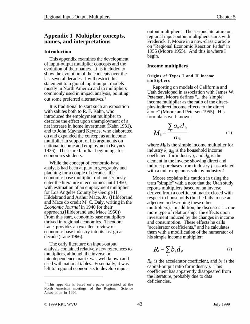
Regional Input-Output Multipliers Chapter 5
© 1999 RRI, WVU 43 July 1999
Appendix 1 Multiplier concepts,names, and interpretations
Introduction
This appendix examines the developmentof input-output multiplier concepts and theevolution of their names. It is included toshow the evolution of the concepts over thelast several decades. I will restrict thisstatement to regional input-output modelsmostly in North America and to multiplierscommonly used in impact analysis, pointingout some preferred alternatives.1
It is traditional to start such an expositionwith salutes both to R. F. Kahn, whointroduced the employment multiplier todescribe the effect upon unemployment of anet increase in home investment (Kahn 1931),and to John Maynard Keynes, who elaboratedon and expanded the concept as an incomemultiplier in support of his arguments onnational income and employment (Keynes1936). These are familiar beginnings foreconomics students.
While the concept of economic-baseanalysis had been at play in geography andplanning for a couple of decades, theeconomic-base multiplier did not seriouslyenter the literature in economics until 1950,with estimation of an employment multiplierfor Los Angeles County by George H.Hildebrand and Arthur Mace, Jr. (Hildebrandand Mace do credit M. C. Daly, writing in theEconomic Journal in 1940 for theirapproach.(Hildebrand and Mace 1950))From this start, economic-base multipliersthrived in regional economics. TheodoreLane provides an excellent review ofeconomic-base industry into its last greatdecade (Lane 1966).
The early literature on input-outputanalysis contained relatively few references tomultipliers, although the inverse orinterdependence matrix was well known andused with national tables. Essentially, it wasleft to regional economists to develop input-
1 This appendix is based on a paper presented at theNorth American meetings of the Regional ScienceAssociation in 1990.
output multipliers. The serious literature onregional input-output multipliers starts withFrederick T. Moore in a now-classic articleon "Regional Economic Reaction Paths" in1955 (Moore 1955). And this is where Ibegin.
Income multipliers
Origins of Types I and II incomemultipl iers
Reporting on models of California andUtah developed in association with James W.Petersen, Moore defines "... the 'simple'income multiplier as the ratio of the direct-plus-indirect income effects to the directalone" (Moore and Petersen 1955). Hisformula is well-known:
k
hj jkj
hk
Ma d
a=
∑(1)
where Mk is the simple income multiplier forindustry k, ahj is the household incomecoefficient for industry j, and djk is theelement in the inverse showing direct andindirect purchases from industry j associatedwith a unit exogenous sale by industry k.
Moore explains his caution in using theterm "simple" with a note that the Utah studyreports multipliers based on an inversederived from a coefficient matrix closed withrespect to households (but he fails to use anadjective in describing these othermultipliers). In addition, he discusses "... onemore type of relationship: the effects uponinvestment induced by the changes in incomeand consumption. These effects he calls"accelerator coefficients," and he calculatesthem with a modification of the numerator ofhis simple income multiplier:
k jj
jkR b d= ∑ (2)
Rk is the accelerator coefficient, and bj is thecapital-output ratio for industry j. Thiscoefficient has apparently disappeared fromthe literature, probably due to datadeficiencies.

Regional Input-Output Multipliers Chapter 5
© 1999 RRI, WVU 44 July 1999
Moore and Petersen report an interindustrymodel of Utah which remains a monument toscholarship. They go beyond Leontief'searlier-described "balanced regional model"(Leontief 1953) to develop a transactionstable with pure regional transactions, albeittransactions estimated with what Schaffer andChu later (1969) called the "supply-demandpool" technique, or the commodity-balanceapproach.
They proceed with development of threesets of income multipliers. Interestingly,especially given the problems we have facedover the years in terminology, they give thesemultipliers no specific names. The firstincome multiplier was the one named earlierby Moore as the "simple income multiplier."Its numerator was "income reactions tochanges in demand," or the direct and indirectincome effects of a unit change in finaldemand. The second was derived from"income reactions including induced viahomogeneous consumption functions," or thedirect, indirect, and induced income effects ofchange. The third multiplier was based on"income reactions including induced vianonhomogeneous consumption functions.This third multiplier was computed using themarginal coefficients in consumptionfunctions estimated from national data foronly three aggregations of the seven-industrymodel used to illustrate the study. Moore andPetersen felt that the induced effect isoverstated by the homogeneous consumptionfunctions implied by the closure of the modelwith respect to households.
Werner Z. Hirsch, in his model of St.Louis, moved beyond Moore and Petersen inthree ways: he built the model from companyrecords, he prepared a detailed exports matrix,and he treated the household and localgovernment sectors as endogenous parts ofthe economy (Hirsch 1959). But he remainedconsistent in his treatment of incomemultipliers, although he developed only twosets and gave them parenthetic names.Moore's simple income multiplier became"multiplier (Model I)" and his secondmultiplier became "multiplier (Model II)."
At this point, little attention had been paidto input-output multipliers in the literature. Inhis Methods of Regional Analysis, Walter
Isard, pays scant attention to them, sevenpages out of over 700, devoted almostexclusively to the income and employmentmultipliers of the Utah study (Isard 1960).Hollis B. Chenery and Paul G. Clark, in theirInterindustry Economics, long thecomprehensive reference in the field, cite theterm "multiplier" only twice in their index(Chenery and Clark 1959). Chenery andClark do build inverses for Model I andModel II tables, as did Hirsch, with the ModelII tables including households asendogenous.
But in 1965, William H. Miernyk devoted14 pages of over 150 to multiplier analysis,and 8 of these to income multipliers. Simple,clear, and easily understood, Miernyk'sElements of Input-Output Analysis (Miernyk1965) became a virtual bible to buddingregional input-output analysts. Interest inregional input-output studies was intensifyingin the sixties, and with this interest came aneed to present in study reports some of thetools which might help others in usingmodels produced at substantial expense andeffort.
Miernyk based his table illustrating"income interactions" on a similar table fromHirsch. But he changed column headingsdescribing multipliers for models I and II tobe "Type I multiplier" and "Type IImultiplier." To my knowledge, this is thebeginning of the line for these names, whichare still in use today. My suspicions areconfirmed by P. Smith and W. I. Morrison,who calculated income multipliers "... usingmethods developed by Hirsch and discussedfurther by Miernyk, ... described (afterMiernyk) as type 1 and type 2 incomemultipliers" (Smith and Morrison 1974, p.57).
Type III multipliers
Moore and Petersen as well as Hirschdeveloped crude consumption functions forsets of industries in an attempt to reduce theimpact of average propensities to consume (asexpressed in a household coefficientscolumn) on the induced income effectincluded in their type II multipliers. But theresulting third set of multipliers wasunnamed. Miernyk obliged in his Boulder

Regional Input-Output Multipliers Chapter 5
© 1999 RRI, WVU 45 July 1999
study by labeling these multipliers as "typeIII multipliers." Miernyk calculatedconsumption functions in Boulder andapplied estimated marginal propensities toconsume instead of household coefficients incomputing income multipliers. As heexpected, the resulting type III multiplierswere lower than type II multipliers by slightlymore than 10 percent. (Miernyk et al. 1967)
A second definition of type III multipliersis in use in Canada in the Atlantic Provincesand Nova Scotia (See Jordan and Polenske1988 for a clear summary.). Following thelead of Kari Levitt and a team at StatisticsCanada, I used three levels of closure todevelop output, income, and employmentmultipliers for the 1974, 1979, and 1984Nova Scotia input-output models (DPAGroup Inc. and Schaffer 1989). Model I isthe traditional open model, yielding direct andindirect effects; model II is closed withrespect to households, yielding direct, indirect,and induced effects; model III is closed withrespect to local and provincial governmentsectors as well, yielding direct, indirect, andextended effects. We devised the term"extended effects" to include effects inducedboth by households and by local andprovincial governments.
This treatment of type III multipliers asreflective of greater closure seems a better useof the numbering system.
Household-income multipliers
Income multipliers are the mosttroublesome of multipliers. When wedocumented the Hawaii input-output modelfor 1967 the problems became obvious(Schaffer et al. 1972). Because it was by thentraditional to show income and outputmultipliers, we did so, designating them as"simple" and "total," feeling these terms moredescriptive than "type I" and "type II." (The"simple" came from the income multiplier inMoore and Petersen; the "total" came fromtheir employment multiplier.) But we couldnot recall any instance in which theDepartment of Planning and EconomicDevelopment or any other agency had beenasked to show the total effect on householdincomes of a specified direct income changedue to exogenous forces on an industry.
People asked about the impact of new plantinvestment (a problem for which noconvenient multipliers have been constructed)and about the impact of export sales, but nonewould ask about the effect of a payrollincrease. So we added an "incomecoefficient," showing the total income effectassociated with a unit change in export sales.The format of the table was Hirsch's (1959, p.366), with a total column added.
In documenting the 1970 Georgia input-output model, (Schaffer 1976), the traditionaldefinition became "... awkward andinconsistent with the approach taken in mostinterpretations. Therefore, we ... defined the'household-income multiplier' for industry j tobe the addition to household incomes in theeconomy due to a one-unit increase in finaldemand for the output of industry j." Thefootnote explaining this move is a clearsummary of the twisted path described thusfar:
The notion of an income multiplier as firstintroduced to the regional literature by Moore andPetersen (1955) was used to describe additionalhousehold income attributable to unit change inhousehold income in the industry in question. Thisdefinition is far removed from the exogenouschanges which precipitate additional incomechanges, and it forces its user to unnecessarytrouble in determining, e.g., the importance of anindustry to its community. We have thereforeswitched ... . Although a similar concept appearedin Moore and Petersen, ... our point is that thelabel is confusing. We first saw this conceptdiscussed as 'income coefficients' in the Mississippistudy by Carden and Whittington (1964) and usedthe term to distinguish our multiplier from the oneseen in the literature as late as 1973. (p. 67)
Davis (1968, p. 33) makes the importance of thisdistinction clear. Two old-style income multipliersmay have exactly the same values but may differsubstantially in terms of income change per unitchange in final demand. He suggests that anemphasis on absolute changes ... rather than onrelative changes, as in Moore and Petersen, be madeto avoid the confusion. The caution was alsoexpressed by Miernyk (1967, p. 101) in his Boulderstudy, which reported old-style income multipliers.
But despite these problems, the old-styleincome multipliers live on. Two not-too-distant uses are in the Delaware modelproduced by Sharon Brucker and SteveHastings (1984) and in the 1984 Nova Scotia

Regional Input-Output Multipliers Chapter 5
© 1999 RRI, WVU 46 July 1999
Study, where the term 'income-generatedmultiplier' substitutes for the above-recommended 'household-income multiplier'and 'income multipliers' are defined in theoriginal way.
Other income multipliers
It became obvious early that othermultipliers reflecting the total impact ofchanges in final demand on incomes could begenerated.
The documentation of the 1963Washington input-output (Bourque andothers 1967) reports only one multiplier, theregional income multiplier, which includes thechange in total state income per $100,000change in final demand. The 1972Washington study (Bourque and Conway1977), in one of the clearest expositions ofmultiplier development yet written, definestype I and type II value added multipliers,along with labor-income multipliers, and jobsmultipliers. In each case, the multiplier iscalculated as "... a simple transformation ofthe output multipliers given in the inversematrix ... ." Thus:
k kj iji
kj ijM v b v b= ∑ ∑ (3)
where Mk is the income multiplier for the kthfactor income, vki is the input coefficient for
the kth factor in industry i, and bij is theinverse coefficient.
This view of the multiplier as an operatorwith which to transform changes in industryoutput into impacts on incomes of factors ofproduction was well expressed by Hays B.Gamble and David L. Raphael (1966). In asurvey-based model of Clinton County,Pennsylvania, they develop "residual incomemultipliers" by inverting a coefficient matrixincluding vectors for the nonprofit sector,three local government sectors, and fourhousehold sectors. Then by summingelements in these rows of the interdependencymatrix (inverse) for each industry, theyproduced household multipliers, localgovernment multipliers, and nonprofitmultipliers.
In both the Nova Scotia studies and theGeorgia model, I produce government-incomemultipliers. for local governments and forprovincial or state governments.
In all these cases, the multipliers can beunambiguously interpreted as changes inincomes per change in exogenous demand. Itis only the income multiplier associated withhouseholds that is ambiguous.
Employment multipliers
Employment multipliers were developed byMoore and Petersen at the same time as andanalogous to their income multipliers. Theyestimated a set of aggregated employment-production relationships and used thecoefficients showing change in employmentper change in output as the a's in equation (1),transforming the multiplier from dollar termsinto employment terms. Their multipliersrelate total employment change to directemployment change.
Both Hirsch and Miernyk repeat thisdefinition. In his Boulder study, Miernykbuilt "type III" employment multipliers aswell, with a complete set of employmentfunctions. Later, in his West Virginia Study,Miernyk apparently used simpleemployment-output ratios to effect thetransformation from output terms toemployment terms.
The first employment multipliers producedin the Washington series were for 1972.Bourque and Conway unwaveringly maintaintheir devotion to defining multipliersdenominated with final demand changes,producing type I and type II versions toreflect levels of closure.
In Georgia, I also denominated my simpleand total employment multipliers with finaldemand changes. In Nova Scotia, weproduced both output-based employmentmultipliers and employment-basedemployment multipliers for models with threelevels of closure, parallel to our othermultipliers. This was largely because of afeeling that, in inflationary times, the shelf lifeof output-based employment multipliers wasmuch lower than that of employment-basedones.

Regional Input-Output Multipliers Chapter 5
© 1999 RRI, WVU 47 July 1999
Output multipliers
Output multipliers are an obvious startingpoint for multiplier analyses. They aresimply the column sums of the industry partof an inverse matrix. These columns are theessential ingredients in the other multipliercalculations. Yet, output multipliers wereneither mentioned nor alluded to by eitherMoore and Petersen or Hirsch or Miernyk.
Floyd Harmston in his 1962 Wyomingstudy used a “business and industrymultiplier” which was a type I outputmultiplier under another name (Harmston1962). I used output multipliers in bothGeorgia and Nova Scotia studies. But, after alittle note from Rod Jensen, Australia’aleading authority on input-output analysis,commenting on an early draft, I made explicita warning that output multipliers should beused only as general indicators of industrialactivity. While they represent the essence ofinterindustry models, the flows ofintermediate transactions are not our basicinterests in summary multipliers. Effects onincome and employment are our primaryconcerns. Nevertheless, these by-products ofuseful multiplier production are commonstatements in many studies.
In explaining why they did not produceaggregate output multipliers for the 1972Washington model, Bourque and Conwayexpress this caution beautifully:
... we have not specified aggregate outputmultipliers. Although the output multipliers givenby the elements of the inverse matrix are at the rootof the multipliers ...[calculated] ... , it is not verymeaningful to sum these elements into aggregateoutput multipliers for each industry ... . In otherwords, given the concepts that lie behind eachoutput measure, it does not make much sense,economically speaking, to combine, say, theshipments of pulp mills with the margins of theinsurance industry into an aggregate transactionsmeasure. Furthermore, users of the Washingtontables in the past have sometimes employedaggregate output multipliers inappropriately, in atleast one case confusing them with incomemultipliers. For these reasons, we have chosen notto present aggregate output multipliers. (Bourqueand Conway 1977, p. 48)
Observations and summary
It is useful to conclude these commentswith a look at Table 5.4, reporting thesummary of general multiplier formulasprovided in the recent comprehensivecompendium on input-output analysis byRonald E. Miller and Peter G. Blair (1985).Multipliers have admittedly become a largerquestion than for earlier writers. Miller andBlair devote over ten percent of their book toregional, interregional, multiregional, andinterrelation multipliers. (Only five percent isdevoted to basic regional multipliers.)
They resolve my concern regarding thedenominating of income and employmentmultipliers by relegating the terms "type I"and "type II" exclusively to multipliers withdenominators in the same terms as thenumerators. They then use the terms"simple" and "total" to identify multipliersbased on pure industry transactions tablesand tables closed with respect to households.They specify multipliers based on finaldemand changes as "household" incomemultipliers, or "household" employmentmultipliers.
These statements and the explanationsaccompanying them are helpful indeed. But,an appropriate conclusion of this review isthat analytic purposes determine theterminology to use. The problem which wemight perceive comes from overall studyreports which suggest through terminologythe impacts which might be examined throughregional input-output models. Whenparticular questions are pursued, explanationsshould eliminate the ambiguities in impactinterpretations.
Further extensions
The point of view taken above can bedescribed as that of an old-line traditionalist.More multipliers continue to evolve andrecirculate. I should mention two of them
One is income-distribution multipliers. tomy knowledge, efforts to develop income-distribution multipliers started with RolandArtle in his studies of the Stockholmeconomy (Artle 1965) and in his efforts in theearly sixties to estimate such multipliers whileworking with a research team in Hawaii.

Regional Input-Output Multipliers Chapter 5
© 1999 RRI, WVU 48 July 1999
While he conceptualized a system with thehousehold row divided into several incomeclasses and with the household expenditurecolumn similarly divided, the effort failed dueto complex data problems.
An effort which has yielded more fruit isthat of Kenichi Mizyzawa documented inseveral articles in the sixties and seventies andin his book (Miyazawa 1976). His“intersectoral income multipliers” have beenused on numerous occasions in the last twodecades. Since such studies are beyond therealm of normal economic impact analyses,we do not treat them further.
The second multiplier system that has beenresurrected is the “SAM-based multiplier.”Social Accounting Matrices (SAMs) evolvedto a high level in the sixties in several streamsof literature. One is the work of Richard A.Stone (leading to his Nobel Laureate inEconomics) and extended at great detail in theUnited Nations social accounting literature.Another is the work at Statistics Canada asexemplified in the most exhaustive theoreticaland empirical analysis of social accounts byKari Levitt for the Atlantic Provinces (Levitt1975a; 1975b). A third outstanding exampleof social accounting was executed by the lateJerald R. Barnard at the University of Iowa(Barnard 1967).
Each of these streams resultedinterindustry studies augmented by socialaccounts documenting incomes in varioussectors of the economy (detailed income andproduct accounts of which the aggregatedregional accounting table in Chapter 3 is asimple example) and yielding multipliers forthe various sectors.
A more recent example of SAM multipliermodels is the one in current use by IMPLAN,the modeling system developed by MIG, Inc.(Minnesota IMPLAN Group Inc. 1997)
A final comment is simply a caution. Theproliferation of multipliers over the years andthe complexity of extensions to input-outputanalysis can lead to substantial confusionamong even knowledgeable analysts. Anymultiplier analysis intended for a broadaudience (or even an important decision-making audience) should be reduced to thesimplest possible terms but should be
sufficiently documented to permit someevaluation of its conclusions.

Regional Input-Output Multipliers Chapter 5
© 1999 RRI, WVU 49 July 1999
Table 5.4 Summary of multiplier names and formulas from Miller andBlair, Input-Output Analysis
MULTIPLIER ALGEBRAIC
CATEGORY DEFINITION
Output
Simple
Oj = α ij∑i=1
n
Total
Oj = α ij∑i=1
n+1
Income
Simple household
Hj = an+1, iα ij∑i=1
n
Total household
Hj = an+1, iα ij∑i=1
n+1
Type I
Yj = Hj/an+1, j
Type II
Yj = Hj/an+1, j
MULTIPLIER ALGEBRAIC
CATEGORY DEFINITION
Employment
Simple household
Ej = ∑i=1
n
Wn+1, iα i j
Total household
Ej = ∑i=1
n+1
Wn+1, iα i j
Type I
Wj = Ej/Wn+1, j
Type II
Wj = Ej/Wn+1, j

© 1999 RRI, WVU 50 Draft July 28, 1999
6 INTERREGIONAL MODELS
Now we can easily combine the economic-base and interindustry concepts to yield aquick feeling for multi-regional models.While we stop with this introduction,extensions to include transactions betweenindustries in different regions are immediatelyobvious. In fact, a considerable literature hasdeveloped on interregional interindustrymodels and efforts have even been made torelate such models to “other worlds” such asthe environment delineating the interactions ofthe human economy with the highlyinteractive elements of our land, sea, and air“economies.”
Interregional economic-base modelsIn the following summary models, I have
left implicit the definitions and identitieswhich we labored over before. The commonglossary is as follows:
Y: incomeE: income-related expendituresEi: income-related expenditures in region iEij: income-related expenditures in region i
by residents of region jA autonomous expenditurese: marginal propensity to spend,
dE(Y)/dY=eX: exportsM: importsm: marginal propensity to import,
dM(Y)/dY=m
i: subscript for region (A subscript of 0 isfor “autonomous value.” )
Review of one-region models
The one-region models are the Keynesianand economic-base models. Theirdistinguishing characteristic is that the valueof income is determined by someautonomous activity out there. It may beinvestor behavior, as in the Keynesian model,
or it may be purchases by consumers outsidethe region, as in the economic-base model.
Closed economy, no external trade
Assumptions:
E = E(Y) = eY
A = A0
Equilibrium condition:
Y = E + A
Solution:
Y = eY + A0
Y = [1/(1 - e)] A0
Multiplier:
dY/dA = 1/(1-e)
Open economy, with trade leakage
Assumptions:
E1 = E1(Y1) = e1Y1
X1 = X0
M1 = M1(Y1) = m1Y1
A1 = A0
Equilibrium condition:
Y1 = E1 + A1 + X1 - M1
Solution:
Y1 = e1Y1 + A0 + X0 - m1Y1
Y1 = (A0 + X0)* 1/(1 - (e1 - m1))
Multiplier:
dY1/dX0 = dY1/dA0 = 1/(1-(e1 - m1))
Two-region model with interregionaltrade
What has been missing all along has beeninteraction between regions. Obviously thistakes place in the real world; otherwise, therewould be no regions. Exports by one regionhave to be imports into another economy.

Interregional Models Chapter 6
© 1999 RRI, WVU 51 Draft July 28, 1999
Partial solution, two-region interregionalmodel
The system can more easily be presentedby laying out the system in the same form asabove but stopping before the algebrarequires the theory of determinants, which haseither been forgotten or ignored by most ofus. We will limit the statement to region onealone in this section.
Assumptions:
E1 = E1(Y1) = e1Y1
X1 = M2 = M2(Y2) = m2Y2
M1 = M1(Y1) = m1Y1
A1 = A0
Equilibrium condition:
Y1 = E1 + X1 - M1 + A1
Solution:
Y1 = e1Y1 - m1Y1 + m2Y2 + A0
dY1 = e1dY 1- m1dY 1 + m2(dY2/dY1) dY1 +dA0
dY1 = e1dY 1- m1dY 1 +m2(dY2/dY1)dY1(dM1/dX2) + dA0
dY1 = e1dY 1- m1dY 1 + m2 m1 (dY2/dX2) dY1+ dA0
But this line of attack becomes unnecessarilycomplicated. We can't easily reduce theinteractive term without knowing themultiplier for the other region (dY2/dX2)!
Multiplier:
dY1/d A0 = 1/(1-(e1 - m1 +m2 m1 (dY2/dX2))
dY1/d A0 = 1/(1-(e1 - m1 + interregionaleffect))
Let us take a more familiar tack. (Thisapproach originated with Alan Metzler(Metzler 1950); Harry Richardson providesthe restatement on which the above is based(Richardson 1969)
Matrix solution, two-region interregionalmodel
This model can be more systematicallyexpressed with the matrix algebra developedfor input-output analysis. Matrix algebrapermits us to immediately extend our logicfrom two regions as above to n regions
without producing page after page ofcumbersome calculations. Nevertheless, wewill work with a two-region system forsimplicity of discussion. We proceed asfollows:
Assumptions:
As above, but now for both regions 1 and 2.
Ei = Ei(Yi) = eiYi
Xi = Mj = Mj(Y j) = mjYj
Equilibrium conditions:
E1 + X1 - M1 + A1 = Y1
E2 + X2 - M2 + A2 = Y2
Rewrite to align purchases from the tworegions:
E1 - M1 + X1 + A1 = Y1
X2 + E2 - M2 + A2 = Y2
Now, observing the following definitions, wecan rewrite the equation system preparatory tomatrix manipulation:
E11 = E1 - M1 = e1Y1 - m1Y1 = e11Y1
E12 = M2 = M2(Y2) = m2Y2 = e12Y2
E21 = X2 = M1(Y1) = m1Y1 = e21Y1
E22 = E2 - M2 = e2Y2 - m2Y2 = e22Y2
Note that the e's now show double subscriptsshowing purchases from region i by region j.So the system becomes
E11 + E12 + A1 = Y1
E21 + E22 + A2 = Y2
or
e11Y1 + e12Y2 + A1 = Y1
e21Y1 + e22Y2 + A2 = Y2
which translates into matrices as
e11 e12 Y2 + A1 = Y1 e21 e22 Y2 + A2 = Y2or
eY + A = Y
where e is the matrix of eij. This solvesexactly as would an input-output system:
Y - eY = A

Interregional Models Chapter 6
© 1999 RRI, WVU 52 Draft July 28, 1999
(I - e)Y = A
(I - e)-1(I - e)Y = (I - e) -1A
Y = (I - e) -1A
Now, to give the elements of this inverse adesignation, set
R = (I - e)-1 = R11 R12 R21 R22rewrite the solution as
Y1 = R11A1 + R12A2
Y2 = R21A1 + R22A2
The interregional multipliers are thus
dYi/dAj = Rij
for each ith row and jth column.
Now, it is a simple matter to expand thesystem to treat n regions. The process isidentical to that used in the two-region systembut with larger matrices!
Extensions and further study
Interregional interindustry models
The obvious extension is to expand the cellentries to become interindustry transactionsmatrices. Thus the E12 entries would becomeklEij, showing purchases from industry k inregion i by industry l in region j; where i=j ,the regional transactions matrix for region i isinserted, and where i is not equal j, a matrixof imports is inserted.
The most commonly used multi-regionalinterindustry model of the United States wasassembled by Professor Karen Polenske atMIT. Her model includes transactionsgenerally for 50 industries in each of 44states or sets of states.(Polenske 1980)
Economic-ecologic models
Economic-ecologic models appendmatrices depicting interaction between sectorsin the natural environment and between thosesectors and the industrial ones. The conceptis similar to interregional interindustryanalysis but implementation becomes aharrowing experience. The dominantexample of this was a complex model of theMassachusetts Bay area. (Isard et al. 1972)
Both of these extensions are discussed indetail in the comprehensive input-outputreference by Ronald Miller and Peter Blair.(Miller and Blair 1985)
Study questions1. Outline a simple two-region interregional model,
convert it to matrix form, and solve the system.
2. Construct the model for a closed economy withno external leakage in matrix form as in question(1). Identify elements in the multiplier matrix.
3. Construct the model for an open economy withtrade leakage but no interregional linkage inmatrix form as in question (1). Identify elementsin the multiplier matrix.
4. Compare the multipliers for (say region 1) in aninterregional economy, a closed economy, and anopen economy with trade leakage. Which systemhas the largest multipliers? Which the smallest?

© 1999 RRI, WVU 53 Draft July 28, 1999
7 COMMODITY-BY-INDUSTRY ECONOMICACCOUNTS: THE NOVA SCOTIA INPUT-OUTPUT
TABLES
IntroductionNow that we have the basic framework of
input-output analysis in hand, let's move alittle closer to the format in which data is nowaccumulated at the national level and fromwhich we estimate the parameters of regionalmodels.
This format was developed in the 1960s byRichard A. Stone at Cambridge and adoptedas a standard by the United Nations. Stonelater received the Nobel Prize in Economicsfor his work in national income accounting(which includes input-output accounting).Statistics Canada (the statistical agency inCanada) pioneered in applying this formatstarting with their 1960 table; the Input-Output Division of the U.S. Department ofCommerce produced their 1972 table in thenew format. As a result, most of the state andregional models produced today are based onthis format and data source.
This format is called the "commodity-by-industry" format, and sometimes the"rectangular" system. It is rectangular in thatthe commodity dimension may be greaterthan the industry dimension (which poses aproblem when the direct-requirements matrixmust be square to provide a solvable system).It originated with a realization that firms,grouped in industries, buy commodities andthat we have trouble grouping commoditiesinto industries. Firms often produce severalcommodities. They are classified intoindustries according to their primaryproducts; their remaining products aresecondary. An accounting scheme has tomanage this problem.
I had the pleasure of building three input-output systems in Nova Scotia (1974, 1979,and 1984) during the period when thecomputing world moved from mainframes todesktops. The system fits exactly with thenew U.S. system. Chapters 8 and 9 parallelChapters 4 and 5 in organization and content.
My intention is to make the transition to themore complex modern system easier as wellas to economize on the writing chore.(DPAGroup Inc. and Schaffer 1989)
The Nova Scotia input-output tablesrepresent a complete set of social accounts forthe Province. As is common with most socialaccounts, it is double entry in nature, but ithas been organized in matrix form rather thanas the traditional T-accounts. This sectionpresents a brief schematic review of theaccounting framework. In addition, theinterpretation of the Nova Scotia tables isdemonstrated with a set of highly aggregated(five-industries) tables which duplicate theformat of the more detailed tables produced inthe Nova Scotia Input-Output Study itself.
A schematic social-accountingframework
The Nova Scotia input-output tables followthe form of the Canadian tables. They are ofthe "rectangular form" and show substantiallymore of the commodity detail of industrypurchases than do tables of the "square" formcommonly used in the United States andelsewhere. As shown in Illustration 7.1, thetables comprise six matrices. Three sets ofaccounts are evident in these matrices and thecomments which follow are intended toidentify the accounts in the tables.
Commodity accounts
For each commodity used and/or producedin the Province, accounts representing supplyand demand can be constructed. Thus, theshaded row in Illustration 7.2 presents thedemand side of the supply-and-demandequation for a particular commodity. It

Commodity-by Industry-Economic Accounts Chapter 7
© 1999 RRI, WVU 54 Draft July 28, 1999
Illustration 7.1 Schematic input-output table for Nova Scotia
TOTA
L CO
MM
ODI
TY D
EMAN
D
TOTAL FINALOUTLAYS
TOTAL INDUSTRYINPUTS
VECTOR 6:COMMODITY IMPORTS M
m1 2 3 . . .
COMMODITIES
1
2
3
.
.
.COM
MO
DITI
ES
MATRIX 5
COMMODITY ORIGINS
OR INDUSTRY OUTPUTS
MATRIX 3
FACTOR USES
MATRIX 4
NONMARKET
TRANSFERS
PRIM
ARY
INPU
TSE
CTOR
S
1
2
3
n
. .
H
C
G
.
.
.
TOTA
L IN
DUST
RYO
UTPU
TS
SUM TOTAL COMMODITYSUPPLY
SUM
PROD
UCIN
GIN
DUST
RIES
USING INDUSTRIES SECTORSCONSUMING
MATRIX 2 MATRIX 1
COMMODITY FINALUSES OR DEMANDS
INDUSTRY BY INPUTS CONSUMERS
TOTA
L FA
CTO
RRE
CEIP
TS
.
1 2 3 . . . n H C G . . . E

Commodity-by Industry-Economic Accounts Chapter 7
© 1999 RRI, WVU 55 Draft July 28, 1999
Illustration 7.2 Schematic input-output table for Nova Scotia emphasizingthe commodity accounts
TOTA
L C
OM
MO
DIT
Y D
EMAN
DTOTAL FINAL
OUTLAYSTOTAL INDUSTRY
INPUTS
VECTOR 6:COMMODITY IMPORTS M
m1 2 3 . . .
COMMODITIES
1
2
3
.
.
.CO
MM
OD
ITIE
S
MATRIX 5
COMMODITY ORIGINS OR
INDUSTRY OUTPUTS
MATRIX 3
FACTOR USES
MATRIX 4
NONMARKETTRANSFERS
PRIM
ARY
INPU
TSE
CTO
RS
1
2
3
n
.
.
C
G
.
.
.
.SUM TOTAL COMMODITYSUPPLY
SUM
PRO
DUCI
NGIN
DU
STR
IES
USING INDUSTRIES SECTORSCONSUMING
MATRIX 2 MATRIX 1
COMMODITY FINALUSES OR DEMANDS
INDUSTRY BY INPUTS CONSUMERS
TOTA
L FA
CTO
RRE
CEIP
TSTO
TAL
IND
UST
RY
OU
TPU
TS
H
1 2 3 . . . n H C G . . . E
.

Commodity-by Industry-Economic Accounts Chapter 7
© 1999 RRI, WVU 56 Draft July 28, 1999
shows both the intermediate uses, ordemands, expressed by domestic industriesfor the commodity, as recorded in Matrix 2,and the final uses, or demands, by consumingsectors for the commodity, as recorded inMatrix 1. These consuming sectors includelocal consumers and investors, governments,and non-local users. Total demand is the sumof total industry demand and total finaldemand.
The supply side of the equation for acommodity is represented in Illustration 7.2by the shaded column, which traverses Matrix5 and Vector 6. In Matrix 5, this columnidentifies the domestic industrial origins ofthe commodity; Vector 6 identifies imports ofthe commodity. The column sum is totalsupply, which is equal to total demand.
Industry accounts
The inputs and outputs of industries canalso be traced in this system. Illustration 7.3moves the shaded column and row torepresent inputs and outputs of a particularindustry. The outputs of the industry can beseen in the shaded row. This row records thevalues of the various commodities producedby the industry. The column in Illustration7.3 records the production technology of theindustry in terms of commodities purchasedin Matrix 2 and of payments to "primary"inputs (i.e., labor, return to capital, etc.), orfactors of production, in Matrix 3. Since thepayments to inputs include profits, or theresidual receipts by owners of establishmentsin the industry, total inputs equal total outputsfor the industry.
Final accounts
The incomes and expenditures of"primary" sectors (e.g. household,government, etc.) of the economy can also betraced through the system. The shaded rowand column in Illustration 7.4 are illustrative.The shaded row represents the incomes of a"primary" sector such as households or agovernment. As seen in Matrix 3, theseincomes are paid by industries which use theservices of the factors of production owned orprovided by the sector. In addition, transfersof incomes from other "primary" sectors arerecorded in Matrix 4. With the exception of
wages and salaries paid by households,governments, and outside employers these"transfers" are non-market in nature andrepresent such items as taxes, savings, welfarepayments, intergovernmental transfers, andsurpluses and deficits.
In accounting for gross provincial product,the row sums of Matrix 3 represent incomesof domestic factors as paid by the private, orindustrial, sectors of the economy. Theaddition of incomes earned by householdsfrom the primary sectors in Matrix 4completes the income side of gross provincialproduct. This tabulation of incomesrepresents value added in the economy.
The shaded column in Illustration 7.4represents the final expenditures by aprimary-input sector. In Matrix 1, thecommodity detail of such expenditures isshown, and in Matrix 4, the transfers(including wages and salaries) to otherprimary sectors are recorded. The sum ofthese commodity purchases and transfers istotal expenditures, which is equal to totalreceipts by the sectors.
The expenditures side of the grossprovincial product account consists of thesum of total purchases of goods and servicesby domestic primary sectors, householdincomes received from these sectors, andgross commodity exports less industryimports (or net exports).
Aggregated input-output tablesWith this overall scheme in mind, consider
now the format of the actual tables. Small,highly aggregated (5-industry) versions of thetables are used as illustrations.

Commodity-by Industry-Economic Accounts Chapter 7
© 1999 RRI, WVU 57 Draft July 28, 1999
Illustration 7.3 Schematic input-output table for Nova Scotia emphasizingthe industry accounts
TOTA
L C
OM
MO
DIT
Y D
EM
AN
D
TOTAL FINALOUTLAYS
TOTAL INDUSTRYINPUTS
VECTOR 6:COMMODITY IMPORTS M
m1 2 3 . . .
COMMODITIES
1
2
3
.
.
.CO
MM
OD
ITIE
S
MATRIX 5
COMMODITY ORIGINS
OR
INDUSTRY OUTPUTS
MATRIX 3
FACTOR USES
MATRIX 4
NONMARKET
TRANSFERS
PR
IMA
RY
INP
UT
SEC
TOR
S
1
2
3
n
. . .
H
C
G
.
.
.TO
TAL
IND
US
TRY
OU
TPU
TS
SUM TOTAL COMMODITYSUPPLY
SUM
PRO
DU
CIN
GIN
DU
STR
IES
USING INDUSTRIES SECTORSCONSUMING
MATRIX 2 MATRIX 1
COMMODITY FINAL
USES OR DEMANDS
INDUSTRY BY
INPUTS CONSUMERS
TOTA
L FA
CTO
RR
EC
EIP
TS
1 2 3 . . . n H C G . . . E

Commodity-by Industry-Economic Accounts Chapter 7
© 1999 RRI, WVU 58 Draft July 28, 1999
Illustration 7.4 Schematic input-output table for Nova Scotia emphasizingthe final Income and expenditure accounts
RECEIPTS
TOTA
L C
OM
MO
DIT
Y D
EM
AN
D
TOTAL FINALOUTLAYS
TOTAL INDUSTRYINPUTS
VECTOR 6:COMMODITY IMPORTS M
m1 2 3 . . .
COMMODITIES
1
2
3
.
.
.CO
MM
OD
ITIE
S
MATRIX 5
COMMODITY ORIGINS
OR INDUSTRY OUTPUTS
MATRIX 3
FACTOR USES
MATRIX 4
NONMARKET
TRANSFERS
PR
IMA
RY
INP
UT
SEC
TOR
S
1
2
3
n
. . .
H
C
G
.
.
TOTA
L IN
DU
STR
YO
UTP
UTS
SUM TOTAL COMMODITYSUPPLY
SUM
PRO
DU
CIN
GIN
DU
STR
IES
USING INDUSTRIES SECTORSCONSUMING
MATRIX 2 MATRIX 1
COMMODITY FINAL
USES OR DEMANDS INDUSTRY BY
INPUTS CONSUMERS
TOTA
L FA
CTO
RR
ECEI
PTS
1 2 3 . . . n H C G . . . E
.

Commodity-by Industry-Economic Accounts Chapter 7
© 1999 RRI, WVU 59 Draft July 28, 1999
The commodity flows table
The commodity flows table combines theuse, final demand, and associated incomematrices (Matrices 1, 2, 3 and 4) ofIllustration 7.1. (In the national tables, thetwo equivalent tables are described as the "usematrix" (example Matrices 2 and 3) and the"final demand matrix" (example Matrices 1and 4). Table 7.1 is the aggregatedcommodity flows table. The boundariesbetween the various matrices are marked by arow for total commodity inputs and a columnfor total industry demands. This table is acomplete description of commodity purchasesby all Nova Scotia industries, all domestic andgovernment consumers, and all non-localpurchasers.
Note that the commodity flows table doesnot distinguish between commoditiesproduced domestically and those importedfrom outside the Province. The table whichembodies this distinction is called the"provincial flows table" and is presented inthe next chapter as the first stage indeveloping the input-output model.
The commodity origins table
The commodity origins table combines thedomestic origin matrix (5) and the importsvector (6) of Illustration 7.1 (In the nationaltables, the equivalent table is called the "makematrix"). Table 7.2 is an aggregatedcommodity origins table for Nova Scotiawhich is consistent with the aggregated flowstable.
Note that the origins table records morethan just the origins of commodities. It alsoincludes a complete tabulation of supply anddemand for each commodity used in NovaScotia. The last seven columns of the tablesummarize the commodity accounts of theProvince. The demands recorded here are thesame as the demand totals found in Table 7.1.Also note that the industry accounts arerepresented by the column totals found inboth tables. Total industry inputs are in Table7.1 while total industry outputs are in Table7.2.
For ease of production and in reading,columns represent industries and rowsrepresent commodities. This convention
requires that the domestic origins matrix andthe imports vector be transposed from theiroriginal form in Illustration 7.1.
Study questions1. Why were commodity-by-industry accounts
developed?

Commodity-by Industry-Economic Accounts Chapter 7
© 1999 RRI, WVU 60 Draft July 28, 1999
Table 7.1 Aggregated commodity flows, Nova Scotia, 1984
Extrac- Manufac- Con- Dis- Ser - Totaltion turing s t ruc- t r ibu- vice industry
Commodity ind. ind. tion tion ind. demand
1 Agricultural products 8 7 318 4 2 2 1 6 4472 Primary fish 3 179 0 0 1 1833 Minerals 6 1210 1 4 0 149 13794 Nondurable manuf. goods 154 648 8 6 8 5 737 17115 Durable manuf. goods 9 3 489 409 2 4 337 13526 Repair construction 1 0 2 5 1 7 225 2687 Residential construction 0 0 0 0 0 08 Nonresidential const. 0 0 0 0 0 09 Transp., comm. and util. 8 0 160 1 1 106 735 1092
1 0 Distribution 3 6 117 8 1 2 0 182 4361 1 Services 640 443 173 341 1109 2705
1 2 Total commodity inputs 1109 3589 779 604 3491 9573
1 3 Household receipts 535 899 391 877 2833 55351 4 Local and prov. govt rev 2 3 164 6 2 4 1 278 5681 5 Capital residual 9 2 136 5 2 137 704 11201 6 Federal govt revenues 0 - 1 0 2 9 2 3 6 2 1041 7 External transfers - 1 0 6 - 7 9 109 151 - 7 5 - 1
1 8 Total primary inputs 545 1109 641 1230 3802 7327
1 9 Total inputs 1654 4699 1420 1834 7293 16900
House- Local and Capi- Federal Domestic Totalhold prov. tal for- govt final Total final Total
Commodity exp. govt exp. mation exp. demand exports demand demand
1 Agricultural products 115 5 0 1 121 7 9 200 6462 Primary fish 2 0 0 0 2 8 4 8 5 2683 Minerals 2 1 7 696 0 716 133 848 22274 Nondurable manuf. goods 1679 139 147 6 0 2025 1639 3664 53745 Durable manuf. goods 810 1 8 611 114 1553 972 2525 38776 Repair construction 4 2 5 0 3 3 6 3 3 3 9 5 3637 Residential construction 0 0 541 0 541 0 541 5418 Nonresidential const. 0 0 600 1 1 610 4 0 651 6519 Transp., comm. and util. 523 194 0 8 4 802 203 1005 2097
1 0 Distribution 1174 2 8 112 1 0 1324 0 1324 17601 1 Services 2874 560 121 524 4079 4 9 4128 6833
1 2 Total commodity inputs 7182 987 2828 838 11835 3231 15066 24639
1 3 Household receipts 302 1839 0 2630 4771 2 2 4793 103281 4 Local and prov. govt rev 921 1804 6 6 1230 4021 1 4 4035 46031 5 Capital residual 418 141 0 0 559 0 559 16791 6 Federal govt revenues 1499 1 2 - 5 8 2 1248 2177 1 0 2187 22911 7 External transfers 1 7 0 0 0 1 7 0 1 7 1 6
1 8 Total primary inputs 3157 3796 - 5 1 6 5108 11545 4 6 11591 18918
1 9 Total inputs 10339 4783 2312 5946 23380 3277 26657 43557

Commodity-by Industry-Economic Accounts Chapter 7
© 1999 RRI, WVU 61 Draft July 28, 1999
Table 7.2 Aggregated commodity origins, Nova Scotia, 1984
Extrac- Manufac- Con- Dis- Ser - Totaltion turing s t ruc- t r ibu- vice industry
Commodity ind. ind. tion tion ind. supply
1 Agricultural products 353 2 0 0 0 3552 Primary fish 267 1 0 0 0 2683 Minerals 1032 1 0 0 0 10334 Nondurable manuf. goods 1 3324 0 6 0 33315 Durable manuf. goods 1 1367 0 4 3 3 14046 Repair construction 0 0 363 0 0 3637 Residential construction 0 0 406 0 0 4068 Nonresidential const. 0 0 651 0 0 6519 Transp., comm. and util. 0 0 0 0 1980 1980
1 0 Distribution 0 1 0 1598 1 3 16121 1 Services 1 3 0 226 5268 5498
1 2 Total inputs 1654 4699 1420 1834 7293 16900
Total Total dom-Total Total industry estic final Total Total
Commodity imports supply demand demand exports demand
1 Agricultural products 291 646 447 121 7 9 6462 Primary fish 0 268 183 2 8 4 2683 Minerals 1194 2227 1379 716 133 22274 Nondurable manuf. goods 2044 5374 1711 2025 1639 53745 Durable manuf. goods 2474 3877 1352 1553 972 38776 Repair construction 0 363 268 6 3 3 3 3637 Residential construction 135 541 0 541 0 5418 Nonresidential const. 0 651 0 610 4 0 6519 Transp., comm. and util. 117 2097 1092 802 203 2097
1 0 Distribution 149 1760 436 1324 0 17601 1 Services 1335 6833 2705 4079 4 9 6833
1 2 Total inputs 7739 24639 9573 11835 3231 24639

© 1999 RRI, WVU 62 Draft July 28, 1999
8 COMMODITY-BY-INDUSTRY INTERINDUSTRYMODELS: THE LOGIC OF THE NOVA SCOTIA INPUT-
OUTPUT MODEL
IntroductionThis section develops an economic model
from the accounting tables for Nova Scotia.The process parallels that used in thetraditional regional format presented inChapter 4. It differs in that we now shiftfrom a world in which regional economistscollect their own data into one requiring vastteams of statisticians. As seen in the previouschapter, much new information and detail isnow available. We need more assumptions toreduce it to a manageable format.
As the literature associated with theCanadian and Atlantic Provinces input-outputstudies suggests, and as demonstrated in theappendix to this chapter describing themathematics of the U.S. system, the modelcould be phrased in terms of commodities.The procedures are similar, however, and thereader is referred to the earlier literature forfurther details. Here we do a simple sketch.
Essentially, we manipulate the new systemof accounts until the number of variables in aset of simultaneous equations describing theeconomy equals the number of equations.The system differs slightly from thetraditional square regional matrices in thatnow we have not only more commodities (andso more equations) than industries but alsotwo equation systems to face! We mustdevise some way to redress this imbalance.
While the commodity-by-industry formattraditional to the Canadian and Nova Scotiainput-output systems opens up a variety ofpossibilities for forming this model, theapproach employed here develops a solutionto the model in terms of industries rather thancommodities. This means that, while theeconomy is described initially in terms of setsof equations representing the tables ofcommodity-by-industry flows and origins, wemust convert them to regional flows (throughapplication of the constant-importsassumption) and then reduce the equations to
a solvable form in industry-by-industrydimensions on the basis of the fixed market-share assumption. Finally, using theconstant-technology assumption, we can solvethe system conventionally.
The dataWe start with two sets of tables defining
the economy: The commodity flows tableand the commodity origins table. Both aredescribed in the previous chapter and are thesources for the use and make matrices usedbelow.
Technical conditionsNow say that final demands have been
estimated for some future date and that wewish to identify the effect of this demand onthe Province. What are the gross outputs ofindustries in Nova Scotia at that time? It isobvious that the system of flow equations isnot prepared for solution: in the flows table,there are 11 equations, one for eachcommodity, and 82 variables of which only11, the final demands, have preassignedvalues. Neither is the system of origins, ormake equations, which consists of 5equations and 66 unknowns.
The minimum requirement for solution ofthis system is that the number of equationsequals the number of unknowns. One task,therefore, is to reduce the number ofunknowns. Further, the system is expressedin terms of both commodity outputs andindustry inputs, while our stated goal is todetermine the effect of final-demand changeson industries. So a second task is to expressthe system in terms of industry variablesalone. This conversion will both reduce thenumber of equations and, more importantly,permit us to establish a familiar equilibriumcondition. The third and final task beforesolution is that of reducing the flows matrixfrom a statement of production technology to

Commodity-by Industry Economic Models Chapter 8
© 1999 RRI, WVU 63 Draft July 28, 1999
one of regional trade. We proceed in reverseorder.
The constant-imports assumption
Few of the recent regional input-outputstudies in this format have included survey-based, cell-specific import details. As a result,regional (or provincial, in this case) tradeflows must be estimated by assumption. Weknow imports for each commodity in thesystem (Table 7.2) and we know totalindustry domestic final demands. And that isall, so the best way to estimate regional tradeis to assume that each industry purchasesimported commodities in constantproportions:
µk = mk/(Σjukj + ek) (8-1)
where µk is the import coefficient forcommodity k , mk is an element in m, theimports vector, and the denominator is thesum of intermediate and local-final demandsfor commodity k.
Provincial flows of commodity k can thusbe estimated as
Pkj = ukj*(1 - µk) (8-2)
where uij is the purchase of commodity k byindustry j . This yields a set of equations forsales of locally produced commodities suchas the following:
P11 + P12 + ... + P1m + e1 + x1 = q1 (8-3)
P21 + P22 + ... + P2m + e2 + x2 = q2
. . ... . . . .
. . ... . . . .
. . ... . . . .
Pn1 + Pn2 + ... + Pnm + en + xn = qn
where Pkj is local sales of commodity k toindustry j, ek is sales of commodity k to finaldemand, xk is export sales of commodity k, qkis total local production of the commodity,and n and m are the number of commoditiesand industries, respectively. In this example,n is 11 and m is 5.
The results of this process are reported inTable 8.1, the aggregated provincial flows
table, showing purchases of commoditiesproduced by local industries. Note that it isvery similar to Table 7.1, the commodityflows table. It differs in the values ofcommodity purchases, which are now onlylocal in origin. It also contains a row ofimports (the external transfers row). Theindustry outputs and final demands remainthe same.
(Note here that imports were estimated atthe detailed, 602-commodity, worksheet levelusing uniform import coefficients for eachcommodity. These detailed worksheetspermit a level of realism not attainable whenestimates of imports are made at anaggregated level.)
The constant market-share assumption
The matrix reported in the commodityorigins table (Table 7.2) provides datanecessary for converting from a commoditysales dimension to an industry one. If eachentry (vjk) in the make matrix is divided by theappropriate total commodity output, theresulting coefficients can be used as weightswith which to aggregate commodity rows inthe provincial flows matrix. Called "domesticmarket-share coefficients", these weights arecomputed as
djk = vjk/ qk (8-4)
where djk is the market share of commodity kproduced by industry j, and qk is the totaldomestic output of commodity k . Thedomestic market-share matrix, D, iscomprised of these djk.
Now, assuming that market shares remainconstant, the provincial flows matrix P and thevector h representing local final demand canbe aggregated to industry-by-industrydimensions by matrix multiplication:
Z = D*P (8-5)
h = D*(e + x) (8-6)
This process means that each element zij in Zis a sum of weighted commodity sales,
zij = Σk (dik*Pkj ) (8-7)
and that sales are in proportion to the industryproduct mixes. The provincial final-demand

Commodity-by Industry Economic Models Chapter 8
© 1999 RRI, WVU 64 Draft July 28, 1999
Table 8.1 Aggregated commodity-by-industry provincial flows, Nova Scotia,1984
Extrac- Manufac- Con- Dis- Ser - Totaltion turing s t ruc- t r ibu- vice industry
Commodity ind. ind. tion tion ind. demand
1 Agricultural products 9 184 2 8 8 2102 Primary fish 3 179 0 0 1 1833 Minerals 4 2 0 1 2 0 148 1854 Nondurable manuf. goods 113 195 4 2 4 7 350 7465 Durable manuf. goods 2 2 9 3 118 8 5 0 2916 Repair construction 1 0 2 5 1 7 225 2687 Residential construction 0 0 0 0 0 08 Nonresidential const. 0 0 0 0 0 09 Transp., comm. and util. 7 6 155 1 1 9 5 689 1026
1 0 Distribution 3 3 5 8 7 5 1 7 168 3511 1 Services 122 398 110 288 826 1744
1 2 Total commodity inputs 392 1307 370 471 2464 50041 3 Household receipts 535 899 391 877 2833 55351 4 Local and prov. govt rev. 2 3 164 6 2 4 1 278 568
1 5 Capital residual 9 2 136 5 2 137 704 11201 6 Federal govt revenues 0 - 1 0 2 9 2 3 6 2 1041 7 Imports and transfers 612 2203 517 285 952 4568
1 8 Total primary inputs 1262 3391 1050 1363 4829 118961 9 Total inputs 1654 4699 1420 1834 7293 16900
House- Local and Capi- Federal Domestic Totalhold prov. tal for- govt final Total final Total
Commodity exp. govt exp. mation exp. demand exports demand demand1 Agricultural products 6 2 3 0 0 6 6 7 9 145 3552 Primary fish 2 0 0 0 2 8 4 8 5 2683 Minerals 2 1 7 696 0 715 133 848 10334 Nondurable manuf. goods 678 8 9 145 3 5 946 1639 2585 33315 Durable manuf. goods 4 1 3 8 0 1 7 140 972 1113 14046 Repair construction 4 2 5 0 3 3 6 3 3 3 9 5 3637 Residential construction 0 0 406 0 406 0 406 406
8 Nonresidential const. 0 0 600 1 1 610 4 0 651 6519 Transp., comm. and util. 496 176 0 7 9 751 203 954 1980
1 0 Distribution 1122 2 7 103 1 0 1261 0 1261 16121 1 Services 2705 445 119 436 3705 4 9 3754 54981 2 Total commodity inputs 5112 785 2149 620 8665 3231 11896 169001 3 Household receipts 302 1839 0 2630 4771 2 2 4793 103281 4 Local and prov. govt rev. 921 1804 6 6 1230 4021 1 4 4035 46031 5 Capital residual 418 141 0 0 559 0 559 16791 6 Federal govt revenues 1499 1 2 - 5 8 2 1248 2177 1 0 2187 22911 7 Imports and transfers 2087 202 679 218 3187 -7755 -4568 01 8 Total primary inputs 5227 3998 163 5326 14715 -7709 7006 189021 9 Total inputs 10339 4783 2312 5946 23380 -4478 18902 35801

Commodity-by Industry Economic Models Chapter 8
© 1999 RRI, WVU 65 Draft July 28, 1999
matrix, presented as the summed vector e andthe commodity exports vector x may besimilarly aggregated, yielding the vector h.
Table 8.2 reports domestic market-sharecoefficients as computed from the aggregatedmake matrix. That the transpose of this tabletimes the provincial flows matrices yieldsTable 8.3, the provincial interindustrymatrices, may be verified through applicationof equation 8-7.
This process has yielded an industry-by-industry provincial flows table and hasprepared the system for solution in terms ofindustry outputs. But the number of variableswith unknown values, 30, is still in excess ofthe number of equations, 5. The equationsystem now takes the following form:
z11 + z12 + ... + z1n + h1 = t1 (8-8)
z21 + z22 + ... + z2n + h2 = t2
. . ... . . = .
. . ... . . = .
. . ... . . = .
zm1 + zm2 + ... + zmn + hm = tm
where ti represents industry sales.
The constant-technology assumption
Now if we assume that industries continueto purchase inputs from other industries in
proportion to their purchases in 1984, thenumber of variables can be reduced toequality with the number of equations. Onthe basis of this assumption, a set ofprovincial production coefficients iscomputed, defined as:
aij = zij/gj (8-9)
where aij is the proportion of purchases fromlocal industry i by industry j. The direct-requirements matrix, A, is composed of thesecoefficients. For the aggregated system, thismatrix is reported in Table 8.4.
Note that equation 8-9 can be rewritten as:
zij = aij*gj (8-10)
If the aij remain reasonably stable over time,aij*gj can be substituted for zij in the equationsystem 8-8 with the needed result:
a11* g1 + a12* g2 + ... + a1m* gm + h1 = t1
a21* g1 + a22* g2 + ... + a2m* gm + h2 = t2
. . ... . . .
. . ... . . .
. . ... . . .
am1*g1 + am2*g2 + ...+ amm*gm + hm = tm
(8-11)
Table 8.2 Domestic market-share coefficients, Nova Scotia, 1984
Extrac- Manufac- Con- Dis- Ser - Totaltion turing s t ruc- t r ibu- vice industry
Commodity ind. ind. tion tion ind. supply
1 Agricultural products 0.9954 0.0046 0.0000 0.0000 0.0000 1.00002 Primary fish 0.9962 0.0038 0.0000 0.0000 0.0000 1.00003 Minerals 0.9990 0.0010 0.0000 0.0000 0.0000 1.00004 Nondurable manuf. goods 0.0002 0.9979 0.0000 0.0018 0.0000 1.00005 Durable manuf. goods 0.0004 0.9736 0.0000 0.0027 0.0232 1.00006 Repair construction 0.0000 0.0000 1.0000 0.0000 0.0000 1.00007 Residential construction 0.0000 0.0000 1.0000 0.0000 0.0000 1.00008 Nonresidential const. 0.0000 0.0000 1.0000 0.0000 0.0000 1.00009 Transp., comm. and util. 0.0000 0.0000 0.0000 0.0000 1.0000 1.0000
1 0 Distribution 0.0000 0.0008 0.0000 0.9913 0.0079 1.00001 1 Services 0.0001 0.0006 0.0000 0.0412 0.9581 1.0000

Commodity-by Industry Economic Models Chapter 8
© 1999 RRI, WVU 66 Draft July 28, 1999
Table 8.3 Provincial interindustry transactions, Nova Scotia, 1984
Extrac- Manufac- Con- Dis- Ser - Totaltion turing s t ruc- t r ibu- vice industry
Commodity ind. ind. tion tion ind. demand
1 Extraction 1 6 382 1 4 8 156 5762 Manufacturing 134 287 156 5 5 399 10313 Construction 1 0 2 5 1 7 225 2684 Distribution 3 8 7 5 7 9 2 9 201 4215 Service 194 539 119 371 1483 2707
1 2 Total industry inputs 392 1307 370 471 2464 5004
1 3 Household receipts 535 899 391 877 2833 55351 4 Local and prov. govt rev 2 3 164 6 2 4 1 278 5681 5 Capital residual 9 2 136 5 2 137 704 1120
1 6 Federal govt revenues 0 - 1 0 2 9 2 3 6 2 1041 7 Imports and transfers 612 2203 517 285 952 4568
1 8 Total primary inputs 1262 3391 1050 1363 4829 11896
1 9 Total inputs 1654 4699 1420 1834 7293 16900
House- Local and Capi- Federal Domestic Totalhold prov. tal for- govt final Total final Total
Commodity exp. govt exp. mation exp. demand exports demand demand
1 Extraction 6 6 2 0 696 1 783 295 1078 1654
2 Manufacturing 719 9 2 223 5 1 1085 2583 3668 4699
3 Construction 4 2 5 1005 4 4 1079 7 3 1152 1420
4 Distribution 1225 4 5 107 2 7 1405 8 1412 18345 Service 3098 603 117 497 4314 272 4586 7293
1 2 Total industry inputs 5112 785 2149 620 8665 3231 11896 16900
1 3 Household receipts 302 1839 0 2630 4771 2 2 4793 103281 4 Local and prov. govt rev 921 1804 6 6 1230 4021 1 4 4035 4603
1 5 Capital residual 418 141 0 0 559 0 559 16791 6 Federal govt revenues 1499 1 2 - 5 8 2 1248 2177 1 0 2187 22911 7 Imports and transfers 2087 202 679 218 3187 -7755 -4568 01 8 Total primary inputs 5227 3998 163 5326 14715 -7709 7006 18902
1 9 Total inputs 10339 4783 2312 5946 23380 -4478 18902 35801

Commodity-by Industry Economic Models Chapter 8
© 1999 RRI, WVU 67 Draft July 28, 1999
Table 8.4 Direct requirements per dollar of gross output, Nova Scotia, 1984
Extrac- Manufac- Con- Dis- Ser - House-tion turing s t ruc- t r ibu- vice hold
Commodity ind. ind. tion tion ind. exp.
1 Extraction 0.010 0.081 0.010 0.005 0.021 0 .0062 Manufacturing 0.081 0.061 0.110 0.030 0.055 0 .0703 Construction 0.006 0.005 0.001 0.004 0.031 0 .0004 Distribution 0.023 0.016 0.056 0.016 0.028 0 .1195 Service 0.117 0.115 0.084 0.203 0.203 0 .300
1 2 Total industry inputs 0.237 0.278 0.260 0.257 0.338 0.494
1 3 Household receipts 0.324 0.191 0.275 0.478 0.389 0 .0291 4 Local and prov. govt rev. 0.014 0.035 0.043 0.022 0.038 0 .0891 5 Capital residual 0.056 0.029 0.036 0.075 0.096 0 .0401 6 Federal govt revenues 0.000 -0 .002 0.020 0.013 0.008 0 .1451 7 Imports and transfers 0.370 0.469 0.364 0.155 0.131 0 .2021 8 Total primary inputs 0.763 0.722 0.740 0.743 0.662 0.506
1 9 Total inputs 1.000 1.000 1.000 1.000 1.000 1.000
The system is now reduced to a set of 5simultaneous equations in 10 unknowns andcan easily be reduced to solvable dimensionsby imposing the traditional equilibriumcondition.
Equilibrium condition: supply equalsdemand
Equilibrium occurs when anticipatedsupply equals demand, or when the grossoutputs of an industry equal its sales. So thecondition is that
gj = t j (8-12)
(The condition could also be stated in termsof commodity outputs and demands.)
Solution: the total-requirements table
The response of an economy in moving toanother equilibrium position when faced witha change in demand can be seen in thesolution to the set of simultaneous equationsestablished in 8-11. In terms of matrixalgebra, this system may be rewritten as:
A*g' + h' = g' (8-13)
where A is the matrix of provincial productioncoefficients (aij) and g' is a column vector ofgross industry outputs. h' is a column vectorof final demands for industry outputs (fromequation 8-6)
The solution is analogous to that ofcommon algebra in its formulation.Grouping the g' terms yields:
g' - A*g' = h' (8-14)
while factoring produces:
(I - A)*g' = h' (8-15)
Multiplying both sides of this equation bythe inverse of (I - A) produces a solution interms of X':
(I - A)-1* (I - A)*g' = (I - A)-1* h''
or
g' = (I - A)-1* h' (8-16)

Commodity-by Industry Economic Models Chapter 8
© 1999 RRI, WVU 68 Draft July 28, 1999
Table 8.5 Total requirements (direct, indirect, and induced), Nova Scotia,1984
Extrac- Manufac- Con- Dis- Ser - House-tion turing s t ruc- t r ibu- vice hold
Commodity ind. ind. tion tion ind. exp.
1 Extraction 1.052 0.081 0.010 0.005 0.021 0 .0062 Manufacturing 0.081 0.061 0.110 0.030 0.055 0 .0703 Construction 0.006 0.005 0.001 0.004 0.031 0 .0004 Distribution 0.023 0.016 0.056 0.016 0.028 0 .1195 Service 0.117 0.115 0.084 0.203 0.203 0 .3006 Household receipts 0.324 0.191 0.275 0.478 0.389 0 .029
Table 8.6 Industry-output multipliers, Nova Scotia, 1984
Extrac- Manufac- Con- Dis- Ser - House-
tion turing s t ruc- t r ibu- vice hold Commodity ind. ind. tion tion ind. exp.
1 Extraction 1.052 0.081 0.010 0.005 0.021 0.0062 Manufacturing 0.081 0.061 0.110 0.030 0.055 0.0703 Construction 0.006 0.005 0.001 0.004 0.031 0.0004 Distribution 0.023 0.016 0.056 0.016 0.028 0.1195 Service 0.117 0.115 0.084 0.203 0.203 0.300
Total industry outputs 1.279 0.278 0.260 0.257 0.338 0.494
1 2 Household receipts 0.324 0.191 0.275 0.478 0.389 0.029
1 3 Total "activity" 1.603 0.470 0.535 0.735 0.726 0.524
The inverse, (I - A)-1, is called a "total-requirements table" and shows the direct andindirect effects of a change in final demand.Table 8.5 reports such a table for theaggregated system closed with respect tohouseholds . Table 8.6 converts thesenumbers to “multipliers,” properlyrecognizing the status of households asrecipient of flows of final incomes.
Now, we are at the same stage ascompleted in chapter 5, and can revert to itsdescriptive elements. Only a few commentsremain on economic change in the newsystem.
Economic change in commodity-by-industry models
As discussed in chapter 5, economicchange can take two forms in input-outputanalysis: structural change or change in finaldemand. Changes in final demand are tracedas discussed. Structural change can betreated in a slightly different manner now.The following comments amend slightly thepoints made in chapter 5.
Structural change normally manifests itselfin changes in provincial productioncoefficients (direct requirements) but there area number of ways in which it can occur. Let

Commodity-by Industry Economic Models Chapter 8
© 1999 RRI, WVU 69 Draft July 28, 1999
us look at these in terms of the coefficients inthe model.
First, a change in technology could occur.This would affect the relations underlying theuse matrix contained in the commodity flowstable; that is, it would change the relevanttechnical production relations of the system.Such a change could involve a shift from oilto coal for industrial fuel needs or a shiftfrom glass bottles to cans in the beverageindustry. This is admittedly a restrictiveinterpretation of technological change in thatit only involves changes in current flows.Changes in capital intensity, or technologicalchanges which essentially affect the man-machine relationship, are more difficult totrace through an input-output system. Theinitial impact of new construction orequipment expenditures may be traced as achange in final demand. And, if the increasein output associated with a change in capacityis sold to a final-demand sector, especially asexports, its total effect may be traced throughthe system. But many of the effects of capitalaccumulation on economic activity aretransmitted through other means.Technological changes in the broad sense arerelated to the dynamic questions of economicgrowth. The empirical resolution of thesequestions involves far more than a staticinput-output model, and, in fact, far more thanany dynamic economic model in current.use.
Second, a change in import patterns, or achange in mij , might occur. The discovery ofdomestic oil or the entry of a major producerof plastic containers might substantiallyreduce imports of these commodities and thusincrease the provincial flows. A program ofimport substitution might increase provincialflows, delaying the inevitable leakage ofmoney flows from the economy andincreasing the multiplier effect of exportactivity.
Third, alterations in the product mix oflocal producers may change domestic marketshares in commodity outputs. Thesecoefficients determine the commodity contentof industry sales in the provincialinterindustry matrix and thus represent onefinal, probably minor, cause of changesexpressed in terms of the existing plantstructure.
Fourth, new plants in existing industriesmay enter the provincial economy. A newplant would have the effect of alteringproduction coefficients and import patterns inits industry to the extent that its technologyand market areas differ from that ofestablished producers. The significance ofthe alteration would depend on the size of thenew plant relative to the rest of the industry.But only in exceptional cases should theimpact of the structural change be moreimportant than the impact of its sales pattern.
Fifth, a completely new industry mightappear in the province. This should normallybe considered part of the new-plant alternativediscussed above.
In summary, structural change in input-output models is primarily a matter ofchanges in technical production coefficients,in domestic market-share coefficients, or inimport coefficients.
Study questions1. Contrast the commodity-by-industry input-output
model with the industry-by-industry input-outputmodel.
2. In Illustration 8-1, provide the details in the“manipulation to solution” from
g = D(Bg + e + x - µ(Bg + e) ) to
g = (I - D(I - µ )B)-1D((I - µ )e + x).

Commodity-by Industry Economic Models Chapter 8
© 1999 RRI, WVU 70 Draft July 28, 1999
Illustration 8.1 The simple commodity-by-industry input-output model for aregion
Symbol definitions
^ on a vector produces a diagonal matrix withvalues from the vector on the diagonal andzeroes elsewhere.
e is a vector of the sum of domestic finaldemands for commodities.
g is a vector of the values of industry outputs.
i is a unit (summation) vector containing allones (Premultiplication by i sums columns;postmultiplication sums rows).
i as a subscript counts producing industries.
k as a subscript counts commodities.
j as a subscript counts buying industries.
q is a vector of the values of locally producedcommodity outputs.
x is a vector of commodity exports.
m is a vector of commodity imports.
y is a vector of household incomes fromindustries
B is a commodity-by-industry matrix showingfor each industry the commodity use per dollarof industry output. It is the production-coefficients matrix.
D is an industry-by-commodity matrix showingfor each commodity the proportion of thetotal output of that commodity produced ineach industry. It is the market-share matrix.
I is the identity matrix (î)
U is a commodity-by-industry matrix showingfor each industry the amount of eachcommodity used.
V is an industry-by-commodity matrix showingfor each commodity the amount produced byeach industry.
µ is a diagonal matrix of commodity importsexpressed as proportions of local industry andfinal demands. It is the import-coefficientsmatrix.
Definitions or identities:
Industry outputs = Sum of commodities produced
g = Vi (1)
Commodity supply = Commodity output +imports
qs = q + m (2)
Commodity demand = Sum of intermediatedemands, final demands and exports
qd = Ui + e + x (3)
Behavioral or technical assumptions:
Constant production coefficients
B = Ug -1 or Ui = Bg (4)
(elements of commodity-by-industry B arebij = uij /gj, so uij = bijgj )
Constant market-share coefficients
D = Vq -1 or g = Dq (5)
(elements of industry-by-commodity D aredji = vji /qi , so vji = dijqi
Constant import coefficients
µ = m(Ui + e)-1 or m = µ(Bg + e) (6)
(elements of commodity-by-commoditydiagonal matrix of import coefficients are
mk/(Σjukj + ek) )
Equilibrium condition:
Commodity supply = Commodity demand
qs = qd, or
q + m = Ui + e + x (7)

Commodity-by Industry Economic Models Chapter 8
© 1999 RRI, WVU 71 Draft July 28, 1999
Illustration 8.1 The simple commodity-by-industry input-output model for aregion (continued)
Solution by substitution:
Problem: given final demands (e' and x'),reduce the number of unknowns to equal thenumber of equations.
Substitute production (4) and importcoefficients (6) into the equilibrium condition (7)expressed in terms of q:
q = Bg + e + x - µ(Bg + e)
Multiply by D to eliminate q and express interms of g (industry outputs) using equation (5):
Dq = D(Bg + e + x - µ(Bg + e) )
g = D(Bg + e + x - µ(Bg + e) )
Expand, regroup, and manipulate to solutionin terms of g:
g = DBg + D(e + x) - Dµ(Bg + e) )
g = DBg + De + Dx - Dµ Bg - Dµ e
g = DBg - Dµ Bg +De - Dµ e + Dx
g = D(I - µ )Bg + D((I - µ )e + x)
g - D(I - µ )Bg = D((I - µ )e + x)
(I - D(I - µ )B)g = D((I - µ )e + x)
(I - D(I - µ )B)-1(I - D(I - µ )B)g =
(I - D(I - µ )B)-1D((I - µ )e + x)
g = (I - D(I - µ )B)-1D((I - µ )e + x)
Note in coordination with text:
B is total production coefficients, orproportional purchases without regard to locationof production, expressed in commodity-by-industry terms.
(I - µ )B is regional production coefficients, orproportional purchases of locally producedoutputs, expressed in commodity-by-industryterms.
D(I - µ )B is regional production coefficientsexpressed in industry-by-industry terms.
(I - D(I - µ )B)-1 is the inverse, the solution,or the total requirements matrix equivalent to thatin the simple solution presented earlier.
D((I - µ )e + x) is a vector of final demandsfor locally produced commodities and exports
expressed (through premultiplication by D) inindustry terms.
Output multipliers:
δgi/δxj = rij , where rij is an element of
R=(I - D(I - µ )B)-1.
Each of these partial output multipliersshows the change in local output i associatedwith a change in exports by industry j.Their sum over i is the total outputmultiplier for industry j.
Income multipliers:
δyi/δxj = rij *y i/gi), where yi is householdincome earned in industry i.
Each of these partial income multipliersshows the change in household income inindustry i caused by a change in exports byindustry j. Their sum over i is the totalincome multiplier for industry j.
Sources:
This summary is a variation on the U.S. model(described in the following appendix) to includeimports and to yield an industry-by-industry model.It also includes elements of the description of theCanadian system from several sources such as(Statistics Canada 1976). Both sources follow thestandard United Nations format and symbols.

Commodity-by Industry Economic Models Chapter 8
© 1999 RRI, WVU 72 Draft July 28, 1999
Appendix 1 The mathematics ofthe United States input-outputmodel
The following mathematics is taken fromthe documentation of the 1987 U.S.Interindustry Study. It follows the standardUnited Nations commodity-by-industrysystem symbolically and logically.1
September 1, 1993
MATHEMATICAL DERIVATION OFTHE TOTAL REQUIREMENTS TABLES
FOR THE INPUT-OUTPUT STUDY 1
The following are definitions:
q is a column vector in which each entry showsthe total amount of the output of eachcommodity.
U is a commodity-by-industry matrix in whichthe column shows for a given industry theamount of each commodity it uses, includingNoncomparable imports (I-0 80) and Scrap,used and secondhand goods (I-0 81). I-0 81 isdesignated below as scrap.
^ is a symbol that, when placed over a vector,indicates a square matrix in which theelements of the vector appear on the maindiagonal and zeros elsewhere.
i is a unit (summation) vector containing only
l's; i is the identity matrix (I).
e is a column vector in which each entry showsthe total final demand purchases for eachcommodity from the use table (table 2).
g is a column vector in which each entry showsthe total amount of each industry's output,including its production of scrap.
V is an industry-by-commodity matrix in whichthe column shows for a given commodity theamount produced in each industry. V hascolumns showing only zero entries fornoncomparable imports and for scrap. Theestimate of V is contained in columns 1 - 79of the make table (table 1) plus columns ofzeros for columns 80 and 81.
h is a column vector in which each entry showsthe total amount of each industry's productionof scrap. The estimate of h is contained incolumn 81 of the make table. Scrap isseparated to prevent its use as an input fromgenerating output in the industries in which itoriginates.
B is a commodity-by-industry matrix in whichentries in each column show the amount of acommodity used by an industry per dollar ofoutput of that industry. Matrix B is derivedfrom matrix U.
D is an industry-by-commodity matrix in whichentries in each column show, for a givencommodity (excluding scrap), the proportionof the total output of that commodityproduced in each industry. D is referred to asthe market share matrix.
p is a column vector in which each entry showsthe ratio of the value of scrap produced in eachindustry to the industry's total output.
W is an industry-by-commodity matrix in whichthe entries in each column show, for a givencommodity, the proportion of the total outputof that commodity produced in each industryadjusted for scrap produced by the industry.This matrix is the transformation matrix.
The following are identities:
q = Ui + e (1)
g = Vi + h (2)
The following are assumptions:
Inputs are required in proportion to output andthe proportions are the same for an industry'sprimary and secondary products (the industrytechnology assumption); then:
U = Bg (3)
Each commodity (other than scrap) is producedby the various industries in fixed proportions (themarket shares assumption); then:
V = Dq (4)
Scrap output in each industry is proportional tototal output of the industry; then:

Commodity-by Industry Economic Models Chapter 8
© 1999 RRI, WVU 73 Draft July 28, 1999
h = p g (5)
The model expressed in equations (1) through (5)thus involves three constants (B, D, p) and sixvariables (U, V, h, e, q, g). The model solution isderived as follows:
Substituting (3) into (1) gives:
q = Bg + e (6)
Substituting (4) into (2) gives:
g - h = Dq (7)
Substituting (5) into (7) and solving for g:
g - p g = Dq
(I - p)g = Dq
g = (I - p )-1Dq (8)
Let (I - p )-1D = W, then (8) becomes
g = Wq (9)
Substituting (9) into (6) and solving for q:
q = BWq + e
(I - BW)q = e
q = (I - BW)-1e (10)
Substituting (10) into (9) gives:
g = W(I - BW)-1e
(I - BW)-1 is the commodity-by-commodity totalrequirements matrix, giving commodity outputrequired per dollar of each commodity deliveredto final users. 2
W(I - BW)-1 is the industry-by-commodity totalrequirements matrix, giving the industry outputrequired per dollar of each commodity deliveredto final users.2
1 The notation and derivation of the tables presentedfollow the System of National Accountsrecommended by the United Nations. See: A Systemof National Accounts Studies in Methods, Series FNo. 2 Rev. 3, United Nations, New York, 1968;
also, Stone, R., Bacharach, M. and Bates, J., "Input-Output Relationships, 1951-1966," Programme forGrowth, Volume 3, London, Chapman and Hall,1963.
2 Tables are prepared at the detailed and summarylevels of aggregation. For the summary tables, theadjustments for secondary production were made at thedetailed level, then aggregated before calculation ofthe total requirements tables.

© 1999 RRI, WVU 74 Draft July 28, 1999
9 BUILDING INTERINDUSTRY MODELS
Regional input-output models are, with fewexceptions, now produced with computerestimating techniques commonly called"nonsurvey" techniques. This phrase refersto the fact that they are based on thetechnology embodied in the national input-output-table and that imports are estimatedbased on some supplementary technique notinvolving extensive survey work. Thischapter briefly explains the most common ofthese approaches. In this introductorytreatment, we specifically excludemathematical procedures (such as the RASbalancing method) and we leave theoperations embodied in various commerciallyavailable packages to their literature.
The basic modelLet us start by restating the basic structure
of the system.The equation system for aregional input-output model may be written as
a qij jj
n
=∑
1
+ yiff
t
=∑
1
+ ei = xi (i=1...n) (10-1)
The aij represent purchases from regionalindustry i by industry j (or xij ) as aproportion of the output of industry j (or xj),yif is the local final demand for the productsof industry i by final-demand sector f, and eiis the exports by industry i. The equationsystem might be illustrated with an algebraictable similar to that in Figure 5.1.
The system can also be outlined in termsof supply, describing the productiontechnology of a region:
a qij ji
n
=∑
1
+ vfjf
t
=∑
1
+ m qij ji
n
=∑
1
=qj (j=1...n) (10-2)
Here vfj is the value added by final-payments sector f to the product of industry i,and mij is the imports of the products ofindustry i by industry expressed as aproportion of the output of industry j. (Notethat we have included t local final-paymentsectors to match the t local final-demand
sectors. This is for simplicity, since wenormally have more final-demand sectorsthan final-payment sectors.
Now assume that we have augmented theinterindustry portion of the system by treatingthe household sector as an industry, as inChapter 4. The aij matrix, written as A, iscalled the regional interindustry coefficientsmatrix and is a critical part of the systemsince its constancy is a major technicalassumption in input-output analysis. As isclear from Chapter 4, the solution to theequation system (10-1) may be written inmatrix form as
(I - A)-1* (Y + E) = X (10-3)
We will use this form of the system toavoid repetitive algebra in the discussion ofestimating techniques.
The regional coefficients matrix, A, may beregarded as the difference between atechnology matrix, P, and an imports matrix,M:
A = P - M (10-4)
The technology matrix records purchasesfrom industry i (regardless of location) byindustry j as a proportion of the output ofindustry j (pij ). The imports matrix containsthe mij elements in equation (10-2). Themajor problem confronting the regionalanalyst in constructing a transactions table isobtaining the P matrix and dividing it into itscomponent parts, A and M. We now turn tothis division problem.
Estimating techniquesGiven the system described above, the
regional analyst has several proceduresavailable to him in constructing his empiricalmodel. The choice between these techniquesdepends largely upon the resources available.This section briefly outlines these proceduresand describes the means by which aninexpensive nonsurvey procedure may beevolved into a survey-based technique to fit

Building Input-Output Models Chapter 9
© 1999 RRI, WVU 75 Draft July 28, 1999
whatever budget is available.(Schaffer 1972;Schaffer and Chu 1969)
Survey-only techniques
Properly, an input-output model is basedon a full survey of industries and finalconsumers which documents both sales andpurchases. Each respondent is asked todesignate sales to regional industries (xij ) andto final users inside (yif) and outside (ei) theregion. The respondents are also asked todesignate their purchases from regionalindustries (aijqj), their purchases fromindustries outside the region (mijxj), and theirfinal payments (vfj ) to primary resourceowners in the form of wages and salaries,profits, depreciation allowances, taxes, etc.These purchases and final payments outlinethe production technology of each industry ina usable format, already separated into aregional flows matrix and an imports matrix.
In acquiring data on both purchases andsales, the analyst has assembled theinformation required to produce a potentiallyreliable table. But the table is also veryexpensive and its construction is very time-consuming. Notice what happens if you don'thave a complete census of firms and perfectreporting in each case. In this perfect case, therow estimates of xij will be identical to thecolumn estimates. Now notice what happensif you have sampled only a few firms: the rowestimates and the column estimates now varywidely. Sampling problems and reportingerrors are substantial and the analyst is forcedto achieve balance by tediously assaying thereliability of responses and by jugglingnumbers until totals finally match.
A basic alternative to this full-surveyapproach is the "rows-only" method. Firstused by Hansen and Tiebout, this methodassumes
... that firms know the destination of their outputsfar better than the origin of their inputs, especiallywhere regional breakdowns are required. In otherwords, in terms of input-output flows, informationfor the "rows" is easier to obtain than informationfor the "columns.” The reason for this is that thebundle of inputs is usually so varied and complexthat their origins are difficult even for firmsinvolved to track down accurately. However, the
same firms are especially concerned with where andto whom they sell their output. (Hansen andTiebout 1963)
This approach permits the analyst to avoida complex data reconciliation. It producesonly one entry per cell in the transactionstable; the full-survey method forces theanalyst to check his work by producing twoestimates of cell values.
A second alternative to the full-surveyapproach is what is called the "columns-only"method. This approach assumes thatbusiness firms know their sources of supplybetter than they do their customers.Harmston and Lund argue that this approachtakes advantage of the detailed knowledge ofexpenditures required by businessmen forcontrol and tax purposes (Harmston andLund 1967). Producing data in the samesimple form as that of the rows-only method,the columns-only approach seems well-suitedfor use in small regions characterized by arelatively large number of locally-ownedfirms.
The supply-demand pool procedure
A nonsurvey technique commonly used inthe United States, the supply-demand pooltechnique relies on the national input-outputtable as a reasonable estimate of theproduction-technology matrix, or P matrix, ofa region and proceeds to estimate regionalflows and imports using the concept ofregional commodity balances (Isard 1953).This method is sometimes called the Moore-Petersen technique since it was first applied toa study of Utah by Moore and Petersen(Moore and Petersen 1955). (The term“supply-demand pool” actually originated indiscussions with a programmer in 1968 as wewere developing tests of nonsurveyprocedures (Schaffer and Chu 1969)).
The only additional data assumed to beavailable are gross outputs for the n regionalindustries, qj, and the gross purchases of tfinal-demand sectors. Now, to avoid morecomplex addition, let us assume that the Pmatrix includes both industries and finaldemand sectors, so A is of dimensionn*(n+t). Value added is three rows in thenational table and has been excluded from P.

Building Input-Output Models Chapter 9
© 1999 RRI, WVU 76 Draft July 28, 1999
Let di be the row sum of total demands forthe products of industry i, computed from Aas follows:
di = ∑j=1
n+t
p ijx
j (10-5)
Here, of course, the pij have beencomputed from the national input-output tableand we have simply reduced national flows toregional size.
A commodity-balance ratio comparingregional production or supply (qi) withregional demand can be computed as
bi = qi/di (10-6)
and the P matrix can be divided into its A andM components through a simple set of rules.If bi is greater than or equal to one, then allinputs can be supplied by local producers andwe can set aij = pij , mij = 0, and ei = qi - di.If bi is less than one, inputs must be imported,so aij=bipij , mij = pij -aij and ei=0.
This pool procedure allocates localproduction, when adequate, to meet localneeds; when the local output is inadequate, itallocates to each purchasing industry i a shareof regional output qi based on the needs ofthe purchasing industry itself (pijqj) relativeto total needs for output i (di).
Export-survey method
One of the major characteristics of aregional input-output model is its openness.Exports and imports are substantial, if notdominant, parts of the typical regionaltransactions table. Since simulated exportsare so greatly at variance with the survey-based exports in the above comparison, itseems reasonable to believe that correction ofthis discrepancy could lead to a much betterestimate of regional transactions.
If we can afford neither of the morepowerful alternatives to a full survey asdiscussed above, then an export surveycombined with a supply-demand poolprocedure may be an adequate substitute.
This approach requires that we simplycanvass firms in the region, asking for threebits of information: their industryclassification, value of sales for the year, andthe proportion of their sales going to out-of-region purchasers. The first two answerspermit the analyst to classify replies and toproperly weight export proportions inconstructing the transactions table.
The procedure, then, involves settingexports of each industry i at the survey-estimated value and simulating the remainderof the table. For the balance ratio used above,we simply substitute a ratio which excludesexports from the supply available for localuse:
bei =
q i - e
i
d i
(10-7)
This approach satisfies exportrequirements first and then allocates theremainder of local production to satisfyinglocal needs in proportion to requirements. If
bei is greater than one, the technology matrix
may have to be adjusted, but this proves to bea minor problem.
Two observations are appropriate. One isthat a procedure developed by the late BenStevens, the Regional Purchase Coefficients(RPC) procedure, is an attempt to estimatethese balance ratios from a combination ofCensus of Transportation data, other productcharacteristics, and econometric equations.RPC’s are in common use now.
The other observation regards the term“minor problem” in the previous paragraph.Actually, that is an understatement. In theNova Scotia Study described in Chapters 7and 8, columns for imports and exportsappear in the commodity origins table andaccumulate the data required for estimatingregional trade coefficients. This is greatconceptually, but recall that rows in theorigins table represent actual supply anddemand equations for each of 600commodities and all degrees of freedom aregone – there is no room for error. Eventhough we had, in many cases, census data,none of the equations balanced and we had to

Building Input-Output Models Chapter 9
© 1999 RRI, WVU 77 Draft July 28, 1999
insert columns for estimated imports andexports for each commodity. The greater partof a year was spent unraveling these estimates(DPA Group Inc. and Schaffer 1989)
Selected-values method
Now, if more trade information than justexport estimates can be assembled, themethod can be extended to permit a setting ofselected values in the transactions table. Wesimply set observed values xig, xih, ..., xik andestimate the remaining regional flows usingan adjusted balance ratio:
bsi =
q e x x x
d x x xi i ig ih ik
i ig ih ik
− − − − −− − − −
...
...(10-8)
Commodity-by-industry proceduresThe above notes are sufficient to show the
general problem associated with constructingregional models from published data, that ofestimating imports and exports. It is beyondthe scope of this exposition to explore thedetails of constructing modern input-outputmodels. To understand the process requires athorough knowledge based on a standardreference such as Miller and Blair [, 1985#190], on the current U.S. interindustrytables, and on a recent exposition of problemsassociated with regionalization [for example,Jackson, 1998 #197]
Several sources of assistance are available.
RIMS
The Regional Economic Analysis Divisionof the Bureau of Economic Analysisproduces models of states, counties, andmulti-county areas on request. These modelsare available in detailed or aggregated format.Information can be obtained at their web site:
http://www.bea.doc.gov/bea/regional/rims/
IMPLAN
The Minnesota Implan Group, Inc.provides a wide variety of services in impactanalysis, including software and data. Fulldetails are available at:
http://www.implan.com/index2.htm
IO7
Guy West of the University of Queenslandprovides software and data for constructionand analysis. Called IO7, it is availablethrough Randall Jackson at Ohio StateUniversity ([email protected]). Ateaching version is available at no charge viaanonymous ftp at:
ftp://lubra.sbs.ohio-state.edu/pub/io7
or
ftp://outback.sbs.ohio-state.edu/pub/io7
IOPC
IOPC is a product of the Regional ScienceResearch Instutute and the late Benjamin H.Stevens. It is software for manipulatingmodels produced by RSRI and is temporarilyunavailable.
Others
Data, software, and related reports willsoon be available at my web site:
http://www.econ.gatech.edu/faculty/schaffer/
Study questions1. What is the major problem in constructing a
regional input-output table? Outline severalmeans by which it may be solved.
2. Discuss the statistical reliability of a regionalinput-output coefficient estimated with a fullsurvey.
3. What are the major drawbacks to the nonsurveytechniques for estimating regional interindustrytransactions? How may their effects beminimized?
4. Sketch the algebraic transactions table forequations 1 and 2.

© 1999 RRI, WVU 78 Draft July 28, 1999
ANSWERS TO SELECTED QUESTIONS
4-10
10. Given the interindustry transactions matrix (X)and the gross outputs vector (z), calculate valuesfor the final-demand (y), final-payments (v), andinput (q) vectors.
X =
400 180
250 120, z =
1000
600
Answer:
y =
420
230, v = [ ]310 300 ,
q = [ ]1000 600
4-11
5 -6
EMULTj = e q -1(I - A) -1
5-Exercise
Consider the following interindustry transactionsmatrix (X) and total outputs vector (z) for a two-sector economy.
X =
500 350
320 360, z =
1000
800
a. What are the two elements in the final demand (fd)vector?
fd =
150
120
b. What are the two elements in the total inputsvector (q) and in the final-payments (fp) vector?
q =
1000
800 ,
fp =
180
90
What does the complete transactions table look likenow?
c. What is the algebraic representation of the Amatrix, where aij = xij /qj?
A Xq= −ˆ 1
or
Aa a
a a
x x
x x
q
q=
=
11 12
21 22
11 12
21 22
1
2
1 0
0 1
/
/
Calculate the numeric values for this A matrix and for(I-A):
A =
. .
. .
500 438
320 450,
I A−( ) =−
−
. .
. .
5 438
320 550
d. Using your hand-held calculator or a spreadsheet,what is the inverse of this Leontief matrix?
R =
4 074 3 241
2 370 3 704
. .
. .
e. With this A matrix and the following new final-demand vector (now y), calculate the first 3rounds of spending which would occur in seekingthe new outputs which would satisfy the newfinal-demand.
A =
. .
. .
500 438
320 450, fd y= =
200
100
What is the equation for this 'rounds of spending'solution to the model?
It is the matrix equation for the sum of aninfinite series:
T = A0y + A1y + A2y + A3y + ... + Any,
Where y is the vector to be traced and A0
turns out to be the identity matrix.
Round 0:
Iy =
=
1 0
0 1
200
100
200
100
Round 1:
Ay =
=
. .
. .
500 438
320 450
200
100
144
109

Answers to Selected Questions
© 1999 RRI, WVU 79 Draft July 28, 1999
Round 2:
AAy A y= =
=
2 500 438
320 450
144
109
120
95
. .
. .
f. How would the solution using the inverse comparewith that using rounds of spending as above?
It would be identical. In this case, however, withsuch high coefficients, convergence would takeover 20 rounds.
8 -3
3. In Illustration 8-1, provide the details in the“manipulation to solution” from
g = D(Bg + e + x - µ(Bg + e) ) to g = (I - D(I -
µ )B)-1D((I - µ )e + x):
g = D(Bg + e + x - µ(Bg + e) )
Expand, regroup, and manipulate tosolution in terms of g:
g = DBg + D(e + x) - Dµ(Bg + e) )
g = DBg + De + Dx - Dµ Bg - Dµe
g = DBg - Dµ Bg +De - Dµ e + Dx
g = D(I - µ )Bg + D((I - µ )e + x)
g - D(I - µ )Bg = D((I - µ )e + x)
(I - D(I - µ )B)g = D((I - µ )e + x)
(I - D(I - µ )B)-1(I - D(I - µ )B)g =
(I - D(I - µ )B)-1D((I - µ )e+ x)
g = (I - D(I - µ )B)-1D((I - µ )e + x)

© 1999 RRI, WVU 80 Draft July 28, 1999
REFERENCES
Artle, R. (1965). The Structure of theStockholm Economy (American Edition),Cornell University Press, Ithaca.
Barnard, J. R. (1967). Design and Use ofSocial Accounting Systems in StateDevelopment Planning, The University ofIowa, Bureau of Business and EconomicResearch, Iowa City.
Bourque, P. J., and Conway, R. S., Jr. (1977).The 1972 Washington Input-Output Study,University of Washington, Graduate Schoolof Business Administration, Seattle.
Bourque, P. J., and others. (1967). TheWashington Economy and Input-OutputStudy, University of Washington, GraduateSchool of Business Administration, Seattle.
Bowers, D. A., and Baird, R. N. (1971).Elementary Mathematical Macroeconomics,Printice-Hall, Inc., Englewood Cliffs.
Brucker, S. M., and Hastings, S. E. (1984).An Interindustry Analysis of Delaware'sEconomy, University of Delaware,Agricultural Experiment Station, Bulletin 452,Newark.
Carden, J. G. D., and Whittington, F. G. J.(1964). Studies in the Economic Structure ofthe State of Mississippi, MississippiIndustrial and Technological ResearchCommission, Jackson.
Case, K. E., and Fair, R. C. (1994). Principlesof Economics, Prentice-Hall, Inc., EnglewoodCliffs.
Chenery, H. B., and Clark, P. G. (1959).Interindustry Economics, John Wiley andSons, New York.
DPA Group Inc., and Schaffer, W. (1989).The Nova Scotia Input-Output System, 1984,The DPA Group, Inc., Halifax.
Gamble, H. B., and Raphael, D. L. (1966). AMicroregional Analysis of Clinton County,Pennsylvania, Volume II, The PennsylvaniaState University, University Park.
Ghali, M. (1977). “Tourism and regionalgrowth: An empirical study of the alternative
growth paths for Hawaii.” Studies in appliedregional science, Martinus Nijhoff SocialSciences Division, Leiden.
Harmston, F. K. (1962). A Study of theResources, People, and Economy of CarbonCounty, Wyoming, 1962, Wyoming NaturalResource Board, Cheyenne.
Hildebrand, G. H., and Mace, A., Jr. (1950).“The Employment Multiplier in anExpanding Industrial Market: Los AngelesCounty, 1940-47.” Review of Economics andStatistics, XXXII, 241-249.
Hirsch, W. Z. (1959). “InterindustryRelations of a Metropolitan Area.” Review ofEconomics and Statistics, 41, 360-369.
Isard, W., Choguill, C. L., Kissin, J., Seyfarth,R. H., and Tatlock, R. (1972). Ecologic-Economic Analysis for RegionalDevelopment, The Free Press, New York.
Isard, W. e. a. (1960). Methods of RegionalAnalysis: an Introduction to RegionalScience, The M.I.T. Press, Cambridge,Massachusetts.
Jordan, P. G., and Polenske, K. R. (1988).“Multiplier Impacts of Fishing Activities inNew England Nova Scotia.” Input-OutputAnalysis: Current Developments, M.Ciaschini, ed., Chapman Hall, London, 326-366.
Kahn, R. F. (1931). “The Relation of HomeInvestment to Unemployment.” EconomicJournal, XLI, 173-198.
Keynes, J. M. (1936). The General Theory ofEmployment, Interest, Money, MacMillan,London.
Kogiku, K. C. (1968). An Introduction toMacroeconomic Models, McGraw-Hill BookCompany, New York.
Krikelas, A. C. (1992). “Why RegionsGrow: A Review of Research On theEconomic Base Model.” Economic Review ofthe Federal Reserve Bank of Atlanta, 16-29.

References
© 1999 RRI, WVU 81 Draft July 28, 1999
Lane, T. (1966). “The Urban BaseMultiplier: An Evaluation of the State of theArt.” Land Economics, 42, 339-347.
Leontief, W. (1953). “Interregional Theory.”Studies in the Structure of the AmericanEconomy, W. L. a. others, ed., New York.
Levitt, K. (1975a). Input-Output Study of theAtlantic Provinces, 1965. Vol. I: StructuralAnalysis Data Sources, Statistics Canada,Input-Output Division, Ottawa.
Levitt, K. (1975b). Input-Output Study of theAtlantic Provinces, 1965. Vol. I: SocialAccounting Matrix Models, Statistics Canada,Input-Output Division, Ottawa.
Metzler, L. A. (1950). “A Multiple-RegionTheory of Income and trade.” Econometrica,18, 329-354.
Miernyk, W. H. (1965). The Elements ofInput-Output Analysis, Random House, NewYork.
Miernyk, W. H., Bonner, E. R., Chapman, J.H., Jr., and Shellhammer, K. (1967). Impactof the Space Program on a Local Economy,West Virginia University Library,Morgantown.
Miller, R. E., and Blair, P. D. (1985). Input-Output Analysis: Foundations andExtensions, Prentice-Hall, Inc., EnglewoodCliffs, NJ.
Minnesota IMPLAN Group Inc. (1997).IMPLAN Professional, MIG, Inc., Stillwater,MN.
Miyazawa, K. (1976). Input-Output Analysisand the Structure of Income Distribution,Springer-Verlag, Berlin.
Moore, F. T. (1955). “Regional EconomicReaction Paths.” American EconomicReview, 45, 133-148.
Moore, F. T., and Petersen, J. W. (1955).“Regional Analysis: An Interindustry Modelof Utah.” Review of Economics andStatistics, 37, 368-383.
Neal, F., and Shone, R. (1976). EconomicModel Building, Macmillan Press Ltd,London.
Oser, J. (1963). The Evolution of EconomicThought, Harcourt, Brace and World, Inc.,New York.
Polenske, K. R. (1980). The U. S.Multiregional Input-Output Accounts andModel, D.C. Heath and Company, Lexington,Massachusetts.
Pratt, R. T. (1968). “An Appraisal of theMinimum Requirements Technique.”Economic Geography, XLIV, 117-124.
Richardson, H. W. (1969). RegionalEconomics, Praeger Publishers, Inc., NewYork.
Richardson, H. W. (1972). Input-Outputand Regional Economics, Weidenfeld andNicolson.
Schaffer, W. A. (1976). On the use of input-output models for regional planning,Martinus Nijhoff, Leiden.
Schaffer, W. A., and Chu, K. (1969).“Nonsurvey Techniques for ConstructingRegional Interindustry Models.” RegionalScience Association Papers, 23, 83-101.
Schaffer, W. A., Joun, R. Y., and others.(1972). Interindustry Study of the HawaiianEconomy, Department of Planning andEconomic Development, State of Hawaii,Honolulu.
Sirkin, G. (1959). “The Theory of theRegional Economic Base.” Review ofEconomics and Statistics, 59, 426-429.
Smith, P., and Morrison, W. I. (1974).Simulating the Urban Economy, PionLimited, London.
Tiebout, C. M. (1962). The CommunityEconomic Base Study, Committee forEconomic Development, New York.
Ullman, E. L., and Dacey, M. F. (1960).“The Minimum Requirements Approach tothe Urban Economic Base.” RegionalScience Association Papers, 6, 175-194.
Weiss, S. J., and Gooding, E. C. (1968).“Estimation of Differential EmploymentMultipliers in a Small Regional Economy.”Land Economics, XLIV, 235-244.