regional frequency analysis of hydrological droughts henrik madsen dhi water & environment

Regional frequency analysis

of hydrological droughts

Henrik Madsen

DHI Water & Environment

About

This PowerPoint includes a self-guided tour on regional frequency analysis of hydrological droughts. It has been prepared as part of the text book Hydrological Drought - Processes and Estimation Methods for Streamflow and Groundwater, Chapter 6.

To navigate through this presentation different options are available:

1. To move forward or backward following the chronological order of the presentation use the Arrow Buttons in the lower right corner.

2. To move to a specific category use the Category Buttons in the lower panel.

3. Main categories may be divided into subjects. In this case you can move to a subject using the Subject Buttons to the left.

Within each category or subject page numbers are shown in the upper right corner.

IntroductionIndex

MethodRegional

ProcedureReferences

ApplicationExample

1/1

Introduction

Main objectives of regional frequency analysis:

1. To reduce the sampling uncertainties in the estimation of extreme drought events by combining streamflow records at different sites in a region that can be assumed to have similar drought characteristics (space substitutes time).

2. To provide the basis for estimation of extreme drought events at ungauged sites by relating drought statistics with catchment characteristics.

Motivation:

The mean value at a site can usually be estimated adequately even if the available record is short. Second and higher order moments, however, have large sampling uncertainties. Regional data are applied to obtain more reliable estimates of these statistics.

IntroductionIndex

MethodRegional

ProcedureReferences

ApplicationExample

1/1

Index method

Assumptions:

1. Product moment ratios or L-moment ratios of order 2 and higher (coefficient of variation (CV), skewness (CS), kurtosis) are constant in the region.

2. Data at the different sites in the region follow the same statistical distribution except for scale.

IndexMethod

RegionalProcedure

ReferencesApplicationExample

Introduction

1/3

Index method

L-moment approach (Hosking & Wallis, 1997):

1. At each site calculate L-moment ratio estimates (L-CV, L-CS and L-Kurtosis).

2. Calculate regional record-length-weighted average L-moment ratio estimates.

3. Based on the regional L-moment ratio estimates determine the parameters of the normalised regional distribution.

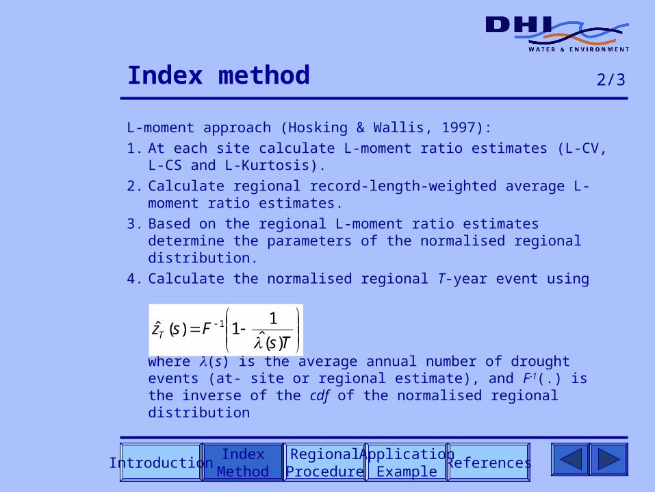
4. Calculate the normalised regional T-year event using

where (s) is the average annual number of drought events (at- site or regional estimate), and F-1(.) is the inverse of the cdf of the normalised regional distribution

IndexMethod

RegionalProcedure


Introduction

2/3

TsFszT

)(ˆ1

1)(ˆ 1

Index method

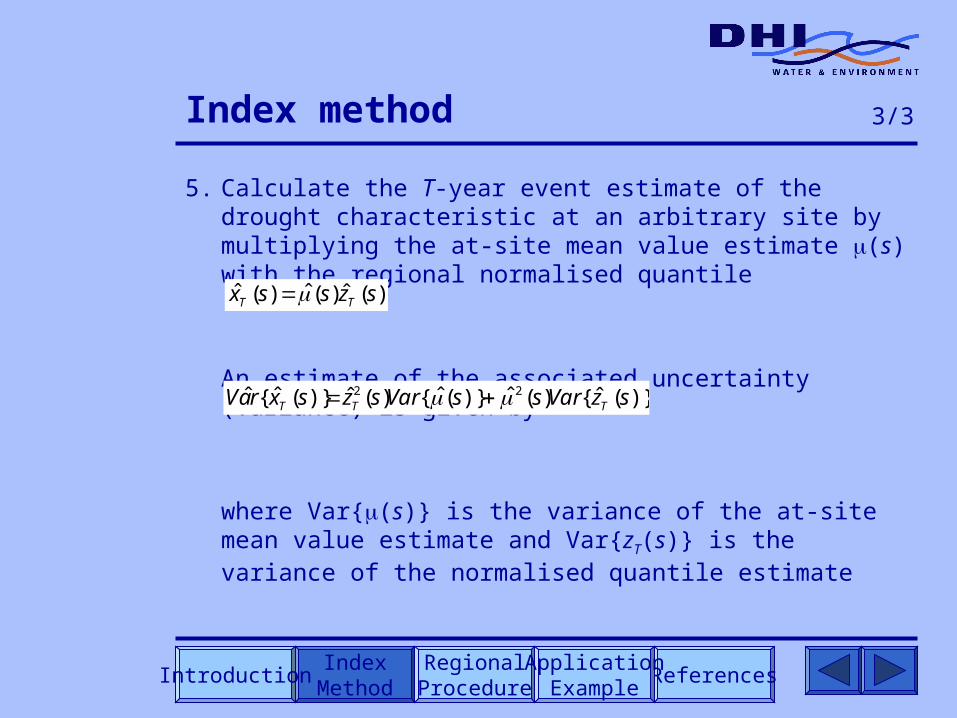
5. Calculate the T-year event estimate of the drought characteristic at an arbitrary site by multiplying the at-site mean value estimate (s) with the regional normalised quantile

An estimate of the associated uncertainty (variance) is given by

where Var{(s)} is the variance of the at-site mean value estimate and Var{zT(s)} is the variance of the normalised quantile estimate

IndexMethod

RegionalProcedure


Introduction

3/3

)(ˆ)(ˆ)(ˆ szssx TT

)}(ˆ{)(ˆ)}(ˆ{)(ˆ)}(ˆ{ˆ 22 szVarssVarszsxraV TTT

Regional procedure - outline

Building of the regional model includes:

1. Grouping of sites into homogeneous (or fairly homogeneous) regions.

2. Determination of a regional distribution in each of the defined regions.

3. Estimation of regional parameters (L-Cv and L-Cs) and associated uncertainties.

4. Determination of regression model that relates the mean value with catchment characteristics.

IndexMethod

RegionalProcedure


Outline

L-momentAnalysis

GLSRegression

Introduction

1/2

Split SampleGrouping

Regional procedure - outline

Tools available for the regional analysis:

L-moment analysis

- testing of regional homogeneity

- determination of a regional distribution

Generalised least squares (GLS) regression

- estimation of regional parameters and associated uncertainties

- testing of regional homogeneity

- determination of regression model

Split sample grouping

- grouping of sites into homogenous regions

IndexMethod

RegionalProcedure


Outline

L-momentAnalysis

GLSRegression


Introduction

2/2

L-moment analysis

Objective:

L-moment analysis is applied for testing regional homogeneity and determination of a regional distribution.

L-moment ratio diagram:

For a visual judgement an L-moment ratio diagram is constructed. In an L-moment ratio diagram sample estimates of the L-moment ratios L-Cv, L-Cs and L-kurtosis are compared to the theoretical relationships for a range of probability distributions.

L-moment statistics:

For a more formal evaluation Hosking and Wallis (1993) proposed a test statistic for regional homogeneity and a goodness-of-fit statistic for determination of a regional distribution.

IndexMethod

RegionalProcedure


Outline

L-momentAnalysis

GLSRegression

Introduction


1/11

L-moment ratio diagram

L-moment ratio diagram illustrating the relationship between L-skewness and L-kurtosis for the generalised Pareto (GP), generalised extreme value (GEV), log-normal (LN), gamma (GAM), Weibull (WEI), Gumbel (GUM) and exponential (EXP) distributions.

IndexMethod

RegionalProcedure


Outline

L-momentAnalysis

GLSRegression

-0.1

0.0

0.1

0.2

0.3

0.4

0.5

0 0.1 0.2 0.3 0.4 0.5 0.6L-skewness

L-ku

rtos

isGP GEV

LN GAM

WEI EXP

GUM

Introduction


2/11

L-moment ratio diagram

IndexMethod

RegionalProcedure


Outline

L-momentAnalysis

GLSRegression

L-moment ratio diagram illustrating the relationship between L-Cv and L-skewness for the two-parameter generalised Pareto (GP), log-normal (LN), gamma (GAM), and Weibull (WEI) distributions and the one-parameter exponential (EXP) distribution.

0.2

0.3

0.4

0.5

0.6

0.7

0.8

0 0.1 0.2 0.3 0.4 0.5 0.6L-skewness

L-C

VGP

LN

GAM

WEI

EXP

Introduction


3/11

Test of regional homogeneity

The dispersion of points in the L-moment diagram of the L-moment estimates from the different sites in the region gives an indication of the regional homogeneity. The question is if the observed variability is significant (i.e. the points form a heterogeneous group) or can be explained by sampling uncertainties.

IndexMethod

RegionalProcedure


Outline

L-momentAnalysis

GLSRegression

Introduction


4/11

-0.1

0.0

0.1

0.2

0.3

0.4

0.5

0 0.1 0.2 0.3 0.4 0.5 0.6L-skewness

L-ku

rtos

isGPGEVLNGAMWEIEstimatesAverage


Regional homogeneity measure:

Comparison of observed regional variability of L-moment statistics with the variability that would be expected in a homogeneous region.

IndexMethod

RegionalProcedure


Outline

L-momentAnalysis

GLSRegression

Introduction


5/11

0.2

0.3

0.4

0.5

0.6

0.7

0.0 0.1 0.2 0.3 0.4 0.5L-skewness

L-C

V

0.2

0.3

0.4

0.5

0.6

0.7

0.0 0.1 0.2 0.3 0.4 0.5L-skewness

L-C

V

Observed Simulated


Test statistic:

where V is the record-length-weighted standard deviation of the L-CV estimates, and v and v are, respectively, the mean and standard deviation of V in a homogeneous region (determined by simulation).

Evaluation of H-statistic:

H < 1: Acceptably homogeneous region

1 < H < 2: Possibly heterogeneous region

H > 2: Definitely heterogeneous region

IndexMethod

RegionalProcedure


Outline

L-momentAnalysis

GLSRegression

Introduction


6/11

V

V = V

H

Choice of regional distributionThe grouping of points in the L-moment ratio diagram is compared with the theoreticalL-moment relationships for a number of candidate distributions. To discriminate between different 3-parameter distributions the L-skewness/L-kurtosis diagram is used. TheL-Cv/L-skewness diagram is used to discriminate between various 2-parameter distributions.

IndexMethod

RegionalProcedure


Outline

L-momentAnalysis

GLSRegression

Introduction


7/11

-0.1

0.0

0.1

0.2

0.3

0.4

0.5

0 0.1 0.2 0.3 0.4 0.5 0.6L-skewness

L-ku

rtos

isGPGEVLNGAMWEIEstimatesAverage

Choice of regional distribution

Goodness-of-fit measure for a 3-parameter distribution:

Comparison of regional average L-kurtosis and the theoretical L-kurtosis for the considered distribution corresponding to the regional average L-skewness.

IndexMethod

RegionalProcedure


Outline

L-momentAnalysis

GLSRegression

Introduction


8/11

0.0

0.1

0.2

0.3

0.4

0.1 0.2 0.3 0.4 0.5L-skewness

L-ku

rtos

is

GEV

Weighted average


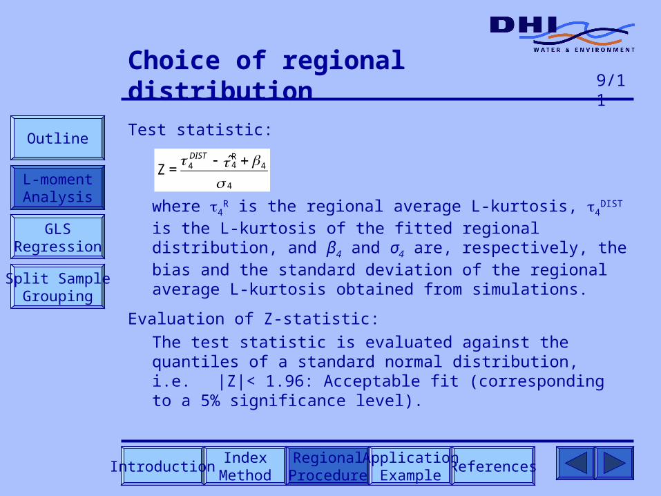
Test statistic:

where 4R is the regional average L-kurtosis, 4

DIST is the L-kurtosis of the fitted regional distribution, and β4 and σ4 are, respectively, the bias and the standard deviation of the regional average L-kurtosis obtained from simulations.

Evaluation of Z-statistic:

The test statistic is evaluated against the quantiles of a standard normal distribution, i.e. |Z|< 1.96: Acceptable fit (corresponding to a 5% significance level).

IndexMethod

RegionalProcedure


Outline

L-momentAnalysis

GLSRegression

Introduction


9/11

4

4R44 ˆ

= ZDIST


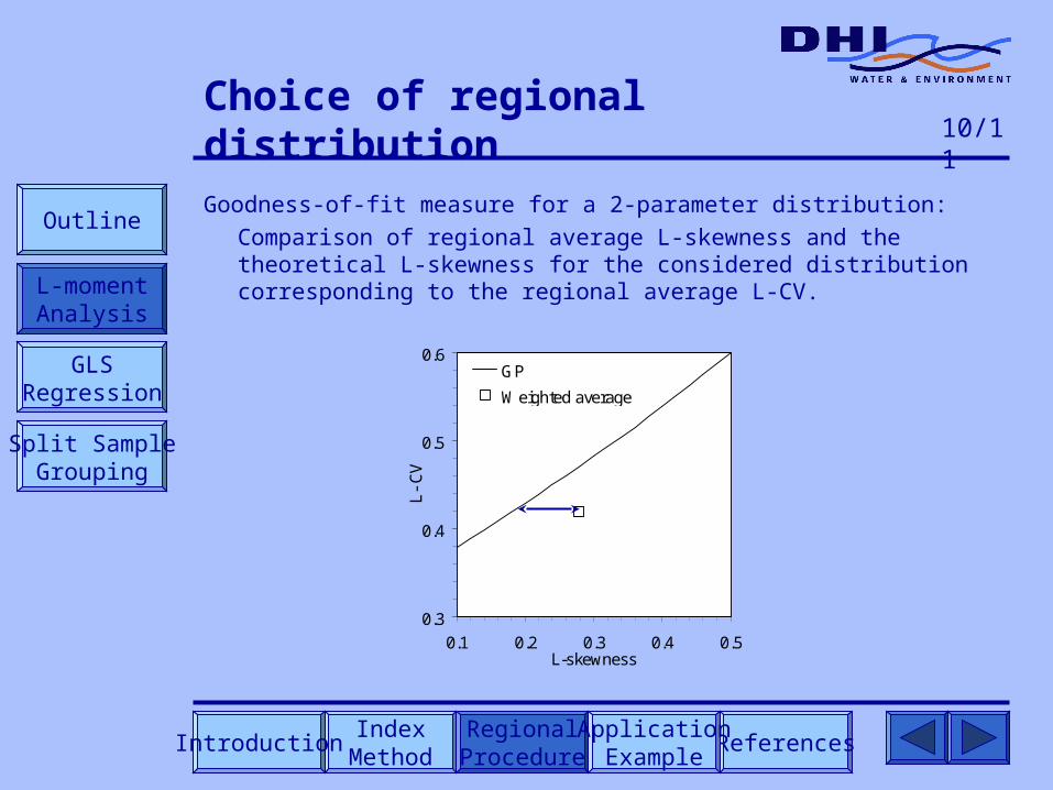
Goodness-of-fit measure for a 2-parameter distribution:

Comparison of regional average L-skewness and the theoretical L-skewness for the considered distribution corresponding to the regional average L-CV.

IndexMethod

RegionalProcedure


Outline

L-momentAnalysis

GLSRegression

Introduction


10/11

0.3

0.4

0.5

0.6

0.1 0.2 0.3 0.4 0.5L-skewness

L-C

V

GP

Weighted average


Test statistic:

where 3R is the regional average L-skewness, 3

DIST is the L-skewness of the fitted regional distribution, and σ3 is the standard deviation of the regional average L-skewness obtained from simulations.

Evaluation of Z-statistic:

The test statistic is evaluated against the quantiles of a standard normal distribution, i.e. |Z|< 1.96: Acceptable fit (corresponding to a 5% significance level).

IndexMethod

RegionalProcedure


Outline

L-momentAnalysis

GLSRegression

3

R33 ˆ

= ZDIST

Introduction


11/11

GLS regression

Objective:

Generalised least squares (GLS) regression is applied for estimation of regional parameters and testing of regional homogeneity. For parameters that show a significant regional variability the GLS regression procedure is subsequently applied to evaluate the potential of describing the variability from catchment characteristics (Stedinger & Tasker, 1985; Madsen & Rosbjerg, 1997).

IndexMethod

RegionalProcedure


Outline

L-momentAnalysis

GLSRegression

Introduction


1/6

Regional mean model

The regional mean model is a special case of the GLS regression model. It is used for estimation of regional parameters of L-moment ratios (L-Cv and L-Cs) and their associated uncertainties. In addition, the regional mean model provides a heterogeneity measure for testing regional homogeneity.

Input:

- L-moment ratio estimates L-Cv and L-Cs.

- Sampling variances of L-Cv and L-Cs estimates.

Output:

- Regional L-moment ratio estimates.

- Variance of regional L-moment ratio estimates.

- Residual model error variance (heterogeneity measure).

IndexMethod

RegionalProcedure


Outline

L-momentAnalysis

GLSRegression

Introduction


2/6

Regression model

The GLS regression model is used for estimation of mean drought statistics from catchment characteristics.

The following log-linear model is considered:

where i is the mean value of the drought characteristic, Aik are the considered catchment characteristics, k are the regression parameters, i is a random sampling error, and i is the residual model error.

IndexMethod

RegionalProcedure


Outline

L-momentAnalysis

GLSRegression

Introduction


3/6

i

p

1kikk0i )ln(A)ˆln(

i

Regression model

The sampling error and the residual model error are assumed to have zero mean and covariance structures

where 2i is the sampling error variance, ij is the correlation

coefficient due to concurrent observations at stations i and j (intersite correlation coefficient), and 2

is the residual model error variance.

Note: Compared to ordinary least squares regression GLS regression accounts explicitly for heteroscedastic (different variances) and cross-correlated sampling errors.

IndexMethod

RegionalProcedure


Outline

L-momentAnalysis

GLSRegression

Introduction


4/6

ji,0

ji,},{;

ji,

ji,},{

2

jiijji

2i

ji

CovCov

Regression model

Input:

- Mean value and associated variance of drought characteristic

- Catchment characteristics

Output:

- Regression parameters and associated covariance

- Residual model error variance

Application:

For given catchment characteristics the mean value and the associated variance are estimated from the GLS regression equation.

IndexMethod

RegionalProcedure


Outline

L-momentAnalysis

GLSRegression

Introduction


5/6

Regression model

In the case where some at-site data are available the sample mean AS and the mean value obtained from the regression equation R can be combined using (Madsen & Rosbjerg, 1997):

where Var{AS} is the variance of the at-site estimate and Var{R} is the variance of the regional estimate obtained from the regression model.

The variance of the weighted estimator is:

IndexMethod

RegionalProcedure


Outline

L-momentAnalysis

GLSRegression

Introduction


6/6

}ˆ{}ˆ{

}ˆ{,ˆ)1(ˆ)(ˆ

RAS

ASASR

VarVar

Varwwws

}ˆ{)}(ˆ{ RwVarsVar


Objective:

Grouping of sites into homogeneous (or fairly homogeneous) regions according to catchment characteristics.

Procedure (Wiltshire, 1995):

1. The method splits a set of catchments into two groups based on a single partitioning value of one chosen catchment characteristic. Measures of variability of drought characteristics within each group are aggregated into one statistic, and the optimum grouping is achieved at the point where this statistic is minimum.

2. Step 1 is repeated for all the considered catchment characteristics. The catchment characteristic that provides the minimum variability statistic is chosen as the optimal two-way grouping.

IndexMethod

RegionalProcedure


Outline

L-momentAnalysis

GLSRegression


Introduction

1/2


3. Steps 1-2 are repeated for a multiple partitioning, i.e. a four-way grouping based on 2 characteristics, an eight-way grouping based on 3 characteristics etc.

4. After each split sample grouping regional homogeneity is tested using the L-moment H-statistic or the GLS regression statistic.

Variability measure (Pearson, 1991; Madsen et al., 1997):

where ej,i is the deviation of the jth L-moment ratio estimate at site i from its group record-length-weighted average. In this case the L-Cv is weighted ahead of the L-skewness, which in turn is weighted ahead of L-kurtosis, so that homogeneity is primarily influenced by L-Cv and less so by L-kurtosis.

IndexMethod

RegionalProcedure


Outline

L-momentAnalysis

GLSRegression


Introduction

2/2

ii

iiiii

n

eeenV

2,4

2,3

2,2 23

Application example - data

The regional frequency analysis procedure was applied to the regional data set with daily streamflow series from Baden-Würtenberg, Germany

IndexMethod

RegionalProcedure


Data

Groupingof Sites

GLSRegression

QuantileEstimation

Introduction

1/6

Freiburg

Stuttgart

Karlsruhe

Strassburg (France)

Basel (Switzerland)

RegionalDistribution

Streamflow drought series

Streamflow data:

Stations with a record length larger than 20 years were included in the regional analysis, which comprises 46 stations with recording periods ranging between 20 to 37 years with an average of 30.2 years.

Drought series:

For definition of drought events the threshold level approach was applied using the 70% quantile of the daily flow duration curve as the threshold level (Tallaksen et al., 1997). From the drought series annual maximum series of drought duration and deficit volume were extracted. Of the 46 stations, 20 stations experience no zero drought years, whereas the remaining 26 stations have one or more zero drought years. The regional average annual number of drought events is equal to 0.952 years-1.

IndexMethod

RegionalProcedure


Data

Groupingof Sites

GLSRegression

QuantileEstimation

Introduction

2/6



Empirical distributions of AMS of drought duration

IndexMethod

RegionalProcedure


Data

Groupingof Sites

GLSRegression

QuantileEstimation

Introduction

3/6

0

50

100

150

200

250

300

350

400

450

500

1 10 100Return period [years]

Dur

atio

n [d

ays]


0

20

40

60

80

100

120

140

160

180

1 10 100Return period [years]

Def

icit

volu

me

[mm

]


Empirical distributions of AMS of deficit volume (normalised with the catchment area)

IndexMethod

RegionalProcedure


Data

Groupingof Sites

GLSRegression

QuantileEstimation

Introduction

4/6


Catchment characteristics

Climate:

Mean annual precipitation [mm]

Land use:

Fraction of urbanisation [-]Fraction of forest [-]

Morphometry:

Catchment area [km2]Drainage density [km/ km2]Highest elevation [m a.m.s.l.]Average elevation [m a.m.s.l.]Lowest elevation [m a.m.s.l.]Maximum slope [%]Average slope [%]Minimum slope [%]

IndexMethod

RegionalProcedure


Data

Groupingof Sites

GLSRegression

QuantileEstimation

Introduction

5/6


Catchment characteristics

Soil:

Fraction of soils with high infiltration capacity [-]Fraction of soils with medium infiltration capacity [-]Fraction of soils with low infiltration capacity [-]Fraction of soils with very low infiltration capacity [-]Mean hydraulic conductivity of the soils [cm/d]Fraction of soils with low hydraulic conductivity [-]Fraction of soils with high water-holding capacity in the effective root zone [-]Mean water-holding capacity in the effective root zone [mm]

Hydrogeology:Fraction of rock formations with a very low hydraulic permeability [%]Weighted mean of hydraulic conductivity [m/s]

IndexMethod

RegionalProcedure


Data

Groupingof Sites

GLSRegression

QuantileEstimation

Introduction

6/6


Grouping of sites

Testing of regional homogeneity of all 46 catchments:

Duration: H = 5.76

Deficit volume: H = 4.08

Both for duration and deficit volume the H-statistic indicates that all 46 catchments form a “definitely heterogeneous” group with respect to L-Cv.

Split sample grouping (two-way grouping):

The global minimum value of the variability statistic V as a function of the different catchment characteristics is obtained with the mean annual precipitation (MAP).

“Dry catchments”: MAP < 1000 mm

“Wet catchments”: MAP > 1000 mm

IndexMethod

RegionalProcedure


Data

Groupingof Sites

GLSRegression

Introduction

QuantileEstimation

1/10


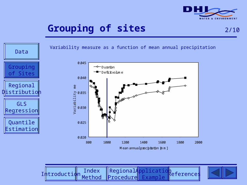
Grouping of sites

Variability measure as a function of mean annual precipitation

IndexMethod

RegionalProcedure


Data

Groupingof Sites

GLSRegression

Introduction

QuantileEstimation

0.020

0.025

0.030

0.035

0.040

0.045

800 1000 1200 1400 1600 1800 2000

Mean annual precipitation [mm]

Var

iabi

lity

mea

sure

Duration

Deficit volume

2/10


Grouping of sites

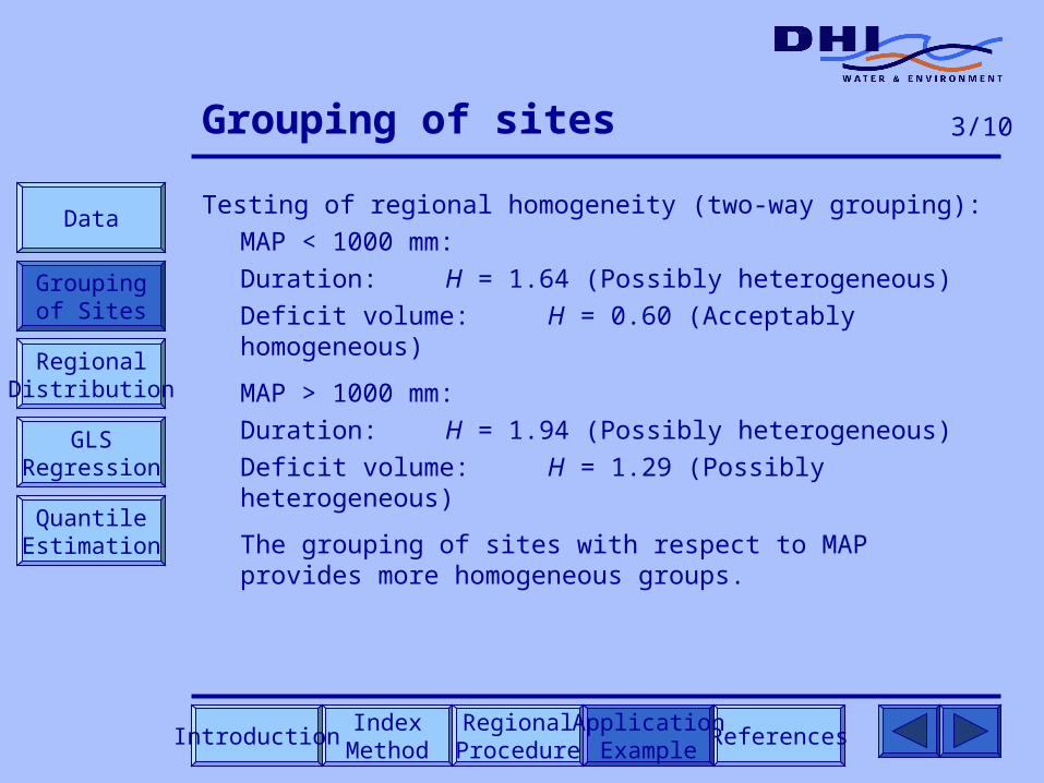
Testing of regional homogeneity (two-way grouping):

MAP < 1000 mm:

Duration: H = 1.64 (Possibly heterogeneous)

Deficit volume: H = 0.60 (Acceptably homogeneous)

MAP > 1000 mm:


Deficit volume: H = 1.29 (Possibly heterogeneous)

The grouping of sites with respect to MAP provides more homogeneous groups.

IndexMethod

RegionalProcedure


Data

Groupingof Sites

GLSRegression

Introduction

QuantileEstimation

3/10


Grouping of sites

Split sample grouping (four-way grouping):

MAP < 1000 mm:

For the “dry catchment” group the available catchment characteristics did not provide a well-defined partitioning.

MAP > 1000 mm:

For the “wet” catchments a well-defined partitioning was obtained with the catchment average hydraulic conductivity of the upper hydrogeological unit (HCMEAN) with a minimum variability measure for HCMEAN = 2.510-5 m/s.

IndexMethod

RegionalProcedure


Data

Groupingof Sites

GLSRegression

Introduction

QuantileEstimation

4/10


Grouping of sites

Variability measure as a function of average hydraulic conductivity

IndexMethod

RegionalProcedure


Data

Groupingof Sites

GLSRegression

Introduction

QuantileEstimation

0.020

0.021

0.022

0.023

0.024

0.025

0.026

0.027

0.028

0.0E+00 1.0E-05 2.0E-05 3.0E-05 4.0E-05 5.0E-05 6.0E-05

Average hydraulic conductivity [m/s]

Var

iabi

lity

mea

sure

Duration

Deficit volume

5/10


Grouping of sites

Testing of regional homogeneity (four-way grouping):

Region A (MAP < 1000 mm):


Deficit volume: H = 0.60 (Acceptably homogeneous)

Region B (MAP > 1000 mm, HCMEAN < 2.510-5 m/s):

Duration: H = -2.12 (Acceptably homogeneous)

Deficit volume: H = -0.36 (Acceptably homogeneous)

Region C (MAP > 1000 mm, HCMEAN > 2.510-5 m/s):

Duration: H = 0.24 (Acceptably homogeneous)

Deficit volume: H = -0.64 (Acceptably homogeneous)

IndexMethod

RegionalProcedure


Data

Groupingof Sites

GLSRegression

Introduction

QuantileEstimation

6/10


Grouping of sites

L-Cv and L-Cs estimates of the three regions for drought duration

IndexMethod

RegionalProcedure


Data

Groupingof Sites

GLSRegression

Introduction

QuantileEstimation

0.2

0.3

0.4

0.5

0.6

0.7

0.8

0 0.1 0.2 0.3 0.4 0.5 0.6L-skewness

L-C

V

GP LNGAM WEIRegion A Avg. Region ARegion B Avg. Region BRegion C Avg. Region C

7/10


0.2

0.3

0.4

0.5

0.6

0.7

0.8

0 0.1 0.2 0.3 0.4 0.5 0.6L-skewness

L-C

V

GP LNGAM WEIRegion A Avg. Region ARegion B Avg. Region BRegion C Avg. Region C

Grouping of sites

L-Cv and L-Cs estimates of the three regions for deficit volume

IndexMethod

RegionalProcedure


Data

Groupingof Sites

GLSRegression

Introduction

QuantileEstimation

8/10


-0.1

0.0

0.1

0.2

0.3

0.4

0.5

0 0.1 0.2 0.3 0.4 0.5 0.6L-skewness

L-k

urt

osi

s

GP GEVLN GAMWEI Region AAvg. Region A Region BAvg. Region B Region CAvg. Region C

Grouping of sites

L-Cs and L-kurtosis estimates of the three regions for duration

IndexMethod

RegionalProcedure


Data

Groupingof Sites

GLSRegression

Introduction

QuantileEstimation

9/10


-0.1

0.0

0.1

0.2

0.3

0.4

0.5

0 0.1 0.2 0.3 0.4 0.5 0.6L-skewness

L-k

urt

osi

s

GP GEVLN GAMWEI Region AAvg. Region A Region BAvg. Region B Region CAvg. Region C

Grouping of sites

L-Cs and L-kurtosis estimates of the three regions for deficit volume

IndexMethod

RegionalProcedure


Data

Groupingof Sites

GLSRegression

Introduction

QuantileEstimation

10/10


Goodness-of-fit statistics

Duration (3-parameter distribution):

Duration (2-parameter distribution):

IndexMethod

RegionalProcedure


Data

Groupingof Sites


GLSRegression

Introduction

QuantileEstimation

1/7

Distributions accepted at a 5% significance level marked in red


Deficit volume (3-parameter distribution):

Deficit volume (2-parameter distribution):

IndexMethod

RegionalProcedure


Data

Groupingof Sites

GLSRegression

Introduction

QuantileEstimation

2/7

Distributions accepted at a 5% significance level marked in redRegional

Distribution


Distributions accepted at a 5% significance level:

3-parameter distributions (out of 3 regions):

GP: Duration: 2; Volume: 1GEV: Duration: 0; Volume: 0LN: Duration: 0; Volume: 0GAM: Duration: 2; Volume: 2WEI: Duration: 2; Volume: 2

2-parameter distributions (out of 3 regions):

GP: Duration: 2; Volume: 0LN: Duration: 0; Volume: 0GAM: Duration: 2; Volume: 3WEI: Duration: 1; Volume: 2

2-parameter Gamma distribution chosen for both duration and volume in all 3 regions.

IndexMethod

RegionalProcedure


Data

Groupingof Sites

GLSRegression

Introduction

QuantileEstimation

3/7


Regional parameters

Regional parameters (duration):

Regional parameters (deficit volume):

IndexMethod

RegionalProcedure


Data

Groupingof Sites

GLSRegression

Introduction

QuantileEstimation

4/7


Normalised regional distributions

The regional L-Cv estimates and average annual number of drought events (average rates) are used to estimate the normalised regional quantile in the three regions for both drought duration and deficit volume.

Region A catchments have heavier tailed distributions than the Region C catchments, which in turn have heavier tailed distributions than the Region B catchments. In each region the deficit volume have heavier tailed distributions than the duration.

IndexMethod

RegionalProcedure


Data

Groupingof Sites

GLSRegression

Introduction

QuantileEstimation

5/7



Drought duration

IndexMethod

RegionalProcedure


Data

Groupingof Sites

GLSRegression

Introduction

QuantileEstimation

0.0

2.0

4.0

6.0

8.0

10.0

1 10 100 1000

Return period [years]

Nor

mal

ised

qua

ntile

Region A

Region B

Region C

6/7


0.0

2.0

4.0

6.0

8.0

10.0

1 10 100 1000


Nor

mal

ised

qua

ntileRegion A

Region B

Region C


Deficit volume

IndexMethod

RegionalProcedure


Data

Groupingof Sites

GLSRegression

Introduction

QuantileEstimation

7/7


GLS estimation of L-Cv

To further analyse the regional homogeneity and estimate the uncertainty of the regional L-Cv estimate the GLS regional mean model is applied.

Results for drought duration:

IndexMethod

RegionalProcedure


Data

Groupingof Sites


GLSRegression

Introduction

QuantileEstimation

1/9


Results for deficit volume:

IndexMethod

RegionalProcedure


Data

Groupingof Sites

GLSRegression

Introduction

QuantileEstimation

2/9



The residual model error variance can be used to assess regional homogeneity. In this case only Region B for drought duration and Region C for deficit volume can be assumed homogeneous (residual model error variance = 0). This contradicts the results of the H-statistic where only Region A for duration was flagged as possibly heterogeneous and illustrates the lack of power of the H-statistic in the case of significant intersite correlation as observed in this case.

The estimated variance of the regional L-Cv estimator can be used to produce confidence bands on the regional normalised frequency curve. In this case the uncertainty of the regional quantile estimate can be obtained by Monte Carlo simulation of a gamma distribution using a normal distribution of the regional L-Cv estimator.

IndexMethod

RegionalProcedure


Data

Groupingof Sites

GLSRegression

Introduction

QuantileEstimation

3/9



Normalised regional frequency curve for deficit volume in Region B with associated 95% confidence limits

IndexMethod

RegionalProcedure


Data

Groupingof Sites

GLSRegression

Introduction

QuantileEstimation

0.0

2.0

4.0

6.0

8.0

10.0

10 100 1000


Nor

mal

ised

qua

ntile

Regional estimate

95% confidence limits

4/9


GLS estimation of mean value

For quantile estimation at an ungauged site an estimate of the mean drought duration and deficit volume is needed. In addition, if only a short record is available at the considered site the sample mean and the regional estimate of the mean value can be combined to obtain a more reliable estimate.

For estimation of the mean drought characteristics log-linear regression models that relate the mean duration and deficit volume to the catchment characteristics for the three different regions are evaluated using the GLS regression procedure.

IndexMethod

RegionalProcedure


Data

Groupingof Sites

GLSRegression

Introduction

QuantileEstimation

5/9



The GLS regression procedure was applied using all combinations of the catchment characteristics. To evaluate the predictive capabilities of the different regression models the average mean square error (MSE) of prediction is used as a performance index.

The model that produces the smallest average MSE is generally chosen. However, taken the principle of model parsimony into account, if only a minor improvement is obtained by including an additional catchment characteristic, that characteristic is not included.

IndexMethod

RegionalProcedure


Data

Groupingof Sites

GLSRegression

Introduction

QuantileEstimation

6/9



Results for drought duration:

Region A:

Region B:

Region C:

IndexMethod

RegionalProcedure


Data

Groupingof Sites

GLSRegression

Introduction

QuantileEstimation

EAN)ln(SOILHCM1996.0

SOILL)1ln(498.0FOREST)1ln(697.0761.3)ln(

AN)ln(ROOTSME024.1830.8)ln(

ROOTSHIGH)1ln(487.3

ln(DD)2101.0SOILL)1ln(5813.0967.3)ln(

7/9



Results for deficit volume:

Region A:

Region B:

Region C:

IndexMethod

RegionalProcedure


Data

Groupingof Sites

GLSRegression

Introduction

QuantileEstimation

EAN)ln(SOILHCM204.1

SOILL)1ln(512.1FOREST)1ln(436.1873.1)ln(

ln(MAP)675.2ln(DD)7485.047.16)ln(

ln(MAP)752.2ln(DD)2793.001.17)ln(

8/9



Catchment descriptors used in regression equations:

FOREST: Fraction of forest [-]

SOILL: Fraction of soils with low infiltration capacity [-]

SOILHCMEAN: Mean hydraulic conductivity of the soils [cm/day]

ROOTSMEAN: Mean water-holding capacity in the effective root zone [mm]

DD: Drainage density [km/km2]

ROOTSHIGH: Fraction of soils with high water-holding capacity in the effective root zone [-]

MAP: Mean annual precipitation [mm].

IndexMethod

RegionalProcedure


Data

Groupingof Sites

GLSRegression

Introduction

QuantileEstimation

9/9


Regional quantile estimation

1. Based on MAP and HCMEAN at the considered site, the catchment is assigned a region (A, B or C) with specified normalised frequency curve and associated variance.

2. Based on additional catchment characteristics the mean drought duration and deficit volume are obtained from the regression equations together with an estimate of the associated variance.

3. If data are available at the considered site, the at-site mean duration and deficit volume are estimated. These estimates are combined with the regression estimates using the weighted estimator described in Regional Procedure - GLS Regression.

4. The T-year drought duration and deficit volume are obtained by multiplying the estimated mean values with the normalised quantile estimate. The quantile estimate and associated variance are described in Index Method.

IndexMethod

RegionalProcedure


Data

Groupingof Sites

GLSRegression

QuantileEstimation

Introduction

1/1


References

Hosking, J.R.M. & Wallis, J.R. (1993) Some statistics useful in regional frequency analysis, Water Resour. Res., 29(2), 271-281. Correction, Water Resour. Res., 31(1), 251, 1995.

Hosking, J.R.M. & Wallis, J.R. (1997) Regional Frequency Analysis, An Approach Based on L-moments, Cambridge University Press, UK.

Madsen, H. & Rosbjerg, D. (1997) Generalized least squares and empirical Bayes estimation in regional partial duration series index-flood modeling, Water Resour. Res., 33(4), 771-781.

Madsen, H., Pearson, C.P. & Rosbjerg, D. (1997) Comparison of annual maximum series and partial duration series for modeling extreme hydrologic events, 2. Regional modelling, Water Resour. Res., 33(4), 759-769.

Pearson, C.P. (1991) New Zealand regional flood frequency analysis using L-moments, J. Hydrol. NZ, 30(2), 53-64.

IndexMethod

RegionalProcedure


Introduction

1/2

References

Stedinger, J.R. & Tasker, G.D. (1985) Regional hydrologic analysis, 1. Ordinary, weighted and generalized least squares compared, Water Resour. Res., 21(9), 1421-1432. Correction, Water Resour. Res., 22(5), 844, 1986.

Tallaksen, L.M., Madsen, H. & Clausen, B. (1997) On the definition and modelling of streamflow drought duration and deficit volume, Hydrol. Sci. J., 42(1), 15-33.

Wiltshire, S.E. (1985) Grouping basins for regional flood frequency analysis, Hydrol. Sci. J., 30(1), 151-159.

IndexMethod

RegionalProcedure


Introduction

2/2

End

regional frequency analysis of hydrological droughts henrik madsen dhi water & environment

Documents

regional estimate

regional data

regional normalised

regional recordlength

index method assumptions

drought statistics

site mean value estimate

moment ratio estimates