African

Develop

ment Ba

nk Grou

p

Regional Financial Integrationand Economic Activity in Africa

Working

Pape

r Serie

s

Akpan Ekpo and Chuku Chuku

Integ

rate A

frica

n° 29

1

Septe

mber 2

017

4

Working Paper No 291

Abstract Unlike in Asia and Europe, it is not clear what the pattern and impact of financial integration have been in Africa. This paper addresses three main issues: the progress and experience towards financial integration in Africa, the degree and timing of the integration process in selected African stock markets, and the effect of financial integration on economic activity. First, using time-varying parameters from a state-space model, we assess the degree and timing of financial integration in Africa and find results that indicate contemporary patterns toward increasing financial globalisation relative to

regionalization. Second, using carefully specified parametric and nonparametric regression analyses, we find that higher levels of financial integration is associated with higher levels of growth and investment, but not necessarily total factor productivity. The relationships become even clearer when we zoom in on the nonparametric iso-growth surface plots, which show that there is a threshold level of financial development that is consistent with growth in a financially segmented economy. Finally, some policy implications are gleaned from the results and the experiences in Asia and Europe.

Rights and Permissions

All rights reserved.

The text and data in this publication may be reproduced as long as the source is cited. Reproduction for commercial purposes

is forbidden. The WPS disseminates the findings of work in progress, preliminary research results, and development

experience and lessons, to encourage the exchange of ideas and innovative thinking among researchers, development

practitioners, policy makers, and donors. The findings, interpretations, and conclusions expressed in the Bank’s WPS are

entirely those of the author(s) and do not necessarily represent the view of the African Development Bank Group, its Board

of Directors, or the countries they represent.

Working Papers are available online at https://www.afdb.org/en/documents/publications/working-paper-series/

Produced by Macroeconomics Policy, Forecasting, and Research Department

Coordinator

Adeleke O. Salami

This paper is the product of the Vice-Presidency for Economic Governance and Knowledge Management. It is part of a larger effort by the African Development Bank to promote knowledge and learning, share ideas, provide open access to its research, and make a contribution to development policy. The papers featured in the Working Paper Series (WPS) are those considered to have a bearing on the mission of AfDB, its strategic objectives of Inclusive and Green Growth, and its High-5 priority areas—to Power Africa, Feed Africa, Industrialize Africa, Integrate Africa and Improve Living Conditions of Africans. The authors may be contacted at workingpaper@afdb.org.

Correct citation: Ekpo, A., and C. Chuku (2017), Regional Financial Integration and Economic Activity in Africa, Working Paper Series N° 291, African Development Bank, Abidjan, Côte d’Ivoire.

Regional Financial Integration and Economic Activity in Africa1

Akpan Ekpo and Chuku Chuku

JEL Codes: F36, E44, C23, C14

Keywords: Financial integration, State-space model, Nonparametric regression, Economic activity, Africa

1 Professor Akpan Ekpo is a member of the Presidential Economic Management Team in Nigeria and the Director

General of the West African Institute for Financial and Economic Management (WAIFEM). Email: ahekpo@yahoo.com or ahekpo@waifem-cbp.org; Chuku Chuku is with the Department of Economics, University of Uyo, Nigeria; and a member of the Macroeconomic Modelling Team at the African Development Bank, Cote d’Ivoire. Email: chukuachuku@gmail.com or c.chuku@afdb.org.

The authors are grateful for the funding for this project provided by the African Economic Research Consortium (AERC) with Grant No. RC 13537. They also benefited from review comments by Lemma Senbet, Isaac Otchere, Robert Lensink, Kalu Ojah, Peter Quartly, and participants at the Plenary Session of the June 2016 AERC Biannual Workshop and various collaborative workshops. They would also like to thank Manuel Arellano and participants at the 2015 Econometric Society Conference in Zambia for useful comments on earlier versions. The paper is forthcoming in the Journal of African Economies.

1

1 Introduction

Financial development and integration became the prominent reform tools for most devel-

oping countries in the early 1980s when it became obvious that the lack of well-developed

financial systems was inhibiting progress in these countries. To fix ideas early, regional

financial integration refers to a market or institutionally driven process of broadening and

deepening the financial interrelationships within a region; whereas, financial development

refers to the process by which financial institutions and markets increase in size and influence

on the rest of the economy (Senbet, 1998; Wakeman-Linn & Wagh, 2008). This process

of financial regionalization involves several activities, the fundamental ones being: the

elimination of cross-country investment barriers; equitable treatment of foreign and domestic

investors; harmonization of national policies, laws, and institutions; synchronization of

operational structures like technology and information systems; and very importantly, the

convergence of prices, returns, and risk assessments.

Our aim in this study is threefold: first, to trace the progress and experience towards

financial integration in Africa, benchmarking the progress made so far on ex ante targets;

second, to determine the degree and timing of financial integration in selected sub-Saharan

African stock markets, using an unobserved latent variable; and finally, to understand the

effect of regional financial integration on economic activity in Africa, using both linear

parametric and nonlinear (nonparametric) estimation techniques. But why should markets,

especially those in Africa, be regionally integrated? Many authorities in the field have

endeavoured to answer this question by showing descriptively, and sometimes theoretically,

how this could be a strategic approach for Africa’s accelerated development and structural

transformation.1

Overall, it is expected that financial regionalization would enable the participating

regional economies to take advantage of the “systemic scale economies” that accrue to larger

financial systems. These scale effects emanate from several angles, including the expansion

of the spectrum of opportunities for financial intermediation; the creation of larger markets,

which makes it more cost effective to improve financial infrastructure; the efficiency effects

that arise from the increase in the number of financial sector participants, which promotes

diversification and healthy competition, and thus, eventually results in lower prices for

services; and lastly, the increased capacity to withstand financial crisis (see Wakeman-Linn

& Wagh, 2008; Senbet & Otchere, 2006; Agenor, 2003).

Moreover, financial integration generally improves macroeconomic and financial discipline.

Although there is historical evidence that greater financial integration could also have adverse

effects on the economy—for example, through the higher risk of cross-border financial

contagion, which was recently observed in the global financial crisis of 2007/08 and the

1Some examples include Senbet (1998); Ekpo (1994); Ali and Imai (2015); Senbet (2009); Ogunkola (2002);Chuku (2012); Senbet and Otchere (2006); Obadan (2006); Wakeman-Linn and Wagh (2008) and Ekpoand Afangide (2010)

2

Asian financial crisis of the late 1990s—there is a more stable relationship between financial

integration and economic growth (see Edison, Levine, Ricci, & Sløk, 2002). Other potential

costs of financial integration include uneven distribution of the flow of funds, which is often

skewed in favour of countries with larger markets; inadequate domestic allocation of the flow

of funds, which could hamper growth effects and exacerbate domestic distortions; loss of

macroeconomic stability; and the risks associated with the penetration of foreign financial

institutions (see Agenor, 2003; Park & Lee, 2011).

The problem, however, is that despite the highlighted benefits of financial integration to

participating economies—a fact that has been established for other regions using stylized

information and empirical analysis (see, for examples, Agenor (2003); Fung, Tam, and

Yu (2008); Edison et al. (2002); Baele, Ferrando, Hordahl, Krylova, and Monnet (2004),

and Adjaoute and Danthine (2004))—it is not obvious that this is also the case for Africa,

especially because of the peculiar idiosyncrasies of the existing regional financial architecture,

and the fact that there are hardly any studies that examine this relationship beyond a

correlation and descriptive statistics based framework. Hence, it is important to rigorously

investigate whether or not the extent of regional financial integration achieved so far has

helped to improve the level of aggregate economic activity in Africa. Insights from such an

investigation will provide an objective assessment of the growth impact of financial regional-

ization, and serve as a basis for rationalising any proposals for reforms and intensification of

the financial integration process in Africa.

This study contributes to the literature in at least three different ways. First, from a

methodological point of view, this is the first study we are aware of that uses nonpara-

metric estimation techniques to examine the effects of financial integration.2 Similarly,

the application of the Haldane and Hall (1991) type measure of convergence to gauge the

degree and timing of integration in African stock markets is also novel, to the best of our

knowledge. Secondly, unlike previous studies that try to justify regional financial integration

in Africa using theoretical and descriptive statistics (see for examples Senbet & Otchere,

2006; Wakeman-Linn & Wagh, 2008), our approach is based on a “cause–effect” identification

of the relationship using parametric and nonparametric techniques, thereby providing a

more scientific perspective on the issue. Thirdly, the study specifically focuses on African

economies and considers a broader set of control variables—particularly institutional and

governance variables—which are often ignored in several studies. This focus and emphasis

enable us to abstract from country- and regional-specific heterogeneity, thereby focusing

strictly on the African experience.

Overall, the key findings from our analysis reveal that there is increasing sensitivity

towards financial globalisation rather than regionalization. Also, we find evidence that an

improvement in regional financial integration is associated with higher GDP per capita

2Closely related applications of this methodology are Henderson and Millimet (2008), applied to the tradegravity literature; Henderson, Papageorgiou, and Parmeter (2012), in the growth empirics literature.

3

growth rates, and financial development only plays a complementary role up to a threshold.

Further, the growth enhancing effects of financial integration are stronger in countries with

lower levels of financial development; however, the impact is greater in countries with higher

levels of financial development. When using investment growth as a measure of economic

activity, we find that countries that are more regionally integrated enjoy higher levels of

capital investments. Generally, our results and conclusions survive well under alternative

estimation techniques and alternative measures of economic activity.

The balance of the paper is as follows. In Section 2, we provide a brief historical account

and status report of the progress towards financial integration in Africa. Section 3 contains

a review of the indicators of financial integration, with a brief motivation of the Haldane

and Hall state-space based measure of market convergence. In Section 4, we describe the

procedure for estimating the impact of financial integration and development on economic

activity; and Section 5 contains the results. In Section 6, we discuss the policy implications

of the results and draw lessons from the integration experiences in Asia and Europe. Section

7 concludes.

2 Africa’s experience in regional financial integration

The historic account of financial integration and cooperation in Africa is somewhat chequered

and dates back to the colonial days. The earliest record of efforts towards regionalization

was with the establishment of the Southern African Customs Union (SACU) in 1910, which

was later modified in 1969.3 Recent trends towards regionalization have now gone beyond

trade and customs unions to economic, financial, and monetary integration. Table 1 provides

a progress report on Africa’s integration processes. The progress report indicates that most

of the planned integration objectives along the lines of trade and tariff harmonisation have

been achieved. However, most of the integration targets in capital markets and economic

and monetary unions, which are based on the Abuja 1991 Treaty, have not yet been achieved

at the broader scope of the continent.

Current and future continent-wide efforts at strengthening financial regionalization is

being anchored by the African Union Commission (AUC) and the African Development

Bank (AfDB). One of the core proposals being pursued currently is the establishment of

three Pan-African financial institutions: the African Investment Bank (AIB), the African

Central Bank (ACB), and the African Monetary Fund (AMF), which is in line with the

Consultative Act of the AU (UNECA & AU, 2008). Although there is increasing progress

towards financial integration in Africa, financial market activities remain shallow, especially

in the sense that financial markets are still characterised by low capitalization, low liquidity,

short-term structure of instruments, and a limited number of financial instruments. Table 2

presents the structure of capital markets in Africa in terms of the scope of instruments

3SACU is noted to be the oldest customs union in the world (Wakeman-Linn & Wagh, 2008).

4

traded. We observe from the table that, as at 2012, 11 countries still had no capital markets,

and only 10 countries have capital markets that simultaneously trade in treasury bills,

sovereign bonds, corporate bonds, and equity markets.

Conversely, in the banking sub-sector, Africa has witnessed tremendous growth in the

last two decades driven mainly by African indigenous banks. Specifically, as at 2014, more

than 15 African indigenous banks had a presence in at least four or more countries. Among

the big pan-African players, the ones that grew significantly from 1990–2014 are Standard

Bank (from South Africa, increased operations from four countries to over 33 in the period);

Ecobank (from Togo, increased from five to over 30), United Bank of Africa (from Nigeria,

increased from two to over 20); and Bank of Africa (from Mali, increased from two to over

10) (see IMF, 2015). In East Africa, some Kenyan banks (for example, Kenya Commercial

Bank, Equity Bank, and Fina Bank), driven by the increasing integration process in East

Africa, are leading cross-border banking expansion (UNECA & AU, 2008; IMF, 2014). This

expansion by banks has greatly accelerated the pace of integration in the region, especially

because most of these banks are members of conglomerates that have operations in sectors

beyond banking, for example, in capital markets, insurance, microfinance, pensions, money

transfer, leasing and even in the non-financial sectors (see Allen, Otchere, & Senbet, 2011).

5

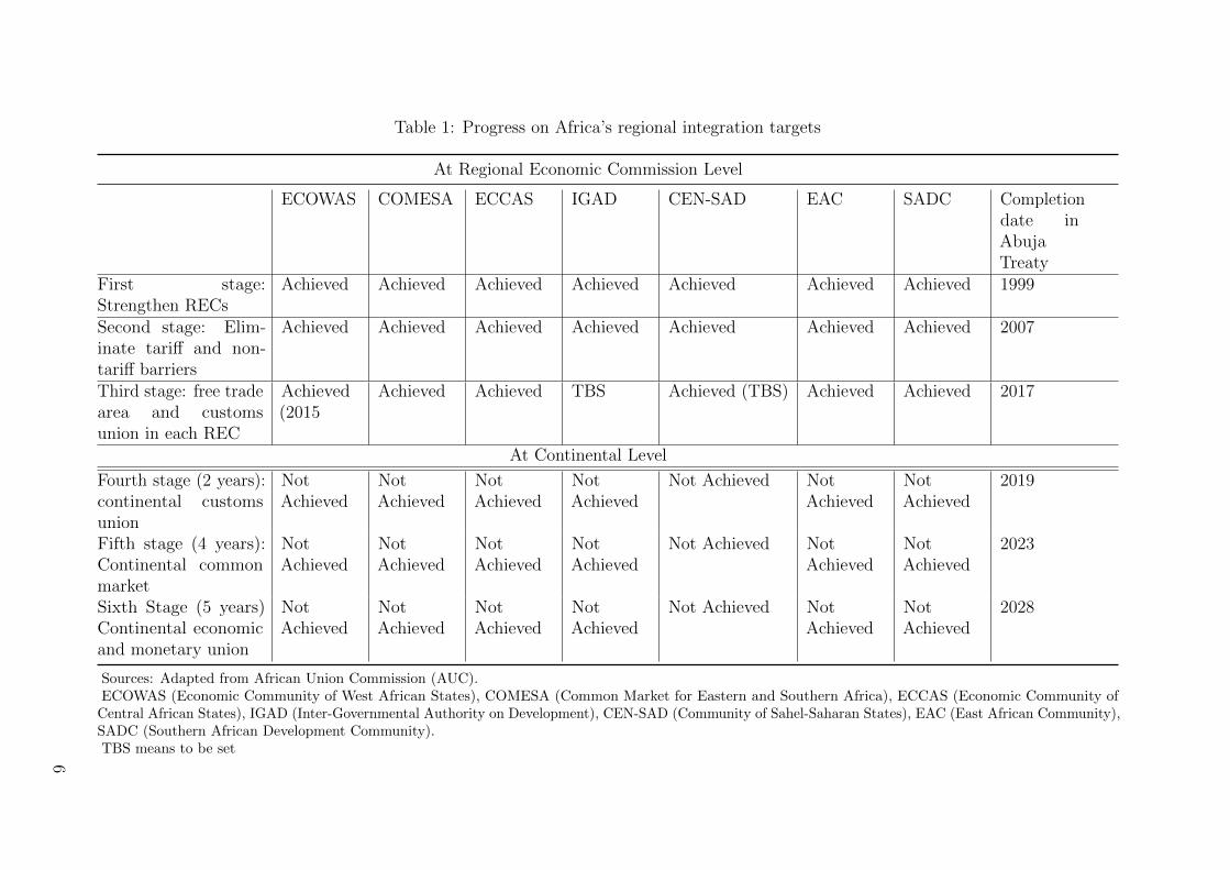
Table 1: Progress on Africa’s regional integration targets

At Regional Economic Commission Level

ECOWAS COMESA ECCAS IGAD CEN-SAD EAC SADC Completiondate inAbujaTreaty

First stage:Strengthen RECs

Achieved Achieved Achieved Achieved Achieved Achieved Achieved 1999

Second stage: Elim-inate tariff and non-tariff barriers

Achieved Achieved Achieved Achieved Achieved Achieved Achieved 2007

Third stage: free tradearea and customsunion in each REC

Achieved(2015

Achieved Achieved TBS Achieved (TBS) Achieved Achieved 2017

At Continental Level

Fourth stage (2 years):continental customsunion

NotAchieved

NotAchieved

NotAchieved

NotAchieved

Not Achieved NotAchieved

NotAchieved

2019

Fifth stage (4 years):Continental commonmarket

NotAchieved

NotAchieved

NotAchieved

NotAchieved

Not Achieved NotAchieved

NotAchieved

2023

Sixth Stage (5 years)Continental economicand monetary union

NotAchieved

NotAchieved

NotAchieved

NotAchieved

Not Achieved NotAchieved

NotAchieved

2028

Sources: Adapted from African Union Commission (AUC).ECOWAS (Economic Community of West African States), COMESA (Common Market for Eastern and Southern Africa), ECCAS (Economic Community of

Central African States), IGAD (Inter-Governmental Authority on Development), CEN-SAD (Community of Sahel-Saharan States), EAC (East African Community),SADC (Southern African Development Community).TBS means to be set

6

Table 2: Structure of capital markets in sub-Saharan Africa

(1) (2) (3) (4) (5)

# No Markets Treasury BillsMarket

(2) plus Trea-sury Bonds

(3) plus EquityMarkets

All four mar-kets

1 Burundi Congo Angola Benin Botswana2 Cen. Afr. Rep. Ethiopia Gambia Burkina Faso Ghana3 Chad Guinea Senegal Cameroon Kenya4 Comoros Guinea-Bissau Seychelles Cape Verde Namibia5 Congo D.R Lesotho Cote d’Ivoire Nigeria6 Eritrea Madagascar Gabon South Africa7 Equatorial

GuineaMalawi Mauritius Swaziland

8 Liberia Sierra Leone Mozambique Tanzania9 Mali Togo Rwanda Uganda10 Niger Zimbabwe Zambia11 S.T and P

Sources: Adapted from UNECA and AU (2008) and IMF (2014)Note: S.T. and P. is for Sao Tome & Principe

3 Indicators of financial integration

Financial markets are fully integrated when the “law of one price” is operative. This requires

that assets with similar cash-flow and risk profiles have the same price and excess returns

irrespective of where they are issued or traded. By this definition, the extent of discrepancies

in prices or returns on identical assets in different countries can be interpreted as evidence

of market segmentation, while convergence in the prices and returns can be interpreted as

integration. The practical difficulty, however, is in deciding what constitutes similar assets.

In the literature, the indicators of financial integration can be classified into four broad

categories:4 (i) indicators based on intertemporal decisions of households and firms, (ii)

indicators based on institutional differences in financial regulations, (iii) indicators of credit

and bond market integration, and (iv) indicators of stock market integration (see Baele et

al., 2004).

As for those indicators based on the intertemporal decisions of households and firms, they

are mostly quantity-based measures that are based on the savings-investments correlations

among countries, underpinned by the Feldstein and Horioka (1980) hypothesis on capital

mobility. Following this hypothesis, there should be (almost) no correlation between domestic

savings and corporate investments if financial markets are well integrated.5 High correlations

4For a detailed literature review on measures of financial integration, see Adam, Jappelli, Menichini, Padula,and Pagano (2002), Bekaert, Harvey, and Ng (2005), Baele et al. (2004) and Vo (2009)

5This is because when markets are fully integrated, firms could simply borrow from international capitalmarkets. Similarly, shocks to domestic income should not affect domestic consumption because agents can

7

between domestic savings and investments will indicate strong market segmentation.6 An

alternative measure of financial integration that relies on consumer choices is based on the

idea that financial integration leads to international risk sharing; thus, the covariance of

consumption across countries in a region could measure the extent of integration. Specifically,

if consumers exploit all risk-sharing opportunities, then the growth rate in consumption

of all countries in the region should be perfectly correlated; otherwise, integration is not

complete. One major shortcoming of this class of indicators is that savings and investments

are endogenously determined, so identification is a problem. Further, the Feldstein-Horioka

measure is based on two exogenous assumptions that are not always applicable: (i) the

existence of an exogenous world interest rate, and (ii) the existence of real interest rate

parity. Certainly, these two conditions do not generally hold in the short and medium-term

(see Cavoli, Rajan, & Siregar, 2004).

As for indicators based on institutional differences in the regulation of financial activities,

they are commonly classified into two categories: dejure and defacto measures. Dejure

measures are typically either binary or measured on graduated scales. These measures seek

to ascertain the level of financial liberalisation based on the severity of capital controls (Beck,

Claessens, & Schmukler, 2013). In other words, they are measures based on government

restrictions on the movement of capital flows in and out of the economy. The primary

source for dejure measures of financial globalisation has been the IMF’s Annual Report on

Exchange Arrangements and Exchange Restrictions (AREAER). In practical applications,

dejure measures have the weakness of mismeasurement. A typical example is the case of

East Asia with supposedly substantial capital controls but relatively large capital flows

resulting in large external assets and liabilities.7 This is also applicable for Africa with

significant capital controls, and yet substantial illicit capital flight (see edited collection of

recent AERC studies by Ajayi & Ndikumana, 2014; Collins, 2004, for evidence).

On the other hand, defacto measures are quantity-based measures that seek to quantify

the amount of capital flows between economies. One example of a defacto measure is the

ratio of total capital flows, or assets and liabilities, to GDP. These kinds of proxies also have

their specific strengths and weaknesses (see Edison et al., 2002; Beck et al., 2013; Bonfiglioli,

2008, for details). Their appropriateness depends on the objective and the context of the

study. In particular, it is recommended to use dejure measures as ‘treatment’ variables

because they reflect the impact of political and economic circumstances; whereas, defacto

measures should be used as ‘outcome’ variables because they measure the extent of capital

account liberalisation.

Indicators of credit market integration are often used as an overall measure of the risk,

diversify and smoothen consumption by borrowing or holding assets abroad.6The Feldstein and Horioka test is based on the following cross-country regression

(IY

)i

= α + β(SY

)i.

Where, I, S, and Y are investments, savings, and income in country i respectively. A very small value forβ will be interpreted as high integration whereas, values close to 1 suggest financial segmentation.

7China is the most prominent example of this phenomenon.

8

price, and returns of economy-wide assets. Interest rate differentials are the most common

measure of credit market segmentation (see Adam et al., 2002). The notion is that, by

abstracting from currency risk and transactions costs, interest rates for assets of the same

maturity and credit risk class should be identical in countries that make up the region.

In practice, one could use interest rates on public debt, private sector debt, or mortgage

debt. Some examples of studies that have used these kinds of measures include Kleimeier

and Sander (2000) for Europe; Sy (2006) for West Africa; and Fung et al. (2008) for Asia.

As for stock market indicators, the workhorse for measurement is based on the law of

one price within the capital asset pricing framework (CAPM). However, rather than using

interest rate differentials as in credit markets, the returns and prices of similar stocks are

considered, which are expected to converge with greater integration and diverge with greater

segmentation.

3.1 Evidence on financial integration in Africa using a State-

Space model

To provide evidence on financial integration, one could consider different dimensions of

price-based indicators such as price convergence, price sensitivity, price co-movements,

cycle synchronisation, or return correlations. These alternative dimensions are commonly

estimated using different techniques such as time-varying return dispersion, time-varying

β′s estimated via Kalman filtering methods, dynamic cointegration analysis using rolling

estimates of trace statistics, rolling concordance index for market cycle synchronisation, and

dynamic conditional correlations (see Kleimeier & Sander, 2000; Fung et al., 2008). Because

these indicators are based on specific model assumptions and certain technical restrictions,

they sometimes return results that imply different levels of integration. In what follows, we

caution that the evidence we obtain by using the Haldane and Hall method should only be

interpreted as indicative and not conclusive evidence on the general degree and timing of

the integration process in African stock markets.

Haldane and Hall (1991) propose the use of time-varying parameters from a state-space

model estimated by Kalman filtering as a measure of convergence and sensitivity.8 Kalman

filtering is a method of estimating linear dynamic models where the coefficients are allowed

to follow a random process over time (see Petris, Petrone, & Campagnoli, 2009, for a

book-length description of this methodology). The advantage of this method over commonly

used techniques (such as cointegration and VARs), is that the time-varying nature of

the coefficients enables us to handle two features of interest: (i) structural change in the

parameters over time, and (ii) changing degree and timing of interrelationships among the

markets. In what follows, we briefly describe the state-space dynamic regression model

used to measure the degree and timing of stock market integration in Africa. For related

8Their study was initially applied to Euro exchange rate polarization

9

applications of this methodology, see Bekaert et al. (2005) for a global application, Serletis

and King (1997) for a European application, and Manning (2002) for a South-East Asia

application.

The Haldane and Hall method is based on the Kalman filter estimation of a dynamic

linear regression of the form;

(lnXR,t − lnXi,t) = αi,t + βi,t (lnXR,t − lnXUS,t) + εi,t, εi,t ∼ N (0, V )

βi,t = βi,t−1 + νt, νt ∼ N (0, U)

αi,t = αi,t−1 + ξt, ξt ∼ N (0,W ),

(1)

where Xi,t is the market value of the outstanding shares of stocks in country i’s stock

market—i.e., the market capitalization.9 XR,t is the market value of outstanding shares of a

dominant regional market. In this study, we assume that the South African stock market is

the dominant regional market in Africa. We also construct a weighted regional average as an

alternative measure. XUS,t is the dominant market in the rest of the world, proxied by the

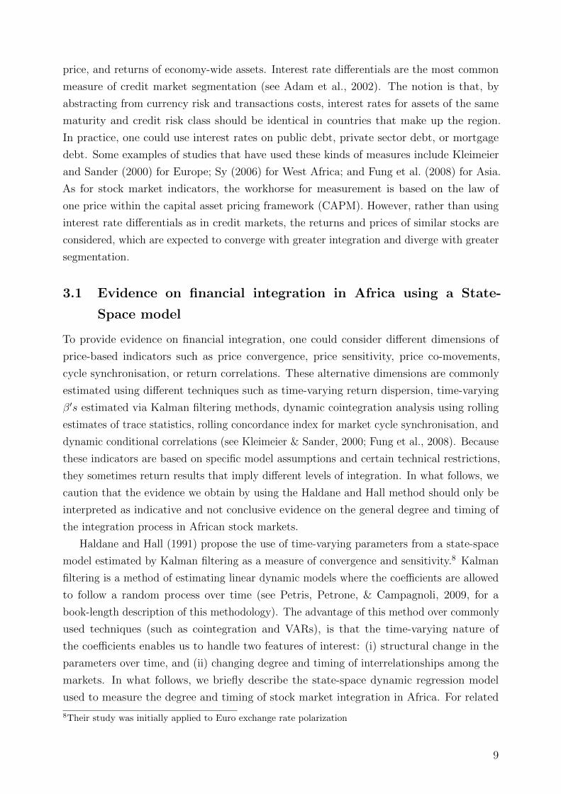
capitalization of the US equity market. In Figure 1 and Figure 2, we present the estimated

time-varying parameters (βi,t) of the model for the case where we use a weighted regional

index as the dominant market (Figure 1) and the case where we use the South African

stock market as the dominant regional market (Figure 2). Data on average annual market

value of outstanding shares for selected countries between 1990 and 2014 are retrieved from

the Standard and Poor’s (S & P) database. The selected stock markets include Botswana,

Ghana, Kenya, Namibia, Nigeria, South Africa, Swaziland, Tanzania and Zambia. The

criteria for including countries in the sample is the availability of stock market data for a

reasonable length of time.

The interpretation of the time-varying parameter (βi,t) is somewhat intuitive. When the

equity market of country i and the regional dominant market R are converging over time,

i.e., limt→∞

E(XR,t−Xi,t) = 0, then we would expect the value of beta to approach zero; that is,

limt→∞

βi,t = 0. Conversely, if country i’s market is converging to the global dominant market

(here the US market), we would expect βi,t to approach one. Therefore, in this model, the

tendency for βi,t to move towards zero indicates sensitivity of the individual market to the

influence of the regional market, which is interpreted as regional integration; whereas, βi,t

values that are leaning towards one indicate sensitivity to the global market, and, hence, can

be interpreted as financial globalization.10 Negative values of βi,t indicate that the domestic

market diverges both from regional and global markets. The role of the stochastic constant

9The formulation of Eq. (1) in levels has both economic and econometric implications. The economicimplication of using the levels is to enable an equilibrium relationship to be defined and the econometricimplication is to allow for the detection of shared stochastic trend (see Serletis & King, 1997).

10This point can be illustrated by rearranging Eq. (1) in such a way that lnXi,t is the subject. Thus, weobtain lnXi = αi,t + (1−βi,t)XR +βi,tXUS . From this expression, it can be seen that when β approacheszero, the sensitivity of the domestic stock market to the global index disappears and the local marketmainly responds to changes in the regional benchmark XR.

10

Figure 1: Sensitivity and convergence of stock markets to a regional benchmark

Financial

crises-0.5

0.0

0.5

1.0

1990 1995 2000 2005 2010Years

Tim

e va

ryin

g pa

ram

eter

s

Countries:

Nigeria

Botswana

Ghana

Kenya

Namibia

Swaziland

Tanzania

Southafrica

term αi,t in Eq. (1) is to partial out all systematic influences of the differential between the

regional and individual country stock markets, leaving those resulting from changes in the

differential between the regional and global market (see Serletis & King, 1997).

In Figure 1 we observe that stock markets in six countries: Ghana, Kenya, Namibia,

Nigeria, South Africa, and Swaziland are more responsive to the regional stock market

benchmark relative to the global (or US) benchmark between 1995 and 2005. This conclusion

is informed by the estimated values of the time-varying parameters (βi,t), which are contained

within the range -0.5 to 0.5. In this framework, we interpret this result as evidence of some

degree of financial convergence and, hence, integration during the period. The values for

the stock markets of Tanzania and Botswana are closer to unity; and after 2005, the values

for Nigeria begin to lean towards unity. This pattern indicates that these stock markets

are increasingly becoming more sensitive to changes in the global stock market relative to

the regional market. The negative values obtained for Ghana, especially during the early

1990’s, indicates that the Ghanaian stock market diverged from the regional and global

markets during this period, noting that the more recent trend indicates sensitivity towards

the regional index. The impact of the financial crisis of 2007-2010, highlighted in the figures,

does not seem to change the observed pattern of the integration process in any significant

way.

In Figure 2, we repeat the analysis assuming that the South African stock market is

the dominant regional market. We observe that only the Ghanaian and Namibian stock

markets are more sensitive to the South African regional benchmark relative to the global

benchmark. Although it is not obvious why the Ghanaian and Namibian stock markets

are more sensitive to the South African stock market, one plausible explanation, at least

11

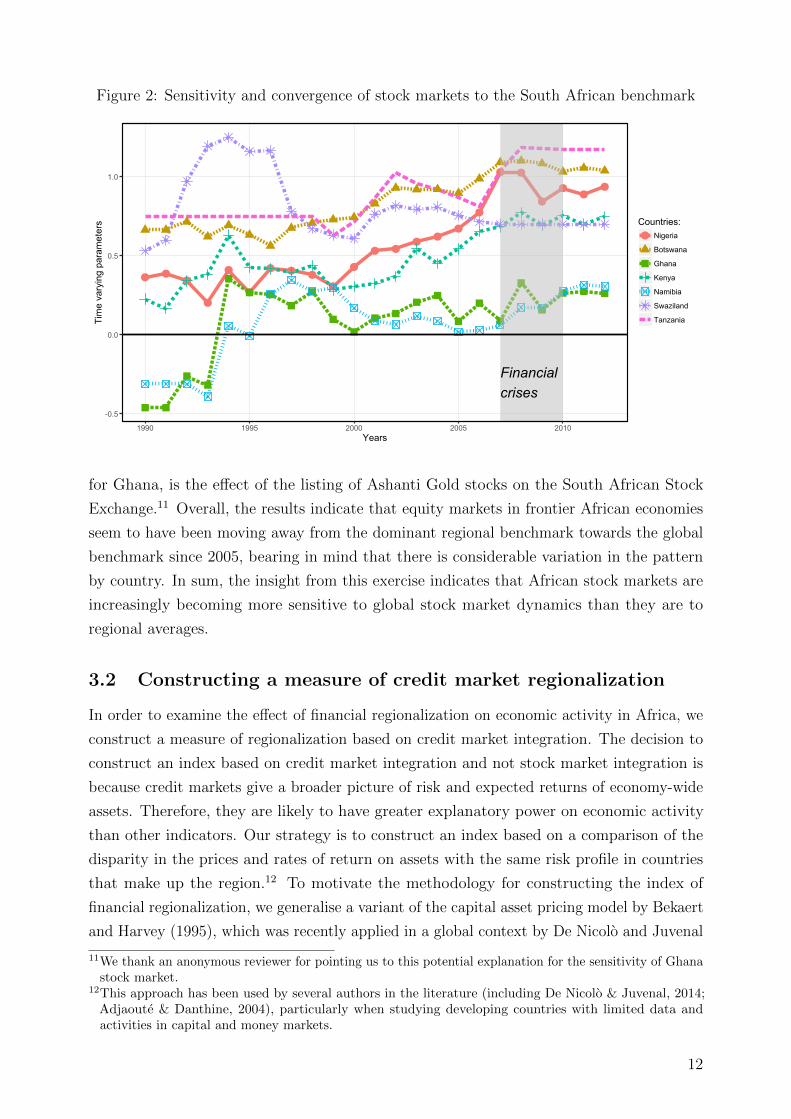
Figure 2: Sensitivity and convergence of stock markets to the South African benchmark

Financial

crises-0.5

0.0

0.5

1.0

1990 1995 2000 2005 2010Years

Tim

e va

ryin

g pa

ram

eter

s Countries:

Nigeria

Botswana

Ghana

Kenya

Namibia

Swaziland

Tanzania

for Ghana, is the effect of the listing of Ashanti Gold stocks on the South African Stock

Exchange.11 Overall, the results indicate that equity markets in frontier African economies

seem to have been moving away from the dominant regional benchmark towards the global

benchmark since 2005, bearing in mind that there is considerable variation in the pattern

by country. In sum, the insight from this exercise indicates that African stock markets are

increasingly becoming more sensitive to global stock market dynamics than they are to

regional averages.

3.2 Constructing a measure of credit market regionalization

In order to examine the effect of financial regionalization on economic activity in Africa, we

construct a measure of regionalization based on credit market integration. The decision to

construct an index based on credit market integration and not stock market integration is

because credit markets give a broader picture of risk and expected returns of economy-wide

assets. Therefore, they are likely to have greater explanatory power on economic activity

than other indicators. Our strategy is to construct an index based on a comparison of the

disparity in the prices and rates of return on assets with the same risk profile in countries

that make up the region.12 To motivate the methodology for constructing the index of

financial regionalization, we generalise a variant of the capital asset pricing model by Bekaert

and Harvey (1995), which was recently applied in a global context by De Nicolo and Juvenal

11We thank an anonymous reviewer for pointing us to this potential explanation for the sensitivity of Ghanastock market.

12This approach has been used by several authors in the literature (including De Nicolo & Juvenal, 2014;Adjaoute & Danthine, 2004), particularly when studying developing countries with limited data andactivities in capital and money markets.

12

(2014).

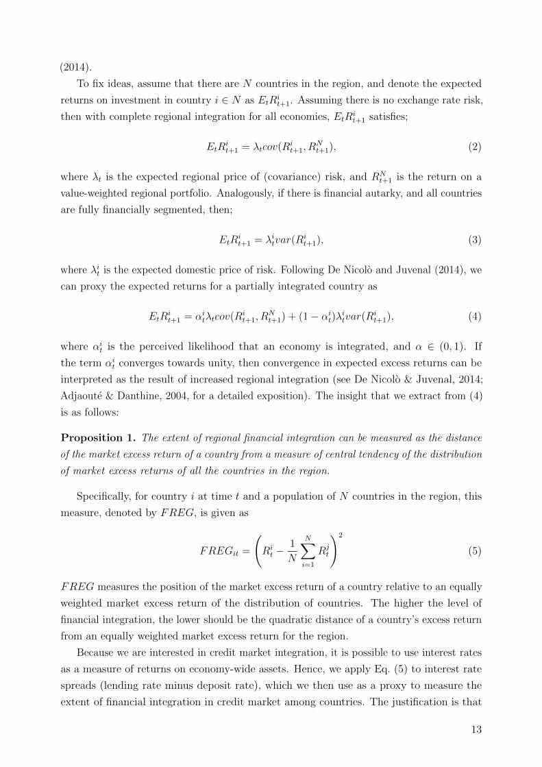
To fix ideas, assume that there are N countries in the region, and denote the expected

returns on investment in country i ∈ N as EtRit+1. Assuming there is no exchange rate risk,

then with complete regional integration for all economies, EtRit+1 satisfies;

EtRit+1 = λtcov(Ri

t+1, RNt+1), (2)

where λt is the expected regional price of (covariance) risk, and RNt+1 is the return on a

value-weighted regional portfolio. Analogously, if there is financial autarky, and all countries

are fully financially segmented, then;

EtRit+1 = λitvar(R

it+1), (3)

where λit is the expected domestic price of risk. Following De Nicolo and Juvenal (2014), we

can proxy the expected returns for a partially integrated country as

EtRit+1 = αi

tλtcov(Rit+1, R

Nt+1) + (1− αi

t)λitvar(R

it+1), (4)

where αit is the perceived likelihood that an economy is integrated, and α ∈ (0, 1). If

the term αit converges towards unity, then convergence in expected excess returns can be

interpreted as the result of increased regional integration (see De Nicolo & Juvenal, 2014;

Adjaoute & Danthine, 2004, for a detailed exposition). The insight that we extract from (4)

is as follows:

Proposition 1. The extent of regional financial integration can be measured as the distance

of the market excess return of a country from a measure of central tendency of the distribution

of market excess returns of all the countries in the region.

Specifically, for country i at time t and a population of N countries in the region, this

measure, denoted by FREG, is given as

FREGit =

(Ri

t −1

N

N∑i=1

Rjt

)2

(5)

FREG measures the position of the market excess return of a country relative to an equally

weighted market excess return of the distribution of countries. The higher the level of

financial integration, the lower should be the quadratic distance of a country’s excess return

from an equally weighted market excess return for the region.

Because we are interested in credit market integration, it is possible to use interest rates

as a measure of returns on economy-wide assets. Hence, we apply Eq. (5) to interest rate

spreads (lending rate minus deposit rate), which we then use as a proxy to measure the

extent of financial integration in credit market among countries. The justification is that

13

since bank interest rates reflect macro- and microeconomic risks and opportunities, they can

be treated as the price of risk. In that case, the convergence of these spreads to a central

tendency or benchmark over time can be interpreted as an indication that there is deepening

financial integration in the region, while divergence can be interpreted as a sign of increased

market segmentation. The closer a country’s spread is to the benchmark central value, the

more regionally integrated the country’s financial markets are and vice-versa. Summary

statistics for this index are contained in Table 3 (discussed in a later section).

4 Empirical strategy

In this section, we describe the econometric techniques that we use to characterise the

relationship between regional financial integration and economic activity in Africa. In

particular, we describe the parametric and nonparametric estimation strategies adopted.

4.1 Cross-sectional parametric analysis

The cross-sectional analysis uses data averaged over a 31-year period (1980-2011), so that

there is one observation per country per variable. By taking the average values over a that

period, we are able to abstract from business-cycle fluctuations and short-run structural

changes. This enables us to isolate the effects of these factors and focus on the long-run

growth relationship. Hence, we estimate the following heteroscedasticity-consistent growth

regression:

Yi(t−31,t) = α + λYi,31 + β1 ¯FIN i,(t−31,t) + β2 ¯FREGi,(t−31,t) + γ′Xi(t−31,t) + µit, (6)

where Y denotes economic activity, that is, Y is either economic growth or investment (capital

stock) growth. Y is the average growth rate of economic activity over the period, obtained

as Yi(t−31,t) =∑31

t=1(lnYit−lnYit−1)×100

31. FIN is a measure of financial development, FREG is

a proxy for regional financial integration, X is a vector of control variables to be described

later, and µit is the error term. The index on the regressors (t− 31, t) represents 31-year

period averages. The parameter estimate λ is a convergence term; conditional convergence in

the level of economic activity will be implied if λ < 0. The speed of convergence denoted by

ρ can be obtained by evaluation of the following expression λ = −1001−eρ3131

(see Bonfiglioli,

2008, for a detailed application).

Further, we amend Eq. (6) in such a way that enables us to investigate if there are

differences in the way that financial development and financial integration affects economic

growth under different economic, political and institutional conditions. Specifically, we

include interaction terms in the cross-sectional regression so that the estimation equation

14

becomes:

Yi(t−30,t) = α + λYi,31 + β1 ¯FIN i,(t−31,t) + β2 ¯FREGi,(t−31,t) + δ(FREGi,(t−30,t) × Z)+

γ′Xi(t−31,t) + µit, (7)

where Z is the interaction variable which could either be a measure of macroeconomic

conditions or institutional quality. When Z is a measure of institutional quality, for example,

then the interaction term enables us to assess whether financial regionalization has a stronger

effect on growth in countries with high levels of institutional quality than it does in countries

with lower levels. Specifically, we can determine this effect by evaluating the following

partial derivative

∂Y

∂FREG= β2 + δ(Z). (8)

A positive value for δ (i.e., δ > 0), will imply that financial regionalization has a greater

positive effect on growth in countries with higher levels of Z. Moreover, this interaction

term could help to examine the validity of the theoretical model by Boyd and Smith (1997),

which predicts that international financial integration would only have a positive effect on

economic performance in countries with well-developed financial systems and high levels of

institutional quality (see Edison et al., 2002).

4.2 Dynamic panel analysis by system GMM

Although the cross-sectional analysis enables us to abstract from short-run structural

dynamics and focus on long-term relationships, it is likely to produce biased and inconsistent

results due to the omission of country-fixed effects, low data frequency, and potential

endogeneity problems. For these reasons, we also examine the financial regionalization-

growth relation using a dynamic panel approach with system generalised method of moments

(GMM). Although we acknowledge that a panel IV regression approach would have been a

more appropriate route to follow, the difficult task of finding an external instrument that

satisfies both criteria of validity and informativeness has been a challenge in this literature;

hence, we have opted to follow the tradition of using an internal instrumentation strategy

based on the system GMM methodology.

The system GMM approach improves on the ordinary least squares (OLS) cross-sectional

analysis in at least three different dimensions. First, this method allows us to exploit both

the cross-section and times series nature of the data set. Second, country-specific effects are

controlled for and not subsumed in the error term when using this approach. Third, the

dynamic panel approach also controls for potential endogeneity problems in the explanatory

variables. In particular, the fact that economic activity, financial integration and financial

development could have lagged or contemporaneous dual causation implies a potential

15

violation of the endogeneity condition for standard regression analysis. We utilize the system

GMM technique developed by Holtz-Eakin, Newey, and Rosen (1988) and improved in

several dimensions by Arellano and Bond (1991), Arellano and Bover (1995), and Blundell

and Bond (1998); which has been applied in related studies such as Edison et al. (2002),

Bonfiglioli (2008), and Schularick and Steger (2010). Furthermore, by using xtabond2, a

Stata programme written independently by Roodman (2006), which enables us to use mata

syntax, we recover full control of the choice and selection of instruments.13 This method is

appropriate when we consider panel structures that contain fixed effects and idiosyncratic

errors that are heteroscedastic and correlated within but not across countries. We start

with the following growth regression

yi,t − yi,t−1 = η + τ + (α− 1)yi,t−1 + β1FINi,t + β2FREGi,t + γ′Xi,t + εi,t, (9)

where y is either the growth rate of per capita GDP, investments, or total factor productivity.

FIN is a measure of financial development, FREG is a measure of financial regionalization,

X is a vector of weakly exogenous and predetermined variables, ε is the error term, η is a

time invariant country specific effect, and τ is a deterministic time trend used to account

for period specific effects. We can simplify equation (9) in terms of the y variable, so that

yi,t = ηi + τ + αyi,t−1 + β1FINi,t + β2FREGi,t + γ′Xi,t + εi,t. (10)

To eliminate the country specific effect η, we take a first difference transformation of equation

(10) and omit the time trend for notational convenience, thus

(yi,t − yi,t−1) = α(yi,t−1 − yi,t−2) + β1(FINi,t − FINi,t−1) + β2(FREGi,t − FREGi,t−1)

+ γ′(Xi,t −Xi,t−1) + (εi,t − εi,t−1), (11)

so that by applying the difference operator, ∆, our estimation equation becomes

∆yi,t = α∆yi,t−1 + β1∆FINi,t + β2∆FREGi,t + γ′∆Xi,t + ∆εi,t. (12)

To deal with the issue of endogeneity and the fact that, by construction, the error term in Eq.

Eq. (12) is correlated with the lagged dependent variable, which compromises the consistency

of standard estimators, we introduce instrumental variables in the GMM framework (see

Arellano & Bond, 1991; Edison et al., 2002, for details). The moment conditions for the

13Roodman (2006) provides a pedagogical introduction to difference and system GMM with specificinstructions on how to use xtabond2 in Stata

16

GMM estimation are as follows.

E[yi,t−s.(εi,t − εi,t−1)] = 0; ∀s ≥ 2, t = 3 . . . T,

E[Xi,t−s.(εi,t − εi,t−1)] = 0; ∀s ≥ 2, t = 3 . . . T,(13)

where X stands for all the predetermined and weakly exogenous variables. The set of

moment conditions in Eq. (13) defines a “difference-GMM” estimator in which the lags

of the levels of the variables are used as instruments, and the country specific effects are

differenced away. This instrumentation approach is however problematic; as Blundell and

Bond (1998) have shown, this kind of instrumentation is weak, and will compromise the

asymptotic and small sample properties of the estimator through larger variances that leave

the coefficients biased. They show that the way to correct this problem is to include the

level equation in the system, and instrument the predetermined and endogenous variables

in levels with their own lagged differences. The improvement in the asymptotic and small

sample properties of this “system-GMM” estimator is then achieved through the inclusion

of additional moment conditions on the country-specific effects. That is;

E[∆yi,s.(ηi + εi,t)] = 0; ∀s ≥ 1

E[∆Xi,s.(ηi + εi,t)] = 0; ∀s ≥ 1

E[Yi,t+q.ηi] = E[Yi,t+p.ηi] = E[Xi,t+q.ηi] = E[Xi,t+p.ηi] = 0 ∀(p 6= q) ≥ 1

(14)

These moment conditions simply imply that there are no correlations between the differences

of these variables and the country specific effects, and between the future values in levels of

these variables and the country specific effects.

Because the dynamic panel data approach is an instrument-based technique, it is

important to evaluate the validity of the instruments used in the model. The estimated

coefficients are judged to be efficient and consistent if the moment conditions are satisfied,

and the instruments are valid. Instrument validity will hold if the residuals from Eq. (12)

are not second-order serially correlated. Therefore, to validate the estimates of the model,

we apply the Sargan-Hansen test of overidentifying restrictions, which is also a test of

second-order serial correlation in the residuals, and report the test statistic along with the

associated probability values.14

4.3 Nonparametric specification

The GMM specification presented above is generally robust when there are obvious concerns

about identification and potential endogeneity problems, provided the researcher has access

14Arellano and Bond (1991) show that in using this diagnostic test, estimates from the first step aremore efficient while the estimates from the second step are more robust. We, however, did not use thetwo-step method because of the long panel structure of our dataset and the fact that it requires about 546instruments to estimate the baseline regression. This requirement makes the collective set of instrumentsinvalid.

17

to valid and relevant instruments. The concern, however, is that researchers are not

often fortunate to have instruments that are valid and relevant. Moreover, the restrictive

assumptions of linearity in the parameters and normality of the error term presupposes that

the underlying relationship is linear and monotonic, an assumption that is often not suitable

for many of the ambiguous relationships in economics such as the one we are interested in,

and therefore, make them less useful for policy guidance.

To mitigate these concerns, we also consider a class of models that have less restrictive

functional specifications and are capable of handling complex problems such as nonlinearities,

complementarities, and interactions among variables in a structurally unifying manner.15

To be concrete, we consider two different estimators of nonparametric conditional mean

functions: (i) the local-constant least squares (LCLS) estimator, and (ii) the local-linear least

squares (LLLS) estimator (see Henderson & Parmeter, 2015, for a book-length treatment).

The former enables us to detect irrelevant regressors using automatically selected optimal

bandwidths, while the latter enables us to detect variables that possibly enter the relationship

with nonlinearities

The generic form of the nonparametric specification is given as

gi = m(xi) + µi, i = 1, . . . , n, (15)

where xi is the vector of all the regressors including continuous variables, unordered discreet

variables, and ordered discreet variables. m(.) is an unknown smooth growth function

(i.e., the conditional mean of g given x), and µi is the error term with no distributional

assumptions other than that it has finite second moments. The LCLS estimator for the

conditional mean in (15) at a specific point x is given by

m(x) = [i′K(x)i]−1

i′K(x)g, (16)

where g ≡ (g1, . . . , gn)′, i is an n× 1 vector of ones and K(x) is a diagonal n matrix with

kernel weighting functions and bandwidths for each variable (see Henderson et al., 2012). In

addition to governing the degree of smoothing, the bandwidths from the LCLS regression

also provides information about the relevance of the variable in the model. Hall, Li, and

Racine (2007) show that in using this estimator, when the bandwidth reaches the upper

bound, the kernel function in Eq. (16) becomes a constant, and cancels out. Hence, any

variable with bandwidths that reach the upper bound can be dropped from the model and

it would appear as though it was never even included in the model.

The second estimator, the local-linear least squares estimator, performs weighted least

squares regression around x with weights determined by a kernel function and bandwidth

15Although the nonparametric regression technique does not impose any functional restrictions on theconditional mean, nor does it impose any distributional assumptions for the error terms, it, however,requires some less restrictive assumptions such as the requirement that the function for the conditionalmean be twice continuously differentiable, and that the error term has finite variance.

18

vectors. One advantage of this method is that it nests the OLS estimator when the bandwidth

is very large. To fix ideas, consider a first-order Taylor series expansion of Eq. (15) around

x, so that16

g ≈ m(x) + (xi − x)β(xi) + εi, (17)

where β(xi) is the gradient or partial derivative of m(x) with respect to x. Thus, the LLLS

estimator of the function m(x) and partial effect β(xi) is given as

δ(x) = [X ′K(x)X]−1

X ′K(x)g, (18)

where X is an n × (qc + 1) matrix with the ith row being [1, (xci − xc)] and K(x) is a

diagonal n matrix with kernel weighting functions. The fact that we are able to obtain

fitted values for g and gradient estimates mean that we can interrogate the distribution of

the gradients to learn about potential heterogeneity in the partial effects. For the LLLS,

Hall et al. (2007) show that when the optimal bandwidth of a continuous variable reaches

the upper bound, the kernel function is a constant and cancels out from Eq. (18), so that

we are left with the familiar OLS estimator. The implication is that such a variable would

enter the model linearly. The computation of the nonparametric estimators is carried-out

using the np package in R (see Hayfield & Racine, 2008).

4.4 Data

An unbalanced panel dataset with some missing data points was collected for 17 sub-Saharan

African countries from 1980 to 2011: Benin, Botswana, Burkina Faso, Cameroon, Cote

d’Ivoire, Ethiopia, Gabon, The Gambia, Ghana, Kenya, Malawi, Nigeria, Senegal, Sierra

Leone, South Africa, Togo, and Zambia. The rationale for the sample selection is mostly

based on the availability of the required data series for a reasonable period of time. Economic

activity is proxied using three alternative variables: the growth rate of per capita GDP (Y ),

the real capital stock, and total factor productivity at 2005 constant basic prices. These

variables were obtained from the Penn World Tables (PWT) version 8.0 (Feenstra, Inklaar, &

Timmer, 2013).17 The financial regionalization variable (FREG) is obtained by calculating

the quadratic difference between a country’s interest rate spread and an equally weighted

average spread for countries in the region as explained in an earlier section. The interest

rate spread data is obtained from the IMF’s International Financial Statistics.

For financial development, we have used a bank based measure of financial depth. This

is because it is difficult to get sufficient data for alternative measures, given the nascent

state of many African stock and capital markets. Specifically, we use the ratio of domestic

16Note that this presentation is only valid for the regressors that are continuous variables.17Dataset is available at http://www.rug.nl/research/ggdc/data/penn-world-table

19

credit to the private sector over GDP as a measure of financial depth. The data is obtained

from the World Development Indicators (WDI). Inflation is measured as the growth rate

of the consumer price index and it represents a control for the prevailing macroeconomic

environment. Openness is measured as total trade to GDP ratio obtained from WDI. The

human development index variable is obtained from the PWT, and it represents the index of

human capital per person based on years of schooling—in line with Barro and Lee (2013)—

and returns to education—in line with Psacharopoulos (1994). To capture the effects of

political stability and institutional quality, we use the Polity IV project dataset from systemic

risk. This index captures the quality of democratic and autocratic authorities in governing

institutions on a spectrum of 21 points, ranging from -10 to -6 ( for autocracies), -5 to +5

(for anocracies), and +6 to +10, (for democracies).18

4.5 Descriptive statistics

Table 3 reports summary statistics for the variables used in the regressions. The values are

shown for the overall sample, the variations between countries, and the variations within

countries. The average growth rate of per capita GDP for the overall sample is 3.19, with a

standard deviation of 5.23. Most of the variation in the growth rate can be attributed to

variations in country specific growth rates over time and not from cross-sectional growth

differences, given that the standard deviation between samples is 1.47. This is an indication

that there is some homogeneity in the growth patterns of the selected economies. The

average total factor productivity in the overall sample is 1.06, with a 0.19 standard deviation

signifying technological advancements that are relatively sticky and inertial. The proxy

for financial regionalization indicates high variability, with a standard deviation of 36.56

and an average value of 20.91; the minimum value is 0.001 and the maximum is 244.29.

The between- and within-sample properties (i.e., standard deviation of 20.52 and 30.62

respectively) suggest that there is significant variability in two dimensions: the extent of

financial regionalization between countries, and the progress over time towards financial

regionalization within countries.

Financial depth is also significantly different among the countries, given a between-sample

variability of 23.43 compared to a within-sample variability of 9.82, there are significant

differences in the level of financial development among African economies. The human index

variable, polity stability, inflation, and openness variables conform to the known stylised

facts about sub-Saharan African economies.

Table 10 reports the correlation matrix of the variables used. Notice that GDP growth

is negatively correlated with our financial regionalization measure (FREG), implying a

18The Polity scheme consists of six component measures that record key qualities of executive recruitment,constraints on executive authority and political competition. It also records changes in the institutionalisedqualities of governing authority. The data is available at http://www.systemicpeace.org/inscrdata

.html

20

Table 3: Summary Statistics

Variable Grouping Mean SD Obs Min Max

GDP growth Overall 3.19 5.23 527 -28.44 28.72Between 1.47 17 1.24 7.15Within 5.03 31 -26.5 27.17

Capital stock Overall 2.64 2.83 527 -2.5 15.32Between 1.93 17 -0.95 7.41Within 2.12 31 -1.74 12.22

TFP Overall 1.06 0.19 320 0.65 2.03Between 0.11 10 0.92 1.28Within 0.16 31 0.54 1.81

Fin. Regionalization Overall 20.91 36.56 505 0.001 244.29Between 20.52 17 0.37 77.78Within 30.62 30 -56.87 214.22

Fin depth Overall 19.49 25.13 543 1.62 167.54Between 23.43 17 4.92 110.31Within 9.82 30 -35.21 76.73

Human index Overall 1.83 0.39 448 1.13 2.84Between 0.34 14 1.36 2.41Within 0.21 31 0.94 2.29

Polity stability Overall -0.61 6.19 517 -9 9Between 4.21 18 -6.18 7.25Within 4.9 31 -9.63 9.57

Inflation Overall 11.59 19.17 545 -18.58 183.31Between 12.09 18 -0.03 48.69Within 14.28 31 -34.47 146.2

Openness Overall 63.18 23.32 539 6.32 131.49Between 19.08 18 30.48 100.89Within 14.28 31 8.81 118.54

Note: The growth rate of GDP per capita and capital stock are calculated as the log-difference ofthe respective variables, multiplied by 100.

positive unconditional relationship between financial regionalization and economic growth,

although at -0.04, the correlation seems to be weak and is statistically not significant. The

unconditional correlation between GDP growth and the level of financial development is

negative and much cannot be said about this because of the low and statistically insignificant

correlation coefficient of -0.03. A negative correlation exists between the level of financial

development and our measure of financial integration (-0.08), implying that countries with

higher levels of financial development are more regionally integrated. We also observe

positive correlations between GDP growth and human capital index, polity stability, and

openness of the economy. As expected total factor productivity (TFP) is significantly

correlated with the human capital index and the polity stability index.

21

5 Empirical results and discussion

5.1 OLS cross-sectional results

For a first look at the evidence, we present the results from the cross-sectional regressions in

Table 4, successively introducing interaction terms to the baseline specification. Because

the results from this regression are only intended to provide a long-term perspective of

the relationship and because of the weakness of the cross-sectional specification already

highlighted (i.e., limited data points, omission of country-specific effects, and unaccounted

problems of endogenous causation), we prefer not to put any structural interpretation

on the results. In spite of these concerns, some interesting insights, however, emerge

from the results. For example, the results do not support the hypothesis of conditional

convergence in per capita income. Apart from the results in Model B, the sign of the

coefficient for the reference value of per capita real GDP growth in all the other models are

positive and statistically significant—a negative and significant coefficient would have implied

conditional convergence. Further, the coefficients on financial regionalization and financial

development are consistently negative, although not significant for financial regionalization

but occasionally significant for financial development. By introducing interaction terms, the

results do not change significantly, only the interaction between financial regionalization and

polity stability is statistically significant and positive, suggesting that the impact of financial

regionalization is higher in countries with higher levels of polity stability (see Model E).

This particular result does not necessarily hold in the more robust system GMM regressions,

as we will see shortly.

5.2 Dynamic panel GMM results

In Table 5, we report the results from the dynamic panel system GMM regressions. In

Models 2, 3, 4, and 6 of Table 5, the financial regionalization variable is negatively and

significantly related to growth.19 This result provides evidence that an increase in financial

regionalization, captured by a reduction in FREG, is associated with higher GDP per

capita (GDPpc) growth rates. However, because statistical and economic significance do not

always coincide, we ascertain the economic and quantitative extent of the positive effect of

financial regionalization on per capita GDP growth by multiplying the coefficient on FREG,

0.024, by the standard deviation of FREG, 36.56 (see Table 3). We do this for Model 2,

the fully specified model without interactions, and obtain 0.88, which is within close range

when using other regression equations (Models 3, 4, and 6). In more practical terms, this

result implies that a one standard deviation decline in FREG will, on average, result in an

increase in GDP growth by 0.88 of a percentage point.

The results on the financial development variable do not support the finance leading

19Most of the discussion on the results are based on the fully specified Model 2.

22

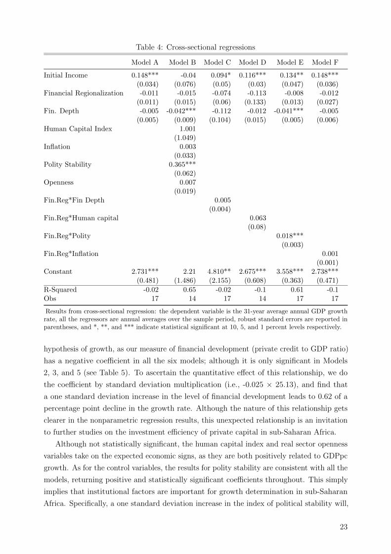
Table 4: Cross-sectional regressions

Model A Model B Model C Model D Model E Model F

Initial Income 0.148*** -0.04 0.094* 0.116*** 0.134** 0.148***(0.034) (0.076) (0.05) (0.03) (0.047) (0.036)

Financial Regionalization -0.011 -0.015 -0.074 -0.113 -0.008 -0.012(0.011) (0.015) (0.06) (0.133) (0.013) (0.027)

Fin. Depth -0.005 -0.042*** -0.112 -0.012 -0.041*** -0.005(0.005) (0.009) (0.104) (0.015) (0.005) (0.006)

Human Capital Index 1.001(1.049)

Inflation 0.003(0.033)

Polity Stability 0.365***(0.062)

Openness 0.007(0.019)

Fin.Reg*Fin Depth 0.005(0.004)

Fin.Reg*Human capital 0.063(0.08)

Fin.Reg*Polity 0.018***(0.003)

Fin.Reg*Inflation 0.001(0.001)

Constant 2.731*** 2.21 4.810** 2.675*** 3.558*** 2.738***(0.481) (1.486) (2.155) (0.608) (0.363) (0.471)

R-Squared -0.02 0.65 -0.02 -0.1 0.61 -0.1Obs 17 14 17 14 17 17

Results from cross-sectional regression: the dependent variable is the 31-year average annual GDP growthrate, all the regressors are annual averages over the sample period, robust standard errors are reported inparentheses, and *, **, and *** indicate statistical significant at 10, 5, and 1 percent levels respectively.

hypothesis of growth, as our measure of financial development (private credit to GDP ratio)

has a negative coefficient in all the six models; although it is only significant in Models

2, 3, and 5 (see Table 5). To ascertain the quantitative effect of this relationship, we do

the coefficient by standard deviation multiplication (i.e., -0.025 × 25.13), and find that

a one standard deviation increase in the level of financial development leads to 0.62 of a

percentage point decline in the growth rate. Although the nature of this relationship gets

clearer in the nonparametric regression results, this unexpected relationship is an invitation

to further studies on the investment efficiency of private capital in sub-Saharan Africa.

Although not statistically significant, the human capital index and real sector openness

variables take on the expected economic signs, as they are both positively related to GDPpc

growth. As for the control variables, the results for polity stability are consistent with all the

models, returning positive and statistically significant coefficients throughout. This simply

implies that institutional factors are important for growth determination in sub-Saharan

Africa. Specifically, a one standard deviation increase in the index of political stability will,

23

on average, lead to a 1.79 (0.29× 6.19) percentage point increase in per capita growth. The

sign on the coefficient for inflation does not conform to the theoretical expectation but, as it

is not statistically significant, it does not constitute a source of concern.

As expected, by introducing interaction terms, the observed relationships between per

capita GDP growth and financial regionalization and financial development are not altered

in any material way. From Model 3 in Table 5, the coefficient of the interaction term between

financial regionalization and financial development is positive and statistically significant

(0.031). This result can be interpreted from two perspectives depending on which variable

we hold constant as the moderating variable. If we moderate the interaction based on the

financial development variable, then the result implies that the growth-enhancing effects of

financial regionalization is greater in countries with higher levels of financial development.

On the other hand, by moderating on the financial regionalization variable, the results

imply that the growth-inhibiting effects of financial development are mitigated by financial

regionalization. This result supports some aspects of the theoretical model by Boyd and

Smith (1997), which predicts that international financial integration only have positive

effects on economic performance in countries with well-developed financial systems.

Another interesting result is the coefficient on the interaction term between financial

regionalization and polity stability (0.001). Although this coefficient is neither statistically

nor economically significant, its positive sign supports the idea that countries with higher

levels of polity stability benefit more from the growth enhancing effects of financial regional-

ization. This also goes to partially validate the result obtained from the OLS cross-sectional

regression where the interaction term is positive and statistically significant.

A careful examination of the model diagnostic test of over-identifying restrictions and

instrument validity (i.e., the Sargan test) indicates that we cannot reject the null hypothesis

that the overidentifying restrictions are valid in all the regression equations in Table 5. This

conclusion follows from the associated p-values of the Sargan test statistic. Further, the test

of second-order autocorrelation in the residuals shows that there is no second-order serial

autocorrelation in the residuals, thereby justifying the none inclusion of more lags of the

dependent variable on the right-hand side.20

In Table 6, we replicate the regressions in Table 5 with an alternate measure of economic

activity; the growth in capital stock. The results show that the nature of the relationship

between financial regionalization and investment growth in sub-Saharan Africa is somewhat

irregular, depending on the variables we control for in the regressions. In the fully specified

model with all control variables (see Model 8 of Table 6), the negative relationship between

economic activity (here, investment growth), and our proxy for financial regionalization is

preserved, indicating that countries that are more regionally integrated enjoy higher levels of

capital investments. The coefficient on the human capital index is positive and statistically

significant, implying that higher levels of educational attainment and labour participation

20For the sake of brevity, the results are not reported here, but can be made available upon request.

24

Table 5: GMM Growth Regressions: Dependent variable per capita GDP growth

Model 1 Model 2 Model 3 Model 4 Model 5 Model 6

GDPpc Growth(-1) -0.120*** -0.146*** -0.163* 0.006 -0.162*** 0.004(0.043) (0.056) (0.093) (0.054) (0.054) (0.056)

Financial Regionalization -0.014 -0.024** -0.361*** 0.513** -0.032 -0.067*(0.012) (0.012) (0.098) (0.221) (0.034) (0.04)

Fin. Depth -0.01 -0.025*** -0.705*** -0.002 -0.031*** -0.004(0.008) (0.01) (0.185) (0.011) (0.01) (0.008)

Human Capital Index 0.268 6.588***(0.678) (1.869)

Inflation 0.046 -0.029(0.049) (0.085)

Polity Stability 0.296*** 0.317***(0.047) (0.073)

Openness 0.017(0.015)

Fin.Reg*Fin. Depth 0.031***(0.008)

Fin.Reg*Human Capital -0.272**(0.117)

Fin.Reg*Polity 0.001(0.005)

Fin.Reg*Inflation 0.004*(0.002)

Constant 4.207*** 2.709* 14.784*** -9.268** 5.201*** 3.879***(0.403) (1.421) (3.168) (3.675) (0.902) (1.369)

Obs 465 334 341 341 334 341Sargan 0.63 0.06 6.8 26.09 3.34 44.05Sargan(p) 0.43 0.97 0.24 0.43 0.5 0.21Instruments 5 10 10 10 10 10

Results from GMM regression with GDP growth as dependent variable, robust standard errors are reportedin parentheses, and *, **, and *** indicate statistical significant at 10, 5, and 1 percent levels respectively.

improve the growth in the level of capital stock. Specifically, a one standard deviation

increase in the human capital index, all things being equal, will lead to a 0.31 (0.805 × 0.39)

percentage point increase in the growth of capital stock.

Further, this time, inflation assumes the expected negative sign and is statistically

significant, indicating that higher levels of macroeconomic instability reduce the potential for

capital investments by about 0.05 of a percentage point. Polity stability, having a positive

and statistically significant coefficient, implies that higher levels of polity stability positively

affects the rate of growth in the accumulation of capital stock. The only significant interaction

result in the capital stock equation is the interaction term between financial regionalization

and financial development (see Model 9 in Table 6). The positive and statistically significant

interaction coefficient of 0.004 corroborates the result in the per capita GDP regression, i.e.,

the growth-enhancing effects of financial regionalization is stronger in countries with higher

levels of financial development. It also implies that the negative effect of financial depth on

25

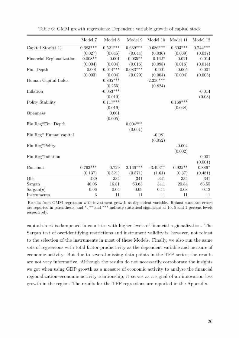
Table 6: GMM growth regressions: Dependent variable growth of capital stock

Model 7 Model 8 Model 9 Model 10 Model 11 Model 12

Capital Stock(t-1) 0.683*** 0.521*** 0.639*** 0.686*** 0.603*** 0.744***(0.027) (0.045) (0.044) (0.036) (0.039) (0.037)

Financial Regionalization 0.008** -0.001 -0.035** 0.162* 0.021 -0.014(0.004) (0.004) (0.016) (0.098) (0.016) (0.014)

Fin. Depth 0.001 -0.014*** -0.083*** -0.001 -0.005 -0.001(0.003) (0.004) (0.029) (0.004) (0.004) (0.003)

Human Capital Index 0.805*** 2.256***(0.255) (0.824)

Inflation -0.053*** -0.014(0.019) (0.03)

Polity Stability 0.117*** 0.168***(0.019) (0.038)

Openness 0.001(0.005)

Fin.Reg*Fin. Depth 0.004***(0.001)

Fin.Reg* Human capital -0.081(0.052)

Fin.Reg*Polity -0.004(0.002)

Fin.Reg*Inflation 0.001(0.001)

Constant 0.763*** 0.729 2.166*** -3.493** 0.925** 0.889*(0.137) (0.521) (0.571) (1.61) (0.37) (0.481)

Obs 439 334 341 341 334 341Sargan 46.06 16.81 63.63 34.1 20.84 63.55Sargan(p) 0.06 0.04 0.09 0.11 0.08 0.12Instruments 6 11 11 11 11 11

Results from GMM regression with investment growth as dependent variable. Robust standard errorsare reported in parenthesis, and *, ** and *** indicate statistical significant at 10, 5 and 1 percent levelsrespectively.

capital stock is dampened in countries with higher levels of financial regionalization. The

Sargan test of overidentifying restrictions and instrument validity is, however, not robust

to the selection of the instruments in most of these Models. Finally, we also run the same

sets of regressions with total factor productivity as the dependent variable and measure of

economic activity. But due to several missing data points in the TFP series, the results

are not very informative. Although the results do not necessarily corroborate the insights

we got when using GDP growth as a measure of economic activity to analyse the financial

regionalization–economic activity relationship, it serves as a signal of an innovation-less

growth in the region. The results for the TFP regressions are reported in the Appendix.

26

5.3 Nonparametric regression results

Although quite revealing, the results presented so far give us reason to suspect that some

underlying non-linearities and complementarities may be driving the nature of the effect

of financial integration on economic activity in Africa. To formally test this suspicion,

we employ Hsiao, Li, and Racine (2007)’s nonparametric and consistent test for correct

specification of parametric models to the linear panel specifications. Our choice of this

method is based on its ability to admit a mix of continuous and categorical data types,

given that our panel framework includes both countries (factor variable) and time effects

(ordered variable).21

The computed test statistic for the null hypothesis of correct model specification, Jn, is

2.59; with the associated probability value of 0.00, computed using 399 independent and

identically distributed (IID) bootstrap replications. This result indicates that the null of

correct model specification for the parametric models is rejected at the 1 percent level.

Therefore, linear parametric models, such as the ones previously reported, are likely to

return inconsistent results and so are not optimal for informing precise policy decisions. This

provides formal justification for more in-depth analysis of the growth-integration relationship

in Africa, especially in ways that account for non-linearities in the relationship; hence we

now focus on the results from the nonparametric regression analysis.

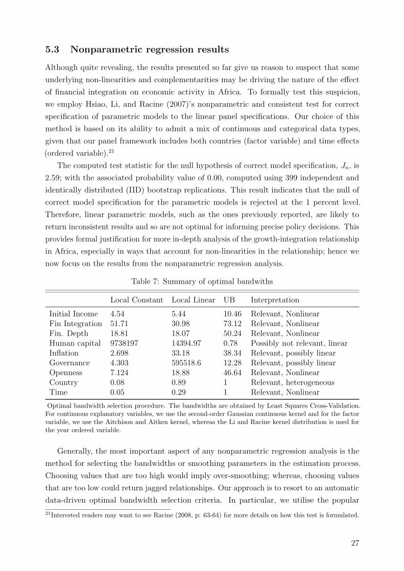
Table 7: Summary of optimal bandwiths

Local Constant Local Linear UB Interpretation

Initial Income 4.54 5.44 10.46 Relevant, NonlinearFin Integration 51.71 30.98 73.12 Relevant, NonlinearFin. Depth 18.81 18.07 50.24 Relevant, NonlinearHuman capital 9738197 14394.97 0.78 Possibly not relevant, linearInflation 2.698 33.18 38.34 Relevant, possibly linearGovernance 4.303 595518.6 12.28 Relevant, possibly linearOpenness 7.124 18.88 46.64 Relevant, NonlinearCountry 0.08 0.89 1 Relevant, heterogeneousTime 0.05 0.29 1 Relevant, Nonlinear

Optimal bandwidth selection procedure. The bandwidths are obtained by Least Squares Cross-Validation.For continuous explanatory variables, we use the second-order Gaussian continuous kernel and for the factorvariable, we use the Aitchison and Aitken kernel, whereas the Li and Racine kernel distribution is used forthe year ordered variable.

Generally, the most important aspect of any nonparametric regression analysis is the

method for selecting the bandwidths or smoothing parameters in the estimation process.

Choosing values that are too high would imply over-smoothing; whereas, choosing values

that are too low could return jagged relationships. Our approach is to resort to an automatic

data-driven optimal bandwidth selection criteria. In particular, we utilise the popular

21Interested readers may want to see Racine (2008, p: 63-64) for more details on how this test is formulated.

27

least-squares cross-validation approach within a local linear and local constant minimization

framework.

The results for the optimal bandwidth selection for each variable and the relevant

interpretations are presented in Table 7. When compared to their upper bounds (UB), these

bandwidths offer a first-round rule-of-thumb mechanism for understanding the relevance of

the regressors in the model, and the form in which they are related to the dependent variable.

In line with the recommendation in Hall et al. (2007), the upper bounds used are two times

the standard deviation of the respective variables. Furthermore, to interpret the results in

line with the analysis in Hall et al. (2007), for the local constant bandwidths, whenever a

variable’s optimal bandwidth is below its upper bound, it is interpreted as being relevant;

whereas, if it reaches or exceeds its upper bound, it is interpreted as being irrelevant.

Similarly, for the local linear optimal bandwidths, values below the upper bound indicate

that the variable is nonlinear; whereas, values above the upper bound indicate that the

variable possibly enters the regression in a linear way. From Table 7, two variables stand

out: first is the human capital index variable, with an optimal bandwidth above the upper

bound indicating that it is possibly not relevant in explaining growth; and the next is the

governance variable, with the local linear optimal bandwidth being greater than the upper

bound suggesting that it should possibly enter the regression linearly.

Table 8: Summary of partial effects and standard errors

Variable Mean Q1 Q2 Q3

Initial Income 0.3191 -0.2041 -0.0891 0.3338(0.09) (0.11) (0.06) (0.151)

Fin.Integration -0.0072 -0.0163 -0.0063 -0.0116(0.021) (0.01) (0.007) (0.021)

Fin.Depth -0.0593 -0.0726 -0.0235 0.0136(0.021) (0.027) (0.021) (0.055)

Human Capital 2.0892 0.9126 1.7719 2.4685(1.305) (0.8203) (1.099) (1.297)

Inflation -0.0118 -0.1206 0.0223 0.0634(0.041) (0.042) (0.022) (0.049)

Governance -0.0043 -0.1061 0.1477 0.1871(0.146) (0.117) (0.065) (0.059)

Openness 0.0355 -0.0103 0.0289 0.0795(0.022) (0.026) (0.017) (0.017)

The table reports the gradients, which represent the partial effects,at the mean, 25th, 50th and 75th percentiles along with the wildbootstrapped standard errors in parenthesis.

Table 8 presents the gradients. In particular, the partial effects at the mean, the 25th(Q1),

50th(Q2), and the 75th(Q3) percentiles of the estimated parameter distributions from the

local-linear nonparametric regression, along with their standard errors computed by wild

bootstrapping using Rademacher variables. One of the interesting insights we get from this

28

result is the large amount of variation we see in the partial effects at different quantiles

of the distribution for most of the variables. For example, the interquartile range of the

partial effect of financial development is 0.083 [0.013-(-0.07)]. The direction of the partial

effect also changes from being negative for lower levels of financial development to being

positive at higher levels of financial development. However, for the financial integration

variable, the variation is small, and the sign of the effect is fixed over the entire distribution

of the parameter space. The only concern is that they are not statistically significant. And

we recognise that this might be connected with the wild bootstrapping technique used to

obtain the standard errors, which may be over-controlling for heteroscedasticity, hence, a

formal test of variable significance in a nonparametric framework may be required.

Apart from the human capital index, which maintains the same sign throughout the

distribution of the parameter space, the other control variables show wide variability

between the first and third quartiles of the parameter space. The partial effects on the

human development index go to confirm the first-stage interpretation of possible linearity

of the variable based on the optimal bandwidths obtained by local linear approximations.

The results also indicate that many of the partial effects are also not statistically significant.

Although this may seem disturbing at first observation, this should not be the case, because

unlike in the parametric setting where t-values are used to judge statistical significance, here

without a formal testing of significance for each variable, we cannot tell for sure which of

the variables are relevant for predicting growth and economic activity in Africa.

Table 9: Univariate nonparametric significance tests

IID Bootstrap Wild Bootstrap

Initial Income 0.055** 0.291Fin Integration 0.027** 0.011**Fin. Depth 0.007*** 0.032**Human capital 0.265 0.298Inflation 0.045** 0.167Governance 0.025** 0.077*Openness 0.027** 0.042**

The univariate nonparametric significance test is analogous to a simplet-test, and it is based on Racine, Hart, and Li (2006); Racine (1997). IIDBootstrap indicates that the p-values are obtained by parametric bootstrapresampling from the normal distribution; whereas, Wild Bootstrap usesa wild bootstrap transformation with Rademacher variables. The latterapproach has the advantage of controlling for heteroscedasticity of unknownform on the data generating process.

Specifically, since we have estimated regression functions rather than regression parame-

ters, the standard t-testing approach often used to identify significant parameters does not

apply in this case. However, there is a sense in which the significance of the regressors could

still be tested based on the univariate nonparametric significance test for mixed data types

29

by Racine et al. (2006); Racine (1997).22 The results for this significance test are reported

in Table 9, with the associated p-values obtained using bootstrap resampling techniques,

which is appropriate given that the relevant distribution for the test statistic under the null

and alternative hypothesis are non-standard. The results in the second column of Table 9

contains p-values from IID bootstrap simulations, which assumes homoscedasticity in the

data generating process (DGP) of the variables. Using this scheme, all the regressors, save

human capital index, are statistically significant regressors in the model. However, when

we account for heteroscedasticity of unknown form in the DGP of the regressors using wild

bootstrap transformations with Rademacher variables (reported in Column 3 of Table 9),

we see that only four regressors are significant: financial integration, financial development,

governance, and openness. In what follows, we concentrate on showing how these four

variables help explain growth in Africa.

5.4 Iso-growth surface plots and contour maps

In this section, we endeavour to unpack the combined effect including potential comple-

mentarities, interactions and/or trade-offs between financial integration and other identified

significant drivers of economic activity in Africa, which were hitherto masked in the para-

metric analysis. We do this by examining the conditional mean plots of the growth surfaces

along with the financial integration variable and successive significant covariates.

In Figure 3, we plot the conditional mean surface of economic growth along with financial

integration and financial development, holding all other variables fixed at their respective

means. The plot indicates that the relationship between growth and the financial variables

are clearly non-linear. This is particularly so in the direction of financial development.

Further, the partial regression in the direction of each of the regressors does not appear to

change very much as the other predictor varies. What we see, however, is that improving

financial integration could have mild and monotonically increasing effects on growth.

Moreover, Figure 3 also shows that financial segmentation, when interacted with low

levels of financial development is consistent with negative growth rates. However, the steep

slope that characterises initial improvements in the financial sector, i.e., during the early

financial development stages, reveals the strong potential for financial development to spur

growth even when there is financial segmentation. The observed inverted-U shape along the

financial development axis also implies that there is a threshold level of financial development

that is consistent with growth in a financially segmented economy. Furthermore, there is

evidence of complementarities, as higher levels of financial development combined with more

financial integration return higher levels of growth. This revelation becomes clearer when

we examine the contour plots.

The contour maps are a cross-sectional representation of the three-dimensional (3D)

22The test hypothesis and some desirable properties of the test statistic are highlighted in Chuku, Onye,and Ajah (2017), which involves a related application.

30

Figure 3: Fitted surface of growth on financial integration and development

Financial Integration50

100150

200

Financial development

50

100

150

Grow

th

−5

0

5

−5

0

5

Figure 4: Iso-growth maps for financial integration and development

Financial Integration

Fin

anci

al D

evel

opm

ent

0 50 100 150 200

050

100

150

surface plots. They map specific points of the financial integration and financial development

variable to the same predicted level of growth; in this case, they can be referred to as iso-

growth lines. Figure 4 plots the iso-growth maps for financial integration and development

in Africa. The maps show that there are at least two scenarios consistent with the highest

attainable levels of growth around 9–9.5 percent: first is the scenario where growth is high

with moderate levels of financial development and integration, and second is the scenario

where high growth rates are attainable with some level of regional financial segmentation

31

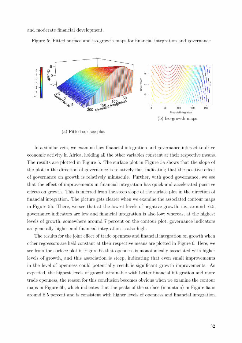
and moderate financial development.

Figure 5: Fitted surface and iso-growth maps for financial integration and governance

Financial Integration50

100150

200

Governance

−5

0

5

Gro

wth

−5

0

5

−6

−4

−2

0

2

4

6

(a) Fitted surface plot

Financial Integration

Gove

rna

nce

0 50 100 150 200

−5

05

(b) Iso-growth maps

In a similar vein, we examine how financial integration and governance interact to drive

economic activity in Africa, holding all the other variables constant at their respective means.

The results are plotted in Figure 5. The surface plot in Figure 5a shows that the slope of

the plot in the direction of governance is relatively flat, indicating that the positive effect

of governance on growth is relatively minuscule. Further, with good governance, we see

that the effect of improvements in financial integration has quick and accelerated positive

effects on growth. This is inferred from the steep slope of the surface plot in the direction of

financial integration. The picture gets clearer when we examine the associated contour maps

in Figure 5b. There, we see that at the lowest levels of negative growth, i.e., around -6.5,

governance indicators are low and financial integration is also low; whereas, at the highest

levels of growth, somewhere around 7 percent on the contour plot, governance indicators

are generally higher and financial integration is also high.

The results for the joint effect of trade openness and financial integration on growth when

other regressors are held constant at their respective means are plotted in Figure 6. Here, we

see from the surface plot in Figure 6a that openness is monotonically associated with higher

levels of growth, and this association is steep, indicating that even small improvements

in the level of openness could potentially result is significant growth improvements. As

expected, the highest levels of growth attainable with better financial integration and more

trade openness, the reason for this conclusion becomes obvious when we examine the contour

maps in Figure 6b, which indicates that the peaks of the surface (mountain) in Figure 6a is

around 8.5 percent and is consistent with higher levels of openness and financial integration.

32

Figure 6: Fitted surface and iso-growth maps for financial integration and openness

Financial Integration50

100150

200

Openness

2040

6080

100

120

Gro

wth

−5

0

5

−5

0

5

(a) Fitted surface plot

Financial Integration

Op

en

ne

ss

0 50 100 150 200

20

40

60

80

10

01

20

(b) Iso-growth maps

6 Lessons for reforms

In this section, we highlight and discuss potential policy and reform options that could

possibly enable countries in the region to exploit the growth enhancing gains from financial

regionalization, while at the same time minimising the risks associated with the process.

We discuss these options based on two criteria: first is the empirical results obtained from

the study, and second is the financial integration experiences in other regions of the world.

6.1 Lessons based on empirical results

On the degree and evolution of stock market integration in Africa, the evidence indicates

that significant progress was made between 1990 and 2005 in terms of convergence in prices

of outstanding shares. However, the convergence process seemed to have stagnated around

2005, with more contemporary evidence indicating a tilting towards financial globalisation.

Therefore, the recent trend of increased sensitivity of African stock markets to global

benchmarks could be interpreted as a first-round indicator of the heightening exposure

to contagion effects from global financial bubbles and busts. Indeed, the evidence shows

that the 2008 global financial crisis had moderate effects on selected African stock markets.

Policy reforms that seek to mitigate and cushion contagion effects from global financial

markets are necessary now than ever.

On the growth enhancing effects of financial integration, we observe that (FRED), our

proxy for financial integration, constructed based on the dispersion of a country’s interest

rate spreads from the average spread of countries in the region, is inversely related to

economic activity. Implying that tighter interest rate spreads in credit markets enhances

growth in the region. Therefore, by strengthening competition in regional banking, tighter

33

spreads could be achieved, and hence, further growth stimulated in the region.

A specific reform action along this line would be to lighten, as much as possible,

restrictions on inter-country banking establishment and operations. Further, an abatement

of the restrictions on the requirements for banks from the rest of the world (America and

Europe) to operate in Africa may be pursued to further intensify competition and hence,

achieve narrower interest rate spreads in the region. A caveat for this recommendation

is, however, instructive: because of the opaque nature of deposit money banking and the

fact that an easing of restrictions could lead to increased problems of adverse selection

and moral hazard, this policy option would have to be supported with reforms in the

ability of supervisory authorities to exercise oversight functions on banking operations across

countries.

It is also important to examine aspects of monetary policy coordination since interest

rate spreads are a function of monetary policy regimes in the different economies. To induce

convergence in interest rate spreads, monetary authorities in the region can coordinate

policies and perhaps set acceptable bands for monetary policy rates in the region. This

could also help to synchronise liquidity positions in the region since excess liquidity in some

countries could be mopped-up by banks in other countries with deficit liquidity.

6.2 Lessons based on European and Asian experience

Regional financial integration experiences from the rest of the world offer useful policy lessons

to draw from in reinforcing the momentum on financial integration in Africa. The European

Union (EU), being the pioneer and most advanced example of a relatively successful regional

financial hub, is a good place to learn from. This is particularly true in spite of the significant

economic and regulatory heterogeneity of member countries in that region, a characteristic

that is not shared by the sub-Saharan African region. We caution, however, that because of

the relatively well developed financial architecture in Europe, lessons can only be drawn

with important caveats.

The major reason that has been advanced for the relative success of the financial

integration experience in Europe is that the process was founded on consensus building,

based on a Financial Services Action Plan (FSAP) (see Sole et al., 2007). As yet, we are

not aware of any coherent region-wide financial services integration action plan for Africa.

Such a plan could be the first step in the reform process and could be facilitated through

coordination from the African Union (AU). By reviewing the EU’s Financial Services Action

Plan (FSAP), African policy makers and overseas development agencies can draw direct

lessons for reforms in Africa.

The FSAP was a five-year plan instituted in May 1999 to remove regulatory and market

barriers that limited the cross-border provision of financial services and the free flow of

capital within the EU. The distinctive feature of the plan was the process towards the

harmonisation of rules across countries in such a way that they were tight and restrictive

34

enough to ensure legal certainty, but also flexible enough to allow institutions to respond

to the dynamic nature of financial markets. The plan contained a list of 42 measures to

harmonise rules on securities, banking, insurance, mortgages, pension and all other forms

of financial transaction in the member states. By its deadline of 2004, 39 out of the 42

measures had been fully adopted by each country’s parliament. This process of coming up

with a coherent document prepared by special committees representing national governments

and stakeholders and the prompt adoption of the plan by governments would harmonise

rules for the financial sector in Africa and foster cooperation and growth within the region.

A helpful question is: how did Europe overcome its seemingly irreconcilable principles for

integration—i.e., should it be by ‘mutual recognition’, ‘competition among rules’, or simply

‘harmonisation’? The answer is not obvious because although rules had been set, most of

the financial integration goals were achieved through intra-regional trade and the means of

the market mechanism, rather than being driven by rules and command. One major factor

that helped in this direction was the volume of cross-border trade and investment which was

already in progress. Thus, the lesson for Africa is to drive the integration process through

regional trade and cross-border investments, while the institutional and legal structures

would provide the support for the market driven process.

Following the Asian crisis of 1997-98, policy makers in East Asia launched a number

of regional policy dialogues to institutionalise the interrelationships among the financial

systems that the crisis had revealed. The Chiang Mai Initiative (2000) has been the primary

initiative to strengthen existing cooperation among the members of the Association of

Southeast Asian Nations (ASEAN) including China, Japan, and the Republic of Korea.

This has helped to develop the local bond markets and complement the bank-dominated

national financial systems through the creation of two Asian Bond Funds; ABF1 and ABF2.

ABF1 is used as a channel of investment for dollar-denominated bonds issued by sovereign

and quasi-sovereign Asian borrowers; while ABF2 is used as a channel to invest in bonds

that are denominated in the local currencies. The ABF initiative practised in Asia may be

a source of inspiration for groups of regional co-operations in Africa trying to develop local

currency denominated bond markets.

7 Conclusion

Over the past three decades, there has been considerable effort towards regional finan-

cial integration in Africa. This paper endeavoured to trace the effort towards financial

regionalization in Africa by reviewing the status reports on targets set and achievements

so far. The paper estimates the degree and evolution of stock market integration using

time-varying parameters estimated by Kalman filtering techniques. Furthermore, questions

about the growth effects of regional financial integration are examined using parametric and

nonparametric regression techniques. Results from the empirical investigation are used to

35

rationalise potential reforms for enhancing the integration process in Africa.

Overall, the results show that significant progress was made towards regional financial

integration of stock markets during the 1990s and 2000s. Also, the results indicate that

improvements in the level of financial integration are associated with higher levels of economic

activity. This relationship remains valid when we control for the level of financial development,

human development index, institutional quality, and macroeconomic environment. Further,

the results show that the growth-enhancing effects of regional financial integration are

greater in countries with higher levels of financial development, although there is a threshold

beyond which they begin to diminish. When using investment growth as a measure of

economic activity, we find that countries that are more regionally financially integrated

enjoy higher levels of capital investments. The specific nature of the complementaries and

interactions are made clearer by the nonparametric regression results which neatly unpack

the complex interactions among the variables.

An aspect of the result that may be puzzling and counter-intuitive is the observation

that financial development does not necessarily lead to improvements in investment growth.

This unexpected relationship could be an invitation to further studies on the investment

efficiency of private capital investments in sub-Saharan Africa. Finally, with increasing

data availability on African stock markets, one could repeat the analysis in the paper using

returns on similarly priced investments in the capital market as an alternative measure of

financial integration in the region.

36

References

Adam, K., Jappelli, T., Menichini, A., Padula, M., & Pagano, M. (2002). Analyse,Compare, and Apply Alternative Indicators and Monitoring Methodologies to Measurethe Evolution of Capital Market Integration in the European Union. University ofSalerno, Italy.

Adjaoute, K., & Danthine, J.-P. (2004). Equity returns and integration: is Europe changing?Oxford Review of Economic Policy , 20 (4), 555–570.

Agenor, P.-R. (2003). Benefits and costs of international financial integration: theory andfacts. The World Economy , 26 (8), 1089–1118.

Ajayi, S. I., & Ndikumana, L. (2014). Capital Flight from Africa: Causes, Effects, andPolicy Issues. Oxford University Press.

Ali, A., & Imai, K. S. (2015). Crises, economic integration and growth collapses in Africancountries. Journal of African Economies , 24 (4), 471–501.

Allen, F., Otchere, I., & Senbet, L. W. (2011). African financial systems: A review. Reviewof Development Finance, 1 (2), 79–113.

Arellano, M., & Bond, S. (1991). Some tests of specification for panel data: Monte Carloevidence and an application to employment equations. The Review of EconomicStudies , 58 (2), 277–297.

Arellano, M., & Bover, O. (1995). Another look at the instrumental variable estimation oferror-components models. Journal of Econometrics , 68 (1), 29–51.

Baele, L., Ferrando, A., Hordahl, P., Krylova, E., & Monnet, C. (2004). Measuring Europeanfinancial integration. Oxford Review of Economic Policy , 20 (4), 509–530.

Barro, R. J., & Lee, J. W. (2013). A new data set of educational attainment in the world,1950–2010. Journal of Development Economics , 104 , 184–198.

Beck, T., Claessens, S., & Schmukler, S. (2013). Financial globalization and crises: Overview.The Evidence and Impact of Financial Globalization, Elsevier Inc, 1–12.

Bekaert, G., Harvey, C., & Ng, A. (2005). Market integration and contagion. Journal ofBusiness , 78 (1), 39–69.

Bekaert, G., & Harvey, C. R. (1995). Time-varying world market integration. The Journalof Finance, 50 (2), 403–444.

Blundell, R., & Bond, S. (1998). Initial conditions and moment restrictions in dynamicpanel data models. Journal of Econometrics , 87 (1), 115–143.

Bonfiglioli, A. (2008). Financial integration, productivity and capital accumulation. Journalof International Economics , 76 (2), 337–355.

Boyd, J. H., & Smith, B. D. (1997). Capital market imperfections, international creditmarkets, and nonconvergence. Journal of Economic theory , 73 (2), 335–364.

Cavoli, T., Rajan, R., & Siregar, R. (2004). A survey of financial integration in EastAsia: How far? How much further to go? Centre for International Economic Studies,University of Adelaide.

Chuku, C. (2012). The proposed eco: should West Africa proceed with a common cur-rency. Centre for the Study of African Economies (CSAE), Conference on “EconomicDevelopment in Africa” Oxford University, Oxford 18–20 March, 1–21.

Chuku, C., Onye, K., & Ajah, H. (2017). Structural and institutional determinants ofinvestment activity in Africa. In D. Seck (Ed.), Investment and Competitiveness inAfrica (pp. 25–50). Springer.

Collins, S. M. (2004). International financial integration and growth in developing countries:Issues and implications for africa. Journal of African Economies , 13 (suppl 2), ii55–ii94.

37

De Nicolo, G., & Juvenal, L. (2014). Financial integration, globalization, and real activity.Journal of Financial Stability , 10 , 65–75.

Edison, H. J., Levine, R., Ricci, L., & Sløk, T. (2002). International financial integrationand economic growth. Journal of International Money and Finance, 21 (6), 749–776.

Ekpo, A. (1994). Money, finance and economic development in ECOWAS: Theory and someevidence. West African Economic Journal , 7 (2), 83–92.

Ekpo, A., & Afangide, U. (2010). Implications of economic and financial integration formonetary management in Nigeria. West African Financial and Economic Review ,2 (2), 1–21.

Feenstra, R. C., Inklaar, R., & Timmer, M. (2013). The next generation of the Penn WorldTable (Tech. Rep.). National Bureau of Economic Research available at www.ggdc.net/pwt.

Feldstein, M., & Horioka, C. (1980). Domestic savings and international capital flows.Journal of Banking & Finance, 90 (-), 314–329.

Fung, L., Tam, C.-s., & Yu, I.-w. (2008). Assessing the integration of Asia’s equity andbond markets. BIS Paper No. 42, October .

Haldane, A. G., & Hall, S. G. (1991). Sterling’s Relationship with the Dollar and theDeutschemark: 1976-89. The Economic Journal , 436–443.

Hall, P., Li, Q., & Racine, J. S. (2007). Nonparametric estimation of regression functions inthe presence of irrelevant regressors. The Review of Economics and Statistics , 89 (4),784–789.

Hayfield, T., & Racine, J. S. (2008). Nonparametric econometrics: The np package. Journalof Statistical Software, 27 (5), 1–32.

Henderson, D. J., & Millimet, D. L. (2008). Is gravity linear? Journal of AppliedEconometrics , 23 (2), 137–172.

Henderson, D. J., Papageorgiou, C., & Parmeter, C. F. (2012). Growth empirics withoutparameters*. The Economic Journal , 122 (559), 125–154.

Henderson, D. J., & Parmeter, C. F. (2015). Applied nonparametric econometrics. CambridgeUniversity Press.

Holtz-Eakin, D., Newey, W., & Rosen, H. S. (1988). Estimating vector autoregressions withpanel data. Econometrica: Journal of the Econometric Society , 1371–1395.

Hsiao, C., Li, Q., & Racine, J. S. (2007). A consistent model specification test with mixeddiscrete and continuous data. Journal of Econometrics , 140 (2), 802–826.

IMF. (2014). Regional economic outlook: Sub-Saharan Africa, Fostering durable and inclusivegrowth. International Monetary Fund.

IMF. (2015). Pan-African Banks: opportunities and challenges for cross-border oversight.IMF–Washington D.C.

Kleimeier, S., & Sander, H. (2000). Regionalisation versus globalisation in European financialmarket integration: Evidence from co-integration analyses. Journal of Banking &Finance, 24 (6), 1005–1043.

Manning, N. (2002). Common trends and convergence? South East Asian equity markets,1988–1999. Journal of International Money and Finance, 21 (2), 183–202.

Obadan, M. I. (2006). Globalization of finance and the challenge of national financial sectordevelopment. Journal of Asian Economics , 17 (2), 316–332.

Ogunkola, E. O. (2002). The second monetary zone in West Africa and the future of asingle monetary zone in sub-Saharan Africa. Department of Economics, University ofLesotho.

Park, C.-Y., & Lee, J.-W. (2011). Financial integration in emerging Asia: Challenges andprospects. Asian Economic Policy Review , 6 (2), 176–198.

38

Petris, G., Petrone, S., & Campagnoli, P. (2009). Dynamic Linear Models. Springer.Psacharopoulos, G. (1994). Returns to investment in education: A global update. World

Development , 22 (9), 1325–1343.Racine, J. S. (1997). Consistent significance testing for nonparametric regression. Journal

of Business & Economic Statistics , 15 (3), 369–378.Racine, J. S. (2008). Nonparametric econometrics: A primer. Foundations and Trends (R)

in Econometrics , 3 (1), 1–88.Racine, J. S., Hart, J., & Li, Q. (2006). Testing the significance of categorical predictor

variables in nonparametric regression models. Econometric Reviews , 25 (4), 523–544.Roodman, D. (2006). How to do xtabond2: An introduction to difference and system GMM

in Stata. Center for Global Development working paper(103).Schularick, M., & Steger, T. M. (2010). Financial integration, investment, and economic

growth: evidence from two eras of financial globalization. The Review of Economicsand Statistics , 92 (4), 756–768.

Senbet, L. W. (1998). Globalization of African Financial Markets. In United nationsuniversity and aerc conference “africa and asia in the global economy.” tokyo, august.

Senbet, L. W. (2009). Financial sector policy reforms in the post-financial crises era: Africafocus. African Development Bank Group Working Paper Series , 1 (100), 1–.

Senbet, L. W., & Otchere, I. (2006). Financial sector reforms in Africa: perspectives onissues and policies. In Annual world bank conference on development economics 2006:Growth and integration (pp. 81–120).

Serletis, A., & King, M. (1997). Common stochastic trends and convergence of EuropeanUnion stock markets. The Manchester School , 65 (1), 44–57.

Sole, M. J., Sensenbrenner, M. G., Tahari, M. A., De Vrijer, J., Moretti, M. M., Brenner,M. P. D., & Semlali, M. A. S. (2007). Financial sector reforms and prospects forfinancial integration in maghreb countries (No. WP/07/125). International MonetaryFund.

Sy, A. N. (2006). Financial integration in the West African economic and monetary union(No. 2006-2214). International Monetary Fund.

UNECA, & AU. (2008). Assessing regional integration in Africa III: Towards monetaryand financial integration in Africa. United Nations Economic commission for Africa,Addis Ababa.

Vo, X. V. (2009). International financial integration in Asian bond markets. Research inInternational Business and Finance, 23 (1), 90–106.

Wakeman-Linn, J., & Wagh, S. (2008). Regional financial integration: Its potentialcontribution to financial sector growth and development in sub-Saharan Africa. AfricanFinance for the 21st century, Tunis, Tunisia March, 4 , 2008.

39

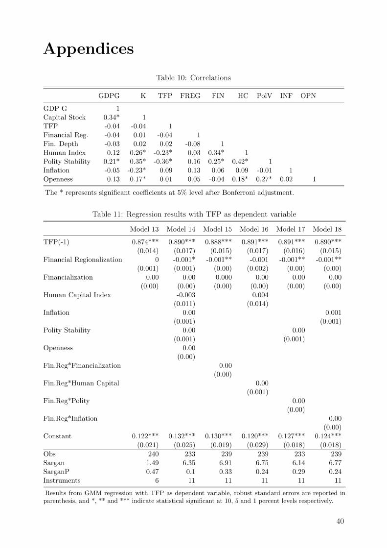
Appendices

Table 10: Correlations

GDPG K TFP FREG FIN HC PolV INF OPN

GDP G 1Capital Stock 0.34* 1TFP -0.04 -0.04 1Financial Reg. -0.04 0.01 -0.04 1Fin. Depth -0.03 0.02 0.02 -0.08 1Human Index 0.12 0.26* -0.23* 0.03 0.34* 1Polity Stability 0.21* 0.35* -0.36* 0.16 0.25* 0.42* 1Inflation -0.05 -0.23* 0.09 0.13 0.06 0.09 -0.01 1Openness 0.13 0.17* 0.01 0.05 -0.04 0.18* 0.27* 0.02 1

The * represents significant coefficients at 5% level after Bonferroni adjustment.

Table 11: Regression results with TFP as dependent variable

Model 13 Model 14 Model 15 Model 16 Model 17 Model 18

TFP(-1) 0.874*** 0.890*** 0.888*** 0.891*** 0.891*** 0.890***(0.014) (0.017) (0.015) (0.017) (0.016) (0.015)

Financial Regionalization 0 -0.001* -0.001** -0.001 -0.001** -0.001**(0.001) (0.001) (0.00) (0.002) (0.00) (0.00)

Financialization 0.00 0.00 0.000 0.00 0.00 0.00(0.00) (0.00) (0.00) (0.00) (0.00) (0.00)

Human Capital Index -0.003 0.004(0.011) (0.014)

Inflation 0.00 0.001(0.001) (0.001)

Polity Stability 0.00 0.00(0.001) (0.001)

Openness 0.00(0.00)

Fin.Reg*Financialization 0.00(0.00)

Fin.Reg*Human Capital 0.00(0.001)

Fin.Reg*Polity 0.00(0.00)

Fin.Reg*Inflation 0.00(0.00)

Constant 0.122*** 0.132*** 0.130*** 0.120*** 0.127*** 0.124***(0.021) (0.025) (0.019) (0.029) (0.018) (0.018)

Obs 240 233 239 239 233 239Sargan 1.49 6.35 6.91 6.75 6.14 6.77SarganP 0.47 0.1 0.33 0.24 0.29 0.24Instruments 6 11 11 11 11 11

Results from GMM regression with TFP as dependent variable, robust standard errors are reported inparenthesis, and *, ** and *** indicate statistical significant at 10, 5 and 1 percent levels respectively.

40