Regional Differences in Operational Efficiency of Vietnamese Ports: A Meta‐Frontier Analysis

Thi d I i l W k hThird International Workshop on Port Economics

9‐10 December, 2013 Singapore

Hong‐Oanh NguyenAustralian Maritime CollegeUniversity of TasmaniaEmail: o.nguyen@amc.edu.au.Phone: +61 3 6335 4762

Hong‐Son NghiemUniversity of QueenslandEmail: h.nghiem@uq.edu.au Phone: +61 7 3346 4785

Outline

I. Introduction

II. Literature review

III. Methodology

IV. Results

I. Introduction

Background

• Vietnam has 166 of terminals belonging to 49 sea‐ports. 

• In 2011, total throughput was 157 mil  tonnes:84% f t t l th h t t ib t d b th– 84% of total throughput was contributed by the ten largest sea‐ports. 

– 86% of containerised trade was handled by the ten largest sea‐ports. 

– The remaining sea‐ports handle only a small amount of cargo. Efficiency is critical to the ports and the local manufacturers and exporters.

Research objective

• Employs the meta‐frontier analysis method to examine the efficiency of ports within their region and with reference to the whole sector. – Ports are divided into three regions: the north– Ports are divided into three regions: the north, central and south. 

– Evaluate technological gaps between each individual regions and the sector as the whole

– Implications for port management and government

II. Literature review

Literature

• Key reviews of the port efficiency literature:– Schøyen & Odeck (2013) 

– Panayides, et al (2009)

González & Trujillo (2009)– González & Trujillo (2009)

– Cullinane & Wang (2006)

– Barros (2006)

DEA

• Early studies: Martinez‐Budria, Diaz‐Armas, Navarro‐Ibanez and Ravelo‐Mesa (1999) and Tongzon (2001).

• Martinez Budria et al (1999) applied DEA to• Martinez‐Budria et al (1999) applied DEA to study the relationship between TE and the level of “complexity”

• Barros (2006), Cullinane & Wang (2006) applied DEA to panel data to observe the trends in port efficiency. 

DEA (cont.)

• Barros & Athanassiou (2004): the scale of operation and privatisation improve TE. 

• Cullinane, et al (2006): high levels of technical efficiency are associated with scale privateefficiency are associated with scale, private‐sector participation and transhipment ports. 

• Schøyen and Odeck (2013) and de Oliveira and Cariou (2011): Scale economies exist and are important to efficiency improvement.

SFA• Schøyen Odeck (2013) found 36 studies using DEA but only 11 using SFA.

• Liu (1995) applied SFA to test if public sector ports are less efficient than private ones.

• Notteboom, et al (2000) used Bayesian stochasticNotteboom, et al (2000) used Bayesian stochastic frontier and found:

– superior performance of north European container terminals compared with southern ones

– terminals in hub ports on average be more efficient than those in feeder ports

SFA (cont.)

• Coto‐Millan, et al (2000): Spanish ports are operating on economies of scale but do not exhibit technical progress

• Cullinane & Song (2003): private participation• Cullinane & Song (2003): private participation and deregulations have a positive effect on TE

DEA vs SFA

• Only three studies (on port efficiency) compare DEA and SFA

• Cullinane, et al (2006): a high degree of correlation between the efficiency scorescorrelation between the efficiency scores obtained from the two methods

• Nguyen, et al (2011 & 2012): TE scores from both methods are useful and consistent but are different; SFA scores tend to be higher. 

Metafrontier

• Producers in different regions are generally subject to different technologies. – This effect is not accounted for in standard DEA.

• The correction is based on the metafrontier• The correction is based on the metafrontierconcept (metaproduction) defined as “the envelope of commonly conceived neoclassical production functions” 

(Hayami & Ruttan 1971, p. 82). 

Metafrontier (cont.)

• Metafrontier method is attributed to: – Battese & Rao (2002)

– Battese, et al (2004)

O’Donnell et al (2008)– O Donnell, et al (2008)

III. Methodology

Meta & group output distance functions

• A meta output distance function (DO) is defined as:

Si il l k di f i

{ })(),(,1),( xPyxMaxyxDO ∈≥= φφφ

• Similarly group k  distance function are defined as:

{ })(),(,1),( xPyxMaxyxD kO

k ∈≥= φφφ

Technological gap

• The technological gap between group frontier and meta‐frontier is measured as a ratio:

)(),(

)(),(),(

TEyxTE

DyxDyxMTR kk

Ok ==

• This ratio is interpreted as the extent to which a firm can further improve by moving from being efficient in the group (a.k.a., ‘the best’) to being efficient at the meta‐frontier (a.k.a., ‘best‐of‐the‐best’). 

),(),( yxTEyxD kO

k

Estimation of metafrontier using DEA

• Measure the distance from its input‐output structure to the meta frontier:

h φ i l λ i f

{ } NiXxyYMaxyxD iiiiO ...,,2,1 1,0 ,},{ =≥≥≥≥= φλλλφ

Where: φ is a scalar, λ is a vector of constants, X & Y are input and output matrixes of all firms, xi and yi are the input and output vectors for the ith firm. 

• The TE score is defined as 1/φ.• VRS condition:               or NIRS:∑ =1λ ∑ ≤1λ

Estimation of metafrontier using SFA

• The production function for firm i of group kfrontier model is:

• The deterministicmeta‐frontier is:

ki

ki UVk

niiii exxxfy −= );,...,,( 21 β

)(* βf

• where y* is the meta‐frontier output and β is the set of meta‐frontier parameter that satisfies the following constraint

);,...,,( 21* βniiii xxxfy =

kii xx ββ '' ≥

Estimation of metafrontier using SFA (cont.)

• The meta‐frontier is constructed by solving the following linear‐programming problem:

∑=

−N

i

kxfxf1

)];();([min βββ

• An equivalent LP is: 

s.t. lnf(x, β) ≥ lnf(x, βk)

∑=

N

ix

1'min β

β

s.t. xi’β≥ xi’βk

IV. Results

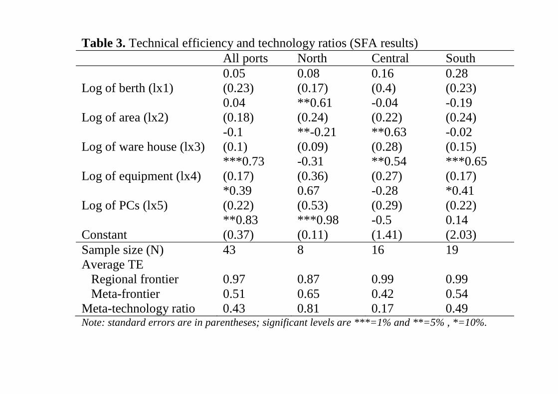
Table 3. Technical efficiency and technology ratios (SFA results) All ports North Central South

Log of berth (lx1) 0.05 (0.23)

0.08 (0.17)

0.16 (0.4)

0.28 (0.23)

Log of area (lx2) 0.04 (0.18)

**0.61 (0.24)

-0.04 (0.22)

-0.19 (0.24)

Log of ware house (lx3) -0.1 (0.1)

**-0.21 (0.09)

**0.63 (0.28)

-0.02 (0.15)

Log of equipment (lx4) ***0.73 (0.17)

-0.31 (0.36)

**0.54 (0.27)

***0.65 (0.17)

*0.39 0.67 -0.28 *0.41Log of PCs (lx5) (0.22) (0.53) (0.29) (0.22)

Constant **0.83 (0.37)

***0.98 (0.11)

-0.5 (1.41)

0.14 (2.03)

Sample size (N) 43 8 16 19 Average TE Regional frontier 0.97 0.87 0.99 0.99 Meta-frontier 0.51 0.65 0.42 0.54 Meta-technology ratio 0.43 0.81 0.17 0.49 Note: standard errors are in parentheses; significant levels are ***=1% and **=5% , *=10%.

Table 4. Technical efficiency and meta-technology ratio (DEA results) Criteria Mean Std. Dev. Min Max All ports Own technical efficiency 0.83 0.27 0.24 1.00 Meta-frontier efficiency 0.30 0.26 0.01 1.00 Meta-technology ratio 0.36 0.28 0.01 1.00 The North Own technical efficiency 0.67 0.30 0.30 1.00 Meta-frontier efficiency 0.41 0.25 0.21 1.00 Meta-technology ratio 0.65 0.27 0.27 1.00

h C lThe Central Own technical efficiency 0.81 0.31 0.24 1.00 Meta-frontier efficiency 0.19 0.17 0.01 0.62 Meta-technology ratio 0.22 0.16 0.01 0.62 The South Own technical efficiency 0.92 0.20 0.35 1.00 Meta-frontier efficiency 0.34 0.29 0.06 1.00 Meta-technology ratio 0.36 0.28 0.06 1.00

Table 5. Determinants of inter-regional technology disparities Meta-frontier technology Group frontier technology

Criteria North Central South North Central South Overall efficiency 0.41 0.19 0.34 0.41 0.68 0.67 Technical efficiency 0.59 0.39 0.65 0.67 0.81 0.92 Scale efficiency 0.73 0.66 0.62 0.65 0.84 0.74 Slack of berth 517.03 257.32 272.39 469.73 117.63 24.63 Slack of areas 91.56 111.74 275.99 92.36 2.65 3.81 Slack of ware house 21.97 3.98 16.67 15.96 1.35 0.44 Slack of equipments 533.71 133.72 488.32 608.22 130.41 0.00 Slack of PCs 26.25 1.79 45.24 26.54 4.77 0.92 Decreasing return to scale 0.13 0.00 0.11 0.13 0.06 0.26 Most efficient scale 0.13 0.00 0.11 0.13 0.38 0.32 Increasing return to scale 0.75 1.00 0.79 0.75 0.56 0.42

Influential ports: Meta‐frontier

Influential ports: Regional frontier

Thank you!