regime-switching in emerging stock market returns*6… · models, this paper ... (1996) indicate...

*The author would like to thank Simon van Norden, Narjess Boubakri, the pariticipantsof 1999 FMA and MFS meetings, Geoffery Booth, and Peter Theodossiou (managing editor)for their helpful comments and suggestions. Financial support from the Centre d’Etudes enAdministration Internationale (CETAI) is gratefully acknowledged.

(Multinational Finance Journal, 1998, vol. 2, no. 2, pp. 101–132© Multinational Finance Society, a nonprofit corporation. All rights reserved.

1

Regime-Switching in Emerging Stock MarketReturns*

Kodjovi G. AssoeEcole des Hautes Etudes Commerciales, Canada

Many emerging markets have experienced significant changes ingovernment policies and capital market reforms. These changes may lead tochanges in their return-generating processes. Based on Markov-switchingmodels, this paper investigates whether there is more than one regime in thereturn-generating processes of nine emerging markets and the specificcharacteristics of each regime. The results show very strong evidence ofregime-switching behavior in emerging stock market returns. The two regimesthrough which emerging markets evolve are different whether one takes thedomestic investors’ perspective or that of foreign investors. For foreigninvestors, changes in volatility seem to be the main characteristic of emergingmarket regimes. The implications of these findings for the stability of emergingstock markets are discussed (JEL F21, F30, G12, G15).

Keywords: emerging markets, regime-switching, international investment.

I. Introduction

Over the last two decades, the evolution of many emerging marketssuggests that the characteristics of these markets should have changed,as well as the stochastic behavior of their return-generating processes.While some emerging markets have a long history, they grewexponentially only recently in terms of market capitalization, number oflisted companies, and trading volume (Goetzmann and Jorion [1999]).

Multinational Finance Journal102

Soaring returns and good prospects for economic growth have fueled asurge of interest in emerging markets which have become moreaccessible to global investors owing to the financial liberalizationpolicies over the 80’s (Domowitz et al. [1997]; Bekaert [1995]). Themicrostructure of most emerging markets has changed markedly toaccommodate investors from industrialized countries even though a highliquidity risk, a limited number of available assets, a shortage of goodquality, and large capitalization shares remain the main differencesbetween emerging and mature markets (Richards [1996]). Furthermore,as noted by Erb et al. (1997) and Bekaert et al. (1997), the commoncharacteristic of emerging markets is the high degree of their country-risk (political risk, economic risk, and financial risk), and currencydevaluations, failed economic plans, coups, financial shocks, regulatorychanges, and capital market reforms occurred at different levels inalmost all of the emerging markets during the last decades.

Many articles have focused on the behavior of emerging marketreturns during recent years. Harvey (1995) finds that emerging marketreturns are more predictable than developed market returns and thepredictability could be induced by fundamental and operationalinefficiencies of these markets (Richards [1996]). Ghysels and Garcia(1996) indicate that the structure of the emerging markets’ returnsdistribution is unstable by rejecting the structural stability of theHarvey’s (1995) prediction model. Bekaert and Harvey (1995 and1997) show that many emerging markets are becoming more and moreintegrated into the world capital market because of the increasedimportance of world factors on emerging market expected returns.Harvey (1995) and Bekaert (1995) find that, contrary to what would beexpected from a capital asset pricing framework, higher systematic risksare associated with lower expected returns in many emerging markets.

It is widely documented that emerging stock market returns exhibithigher conditional volatility and probability of large price changes,persistence in conditional volatility, and time-varying conditionalmoments (De Santis and Imrohoroglu [1997], Bekaert et al. [1997], andTo and Assoe [1996]). Though ARCH-type models are used to providea parsimonious representation of these market return series, recentresults from De Frontnouvelle (1999) and Schaller and Van Norden(1997) suggest that the regime-switching in the underlying data-generating process could induce a non-linearity in stock market returns

103 Regime-Switching in Emerging Markets

1. In a bubble model of asset pricing, a rational risk-neutral investor may hold an assetthat is overvalued relative to its fundamentals as long as its expected return equals the returnof a non-overvalued or non-bubbly asset.

which could show up in ARCH tests. Furthermore, while To and Assoe(1996) have documented the presence of unit roots in characterizationof the emerging market return series, results from Perron (1989) indicatethat changes in regime may give the spurious impression of unit rootsin the series. Many emerging markets have displayed several largefluctuations in asset prices that are hardly explained by changes inmarket fundamentals. The existence of bubbles in emerging markets(Williamson [1993]) can result in a switching behavior in stock priceswhere an apparent deviation from fundamentals grows in one regimeand shrinks in the second regime (van Norden and Vigfusson [1998];van Norden and Schaller [1993]).1 Therefore, the main motivationbehind this article is to investigate whether there is evidence of regime-switching in emerging market return series, and the main characteristicsof each regime. There is a huge evidence of non-normalities inemerging market returns (Bekaert et al. [1998; 1997], Bekaert andHarvey [1997]) that may be explained by regime-switching. In fact, itis well known that the mixture of two normal distributions results in adistribution that is leptokurtic relative to a normal distribution since thehigh-variance distribution fattens up the tails of the low-variancedistribution. The mixture is also skewed when the means differ acrossthe two distributions. Therefore, if a given emerging market passesthrough many regimes with different mean returns and variances, thedistribution of returns in this market would be skewed and leptokurticeven if the sub-regime returns distributions are normal.

Bekaert and Harvey (1995) show that if a market is fully segmentedfrom the world equity markets, the process generating the expectedreturns in this market should be different from the one arising if thismarket were integrated to the international markets. Using a two-stateMarkov-switching model where the market can switch from asegmented state to an integrated state, they find that a number ofemerging markets have moved from segmented to integratedinternational markets. Hamilton and Susmel (1994) find that a Markov-switching model that allows discrete changes in the volatility processprovides a better statistical fit to the weekly return series of the CRSPvalue-weighted portfolio of U.S. stocks than ARCH models without


switching, a result supported by Cai (1994). De Santis and Imrohoroglu(1997) examined a regime-switching GARCH model of emergingmarket returns. They used a deterministic regime-switching model byidentifying the specific official date when each market switches fromone regime (i.e., being fully segmented) to the other (i.e., being fullyintegrated). In their model, the process of regime-switching isirreversible in the sense that when the data-generating process switchesfrom regime 1 to regime 2, it cannot come back to regime 1. In contrastto their model, Bekaert and Harvey (1995) allow markets to return to theregime of segmentation after they have been integrated. The regime-switching models presented in this article do not rely on officialliberalization dates of the emerging markets as in De Santis andImrohoroglu (1997) or postulate the influence of known global factorson the emerging market returns as in Bekaert and Harvey (1995).Instead, it is assumed that, since emerging markets have passed throughmany changes during the last decades (e.g., currency pegging or abreaking of a peg, capital market reforms, regulatory changes, politicalinstability), it is more likely that the return-generating process in thesemarkets has changed.

The purpose of this article is to analyze the behavior of the timeseries of emerging market returns and volatilities in order to investigatethe existence of different and changing regimes in these markets.Whether the means, the variances, or both the means and variancesdiffer between regimes in emerging market returns is also investigated.This is done using a set of first-order regime-switching (FORS) modelsby Gray (1997). A standard Hamilton (1989) model nested within theFORS framework is examined, where the states follow a Markovprocess with constant transition probabilities. The results show verystrong evidence of regime-switching behavior in emerging stock marketreturns whether these returns are expressed in local currencies or in U.S.dollars. The volatility switching models or the models where theregimes differ only in terms of market volatility better describe thereturn process when returns are expressed in U.S. dollars. On the otherhand, the local currency returns in many emerging markets are drawnfrom two regimes with different means and standard deviations. Thesefeatures have important implications for both international portfoliomanagers interested in investing in emerging markets and forresearchers interested in modeling returns in these markets. For


2. Results reported in this paper are mostly based on U.S. dollar returns data unlessotherwise stated. Results based on local currency data are available from the author uponrequest. Excess returns (relative to the U.S. short-term interest rate) are not used since it iswell documented that the U.S. interest rate process displays regime shifts (Garcia and Perron,[1996]; Gray, [1996]).

example, Kawakatsu and Morey (1998) raised the issue of theidentification of the liberalization dates of emerging stock markets, afactor used by De Santis and Imrohoroglu (1997). Time series modelspresented in this article can be used to identify the regime-switchingdates as the actual events dates (e.g., opening or liberalization dates).Therefore, they are complementary to the models based onfundamentals such as De Santis and Imrohoroglu (1997)’s. The ex anteprobabilities of each regime generated by the models presented hereinare of great interest for portfolio managers in forecasting the futureregime of the emerging stock markets. The rest of the paper isorganized as follows. In the next section, the data used in the study arepresented along with some descriptive statistics on emerging marketreturns. Section III presents the structure of the model and providesevidence of two regimes in the distribution of emerging market returns.The results from the estimation of regime-switching models arepresented in section IV and the conclusion follows in section V.

II. Data and Descriptive Statistics

Monthly stock market price indices from December 1975 to December1997 for nine emerging markets are used herein, namely those ofArgentina, Brazil, Chile, Greece, India, Korea, Mexico, Thailand, andZimbabwe. The data are taken from the International FinanceCorporation’s Emerging Markets Data Base (EMDB). Biases related tomarket-microstructure-induced non-randomness (e.g., thin trading, priceadjustment delays, price-discreteness-induced bias) and their impact onthe return-generating process are reduced by using monthly instead ofhigh-frequency data. Given that reliable inflation data in manyemerging markets are not available and there is a lack of reliable short-term interest rate data, total market returns expressed in local currenciesand in U.S. dollars are used herein.2

The first four moments of the distribution of each market return


3. The GMM normality test is just a Wald test for the skewness and excess kurtosiscoefficients to be jointly equal to zero. The Bera-Jarque test statistic is given by

where n is the number of observations, is the skewness, and is theBJn

= +6

252 2δ κ.1 6excess kurtosis. BJ is asymptotically distributed as chi-squared with two degrees of freedom.

series Rt are estimated in the following joint GMM-system:

,ε µ1,t tR= −

,ε µ σ22 2

,t tR= − −0 5

, and (1)ε µσ

δ3

3

3,ttR

=−

−0 5

,ε µσ4

4

4 3,ttR

k=−

− −0 5

where µ is the mean, is the standard deviation, is the skewness, isthe excess kurtosis, and t = { 1,t 2,t 3,t 4,t} represents the disturbanceswith E{ t} = 0. This system is estimated using the generalized methodof moments (GMM). There are four orthogonality conditions and fourparameters, which implies the model is exactly identified. The GMMnormality test suggested by Richardson and Smith (1993) and thestandard Bera-Jarque test of normality are performed.3

The estimated mean, standard deviation, skewness, kurtosis, andsome information on the statistical properties of dollar returns for thenine emerging markets are displayed in table 1. The mean monthlyreturns for the emerging markets ranges from .97% (Greece) to 4.76%(Argentina) in U.S. dollar terms. They are all positive and significantlydifferent from zero at the 5% level, except for Greece and Zimbabwe.The four Latin American emerging markets in the sample (Argentina,Brazil, Chile, and Mexico) have average annual (compound) returnsabove 28% over the 22-year period. Emerging market returns displayhigh volatility as measured by their monthly standard deviations thatrange from 8.01% for India to 26.74% for Argentina. The standarddeviations for five out of the nine emerging markets (i.e., Argentina,

107 R

egime-Sw

itching in Em

erging Markets

TABLE 1. Summary Statistics

Serial CorrelationsBera-

Country Mean Dev. Min Max Skewness Kurtosis 1 2 4 12 GMM Jarque

Argentina .0476* .2674* –.6495 1.7811 2.22* 9.8* .05 .07 –.04 –.09 22.45 1257.3[.8] [2.0] [6.1] [12.1] (.00) (.00)

Brazil .0213* .1616* –.5689 .5753 .51* 1.38* .04 –.03 –.08 .02 17.28 31.7[.4] [.6] [3.0] [11.9] (.00) (.00)

Chile .0264* .1060* –.2803 .6286 1.0* 3.64 .18 .22 –.03 .07 6.67 187.2[8.3] [21.3] [21.5] [51.2] (.04) (.00)

Greece .0079* .0968* –.3081 .5858 1.78* 7.88* .13 .16 –.09 –.03 14.77 811.6[3.4] [10.2] [11.4] [27.2] (.00) (.00)

India .0133* .0801* –.2438 .3527 .60* 1.68* .10 .01 .07 –.11 6.97 46.1[2.2] [2.2] [3.9] [12.1] (.03) (.00)

Korea .0097 .0938* –.3356 .4484 .50 2.64* .12 .12 .00 .11 6.53 86.1[4.2] [8.1] [8.4] [16.5] (.04) (.00)

Mexico .0215* .1240* –.5932 .3960 –.84* 3.57* .25 –.05 .01 –.02 8.58 168.7[16.1] [16.7] [17.6] [30.4] (.01) (.00)

Thailand .0104* .0854* –.3382 .3218 –.31 3.14* .11 .26 .03 .11 25.10 110.6[3.3] [21.1] [22.1] [51.6] (.00) (.00)

Zimbabwe .0104 .1012* –.3859 .4598 .02 2.08* .17 .18 .17 –.04 6.24 46.35[8.2] [14.9] [38.9] [52.9] (.04) (.00)

Note: Summary statistics relating to monthly emerging market returns. Returns are in U.S. dollars, and from January 1976 to December 1997. The means,standard deviations, skewness and kurtosis coefficients are jointly estimated via GMM for each market. 1 are serial correlations or autocorrelations of order i(i=1, 2, 4 and 12) and the values under brackets are the Ljung-Box Q-statistics up to i lags (these statistics are chi-squared distributed with i degree of freedom;critical values at the 5% level are 3.84, 5.99, 9.49 and 21.03 respectively for i=1, 2, 4 and 12). Statistics from the GMM test and the traditional Bera-Jarque testfor normality are reported with their p-values (in parentheses). * denotes statistics (the first four moments) significantly different from 0 at the 5% level.


Brazil, Chile, Mexico, and Zimbabwe) are greater than 10%. Thesample period maximum and minimum monthly returns displayed intable 1 also reveal the large swings of the emerging market returns.These returns are highly auto-correlated since the first-order auto-correlations of the Chile, Greece, India, Mexico, and Zimbabwe’smarket returns are greater than .10. Mexico displays a first-order auto-correlation of .26, the highest among the emerging markets, while SouthKorea market returns are the least auto-correlated. Positive auto-correlation may be explained by insider traders who have superiorinformation or by a group of uninformed traders who generallyextrapolate past return behavior while making their investmentdecisions.

Except for Korea, Thailand, and Zimbabwe, where the coefficientof skewness is not significantly different from zero at the 5% level, andfor Mexico, which displays a negative and statistically significantskewness, the remaining emerging markets exhibit positive andstatistically significant coefficient of skewness. Moreover, the excesskurtosis coefficients are positive and significantly different from zerofor all emerging market returns, except for Chile at the 5% level. TheGMM test for normality and the Bera-Jarque normality test statisticsunambiguously show that the distributions of the nine emerging marketreturns are non-normal. The results based on local currency returns arenot materially different.

III. Testing for a Markov Regime-Switching

The general framework of the model is presented and then restricted toa two-regime Markov switching model. Within this framework, testsfor whether there is more than one regime in the return-generatingprocesses of the emerging markets are performed.

A. General Model Setting

Let St be a discrete, latent indicator variable that identifies which of theN regimes the market is in at time t. That is, St = i, where i = 1, 2,..., N.Investors don’t know in which regime the market is and, after the fact,they can only estimate the conditional probability that the market wasin a given regime i. For example, in a two-state switching model, St =1


4. A model with time-varying transition probabilities is not used herein since the

and St = 2 may be a segmented market regime and an integrated marketregime, respectively, or a regime of surviving bubbles and a regime ofcollapsing bubbles, or a high-volatility regime and a low-volatilityregime, etc.

Changes in regime can affect the mean return, the volatility, or bothof these moments of the return distribution. To assess these effects,Hamilton’s regime-switching models are considered with constanttransition probabilities within the Gray’s (1997) FORS framework. Inother words, the state variable St follows a first-order Markovianprocess. The advantage of using this process in modeling regime-switching in emerging stock markets is that it allows investors togenerate meaningful forecasts that take into account the possibility ofthe change from one regime to another. Therefore, the ex anteprobability of being in regime i at time t conditional on the informationavailable at t–1, t–1, and denoted by is of greatp prob S ii t t t, = = −Φ 10 5importance to investors for forecasting purposes. Furthermore, thetransition or switching probabilities from one regime to another helpinvestors to assess the duration of each regime. For example, if i,i =

, the expected duration of regime i is given byprob S i S it t= =−10 5. The following general representation of the return process,1

1− −$,π i i1 6

Rt , is postulated for each emerging market:

, (2)Rt i t i t t= +µ σ ε, .

where , is the mean return and i,t is the standardE Rt t i tΦ − =10 5 µ ,

deviation. In this model, the conditional mean return and variance µ i t, σ i t,2

at time t depend on the market regime at time t (i.e., St = i) and may betime-varying. The explicit parameterization of the conditional meanprocess should depend on the data. Furthermore, the conditionalvariance can be modeled as an autoregressive process, and theconditional density function of the latent innovations, t, is assumed tobe Gaussian, that is . Finally, the most commonε σt t i tNΦ −1

20~ , ,1 6approach used in the literature is followed by considering a constantmatrix of transition or switching probabilities given by:4


eligible conditioning variables in the information set are limited. They must be independentof the contemporaneous realization of the regime (Gray [1997]). Note that this condition isnot met in most of the models presented in the literature. Diebold et al. (1995), Bekaert andHarvey (1995), and Schaller and van Norden (1997) are some examples where the switchingprobabilities are modeled as a function of some exogenous conditioning variables.

, (3)∏ =

�

!

"

$

####

π π ππ π π

π π π

1 1 1 2 1

2 1 2 2 2

1 2

, , ,

, , ,

, , ,

L

L

M M M M

L

N

N

N N N N

where . π π πi j t t i i jj

n

i jprob S j S i j i j, , ,; ; ,= = = = ∀ ≤ ≤ ∀− =∑0 5 01 11

B. Two-Regime Switching Model for Emerging Market Returns

The general model is restricted to a two-regime switching model sincethere is no a priori evidence of more than two regimes in emerging stockmarkets. To test for the regime-switching in these markets, it ispostulated that returns from a given emerging market, Rt, are drawnfrom a distribution with constant mean µ and standard deviation ifthere is no switching in regime. That is µ1 = µ2 = µ and 1 = 2 = ,so that the no-switching model or the Single-Regime Model (SRM) isstated as:

. (4)Rt t= +µ σ ε

Three alternative models are examined with switching in marketregimes. The binary regime variable, St, takes on the value of 1 whenthe market is in regime 1 and 2 when the market is in regime 2. In thefirst regime, returns are drawn from a distribution with constant meanµ1 and standard deviation 1, while, in the second regime, they aredrawn from a distribution with mean µ2 and standard deviation 2. Eachregime may be characterized by a different mean returns, a differentvolatility, or both different mean and volatility. Therefore, the firstalternative specification is the General Switching Model (GSM)


5. See Gray (1997) and Hamilton (1994) for details.

formulated as follows:

(5)R

p

p pt t

t t

t t t

Φ − =+

+ = −

%&K'K

1

1 1 1

2 2 11

µ σ ε

µ σ ε

with probabilitiy

with probability 2

,

, , .1 6

In this model, returns are assumed to be drawn from twodistributions with different means and variances. The conditionalprobability of being in regime 1 at time t, , isp prob St t t1 11, = = −Φ0 5inferred from the return series using the following recursiverepresentation:5

pg p

g p g ptt t

t t t t1 1 1

1 1 1 1

1 1 1 1 2 1 1 11, ,, ,

, , , ,

=+ −

�!

"$#

− −

− − − −

π 1 6(6)

,+ −−

+ −�!

"$#

− −

− − − −

11

12 22 1 1 1

1 1 1 1 2 1 1 1

π ,, ,

, , , ,

1 6 1 61 6

g p

g p g pt t

t t t t

where , , is the density probabilityg f R St t t1 1, = =0 5 g f R St t t2 2, = =0 5 f

function of Rt conditional on available information, and the are the transition probabilities. The termsπ i j t tprob S j S i, = = =−10 5

in brackets in equation 6 are the filter probabilities at time t – 1 andrepresent respectively and .prob St t= −1 1Φ0 5 = = −prob St t2 1Φ0 5

The second alternative is a Volatility-Switching Model (VSM),which assumes that the two regimes differ only in terms of marketvolatility, the mean return remaining the same whatever the regime, i.e.,

(7)R

p

p pt t

t t

t t t

Φ − =+

+ = −

%&K'K

1

1 1

2 2 11

µ σ ε

µ σ ε

with probabilitiy

with probability .

,

, ,1 6

The third alternative is a Mean-Switching Model (MSM), whichassumes that returns are drawn from two distributions with different

Multinational F

inance Journal112

TABLE 2. Test for Regime-switching in Emerging Markets (U.S. dollar returns)

Argentina Brazil Chile Greece India Korea Mexico Thailand Zimbabwe

A. Log likelihood

SRM –25.84 107.01 218.38 242.34 292.41 250.75 177.09 274.08 230.74GSM 47.83 127.27 240.48 292.91 313.92 270.40 208.37 302.23 242.51VSM 42.05 126.13 238.02 290.61 313.82 269.57 207.58 301.92 242.27MSM 25.57 120.11 223.24 283.04 308.15 265.22 199.38 283.95 239.57

B. Likelihood ratio: GSM, VSM, and MSM against the null of no-switching

GSM 147.35 40.51 44.19 101.14 43.02 39.29 62.56 56.30 23.53VSM 135.79 38.23 39.27 96.56 42.83 37.63 60.98 55.68 23.04MSM 102.83 26.19 9.71 81.40 31.48 28.94 44.58 19.75 17.64

C. Likelihood ratio: General Switching Model against the VSM and MSM

VSM 11.56 2.28 4.92 4.58 .19 1.67 1.58 .62 .49(p-value) (.001) (.131) (.027) (.032) (.663) (.197) (.208) (.431) (.483)MSM 44.52 14.32 34.48 19.74 11.54 10.36 17.98 36.56 5.89(p-value) (.000) (.000) (.000) (.000) (.001) (.001) (.000) (.000) (.015)

113 R

egime-Sw

itching in Em

erging Markets

TABLE 2. (Continued)

D. Ljung-Box statistics for serial correlation of the squared standardized residuals from the single regime model (SRM)

LB1 1.915 4.411 .404 .002 17.437 5.993 29.119 2.143 2.397(p-value) (.167) (.036) (.525) (.961) (.000) (.014) (.000) (.143) (.122)LB6 16.821 13.195 6.282 26.890 44.387 13.203 68.183 46.221 11.559(p-value) (.010) (.040) (.392) (.000) (.000) (.040) (.000) (.000) (.073)LB12 18.213 56.800 35.896 55.791 53.045 15.778 71.359 49.596 14.792(p-value) (.109) (.000) (.000) (.000) (.000) (.202) (.000) (.000) (.253)

Note: Panel A reports the value of the log-likelihood function for each model. Panel B reports tests of the null hypothesis of no-switching in marketreturns (SRM) against the three alternatives of regime switching (i.e., GSM, VSM, and MSM). At the 5% and 1% significance level, the critical valuesare respectively 10.34 and 13.81 for switching in mean or in volatility, and 13.52 and 17.67 for switching in both mean and standard deviation. PanelC reports standard likelihood ratio tests for the null hypothesis of VSM and MSM against the alternative of switching in both means and volatility(GSM). The test statistics are chi-squared distributed with one degree of freedom. Panel D reports the Ljung-Box statistics for serial correlation of thesquared standardized residuals from the Single Regime Model (SRM) out to i lags (LBi) with their p-values in parentheses.


means (µ1 and µ2 ) but the same volatility 1 = 2 = , i.e.,

(8)R

p

p pt t

t t

t t t

Φ − =+

+ = −

%&K'K

1

1 1

2 11

µ σ ε

µ σ ε

with probabilitiy

with probability 2

,

, , .1 6

It is important to note that, for the three alternative models, the regimeprobability pi,t varies through time while the transition probabilities aretime-invariant. Given these specifications of the nature of regime-switching in market returns, the next step is to test whether there isstatistical evidence of regime-switching in the nine emerging markets.

C. Evidence of Two Regimes in Emerging Market Returns

In this section, whether there are at least two regimes in emergingmarket return series is formally tested. Each of the three alternativeregime-switching models is tested against the null hypothesis of no-regime switching. Since the transition probabilities are not definedunder the null of no-switching, the asymptotic distributions oflikelihood ratio, Lagrange multiplier or Wald test statistics are non-standard. To determine whether there is statistically significantevidence of regime-switching, the likelihood ratio test presented byHansen (1992) is used, where the transition probabilities are treated asnuisance parameters. Garcia (1998) tabulates critical values for thisnon-standard test statistic.

With dollar return series, the likelihood ratio tests of the nullhypothesis of no-switching against the three alternative specificationsare presented in panel B of table 2. The results indicate a strongrejection of the null hypothesis of no-switching (the SRM) when thealternative is a switching in both mean and volatility (the GSM) for allnine emerging markets. In fact, the 1% critical value for the likelihoodratio statistic in this case is 17.67 while the estimated likelihood ratiosrange from 23.53 for Zimbabwe to 147.35 for Argentina. The tests alsoreject the null of no-switching when switching in volatility (VSM) is thealternative for all of the emerging markets. The 1% critical value forthe likelihood ratio statistic in this case is 13.81 while the estimatedlikelihood ratios range from 23.04 for Zimbabwe to 135.79 forArgentina. The hypothesis of no-switching in the distribution ofemerging market returns is also rejected against the alternative of

115 R

egime-Sw

itching in Em

erging Markets

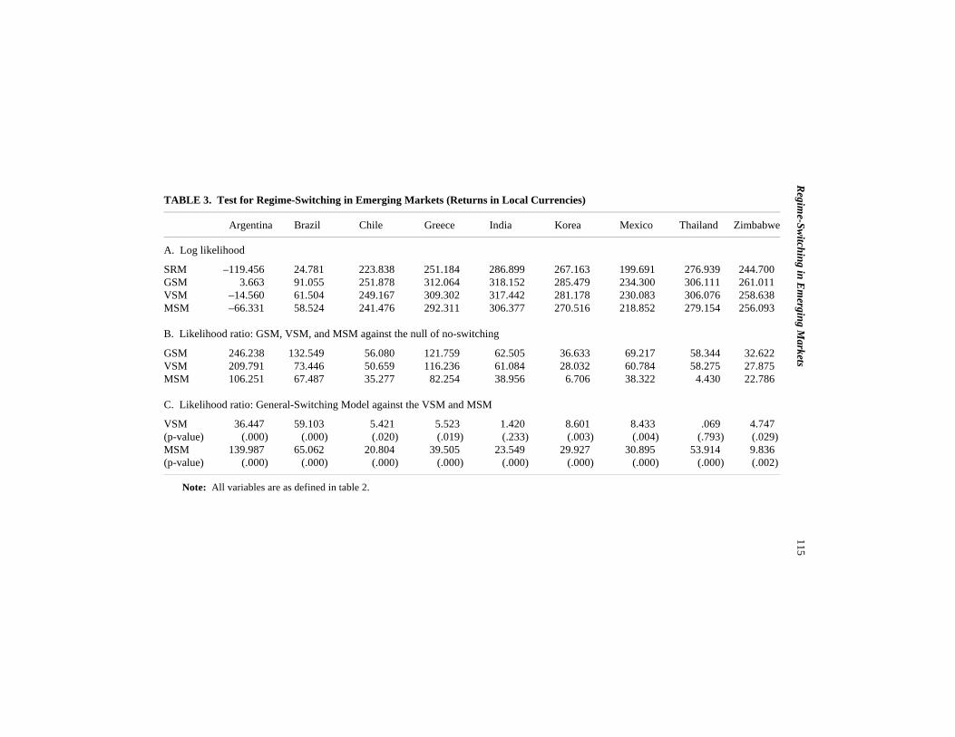
TABLE 3. Test for Regime-Switching in Emerging Markets (Returns in Local Currencies)


A. Log likelihood

SRM –119.456 24.781 223.838 251.184 286.899 267.163 199.691 276.939 244.700GSM 3.663 91.055 251.878 312.064 318.152 285.479 234.300 306.111 261.011VSM –14.560 61.504 249.167 309.302 317.442 281.178 230.083 306.076 258.638MSM –66.331 58.524 241.476 292.311 306.377 270.516 218.852 279.154 256.093

B. Likelihood ratio: GSM, VSM, and MSM against the null of no-switching

GSM 246.238 132.549 56.080 121.759 62.505 36.633 69.217 58.344 32.622VSM 209.791 73.446 50.659 116.236 61.084 28.032 60.784 58.275 27.875MSM 106.251 67.487 35.277 82.254 38.956 6.706 38.322 4.430 22.786

C. Likelihood ratio: General-Switching Model against the VSM and MSM

VSM 36.447 59.103 5.421 5.523 1.420 8.601 8.433 .069 4.747(p-value) (.000) (.000) (.020) (.019) (.233) (.003) (.004) (.793) (.029)MSM 139.987 65.062 20.804 39.505 23.549 29.927 30.895 53.914 9.836(p-value) (.000) (.000) (.000) (.000) (.000) (.000) (.000) (.000) (.002)

Note: All variables are as defined in table 2.


6. Since the results also show a strong rejection of the null of no-switching when thealternative is switching in both the mean return and the volatility (GSM) or in volatility only(VSM) for Chile, one can conclude that the regime-switching behavior of the Chilean stockmarket might be highly driven by switches in volatility rather than switches in mean returns.

switching in means (MSM) for all markets except for Chile.6 With localcurrency data, the results presented in panel B of table 3 confirm thoseobtained with dollar return series. These results show strong evidencethat, whatever the specification of the nature of switching, the null ofno-switching is rejected for almost allof the emerging markets.

The restrictions imposed by the volatility regime-switching modelwhere µ1 = µ2, and the mean regime-switching model where 1 = 2 onthe unrestricted general-switching model (µ1 ú µ2 and 1 ú 2), aretested. Panel C of table 2 (dollar return series) and table 3 (localcurrency series) reports standard likelihood ratio statistics, distributedas chi-squared with one degree of freedom, for these tests. At the 1%critical level, the results based on dollar return series show that the nullhypothesis of volatility switching (VSM) is only rejected for Argentinawhen the alternative is the GSM. The result for Argentina may bedriven at least in part by the fact that this country passed through aperiod of high turbulence (inflation, budget deficits, over-regulatedeconomy) prior to the Convertibility Act in 1991 that marked apermanent change in Argentina. Following this act, the Argentinegovernment took many other economic actions (e.g., more deregulationof the economy, privatization, liberalization, etc.) that reinforced itscommitment to price stability and economic growth. These changesresulted in more stability with more credibility and less volatility thatcommand fewer returns in the Argentine stock market. Therefore, theregime-switching in Argentina is better characterized by a simultaneousswitch in mean and volatility. The VSM is also rejected for Chile andGreece when the alternative is the GSM at the 5% level. On the otherhand, with local currency return series, the null hypothesis of volatilityswitching (VSM) is rejected for Argentina, Brazil, Chile, Greece,Korea, Mexico, and Zimbabwe (at the 5% critical level) when thealternative is the GSM. Whether the data are in local currencies or inU.S. dollars, the hypothesis of switching in mean (MSM) is rejected forall emerging stock markets when the alternative is a switch in both themean returns and the volatility (GSM).

It is very interesting to note that, at the 5% critical level, the VSM


7. The Bank of Canada Gauss procedures written by Simon van Norden, Jeff Gable, andRobert Vigfusson, as well as the Gauss code written by Stephen Gray, are used for theestimation.

hypothesis is rejected for all emerging markets but India and Thailandwhen local currency data are used and the alternative is the GSM.However, with dollar return series, the VSM is only rejected forArgentina, Chile, and Greece. These results suggest that whenemerging markets returns are subject to switches in both mean andvolatility in local currency terms (seven of the nine emerging marketsreturns are better characterized by GSM), the distribution of emergingmarket dollar returns evolves through two regimes that are differentmainly in terms of volatility (six of the nine emerging markets returnsare better characterized by VSM). These results have importantimplications for the emerging markets. Seeing that the distribution ofreturns is not the same for foreign and for domestic investors, theirrational behavior should be different. In fact, since the return-generating process is characterized by a constant expected return butcan shift periodically from low volatility to high volatility state, foreigninvestors are not fully rewarded for the risk they bear in the high-volatility regime, or they are over-rewarded in the low-volatility regime.These results confirm those of Bekaert (1995) and Harvey (1995), butonly for foreign investors and in a specific market regime. Therefore,based on foreign investors’ assessment of the ex ante probability of highvolatility regime, it may be rational to periodically observe capitalinflows and outflows from the emerging markets. Restrictions imposedby some governments on foreign ownership and trading (an example isa minimum holding period) and high transaction costs contribute to thereduction of these flows.

IV. Estimation of Switching Models in Emerging Markets

For the three regime-switching models, parameters are estimated bymaximizing the conditional log-likelihood function that is evaluatedrecursively using Hamilton’s (1994) updating formula. All models areestimated using the GAUSS MAXLIK and CML modules. An EMalgorithm is used first to get good starting values, which are then passedto MAXLIK for final convergence.7 Since the results are not materially

Multinational F

inance Journal118

TABLE 4. Parameter Estimates of the General Regime-Switching Model (GSM)

µ1 µ2 1 2 1,1 2,2 LB1 LB6 LB12 LF

Argentina –.0027 .287 .1372 .5029 .923 .635 .004 1.927 4.024 47.8(.010) (.086) (.009) (.057) (.028) (.113) (.95) (.93) (.98)

Brazil .0019 .0265 .0644 .1805 .9529 .9853 .800 3.241 25.65 127.3(.009) (.013) (.007) (.008) (.042) (.011) (.37) (.78) (.01)

Chile .0139 .1007 .0838 .1676 .9883 .9470 .321 1.951 13.94 240.5(.006) (.039) (.005) (.020) (.011) (.044) (.57) (.92) (.30)

Greece –.0029 .0668 .0642 .1860 .9867 .9233 .676 4.566 21.02 292.9(.005) (.035) (.003) (.031) (.010) (.042) (.41) (.60) (.05)

India .0063 .0193 .0457 .1028 .9492 .9453 2.446 10.70 14.10 313.8(.005) (.010) (.005) (.007) (.028) (.031) (.12) (.10) (.29)

Korea –.0016 .0392 .0632 .1439 .8930 .6845 .169 1.629 5.39 270.4(.006) (.025) (.006) (.016) (.056) (.132) (.68) (.95) (.94)

119 R

egime-Sw

itching in Em

erging Markets

TABLE 4. (Continued)

Mexico -.0250 .0305 .2323 .0863 .8258 .9667 1.021 3.164 13.49 208.4(.039) (.006) (.038) (.005) (.111) (.019) (.31) (.79) (.33)

Thailand -.0059 .0145 .1517 .0591 .8687 .9649 .220 4.579 7.91 302.0(.022) (.005) (.020) (.004) (.081) (.019) (.64) (.60) (.79)

Zimbabwe -.0420 .0408 .1069 .0834 .9611 .9703 .223 9.245 12.26 242.5(.016) (.009) (.008) (.004) (.031) (.023) (.64) (.16) (.43)

Note: Rt | t–1 = µ1+ 1 t with probability of p1,t, or Rt | t–1 = µ2+ 2 t with probability of p2,t = (1 – p1,t ), where p1,t is defined by equation 6. Estimatesare based on a sample of monthly market returns reported in U.S. dollars from January 1976 to December 1997. The average duration of each regimeis (1– i,i)

–1 . LBi denotes the Ljung-Box statistic for serial correlation of the squared standardized residuals out to i lags. LF is the maximum of log-likelihood function. Standard errors (for parameter estimates) and p-values (for Ljung-Box statistics) are in parentheses.


different with local currency data, only results based on dollar returnsare reported.

A. Parameter Estimates of GSM, VSM and MSM

Table 4 presents parameter estimates of the general regime-switchingmodel (GSM) in which emerging stock market returns are assumed tobe drawn from two distributions which differ both in their means andtheir standard deviations. The regimes are characterized by µ1 < µ2. Inregime 1, the mean returns are negative for six out of the nine emergingmarkets but are not significantly different from zero except forZimbabwe. For the three other markets where the mean returns arepositive (i.e., Brazil, Chile, and India), only the Chile market showsstatistically significant mean returns in regime 1. On the other hand,mean returns in regime 2 are all positive and significantly different fromzero (at the 10% critical level) except for South Korea. It is importantto note the large difference in mean returns between the two regimes.Except for Mexico, Thailand, and Zimbabwe, where the volatility inregime 1 (low mean-returns regime) is higher than the volatility inregime 2, the estimates of 1 and 2 show that the volatility in regime 2(high mean-returns regime) is at least twice the volatility in regime 1 forthe other six emerging markets. The estimates of the transitionprobabilities show that the two regimes are quite persistent. Theaverage expected durations range from 5.7 months in Mexico to 85.5months in Chile for regime 1 and from 2.7 months in Argentina to 68months in Brazil for regime 2. Note that when Turner et al. (1989)examined U.S. stock market returns from January 1946 to December1987, they found that the average lengths of low-variance and of high-variance episodes were 97.7 months and 3.8 months, respectively.

Table 5 presents the parameter estimates of the Volatility-SwitchingModel where regimes are identified by 1 < 2. The estimates of meanreturns are all positive, except for Greece, which has a negative butinsignificant mean return. The estimates are quite different from thoseobtained in table 1, where a constant mean and standard deviation isassumed. The distribution of Argentina stock market returns clearly illustrates this point. A single-regime model reveals a monthly meanreturn of 4.76% with a standard deviation of 26.74%, while the VSMshows that the mean return is just .51% with standard deviation of13.58% in regime 1 and 56.61% in regime 2. For all emerging markets,the volatility of returns in regime 2 is about twice or even three times

121 R

egime-Sw

itching in Em

erging Markets

TABLE 5. Parameter Estimates of the Volatility Switching Model (VSM)

µ 1 2 1,1 2,2 LB1 LB6 LB12 LF

Argentina .0051 .1358 .5661 .9214 .6483 .058 2.508 3.984 42.05(.010) (.008) (.059) (.029) (.110) (.810) (.868) (.984)

Brazil .0105 .0638 .1810 .9530 .9857 1.084 3.331 24.04 26.1(.007) (.007) (.008) (.042) (.011) (.298) (.766) (.020)

Chile .0236 .0756 .1583 .9787 .9458 .602 3.974 20.979 238.0(.006) (.005) (.012) (.022) (.048) (.438) (.680) (.051)

Greece –.0007 .0641 .1971 .9869 .9261 .470 4.124 26.368 290.6(.005) (.003) (.025) (.008) (.039) (.493) (.660) (.009)

India .0128 .0467 .0957 .9895 .9910 3.658 14.102 18.846 313.8(.004) (.004) (.005) (.010) (.007) (.056) (.029) (.092)

Korea .0063 .0673 .1507 .9445 .8044 .004 .317 3.387 269.6(.005) (.005) (.019) (.035) (.097) (.951) (.999) (.992)

Mexico .0270 .0845 .2264 .9665 .8538 1.320 2.713 14.386 207.6(.006) (.005) (.028) (.019) (.086) (.25) (.844) (.277)

Thailand .0128 .0586 .1505 .9625 .8671 .332 5.207 8.348 301.9(.004) (.004) (.019) (.019) (.079) (.564) (.518) (.757)

Zimbabwe .0154 .0698 .1388 .9437 .9114 .111 5.511 11.847 242.3(.006) (.006) (.011) (.037) (.065) (.739) (.480) (.458)

Note: Rt | t–1 = µ+ 1 t with probability of p1,t, or Rt | t–1 = µ+ 2 t with probability of p2,t = (1 – p1,t ). All variables are as defined in table 4.

Multinational F

inance Journal122

TABLE 6. Parameter Estimates of the Mean Switching Model (MSM)

µ1 µ2 1,1 2,2 LB1 LB6 LB12 LF

Argentina .0128 1.0490 .1913 .9652 .0001 8.285 23.612 25.066 25.6(.013) (.045) (.006) (.012) (.000) (.004) (.000) (.015)

Brazil -.0076 .3666 .1275 .9398 .2633 .702 9.356 43.275 120.1(.010) (.057) (.005) (.023) (.118) (.402) (.155) (.000)

Chile -.0148 .0494 .1010 .9721 .9863 .430 8.771 38.105 223.2(.019) (.011) (.003) (.044) (.018) (.512) (.187) (.000)

Greece -.0034 .3755 .0728 .9728 .0931 .041 27.279 58.5 283.0(.005) (.020) (.003) (.011) (.130) (.840) (.000) (.000)

India .0017 .1952 .0656 .9645 .3911 .211 14.666 23.049 308.1(.005) (.022) (.003) (.016) (.151) (.696) (.023) (.027)

Korea -.2953 .0124 .0862 .999 .9962 .134 .837 2.102 265.2(.171) (.006) (.003) (.000) (.006) (.715) (.991) (.999)

Mexico -.3482 .0349 .1021 .4351 .9796 6.740 35.358 42.505 199.4(.031) (.007) (.004) (.184) (.010) (.009) (.000) (.000)

Thailand -.0995 .0184 .0806 .9842 .9959 5.163 19.095 21.518 284.0(.019) (.006) (.003) (.067) (.004) (.023) (.004) (.043)

Zimbabwe -.0455 .0397 .0926 .9539 .9693 1.751 10.939 14.603 239.6(.012) (.011) (.004) (.032) (.026) (.186) (.090) (.264)

Note: Rt | t–1 = µ1+ 1 t with probability of p1,t, or Rt | t–1 = µ2+ 2 t with probability of p2,t = (1 – p1,t ). All variables are as defined in table 4.


the volatility of returns in regime 1. The estimates of transitionprobabilities show that the low-volatility regime is more persistent thanthe high-volatility regime for all emerging markets except for Brazil andIndia.

The parameter estimates of the Mean-Switching Model (MSM) arepresented in table 6. Keeping the volatility constant across regimes, theresults presented in table 5 show the enormous difference in meanreturns between the two regimes. For Argentina, Brazil, Greece, andIndia, the mean returns in regime 2 are very high, but this high returnregime does not persist when it occurs. In fact, for these countries, theaverage durations for the high-return regime range from one month forArgentina to 1.6 months for India. On the other hand, the low-returnregime is very persistent for all emerging markets except for Mexico,where monthly stock returns drop from 3.49% to –34.82% when regime1 occurs. The average duration of this low- return state is 1.77 monthsfor Mexico. South Korean market returns also show the same patternas Mexico, except that the low-return regime is more persistent. Thehigh degree of persistence of the low-return regime in South Koreareflects the impact of the recent Asian crisis from the middle of 1997until the end of our sample period. It is important to recall that theMSM is rejected when the alternative is the GSM for almost all of theemerging markets.

B. Dating Regime-switching in Emerging Market Returns

In addition to the regime-switching probabilities or the probabilities ofpersistence of each regime, there are two conditional probabilities thatare very important when dealing with the Markov regime-switchingmodels. The first, called the smoothed probability, is based on theentire data set and used to access when a switch in regime has occurred,i.e. . The second, called the ex ante probability, isprob S it T= Φ0 5especially of interest for portfolio managers in forecasting the futureregime based on information that is currently available, i.e.

. The ex ante probability series are constructedprob S it t= −Φ 10 5(equation 6) when estimating parameters of each model. The Gray's(1997) recursive procedure (smoothing filter) is used to convert ex anteprobabilities to smoothed probabilities.


FIGURE 1.—(Continued)


8. The figures which illustrate the ex ante and smoothed probabilities obtained with theGSM, the VSM, and the MSM for the nine emerging markets (local currencies and U.S. dollarreturns) are available and can be obtained from the author upon request.

FIGURE 1.—Ex Ante Regime. The ex ante probability of regime 2, , is plotted based on the best fitted model for eachprob St t= −2 1Φ0 5

country, i.e., the GSM for Argentina, Chile and Greece, and the VSMfor the other markets. Tables 4-6 provide information on the returndistribution in regime 2 for each market. Results are based on U.S.dollar return series

For the nine emerging markets studied herein, the smoothedprobability closely mirrors the ex ante probability. Periods when the exante probability of a given regime is highest end with a spike in thesmoothed probability. Therefore, only the ex ante probabilities ofregime 2 for each market are reported in figure 1 using the best fittedmodel according to the LR test, that is the GSM for Argentina, Chile,and Greece and the VSM for the other markets. For many emergingmarkets, the ex ante probabilities of regime 2 with the VSM are notmaterially different from those obtained with the GSM.8 In other words,the regime-switching documented in the GSM can be primarilyattributed to the switching in volatility. This result supports ourprevious finding from the likelihood ratio tests suggesting that the VSMcannot be rejected when the GSM is the alternative for most of theemerging markets when returns are expressed in U.S. dollars.

Figure 1 shows no common patterns in the regime-switching datesamong the emerging markets. The only exception is around October 87,


9. From 1989, 100% foreign investments in most firms are possible, except for somekey sectors (e.g., the 30% limit in the banking industry).

when there was an increase in the probability of the high-volatilityregime in all the emerging markets which, until then, had been in thelow-volatility regime. Other switches from low-to high-volatility regimeseem to be more specific to each market. For example, Argentina whichexperienced a series of switches between regime 1 and 2 during the 70sand 80s with rampant inflation, chronic budget deficits, and an over-regulated economy – has been displaying a very low probability ofregime 2 (regime with high mean return and high volatility) since theConvertibility Act in 1991. For Mexico, the ex ante probability ofregime 1 (negative mean return and high volatility) was very highduring the periods 1976, 1981-1984, and 1987-1988, and in late 1994.These periods correspond to the debt crisis (1981-1984) and especiallyto collapses of the Mexican exchange rate regime: 39% devaluation ofpeso against U.S. dollar in September 1976, 47% devaluation inDecember 1982, crawling peg with several modifications of the crawlrate in 1982 and 1984, floating of the peso in the late 1987, and pesodevaluation followed by its floating in late 1994. Except for the pesodevaluation transition period (1994-1995), the Mexican stock markethas remained in a low-volatility regime since early 1989 when mostbarriers of foreign investments were removed.9 For Thailand andKorea, figure 1 shows frequent shifts from one regime to the other, anda kind of two- or three-year cycle can be observed from the distributionof the shifts in the South Korean stock market. Moreover, theprobability of high-volatility regime increases substantially in 1996 and1997 for these markets, reflecting the Asian financial crisis. It is alsointeresting to note that the regime-switching dates based on the dollarreturn series and their best-fitted models are almost always similar tothose obtained with local currency returns.

C. Diagnostic Tests

The results presented in table 2 (panel D) show that the squaredstandardized residuals from the single-regime model (SRM) are highlyserially correlated as evidenced by the highly significant Ljung-Boxstatistics. In other words, the single regime-model does a poor job ofmodeling volatility in emerging markets. The last column of table 4, 5,

Multinational F

inance Journal128

and 6 reports the Ljung-B

ox statistics for serial correlation of the

TABLE 7. Tests for Remaining ARCH Effects


A. General Regime-switching Model (GSM)

Regression 1: R2 .035 .047 .038 .071 .061 .023 .105 .084 .019Regression 2: R2 .042 .058 .092 .137 .090 .041 .172 .127 .030F-Statistic .304 .487 2.478 3.187 1.328 .782 3.372 2.052 .473Significance level .934 .818 .024 .005 .245 .585 .003 .059 .828

B. Volatility Switching Model (VSM)

Regression 1: R2 .025 .044 .047 .041 .056 .029 .102 .090 .049Regression 2: R2 .037 .056 .079 .106 .121 .046 .162 .130 .095F-Statistic .519 .530 1.448 3.029 3.081 .742 2.983 1.916 2.118Significance level .794 .785 .197 .007 .006 .616 .008 .079 .052

C. Mean Regime-switching Model (MSM)

Regression 1: R2 .000 .002 .006 .001 .071 .001 .072 .038 .023Regression 2: R2 .039 .028 .039 .133 .170 .017 .107 .071 .039F-Statistic 1.691 1.115 1.431 6.344 4.970 .678 1.633 1.480 .694Significance level .124 .354 .203 .000 .000 .668 .138 .185 .657

Note: The squared residuals from the estimation of each model are projected on the ex ante probability of regime 2 - prob(St = 2 | t-1) - and theR-squared are reported as "Regression 1: R2". Regression 2 expands the independent variables in the previous regression by including six lagged squaredresiduals. The F-statistics are computed for the joint significance of the lagged squared residuals. Results are based on U.S. dollar return series.


squared standardized residuals out to 1, 6, and 12 lags for the GSM, theVSM, and the MSM, respectively. The results show unambiguously asignificant reduction of the Ljung-Box statistics for the threespecifications of the regime-switching model. Therefore, allowingregime-switching in emerging markets returns help to capture theirstochastic volatility.

As suggested by Garcia and Perron (1996), two regressions are runto assess the presence of any remaining ARCH effects once the shifts inmean and variance have been taken into account. First, the squaredresiduals are projected on the ex ante probabilities of regime 2. Then,the independent variables in the previous regression are expanded byincluding six lagged squared residuals. The results for these regressionsfor the GSM, the VSM, and the MSM are presented in table 7, alongwith an F-statistic to test for the joint significance of the lagged squaredresiduals. The results show that, at the 1% level, the absence of anyremaining ARCH effects cannot be rejected for seven out of the nineemerging markets once the shifts in both mean and variance (GSM) aretaken into account. For Greece and Mexico, the hypothesis of theabsence of remaining ARCH effects is rejected, suggesting the need toinvestigate a kind of GARCH regime-switching model for thesemarkets. The results are about the same with the Volatility-SwitchingModel (panel B of table 7) and the Mean-Switching Model (panel C oftable 7) except that, in addition to Greece and Mexico, an absence ofremaining ARCH effects is rejected for India. The Ljung-Box statisticsreported in tables 4, 5,and 6 also reveal dynamic behavior beyond thatcaptured by the three regime-switching models, suggesting the need toincorporate additional dynamic features such as conditional mean orvariance into these models.

V. Conclusion

Harvey (1995) and Bekaert (1995) find that higher systematic risks areassociated with lower expected returns in many emerging markets.Ignoring the problems related to the estimation of systematic risks(assumptions about the market factors, domestic or international), thisarticle shows that emerging markets go through two regimes whetherthe market returns are expressed in local currencies or in U.S. dollars.


For domestic investors (returns in local currencies), the market evolvesthrough two regimes with different mean returns and standarddeviations (GSM), and the returns are proportional to the volatility.However, for foreign investors (dollar returns), each regime is differentfrom the other, mainly with respect to the market’s volatility: TheVolatility Switching Model seems to outperform the GSM. Therefore,our results suggest that there is a regime in most emerging marketswhere the expected return is not proportional to the risk taken by foreigninvestors who express their return in U.S. dollars. When the ex anteprobability of this regime is high, foreign investors would try to go outof the market. These results may explain the numerous booms andbursts in most of emerging stock markets (Williamson, 1993), the hugecapital inflows followed by a mass redemption from the emergingmarkets by foreign investors (Howell, 1993). Switching betweenregimes seems to be associated with country-specific events such asmonetary shocks and productivity switches that lead to fluctuatingconfidence in emerging stock markets. This study can be extended toinvestigate the specific fundamental variables (e.g., macro-economic,market-specific, or firm-specific variables) that can be used to predicttransitions from one regime to another. At a theoretical level, there isa need for asset pricing models that account for the stylized facts thatemerge from this article. The first-order regime-switching modelsconsidered herein do not account for all the ARCH effects in theemerging markets. For further understanding of emerging stockmarkets, a GARCH-regime-switching model should be investigatedalong with its relative performance in forecasting emerging marketvolatility compared with that of simple GARCH models.

References

Bekaert, G. 1995. Market integration and investment barriers in emergingequity markets. World Bank Economic Review 9 (1): 75-107.

Bekaert, G. and Harvey, C. R. 1995. Time-varying world market integration.Journal of Finance 50 (2): 403-444.

Bekaert, G. and Harvey, C. R. 1997. Emerging equity market volatility. Journalof Financial Economics 43 (1): 29-77.

Bekaert, G.; Erb, C. B.; Harvey C. R.; and Viskanta, T. E. 1998. Distributionalcharacteristics of emerging market returns and asset allocation. Journal of


Portfolio Management 24 (2): 101-116.Bekaert, G.; Erb, C. B.; Harvey, C. R.; and Viskanta, T. E. 1997. What matters

for emerging equity market investments, Emerging Markets Quarterly 1 (1):17-46.

Cai, J. 1994. A markov model of switching-regime ARCH. Journal of Businessand Economic Statistics 12 (3): 309-316.

De Frontenouvelle, P. 1999. Searching for the sources of ARCH behavior:Testing the mixture of distributions model. Chapter 13. In P. Rothman (ed).Nonlinear time series analysis of economic and financial data. Norwell,Mass.: Kluwer Academic Publishers.

De Santis, G., and Imrohoroglu S. 1997. Stock returns and volatility inemerging financial markets. Journal of International Money and Finance16 (4): 561-579.

Diebold, F. X.; Lee, J. H.; and Weinbach, G. C. 1995. Regime switching withtime-varying transition probabilities. In C. Hargreaves (ed). Nonstationarytime series analysis and cointegration London, England: Oxford UniversityPress.

Domowitz, I; Glen, J.; and Madhavan, A. 1997. Market segmentation and stockprices: Evidence from an emerging market. Journal of Finance 52 (3):1059-1085.

Erb, C. B.; Harvey, C. R.; Viskanta, T. E. 1997. The making of an emergingmarket. Emerging Markets Quarterly 1 (1): 14-19.

Garcia, R. 1998. Asymptotic null distribution of the likelihood ratio test inMarkov switching models. International Economic Review 39 (3): 763-788.

Garcia, R., and Perron, P. 1996. An analysis of the real interest rate underregime shifts. Review of Economics and Statistics 78 (1): 111-125.

Ghysels, E., and Garcia, R. 1996. Structural change and asset pricing inemerging markets. Working Paper. no. 34. Montreal: University ofMontreal.

Goetzmann, W., and Jorion, P. 1999. Re-emerging markets. Journal ofFinancial and Quantitative analysis 34 (1): 1-32.

Gray, S. F. 1996. Modeling the conditional distribution of interest rates as aregime-switching process. Journal of Financial Economics 42 (1): 27-62.

Gray, S. F. 1997. An Analysis of Conditional Regime-switching Models.Working Paper. Duke University: 42 pages.

Hamilton, J. D. 1989. A new approach to the economic analysis ofnonstationary time series and the business cycle. Econometrica 57 (2): 357-384.

Hamilton, J. D. 1994. Time Series Analysis. Princeton, N.J.: PrincetonUniversity Press.

Hamilton, J. D., and Susmel, R. 1994. Autoregressive conditionalheteroskedasticity and changes in regime. Journal of Econometrics 64 (1-


2): 307-333.Hansen, Bruce E., 1992. The likelihood ratio test under nonstandard conditions:

Testing the Markov switching model of GNP. Journal of AppliedEconometrics 7: S61-S82.

Harvey, C. R. 1995. Predictable risk and returns in emerging markets. Reviewof Financial Studies 8: 773-816.

Howell, M.J. 1993. Institutional investors and emerging stock markets. In S.Claessens and S. Gooptu (eds.). Portfolio investment in developingcountries Washington, D.C.: World Bank: 78-87.

Kawakatsu H., and Morey, M. R. 1998. An empirical examination of financialliberalization and the efficiency of emerging market stock prices. Journalof Financial Research (Forthcoming).

Perron, P. 1989. The great crash, the oil price shock, and the unit roothypothesis. Econometrica 57 (6): 1361-1401.

Richards, A. J., 1996. Volatility and predictability in national stock markets:How do emerging and mature markets differ? International MonetaryFund, Staff Papers 43 (3): 461-501.

Richardson, M., and Smith,T. 1993. A test for multivariate normality in stockreturns. Journal of Business 66 (2): 295-321.

Schaller, H., Van Norden, S. 1997. Regime-switching in stock market returns.Applied Financial Economics 7 (2): 177-191.

To, Minh C., and Assoe, K. G. 1996. Dynamique des relations entre lesmarchés boursiers nord-américains et les marchés en émergence. CanadianJournal of Administrative Sciences 13 (2): 132-145.

Turner, C. M.; Startz, R.; and Nelson, C.R. 1989. A Markov model ofheteroskedasticity, risk, and learning in the stock market. Journal ofFinancial Economics. 25 (1): 3-22.

Van Norden, S., and Schaller, H. 1993. The predictability of stock marketregime: Evidence from the Toronto stock exchange. Review of Economicsand Statistics 75 (3): 505-510.

Van Norden, S., and Vigfusson, R. 1998. Avoiding the pitfalls: Can regime-switching tests reliably detect bubbles? Forthcoming in P. Rothman (ed).Studies in Nonlinear Dynamics and Econometrics. Norwell, Mass.: KluwerAcademic Publishers.

Williamson, J. 1993. Issues posed by portfolio investment in emerging markets.In S. Claessens and S. Gooptu (eds). Portfolio investment in developingcountries. Washington, D.C.: World Bank: 11-17.

regime-switching in emerging stock market returns*6… · models, this paper ... (1996) indicate...

Documents