regi.tankonyvtar.hu · web viewbioinformatics laboratory: from measurement to decision support....
TRANSCRIPT

Bioinformatics laboratory: from measurement to decision support
Antal, PéterHullám, Gábor
Millinghoffer, AndrásHajós, GergelyArany, Ádám
Bolgár, BenceGézsi, AndrásSárközy, Péter
Created by XMLmind XSL-FO Converter.

Bioinformatics laboratory: from measurement to decision supportírta Antal, Péter, Hullám, Gábor, Millinghoffer, András, Hajós, Gergely, Arany, Ádám, Bolgár, Bence, Gézsi, András, és Sárközy, Péter
Publication date 2014Szerzői jog © 2014 Antal Péter, Hullám Gábor, Millinghoffer András, Hajós Gergely, Arany Ádám, Bolgár Bence, Gézsi András, Sárközy Péter
Created by XMLmind XSL-FO Converter.

TartalomBioinformatics laboratory: from measurement to decision support ..................................................... 1
1. 1 Biobanks. Laboratory Information Management Systems .................................................. 11.1. 1.1 Introduction .......................................................................................................... 1
1.1.1. 1.1.1 Biobanks ............................................................................................... 11.1.2. 1.1.2 Laboratory Information Management Systems .................................... 2
1.2. 1.2 Features of a LIMS .............................................................................................. 21.2.1. 1.2.1 Key features .......................................................................................... 21.2.2. 1.2.2 Additional features ............................................................................... 3
1.3. 1.3 LIMS: a case study .............................................................................................. 41.4. 1.4 Questions ............................................................................................................. 7
2. 2 DNA recombinant measurement technology, noise and error models ................................ 82.1. Diseases and odds ratios ............................................................................................ 82.2. Simulating real-world measurement data .................................................................. 82.3. Library preparation .................................................................................................... 92.4. Adapter removal ......................................................................................................... 92.5. Quality filtering .......................................................................................................... 92.6. Alignment ................................................................................................................... 92.7. Bowtie 2 alignment .................................................................................................... 92.8. Visualizing results .................................................................................................... 102.9. Questions ................................................................................................................. 10
3. 3 The post-processing, haplotype reconstruction, and imputation of genetic measurements 103.1. Beckman Coulter's GenomeLab SNPstream Genotyping System .......................... 103.2. Probe/Tag Technology ............................................................................................. 103.3. SNP Assay ............................................................................................................... 113.4. Control spots ............................................................................................................ 113.5. Digital image processing methods used in genotyping studies ............................... 12
3.5.1. Filtering ....................................................................................................... 123.5.2. Grid alignment ............................................................................................ 123.5.3. Segmentation ............................................................................................... 133.5.4. Noise patterns .............................................................................................. 133.5.5. Genotyping .................................................................................................. 143.5.6. Artifact suppression ..................................................................................... 14
3.6. Questions ................................................................................................................. 154. 4 Study design: from the basics to knowledge-rich extensions ........................................... 15
4.1. Introduction ............................................................................................................. 154.2. SVM-based gene prioritization ................................................................................ 164.3. Questions ................................................................................................................. 204.4. Exercises .................................................................................................................. 204.5. Problems .................................................................................................................. 20
4.5.1. 1. Selecting data sources and similarity measures ...................................... 214.5.2. 2. Prioritizing .............................................................................................. 214.5.3. 3. Interpreting the results ............................................................................ 214.5.4. 4. Enrichment analysis ................................................................................ 21
5. 5 Bioinformatical workflow systems ................................................................................... 225.1. 5.1 Constructing data and model ............................................................................. 22
5.1.1. Tasks. ........................................................................................................... 225.2. 5.2 BMLA analysis configuration files .................................................................... 22
Created by XMLmind XSL-FO Converter.

Bioinformatics laboratory: from measurement to decision support
5.3. 5.3 Running under the system HTCondor ............................................................... 235.3.1. Tasks. ........................................................................................................... 23
5.4. 5.4 Aggregation of raw results ................................................................................. 245.4.1. Tasks. ........................................................................................................... 25
5.5. 5.5 Questions ........................................................................................................... 256. 6 Standard analysis of genetic association studies lab exercise ........................................... 25
6.1. 6.1 Introduction ....................................................................................................... 266.2. 6.2 Hardy-Weinberg equilibrium analysis ............................................................... 266.3. 6.3 Standard association tests .................................................................................. 276.4. 6.4 Haplotype association analysis .......................................................................... 28
6.4.1. 6.4.1 Linkage ............................................................................................... 296.4.2. 6.4.2 Defining haplotype blocks ................................................................. 306.4.3. 6.4.3 Association tests ................................................................................. 306.4.4. 6.4.4 Permutation tests ................................................................................ 32
7. References ............................................................................................................................ 328. 7 Analyzing Gene Expression Studies ................................................................................. 32
8.1. 7.1 Introduction ....................................................................................................... 338.1.1. 7.1.1 Dataset ................................................................................................ 33
8.2. 7.2 Installation of prerequisites ............................................................................... 338.3. 7.3 Getting the data .................................................................................................. 348.4. 7.4 Quality Control Checks ..................................................................................... 348.5. 7.5 Filtering data ...................................................................................................... 358.6. 7.6 Calculating Differential Expression .................................................................. 36
9. References ............................................................................................................................ 3810. 8 Bayesian, systems-based biomarker analysis .................................................................. 39
10.1. 8.1 Introduction ..................................................................................................... 3910.2. 8.2 Questions/Reminder ........................................................................................ 4010.3. 8.3 Exercises .......................................................................................................... 4010.4. 8.4 Postprocessing and visualization of MBS posteriors ...................................... 41
10.4.1. 8.4.1 Conditional visualization of MBS posteriors over the model structure 4110.4.2. 8.4.2 The subset lattice for the visualization of MBS and k-MBS posteriors 4210.4.3. 8.4.3 The relevance tree ............................................................................ 4510.4.4. 8.4.4 The relevance interactions ................................................................ 46
11. References .......................................................................................................................... 4712. 9 Fusion and analysis of heterogeneous biological data .................................................... 47
12.1. Introduction ........................................................................................................... 4712.2. Similarity-based prioritization ............................................................................... 4812.3. Questions ............................................................................................................... 5012.4. Exercises ................................................................................................................ 5012.5. Problems ................................................................................................................ 50
12.5.1. 1. Selecting data sources and similarity measures .................................... 5012.5.2. Composing queries, prioritizing ................................................................ 5112.5.3. 3. Interpreting the results .......................................................................... 5212.5.4. 4. Enrichment analysis .............................................................................. 54
13. 10 Bayesian, causal analysis .............................................................................................. 5513.1. 10.1 Introduction ................................................................................................... 5513.2. 10.2 Questions/Reminder ...................................................................................... 5613.3. 10.3 Exercises ........................................................................................................ 5613.4. 10.4 Conditional visualization of MBG posteriors over the model structure ........ 5713.5. 10.5 Visualization of posteriors over pairwise relation using the model layout ... 57
14. References .......................................................................................................................... 57
Created by XMLmind XSL-FO Converter.

Bioinformatics laboratory: from measurement to decision support
15. 11 Knowledge engineering for decision networks ............................................................. 5715.1. 11.1 Introduction .................................................................................................... 5815.2. 11.2 Questions/Reminder ....................................................................................... 5815.3. 11.3 Steps of knowledge engineering .................................................................... 5815.4. 11.4 Exercises ........................................................................................................ 5915.5. 11.5 Bayesian network editor ................................................................................ 59
15.5.1. 11.5.1 Creating a new BN model .............................................................. 5915.5.2. 11.5.2 Opening a BN model ...................................................................... 5915.5.3. 11.5.3 Definition of variable types ............................................................ 5915.5.4. 11.5.4 Definition of variable groups ......................................................... 6015.5.5. 11.5.5 Adding and deleting random variables (chance nodes) .................. 6115.5.6. 11.5.6 Modifying the properties of a variable (chance node) ................... 6115.5.7. 11.5.7 Adding and deleting edges ............................................................. 62
15.6. 11.6 Visualization and analysis of the estimated conditional probabilities ........... 6515.7. 11.7 Basic inference in Bayesian networks ........................................................... 66
15.7.1. 11.7.1 Setting evidences and actions ......................................................... 6615.7.2. 11.7.2 Univariate distributions conditioned on evidences and actions ..... 6615.7.3. 11.7.3 Effect of further information on inference ..................................... 67
15.8. 11.8 Visualization of structural aspects of exact inference .................................... 6815.8.1. 11.8.1 Visualization of the edges (BN) ..................................................... 6815.8.2. 11.8.2 Visualization of the chordal graph ................................................. 6815.8.3. 11.8.3 Visualization of the clique tree ....................................................... 69
16. References .......................................................................................................................... 6917. 12 Adaptation and learning in decision networks .............................................................. 71
17.1. 12.1 Introduction ................................................................................................... 7117.2. 12.2 Questions/Reminder ...................................................................................... 7117.3. 12.3 Exercises ........................................................................................................ 7117.4. 12.4 Analyzing the effect of estimation bias ........................................................ 7217.5. 12.5 Sample generation ......................................................................................... 7217.6. 12.6 Learning the BN parameters from a data set ................................................. 72
17.6.1. 12.6.1 Format of data files containing observations and interventions .. . . 7217.6.2. 12.6.2 Setting the BN parameters from a data set ..................................... 72
17.7. 12.7 Structure learning .......................................................................................... 7218. References .......................................................................................................................... 7319. 13 Virtual screening with kernel methods .......................................................................... 73
19.1. 13.1 Introduction ................................................................................................... 7319.2. 13.2 Preparing the reference compound set ........................................................... 7319.3. 13.3 Preparing kernels ........................................................................................... 7519.4. 13.4 One-class prioritization .................................................................................. 7519.5. 13.5 Quantitative Structure-Activity Relationship ................................................ 7719.6. 13.6 Questions ....................................................................................................... 78
20. References .......................................................................................................................... 7821. 14 Metagenomics ............................................................................................................... 78
21.1. 14.1 Introduction ................................................................................................... 7821.2. 14.2 Preprocessing ................................................................................................. 7821.3. 14.3 Data analysis .................................................................................................. 81
21.3.1. 14.3.1 Defining Operational Taxonomic Units ......................................... 8121.3.2. 14.3.2 Alpha-diversity ............................................................................... 8221.3.3. 14.3.3 Beta-diversity ................................................................................. 84
21.4. 14.4 Questions ....................................................................................................... 8622. References .......................................................................................................................... 86
Created by XMLmind XSL-FO Converter.

Bioinformatics laboratory: from measurement to decision support
Typotex Kiadó, http://www.typotex.hu
Creative Commons NonCommercial-NoDerivs 3.0 (CC BY-NC-ND 3.0)
A szerző nevének feltüntetése mellett nem kereskedelmi céllal szabadon másolható, terjeszthető, megjelentethető és előadható, de nem módosítható.
1. 1 Biobanks. Laboratory Information Management Systems
1.1. 1.1 Introduction
1.1.1. 1.1.1 Biobanks
Biobanks are special biorepositories that store biological samples and information related to them. Biobanks are mainly used for research purposes, especially in genomics and personalized medicine.
In most genomic research studies, in order to get meaningful, statistically significant results, researchers need to perform molecular diagnostic tests on a large number of samples typically representing tens of thousands of
Created by XMLmind XSL-FO Converter.

Bioinformatics laboratory: from measurement to decision support
individuals. Therefore, to conduct these studies, biobanks are essential to store the biological samples in an intact form until enough individuals are involved in the study. In special circumstances, for example in rare diseases, this can last to tens of years. Furthermore, samples in biobanks (especially control samples without any known disease) may be used for multiple studies by multiple researchers, decreasing the sample collection time, or increasing the number of samples used in a study. This creates the potential for more successful studies by getting more sound, biologically meaningful results, or more positive, statistically significant results. Biobanks are therefore essential tools in today's bioscience.
1.1.2. 1.1.2 Laboratory Information Management Systems
A molecular diagnostic laboratory usually works with biological samples, analyzes them and creates reports about them. This workflow has many steps that an information management system can support. The software system that offers these capabilities among others (basically the whole operational landscape of the lab) is called Laboratory Information Management Systems (LIMS). With LIMS, a lot of error-prone, manual work of the technicians can be substituted with much more efficient machine work.
1.2. 1.2 Features of a LIMS
1.2.1. 1.2.1 Key features
1.2.1.1. Sample management, logging and accession
Sample management (logging and accession of samples) is a core function of a LIMS. Registering of the samples in the LIMS can be usually initiated in two different time points: (1) when the sample is received in the laboratory, at which time point it is registered in the LIMS, or (2) in advance: before the sample is taken from the individual, the LIMS generates an order for the sample, possibly by generating a sample container and sending it to the individual. The sample is created in an "unreceived" state, and when the sample container is received in the lab, the registration process continues.
The sample management service of the LIMS has to fulfill some basic features:
• Simple forms. Data forms should be as simple as they can be, supporting easy and quick data entry no matter how many samples we are logging in.
• Flexible data input. The LIMS should support the entering of all types of data, for example numeric, alphabetic, symbols, photographic etc. Optionally, derived data, e.g. user defined functions can be automatically computed while entering data.
• Intelligent data input. Forms should not accept, or at least should indicate possible errors of inputs, for example body parameters incompatible with life, improbable dates etc. These outliers can adversely affect the quality of our data.
• Clinical information. Various other parameters of the samples such as clinical or phenotypic information should be recorded as well.
• Support location information. Sample management should track location information of the samples, for example a particular freezer location, down to the level of shelf, rack, box, row and column.
• Tracking samples. Tracking samples from the time they arrived to the time they are used, completed or disposed of is an essential function of any LIMS. This is called the Chain of Custody (COC). The LIMS should be able to report the complete tracking information of a given sample including when and who used it and for what purposes.
1.2.1.2. Instrument interfacing
Created by XMLmind XSL-FO Converter.

Bioinformatics laboratory: from measurement to decision support
Modern LIMS are capable of integration with laboratory instruments. This integration may include: (1) controlling the instruments (laboratory technicians can control and direct the operation of the lab instruments by an integrated user interface), (2) importing results (the LIMS may access instrument results data, and by importing it into its database, can greatly reduce the time and the number of errors of data entry). Besides, importing instrument data can aid in quality control assessment of the operation on the samples as well.
Additionally, a LIMS may track authority and maintenance information regarding to the instruments: who and when can use it, and for what purposes; alerting when maintenance is coming etc.
1.2.1.3. Application interfacing
The LIMS should be able to export data to other softwares, including spreadsheet, or word processing softwares. It may support database integration, or various file transfer protocols to access remote sample collection data.
1.2.1.4. Reporting
Reporting sample, usage and operational information is a basic feature in any LIMS. Reports should be generated automatically (for example at the end of the day, or monthly), or on demand (for a particular query of interest). Accessing reporting functionality should be controlled by strict authorization.
1.2.2. 1.2.2 Additional features
1.2.2.1. Logging user activity
Keeping track of all user activities may be essential in specific labs.
1.2.2.2. Barcoding
The sample tracking workflow can be greatly simplified and facilitated by barcoding capabilities of the LIMS. It reduces or eliminates transcribing errors during data entry, and simplifies the process of finding the related information to a given sample.
1.2.2.3. Data mining
A LIMS may provide data mining capabilities to support finding data handling problems, instrument failures, or to identify trends in data.
1.2.2.4. Document management
Controlling versions of documents, using electronic signatures, and controlling access to documents (in summary: document management) is a frequent requirement in laboratories. It can be a great advantage if a LIMS can fulfill these operations, because it will eliminate the need of using and integrating with another document management software.
1.2.2.5. Event-driven actions
A LIMS may take defined actions upon specific events. For example, upon completion of a sample logging process, it may send someone an email, or a SMS; or if the level of some reagent is low, it may alert someone to order some more (or may automatically purchase on the internet). These actions should be fully configurable.
1.2.2.6. Inventory
Created by XMLmind XSL-FO Converter.

Bioinformatics laboratory: from measurement to decision support
Besides samples, the LIMS should keep track of other materials used in the lab (e.g. reagents). This involves tracking their location and usage (levels) as well.
1.2.2.7. Workflow management
A LIMS should be able to aid the technicians while doing their everyday work in the laboratory. This can be done by fully configurable workflow management.
1.3. 1.3 LIMS: a case study
In this section, we briefly demonstrate the usage of an in-house developed laboratory information management system through a simple example. This system is freely and fully configurable on a relatively low level. Every data table (and their property fields), and every workflow of the system has to be defined manually.
To run the LIMS, please use a web browser software, and go to page: http://mitpc40.mit.bme.hu:49080/LimsTrial/
First, by clicking on the Property Classes tab page, create the data property fields as it can be seen in Figure 1. Fill in the form on the right side of the window and click on the Insert button to create a new data field.
Next, let's create a new data table (Sample) by filling in the form on tab page Sample classes as it can be seen in Figure 2. By doing this, we defined the data table of our patients.
Created by XMLmind XSL-FO Converter.

Bioinformatics laboratory: from measurement to decision support
In order to be able to upload a new patient, first we have to define a new Operation Class. Actually, this means a general description of an operation: from what inputs what kind of outputs are produced, and what kind of other information has to be recorded on this specific operation. Let's call the operation: New Sample. This operation has no inputs (we can upload a patient in any time without any additional constraints); the output is a new patient; and on the operation, the date of the creation has to be recorded. Let's fill in the form and click on the Insert button, as it can be seen in Figure 3.
Next, create the date table for the Visits, as it can be seen in Figure 4.
Created by XMLmind XSL-FO Converter.

Bioinformatics laboratory: from measurement to decision support
Now, we have only one thing to do: to create the connection between the Patient and the Visits. This can be done by creating a new Operation Class as described before. Now, the input is a Patient, and the output is a Visit (as it can be seen in Figure 5).
We can load data into the system by filling in the forms on the Upload Data tab. Let's create a new Patient, as it can be seen in Figure 6.
Created by XMLmind XSL-FO Converter.

Bioinformatics laboratory: from measurement to decision support
Finally, let's create a new Visit as it can be seen in Figure 7.
1.4. 1.4 Questions
1. What is a biobank?
2. What is a Laboratory Information Management System?
3. What are the main features of a LIMS?
4. What requirements should a LIMS fulfill during sample management?
Created by XMLmind XSL-FO Converter.

Bioinformatics laboratory: from measurement to decision support
5. What types of LIMS - instrument integration do you know?
6. Explain the most important tasks of a document management system.
7. Explain the steps of a sample logging process in a LIMS.
2. 2 DNA recombinant measurement technology, noise and error models
2.1. Diseases and odds ratios
A disease model can be defined with a VCF file. The included example vcf file contains the following:
There are two associated SNPs defined in this file. The minor allele frequency of the first SNP is 0.2; this is shown as the AF annotation in the info field. The odds ratio heterozygous case is 10 (note the field), whereas the homozygous mutant allele has an odds ratio of 20 ( ). The second SNP is a different type of SNP as it can have more than two variants. The two alternative alleles each have a different minor allele frequency and different odds ratio. These are marked respectively and are separated by commas in the info field.
For added realism, a gold standard SNP database can be defined (for example a HAPMAP based vcf file) which contains real SNPs. These will have the same genotype distributions in both the case and control samples.
2.2. Simulating real-world measurement data
Flowsim is part of a set of tools that are designed to simulate the measurement characteristics and error profiles of the 454 pyrosequencing process. It is based on real characteristics of the process and it models the known aspects. Each input read fragment is converted into a series of flow signals, where the intensities of the signals correspond to the length homopolymer sections. The resulting flows are then base called as per the 454 standard, and quality filters are applied. The output of this program is a standard SFF file (standard flowgram format).
Created by XMLmind XSL-FO Converter.

Bioinformatics laboratory: from measurement to decision support
2.3. Library preparation
As a preliminary step to sequencing, synthetic sequences are attached to the ends of each clone. For 454, the A-adapter is attached to the 5' end, and the B-adapter is attached to the 3' end. These adapters contain the primers for the emulsion PCR amplification that copies up each clone in sufficient quantity for the light signal from luciferase to be detectable during sequencing. The A-adaptor is found at the beginning of each sequence as the TCAG "key", while the B-adaptor is sometimes found at the end of sequences when the clone is short enough for it to be fully sequenced.
2.4. Adapter removal
Prior to alignment the adapters that were added in the library preparation phase, which facilitate and assist in sequencing, must be removed. AdapterRemoval is a comprehensive tool for analyzing next-generation sequencing data. It exhibits good performance both in terms of sensitivity and specificity. AdapterRemoval has already been used in various large projects and it is possible to extend it further to accommodate application-specific biases in the data.
2.5. Quality filtering
Prinseq performs stringent quality filtering on the adapter removed fastq files. It has a large range of settings depending on whether one wants to maximize the amount of reads (for example a quantitative study) or if one wishes to go for the highest possible accuracy (qualitative study). It can filter based on read length, minimum or maximum quality, number of uncalled bases, as well as many other parameters. It also performs a trimming of the left and right ends of a read if they fall under a specified minimum quality. All quality metrics are denoted in Phred scores, which are defined as the log 10 probability of a base call being incorrect.
2.6. Alignment
Very short or very similar sequences can be aligned by hand. However, most interesting problems require the alignment of lengthy, highly variable or extremely numerous sequences that cannot be aligned solely by human effort. Instead, human knowledge is applied in constructing algorithms to produce high-quality sequence alignments, and occasionally in adjusting the final results to reflect patterns that are difficult to represent algorithmically (especially in the case of nucleotide sequences). Computational approaches to sequence alignment generally fall into two categories: global alignments and local alignments. Calculating a global alignment is a form of global optimization that "forces" the alignment to span the entire length of all query sequences. By contrast, local alignments identify regions of similarity within long sequences that are often widely divergent overall. Local alignments are often preferable, but can be more difficult to calculate because of the additional challenge of identifying the regions of similarity. A variety of computational algorithms have been applied to the sequence alignment problem. These include slow but formally correct methods like dynamic programming. These also include efficient, heuristic algorithms or probabilistic methods designed for large-scale database searches that do not guarantee to find best matches.
2.7. Bowtie 2 alignment
Bowtie 2 is an ultrafast and memory-efficient tool for aligning sequencing reads to long reference sequences. It is particularly good at aligning reads of about 50 up to 100s or 1,000s of characters to relatively long (e.g. mammalian) genomes. Bowtie 2 indexes the genome with an FM Index (based on the Burrows-Wheeler Transform or BWT) to keep its memory footprint small: for the human genome, its memory footprint is typically around 2.3 GB. Bowtie 2 supports gapped, local, and paired-end alignment modes. Multiple processors can be used simultaneously to achieve greater alignment speed. Bowtie 2 outputs alignments in SAM format, enabling interoperation with a large number of other tools (e.g. SAMtools, GATK) that use SAM. Bowtie 2 is often the first step in pipelines for comparative genomics, including for variation calling.
Created by XMLmind XSL-FO Converter.

Bioinformatics laboratory: from measurement to decision support
2.8. Visualizing results
The volume of data generated by next-generation sequencing technologies is often so much that automated tools that are specifically designed to cope with the measurement characteristics and the large number of data are insufficient to characterize and analyze the results of the measurement. They are still very helpful in filtering and aligning the data, and making genotype calls in straightforward and simple situations, but the high number of variants that are measured or discovered in a next generation sequencing study often means that there are many variants that require a human expert knowledge to be identified and classified. Multiple tools are available to visualize the sequence alignment of short reads to a reference sequence or a consensus sequence, and they provide tools for fast and efficient inspection and classification of variants.
Due to the nature of pyrosequencing, long stretches of identical nucleotides, otherwise known as homopolymer stretches, result in ambiguous number of base calls in a stretch. This can lead the inflation of false positive insertions and deletions in a measurement. The Integrative Genomics Viewer (IGV) is a high-performance visualization tool for interactive exploration of large, integrated genomic datasets. It supports a wide variety of data types, including array-based and next-generation sequence data, and genomic annotations.
2.9. Questions
1. Why is it difficult to analyze long homopolymer stretches?
2. How many different alleles can an SNP have?
3. What use are adapter sequences?
4. What is the name of the enzyme that emits light in pyrosequencing?
5. What is the difference between global and local alignment?
6. Which quality filters are used on reads?
7. What is the Phred score? How is it calculated?
3. 3 The post-processing, haplotype reconstruction, and imputation of genetic measurements
3.1. Beckman Coulter's GenomeLab SNPstream Genotyping System
The GenomeLab SNPstream Genotyping System utilizes a proprietary method called SNP Identification Technology for the detection of single nucleotide polymorphisms (SNPs). SNP Identification Technology is a non-radioactive, single-base primer extension method that can be performed in a variety of formats. It relies upon the ability of DNA polymerase to incorporate dye labeled terminators to distinguish genotypes.
3.2. Probe/Tag Technology
The SNP Identification Technology method is informative because it provides direct determination of the variant nucleotides. SNP Identification Technology also provides significant research accuracy to genotyping because it incorporates - after PCR - a two-tiered detection utilizing base-specific extension by polymerase followed by hybridization-capture. This two-tiered detection step ensures accurate and highly discriminant analysis.
The hybridization capture step utilizes a tag-probe approach. The SNP Identification Technology primer is a single strand DNA containing a template specific sequence appended to a 5' non-template specific sequence. Tag
Created by XMLmind XSL-FO Converter.

Bioinformatics laboratory: from measurement to decision support
refers to the sequence attached to the SNP Identification Technology primer that is captured by specific probe bound to glass surface. The probe refers to a unique DNA sequence attached to the glass surface of every well in a 384 tag-array plate that specifically hybridizes to one tag. The probes bound covalently to the glass surface enable the interrogation of up to 12-plexed or 48-plexed nucleic acid reaction products. The SNP reaction product, into which the tag has been incorporated, will hybridize to the corresponding probe bound covalently to the glass surface.
3.3. SNP Assay
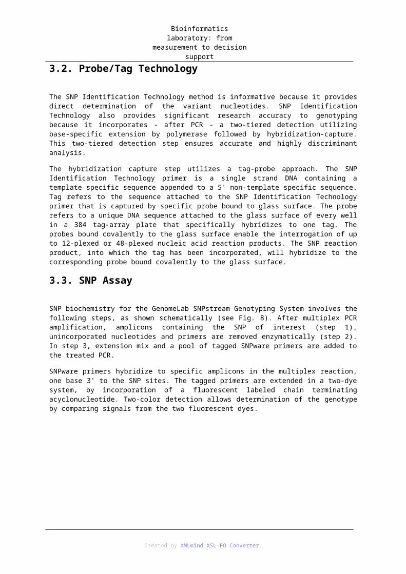
SNP biochemistry for the GenomeLab SNPstream Genotyping System involves the following steps, as shown schematically (see Fig. 8). After multiplex PCR amplification, amplicons containing the SNP of interest (step 1), unincorporated nucleotides and primers are removed enzymatically (step 2). In step 3, extension mix and a pool of tagged SNPware primers are added to the treated PCR.
SNPware primers hybridize to specific amplicons in the multiplex reaction, one base 3' to the SNP sites. The tagged primers are extended in a two-dye system, by incorporation of a fluorescent labeled chain terminating acyclonucleotide. Two-color detection allows determination of the genotype by comparing signals from the two fluorescent dyes.
The extended SNPware primers are then specifically hybridized to unique probes arrayed in each well. The arrayed probes capture the extended products (step 4) and allow for the detection of each SNP allele signal (step 5). Stringent washes remove free dye-terminators and DNA not hybridized to specific probes.
3.4. Control spots
Two self-extending control oligonucleotides are included in each extension master mix and are extended with either the blue or green dye-labeled terminator during the primer extension thermal cycling.
The array of capture oligonucleotides attached to the glass surface in each well of a 384-well plate includes three positive controls and one negative control (see Fig. 9). The XY control spot is a heterozygous control
Created by XMLmind XSL-FO Converter.

Bioinformatics laboratory: from measurement to decision support
which has a mixture of two capture probes that allow hybridization of both blue and green control oligonucleotides. The XX control spot has a capture probe that allows hybridization of the blue control oligonucleotide. The YY control spot has a capture probe that allows hybridization of the green control oligonucleotide.
The primers used in this system to mark the SNPS, are marked with two fluorescent dyes, notably Tamra and FAM, which despite having close emission spectra, are well separated in the systems scanning procedures. Channel crosstalk of less than 3% was observed on the X and Y control points.
After scanning the plates with a narrow band light source, the blue and green images corresponding to the two dyes are recorded for each well. Each sample well is illuminated with a 488-nm and a 532-nm laser beam.
3.5. Digital image processing methods used in genotyping studies
The task of image analysis is to convert the enormous number of pixels in the well images into hybridization values for each sample. Typically genotyping image analysis programs give a few summary statistics of pixel intensities for each spot and for the surrounding background.
Generally there are several stages in image analysis.
3.5.1. Filtering
Filtering is the replacement of each pixel with a value derived from the pixel and other pixels surrounding it. Two types of filters are useful for digital image analysis: median filters and top-hat filters. Both of these filters deal well with high-frequency noise, and their use greatly improves the accuracy of grid alignment.
3.5.2. Grid alignment
Created by XMLmind XSL-FO Converter.

Bioinformatics laboratory: from measurement to decision support
Grid alignment is the process of finding the location of each well in the well image. Generally a fixed grid is positioned over the area and semi-manual adjustments are made to finalize the grid. Each well contains four control spots (X, Y, XY, Negative control) which can be used successfully in securing perfect alignment of the grids to the spots on the images.
3.5.3. Segmentation
After we have found the grid position on each well image, we must also find the location of each spot inside the well image. We need to decide which pixels in the image are part of the spot, and which are part of the background.
3.5.4. Noise patterns
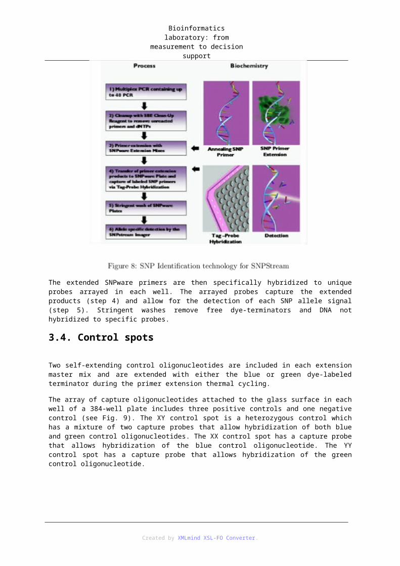
Calculating the intensity is not merely enough to obtain reliable genotyping data from the scanned images, since many artifacts and errors can distort the scanned image, such as those shown (see Fig. 12).
Most of these artifacts can greatly reduce the quality of our measurements, but luckily they can also be
Created by XMLmind XSL-FO Converter.
Bioinformatics laboratory: from measurement to decision support
accounted for and their effects minimized.
3.5.5. Genotyping
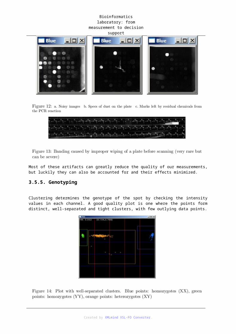
Clustering determines the genotype of the spot by checking the intensity values in each channel. A good quality plot is one where the points form distinct, well-separated and tight clusters, with few outlying data points.
Clustering is the process of selecting all of the spots over the plate corresponding to one SNP, e.g. collecting the same spot in each well, and plotting it according to a score. This two-dimensional plot consists of the following scores: the logarithm (log10(B+G)) of the summed blue and green intensities corresponding to a single spot, versus the ratio of the spots color intensities (B/(B+G)). Based on the position of the data point on the plot in relation to all the other data points within that SNP, we can determine the genotyping of the sample.
Sometimes the clusters are not nearly as well-defined as the one shown above. In this case we can use the Hardy-Weinberg equilibrium principle to calculate how far the clustering places the SNP distribution from the ideal distribution formed by completely random mating in a given population. The HW equilibrium principle provides essential feedback on the feasibility of our measurements; Hardy-Weinberg principle states that both allele and genotype frequencies in a population remain constant. How far a population deviates from HWE can be measured using the "goodness of fit" or chi-squared test ( ). The Hardy-Weinberg equilibrium measurement by chi-squared test is essential for manual clustering.
3.5.6. Artifact suppression
Occasionally, as described above, specs of dust, residual chemicals or wipe marks may be seen on some images. These present a major hazard to the result of the image processing and to the accurate determination of genetic information, therefore they should be eliminated.
The results of artifact suppression on a plot are shown (see Fig. 15).
Created by XMLmind XSL-FO Converter.
Bioinformatics laboratory: from measurement to decision support
3.6. Questions
1. Name three sources of noise in genotyping!
2. How many SNPs can be measured on a chip?
3. What color fluorescent dyes are used?
4. What is the Hardy-Weinberg equilibrium principle?
5. Under what conditions is the Hardy-Weinberg equilibrium principle true?
6. What can be used to copy a strand of DNA?
7. If a human SNP has two alleles, what combinations can occur?
4. 4 Study design: from the basics to knowledge-rich extensions
4.1. Introduction
Biomedical study design is a complex task with the goal of ensuring the optimality of the experiments: gaining the largest possible amount of knowledge with at the lowest possible cost (referring to both theoretical and practical aspects: statistical anomalies, time, money etc.). The knowledge accumulated in the post-genomic era offers unique opportunities in study design: the numerous results obtained in the past can give directions in assembling the experiments in the future. However, the amount of available background knowledge has become simply too enormous for any human to comprehend, far exceeding the capabilities of even the finest scientists. To deal with the situation, study design has turned to computer sciences (particularly data fusion and artificial intelligence) and statistics.
Gene prioritization is a relatively young, but very popular class of methods in the intersection of experimental biology, study design and statistics. It aims to determine an ordering of the genes on the basis of the query - it is
Created by XMLmind XSL-FO Converter.

Bioinformatics laboratory: from measurement to decision support
not particularly surprising that certain systems bear a resemblance to internet search engines. After the first experiments in 2002, a plethora of new gene prioritization software packages were developed, from which - due to their performance - the network- and kernel-based approaches have begun to emerge. Prioritization tools can offer significant help in experimental design, as they can narrow down the set of investigated genes utilizing the otherwise incomprehensible amount of background knowledge.
In this practice, we will become familiar with the kernel-based approaches for gene prioritization. The first of this class of tools, called Endeavour, was published in 2007. The greatest advantage of this system is the convenient and efficient combination of heterogeneous data sources. Similarly to Endeavour, our tool is based on support vector machines (SVM), which are among the most widespread machine learning algorithms.
4.2. SVM-based gene prioritization
The workflow of the SVM-based gene prioritization is depicted in Figure 16. Before going into the details of the inner workings of the algorithms, we review the main steps of the workflow:
1. Choosing candidate genes. Prioritizing the whole genome is certainly possible; however, it can be very impractical. There are a number of reasons for this:
• Human: labor demand (think about it: a list with a couple of hundreds of entities is already very hard to analyze by hand).
• Computational: computational and storage complexity.
• Statistical: prioritizing the whole genome is much more complex task, which is only partially solved at the moment, as several statistical anomalies can occur in these scenarios (see later).
• Biological: "inherently" meaningless entities.
2. Choosing information sources, computing kernels. There are countless information sources available in the form of databases, e.g. sequence, pathway, gene expression etc. databases.
3. A common feature of kernel-based methods is that they consider the data solely in terms of pairwise similarities. The positive semidefinite matrix containing these similarities is called kernel, which is relatively easy to compute for most information sources. We have to specify an appropriate similarity measure: we can choose from "successful" metrics as well as design our own similarity function. Note that the required mathematical machinery for the latter is far beyond the scope of this class, therefore we will not consider this option during this practice.
On the basis of each information source, one or more similarity matrices can be computed using the similarity functions, for which
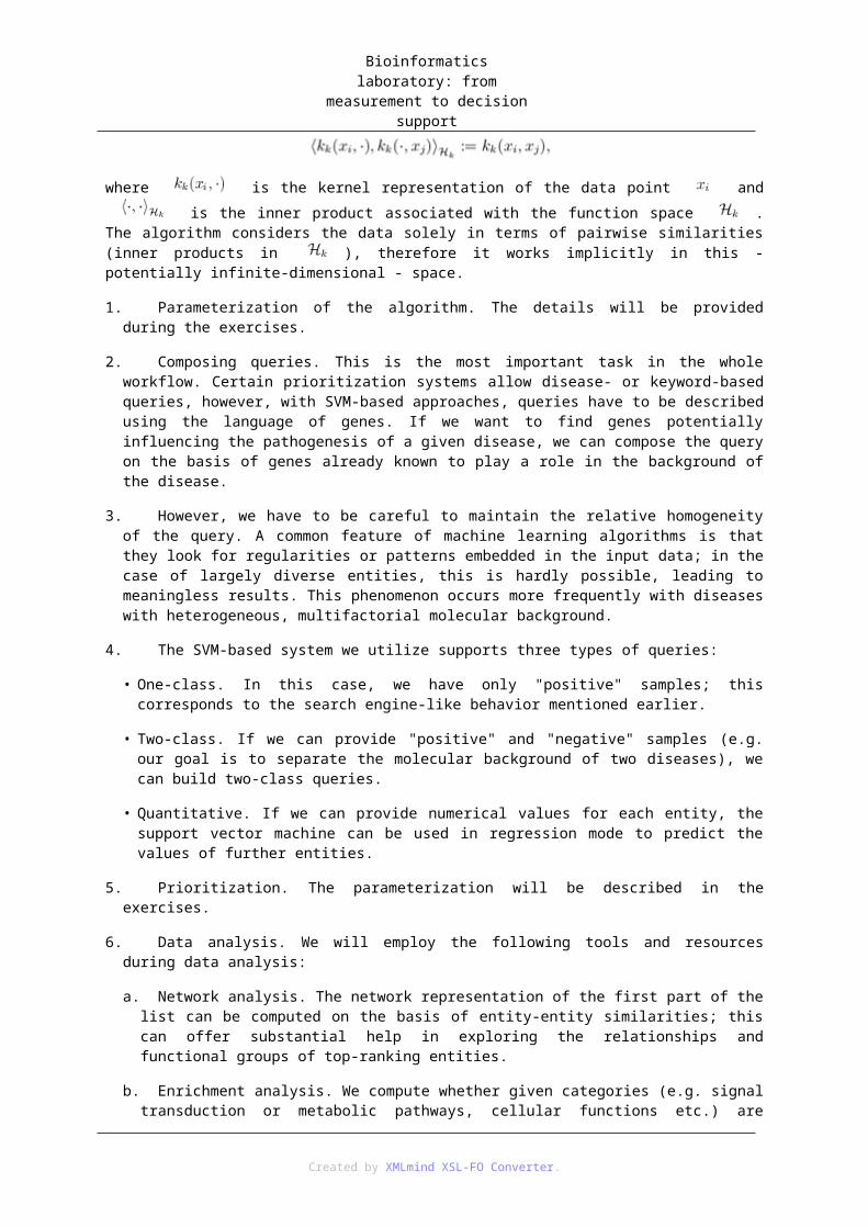
Every positive semidefinite similarity matrix (kernel) defines a Hilbert space, for which
where is the kernel representation of the data point and is the inner product associated with the function space . The algorithm considers the data solely in terms of pairwise similarities (inner products in ), therefore it works implicitly in this - potentially infinite-dimensional - space.
1. Parameterization of the algorithm. The details will be provided during the exercises.
2. Composing queries. This is the most important task in the whole workflow. Certain prioritization systems allow disease- or keyword-based queries, however, with SVM-based approaches, queries have to be described using the language of genes. If we want to find genes potentially influencing the pathogenesis of a
Created by XMLmind XSL-FO Converter.

Bioinformatics laboratory: from measurement to decision support
given disease, we can compose the query on the basis of genes already known to play a role in the background of the disease.
3. However, we have to be careful to maintain the relative homogeneity of the query. A common feature of machine learning algorithms is that they look for regularities or patterns embedded in the input data; in the case of largely diverse entities, this is hardly possible, leading to meaningless results. This phenomenon occurs more frequently with diseases with heterogeneous, multifactorial molecular background.
4. The SVM-based system we utilize supports three types of queries:
• One-class. In this case, we have only "positive" samples; this corresponds to the search engine-like behavior mentioned earlier.
• Two-class. If we can provide "positive" and "negative" samples (e.g. our goal is to separate the molecular background of two diseases), we can build two-class queries.
• Quantitative. If we can provide numerical values for each entity, the support vector machine can be used in regression mode to predict the values of further entities.
5. Prioritization. The parameterization will be described in the exercises.
6. Data analysis. We will employ the following tools and resources during data analysis:
a. Network analysis. The network representation of the first part of the list can be computed on the basis of entity-entity similarities; this can offer substantial help in exploring the relationships and functional groups of top-ranking entities.
b. Enrichment analysis. We compute whether given categories (e.g. signal transduction or metabolic pathways, cellular functions etc.) are significantly over-represented among top-ranking entities.
c. Statistical analysis. Statistical features computed during prioritization can help detecting the inhomogeneity of the query.
d. Scientific literature. Scientific literature (e.g. the Pubmed engine) and expert knowledge aids the interpretation of the results.
Created by XMLmind XSL-FO Converter.
Bioinformatics laboratory: from measurement to decision support
Created by XMLmind XSL-FO Converter.

Bioinformatics laboratory: from measurement to decision support
The one-class algorithm solves the following problem:
Created by XMLmind XSL-FO Converter.

Bioinformatics laboratory: from measurement to decision support
where parameterizes the hyperplane, denotes the kernel weights, denotes the margin, controls the model complexity, is the number of samples, is the vector of the slack
variables, and corresponds to the weight regularization. The algorithm computes the hyperplane farthest away from the origin and closest to the query (denoted with blue color). This also drives the weighting of the data sources; further samples can be prioritized using the distance to the hyperplane:
Figure 17 provides geometrical intuition for understanding the one-class algorithm. Members of the query can be projected to a higher-dimensional space through the kernel. The one-class SVM computes a (hyper)plane which lies as close to the query as possible in this space. Other entities can be prioritized using the distance to the hyperplane.
4.3. Questions
Please answer these questions in 1-2 sentences.
1. Besides those mentioned earlier, what kind of information sources can you imagine in the context of gene prioritization? (3 examples)
2. How would you define the concept of similarity in pathway, sequence, gene expression and the previous three data sources?
3. Why does the problem of heterogeneous queries appear more frequently in multifactorial diseases?
4.4. Exercises
During these exercises, we will select a disease and collect known associated and candidate genes.
1. Select an arbitrary, fairly well-known disease. Consider e.g. various aspects such as known genetic background, prevalence, appearance in media etc.
2. Investigate which genes can, in theory, play a role in the development of the disease. Use the Genetic Association Database (http://geneticassociationdb.nih.gov/) which collects the results of several candidate gene and genome-wide association studies (CGAS and GWAS, respectively). Use the Search link to list genes associated with the selected disease and collect 10-12 hits. In the Problems section, these will play the role of candidate genes; the goal of the study design is to determine the most "promising" ones.
3. Compile a query set, which consists of genes with a presumably significant impact on the development of the disease. Use the DisGeNET database (http://ibi.imim.es/web/DisGeNET/v01/home), which integrates several databases containing gene-disease associations (e.g. manually curated and predicted, even text-mining based ones). Run a query with the selected disease and select 4-5 genes from the top-scoring hits. These will be utilized as a query set (input) to the gene prioritization process.
4. Finally, compile a control set consisting of 3-4 genes which are not known to be associated with the selected disease. Add these genes to the candidate list.
4.5. Problems
Created by XMLmind XSL-FO Converter.

Bioinformatics laboratory: from measurement to decision support
4.5.1. 1. Selecting data sources and similarity measures
The first step in the workflow is adding gene-gene similarity matrices (kernels). The following kernels are available:
• Gene expression-based similarity matrices
• Similarity matrices based on text-mining similarity
• Similarity matrices based sequence similarity
• Pathway-based matrices
• Matrices based on semantic similarities
Start the application, and then use the Browse button to select a kernel. In the Type field, choose the Precomputed option. Since data sources tend to be incomplete, a kernel average value also has to be specified which will be used in place of the missing values; for the sake of simplicity, we set the kernel average to . The kernel can be added to the collection using the Add button. Add at least three kernels.
4.5.2. 2. Prioritizing
Genes in the data sources can be loaded with the Load button. We will use the tool to perform one-class prioritizations. Add the selected genes to the positive group with the Add (+) button or by pressing Enter. You can also search in the list of genes by typing in the first few characters of the gene. You can start the prioritization with the Go button. The pop-up window informs you about various runtime parameters and weights of the information sources. Which information source has achieved the largest weight?
4.5.3. 3. Interpreting the results
Examine the results of the prioritization. The first places are usually occupied by the elements of the query; if it is not so, or if the query has decomposed into multiple blocks, you can suspect an overly heterogeneous query. Inspect the first 10-15 hits. Do you see any "familiar" genes, besides the query? You can also search in the prioritized list by typing the first few characters of a gene.
Determine the positions of each element in the candidate list. Where is the "best" candidate? Where are the other candidates and the elements of the control set? Summarize your findings in 4-5 sentences.
You can display prioritization statistics with the Show plots button. Consider the compactness plot. The x axis represents the first 100 genes. The average similarity of the first x genes is represented on the y axis. This value obviously equals one for the first sample, and it should exhibit a shape resembling the reciprocal function. In the case of overly heterogeneous queries, the curve looks more like a "square root" sign.
You can display the similarity network of the first 50 genes with the Show graph button. The entities are connected on the basis of their combined similarities to each other (considering the weights of the information sources). Specify an appropriate cutoff level and lay out the graph with the Graph layout button. Entities in the first part of the prioritized list are colored pink, the others are blue. Do you see any regularity in the graph?
Choose two arbitrary genes from the graph and investigate their neighbors. Compare this list with that of the DisGeNET database, which you can reveal by searching for the gene name and clicking on "All genes associated with this gene".
Perform the analysis steps above and summarize your findings. You can experiment with different settings, e.g. omitting certain information sources or specifying different parameterizations.
4.5.4. 4. Enrichment analysis
Created by XMLmind XSL-FO Converter.
Bioinformatics laboratory: from measurement to decision support
In this final task, we will search for "enriched" (i.e. most over-represented) pathways and diseases in the prioritized list. Push the Enrichment analysis button, and then browse the disease-based annotation file.
You can adjust the following parameters:
• E-value cutoff: only the categories with an e-value (Bonferroni-corrected p-value) under this cutoff will appear. If there are no results, you can raise this level or disable the cutoff completely to reveal the whole list.
• Hit number cutoff: by default, only the diseases with at least two genes in the list will take part in the analysis.
You can start the analysis with the Analyze button. The first column of the results contains the e-values and the second one contains the category names. Lower ( ) e-values mean that the genes of that particular disease are significantly over-represented among the top-ranking entities of the prioritized list. Do you see the original disease in the list? What other diseases are present? What kind of relations can be hypothesized between diseases with a low e-score (e.g. similar genetic background, comorbidity etc.)?
Perform this analysis using the pathway-based annotation file as well. Which pathways are over-represented? Analyze some of the top-ranking pathways on the list by utilizing the biomedical literature (i.e. the PubMed search engine). Are there any publications proposing a connection between the disease and the pathways?
5. 5 Bioinformatical workflow systems
The program BayesCube performs BMLA analyses through a multi-step workflow hidden from the user. This workflow consists of multiple phases, the overview of which might give a better understanding of BMLA analyses.
In the following, we examine these phases using an example application to manually reproduce each step.
5.1. 5.1 Constructing data and model
BMLA analyses are always based on a set of observation data and the corresponding Bayesian network model, while the primary goal is the examination of the structural relations among nodes of the network.
5.1.1. Tasks.
Construct a simplified model (consisting about 5-6 nodes) for a chosen subject domain using the BayeCube software; specify the relations (edges) within the model and the numerical parameters of the local dependence models.
Generate a sample dataset from the model, then partition it to multiple parts along the values of a selected variable, using a spreadsheet-editing software (e.g. OpenOffice Calc).
5.2. 5.2 BMLA analysis configuration files
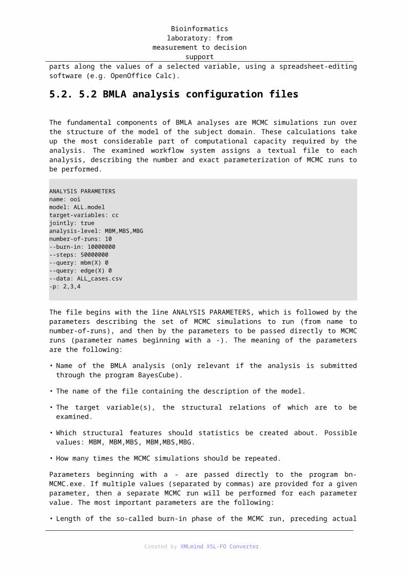
The fundamental components of BMLA analyses are MCMC simulations run over the structure of the model of the subject domain. These calculations take up the most considerable part of computational capacity required by the analysis. The examined workflow system assigns a textual file to each analysis, describing the number and exact parameterization of MCMC runs to be performed.
ANALYSIS PARAMETERSname: ooimodel: ALL.modeltarget-variables: ccjointly: trueanalysis-level: MBM,MBS,MBGnumber-of-runs: 10
Created by XMLmind XSL-FO Converter.

Bioinformatics laboratory: from measurement to decision support
--burn-in: 10000000--steps: 50000000--query: mbm(X) 0--query: edge(X) 0--data: ALL_cases.csv-p: 2,3,4
The file begins with the line ANALYSIS PARAMETERS, which is followed by the parameters describing the set of MCMC simulations to run (from name to number-of-runs), and then by the parameters to be passed directly to MCMC runs (parameter names beginning with a -). The meaning of the parameters are the following:
• Name of the BMLA analysis (only relevant if the analysis is submitted through the program BayesCube).
• The name of the file containing the description of the model.
• The target variable(s), the structural relations of which are to be examined.
• Which structural features should statistics be created about. Possible values: MBM, MBM,MBS, MBM,MBS,MBG.
• How many times the MCMC simulations should be repeated.
Parameters beginning with a - are passed directly to the program bn-MCMC.exe. If multiple values (separated by commas) are provided for a given parameter, then a separate MCMC run will be performed for each parameter value. The most important parameters are the following:
• Length of the so-called burn-in phase of the MCMC run, preceding actual sampling.
• Length of the sampling phase of the MCMC run.
• Name of the .csv file containing the observation data used for the calculation of the score of visited model structures.
• Maximal allowed number of parents for nodes.
• The method by which structure scores are calculated. Possible values: CH, BDeu.
5.3. 5.3 Running under the system HTCondor
The whole process of a BMLA analysis is carried out by the execution of jobs submitted to the HTCondor job management system, according to the following main steps:
1. The submit files describing individual HTCondor jobs are generated in accordance with the previously described configuration file. This step is carried out by the class soapbmla.cmd.GenerateCondorJobs found in the package soapBMLAtools.jar.
2. The program bn-MCMC.exe performs the MCMC simulations; the parameterizations of which are placed in the HTCondor submit files (*.sub) found in the subdirectories calc*.
3. Results of individual MCMC runs are aggregated into one common file by the program mergeResults.exe; the description of the corresponding HTCondor job can be found in the submit file aggregate.sub.
4. Coordination of the above jobs are done by the dagman tool provided by the HTCondor system; the enumeration and precedence order of the jobs is contained by the file dagman.dag, the corresponding submit file is dagman.dag.condor.sub.
5.3.1. Tasks.
Reedit the above configuration file according to the following:
Created by XMLmind XSL-FO Converter.

Bioinformatics laboratory: from measurement to decision support
1. Refer to your own model and data files in the appropriate places, so that model learning will be performed on each data partition separately, and (using one concatenated file of the partitions) on the whole data as well.
2. Specify values for the maximal parent count (parameter -p) and parameter prior (parameter -param-prior, possible values: CH and BDeu) MCMC parameters.
Generate the HTCondor submit files from the configuration file using the following command:
java soapbmla.cmd.GenerateCondorJobs --bayeseye-conf <conf_file> --run false --bin-dir <dir>
Substitute <conf_file> with the name of your on configuration file, and <dir> with the path to the directory containing the program bn-MCMC.exe.
Examine the directories and files generated by the command, then submit the analysis to the HTCondor system using the command:
condor_submit dagman.dag.condor.sub
Later, the command condor_q can be used to list the jobs present in the HTCondor system, and query their state.
5.4. 5.4 Aggregation of raw results
After the completion of HTCondor jobs, the results of individual calculations will be located in the directories *calc*. The aggregation (merging the results of separate runs, calculating basic statistics of them) of these is performed by the program mergeResults.exe. During the aggregation process, the program collects the results (from result files and logs belonging to them) of MCMC runs with parameterizations regarded equivalent, merges them and calculates basic statistics like average and standard deviation. By default, only the results of perfectly identical runs are merged, however, through the arguments of mergeResults.exe we can define parameters to be "aggregated out" (i.e. to perform aggregation over all the runs the parameterizations of which only differ in the values of specified parameters).
According to the help text provided by the program, the main arguments of mergeResults.exe are the following. (+ signs mark those arguments for which multiple values van provided in a space-separated list.)
$ mergeResults.exeUsage : mergeResults.exe <OPTIONS> IGNORE [parameter]+ : the parameter will not be taken into account in differentiating parameter configurations AGGREGATE [parameter]+ : the parameter will be aggregated out GROUP [parameter]+ : different value configurations will be put to different output files
IN [features.csv]+ : input files OUT <output prefix> : prefix of output file names IGNORE-CONSTANTS : do not display constant parameter values AGGREGATES-ONLY : do not print feature probabilities to output PROBS-ONLY : do not print aggregate function values to output ORDER-BY [parameter]+ : order columns in output by given parameter AGGREGATE-FUNCTIONS [name]+ : list of aggregate functions to calculate over results
Created by XMLmind XSL-FO Converter.

Bioinformatics laboratory: from measurement to decision support
with the same parameterization
• The given parameter will not be taken into account, i.e. it will not appear in the output, and it will be "aggregated out".
• The parameter will be "aggregated out".
• A separate output file will be created for each value taken by the specified parameter.
• List of input files.
• Prefix of the output file(s), the program might append further pieces of information to this, e.g. if the argument GROUP was specified.
• The parameters which only take a single value throughout all the runs will not be displayed in the output. (This improves readability.)
• Only aggregate values (like average, standard deviation, etc.) will be written to the output, "raw" probabilities not.
• Opposite of the previous: only "raw" probabilities will be present in the output.
• Columns of the output will be ordered according to the values of these parameters.
• List of aggregate functions to be included in the output. Possible values are: AVG - average, STDEV - standard deviation, STDEV_DIV_AVG ratio of standard deviation to the average, COUNT - number of the input files the given feature value appeared in, MIN - minimum, MAX - maximum.
Hence if we want to get the average and standard deviation of MBS values with the observation data aggregated out in separate output files according to different parameter priors, we can issue the following command:
mergeResults.exe IN *calc*/*MBS*.csv OUT output AGGREGATES-ONLYAGGREGATE-FUNCTIONS AVG STDEV GROUP --data
5.4.1. Tasks.
According to the above, create the aggregated result files separately for each feature type.
Examine how aggregation over different parameters affects the result files.
Open the created result files using the BayesEye software, and examine the effects of aggregation there as well.
5.5. 5.5 Questions
1. What model class is applied in BMLA analyses for the representation of the subject domain?
2. What calculations form the foundations of BMLA analyses?
3. Name the job management system applied for BMLA analyses!
4. What commandline tool can be applied to query the list and state of currently running calculations?
5. Name at least three of the parameters of the program mergeResults.exe!
6. What is the meaning of "aggregating out" a parameter?
6. 6 Standard analysis of genetic association studies
Created by XMLmind XSL-FO Converter.

Bioinformatics laboratory: from measurement to decision support
lab exercise
6.1. 6.1 Introduction
In this lab exercise we perform basic statistical analysis with easy-to-use statistical tools that enable the analysis of the results of genetic association studies. For the exercises we use a previously filtered and preprocessed artificial data set (BIOINFO_LAB_Data.csv) which contains 28 SNPs and a case-control state descriptor as a binary target(variable). The imputation of missing values was already performed.
First we investigate whether Hardy-Weinberg equilibrium (HWE) holds for each of the SNPs, then we perform basic allele and genotype level association tests. The third part consists of the investigation of haplotype associations. Finally, we perform permutation tests in order to validate association test results.
6.2. 6.2 Hardy-Weinberg equilibrium analysis
We perform HWE analysis with a freely available HWE calculator tool [3], which is downloadable from http://ihg.gsf.de/cgi-bin/hw/hwa1.pl. As input the genotype counts of each SNP in case and control samples are required (as shown in Figure 18). The file named BIOINFO_LAB_Counts.csv contains all the necessary counts which can be uploaded separately for a number of SNPs or as a whole file.
The output is generated in a table form containing HWE, scores and p-values of allele and genotype level association tests, and also odds ratios. Figure 19 shows a section of the result table. The leftmost column provides details on the test of HWE for controls. Due to adequate sample size the p-value of Pearson's chi-squared test should be examined. If the p-value is lower than the significance threshold of , then control samples are not in HWE. Since that suggests a measurement or sampling error, the SNP failing HWE for controls has to be excluded from further analysis. In case of the sample data set only SNP12 fails HWE (p=0.000038) out of 28 SNPs.
Created by XMLmind XSL-FO Converter.
Bioinformatics laboratory: from measurement to decision support
6.3. 6.3 Standard association tests
Apart from HWE, several association tests are performed and displayed in the result table. For each SNP there are two sets of tests which differ only in the chosen risk allele. The upper section (Risk allele 2) contains tests that treat allele as the rare or risk allele, whereas in the lower section (Risk allele 1) tests treat as risk allele. In case of the test for allele frequency difference (between cases and controls) sample sizes related to alleles should be used for the score computation. Let denote common homozygote samples,
denote heterozygote samples, and denote rare homozygote samples, then the sample size
related to allele is given as and consequently .
Based on such frequencies a contingency table can be created, e.g. in case of SNP25 () the observed values are
(see Table 1) with corresponding expected values , (computed as row total * column total / full total). Using the formula detailed in the
related book chapter the chi-squared statistic can be computed: , which entails a non-significant p-value of , which means that the difference between the allele frequency in cases and controls is not significant for SNP25.
For heterozygous and homozygous association tests, apart from the common homozygote sample size , the heterozygote and the rare homozygote sample sizes are required respectively. In case of the allele positivity test (i.e. when the risk allele is present in some form), the homozygote genotype consisting of non-risk alleles is compared to heterozygotes and homozygotes carrying the risk allele (e.g.
). In case of SNP17 for example (see Table 2) the chi-squared test for allele positivity () indicates a significant difference ( ) between cases and controls with
respect to the genotype distribution of SNP17.
Furthermore, the rightmost column of Table 19 contains the results of the Cochran-Armitage test of trend ( score and p-value).
Created by XMLmind XSL-FO Converter.

Bioinformatics laboratory: from measurement to decision support
In addition, beside each association test the odds ratio of corresponding genotypes and its confidence interval is computed.
All in all, based on the results SNP17 seems to be in a dependency relationship with the target, as almost all of the tests indicate a significant difference between cases and controls with respect to its distribution. SNPs 7-9 also appear significant in several tests, although these p-values are less significant compared to the ones of SNP17. However, it is important to note that no correction for multiple hypothesis testing was applied so far, although we performed 16 tests for each of the 28 SNPs which amount to a total of 448 tests. Given the significance threshold of this means that in 5 % of the test results, namely in case of 22 tests a significant result arises by pure chance. Therefore it is imperative to validate the results either by applying other methods and performing a comparison, or by applying a proper correction method or permutation tests.
6.4. 6.4 Haplotype association analysis
For the analysis of haplotypes we use Haploview (Barrett et al., Broad Institute) a visualization and analysis tool [1], which is freely available at http://sourceforge.net/projects/haploview/.
In order to begin the analysis two data files are required by the software: a genotype data file containing the case-control designation and additional information on the samples, and also a SNP information file detailing position, allele type and other supplementary information. The data file can be constructed in a number of different formats. For the sake of simplicity we use the linkage format. Let us load the data set in linkage format (BIOINFO_LAB_Haploview_Sample.ped), and the corresponding SNP information file (BIOINFO_LAB_Haploview_Sample.info), as shown in Figure 20.
Created by XMLmind XSL-FO Converter.
Bioinformatics laboratory: from measurement to decision support
Since we intend to analyze the results of a case-control GAS, we select the appropriate switch (Case/Control data), and we also enable association tests by selecting the (Do association test) option. The threshold limiting the distance between tested base pairs should be set as high as possible (e.g. 500000) as we wish to see a broad overview.
6.4.1. 6.4.1 Linkage
The first panel (LD) visualizes various linkage measures. Linkage disequilibrium (LD) means that the frequency of the joint presence of two or more alleles differs from which is expected by chance [2]. For example in case of two SNPs ( , ) their alleles ( ) form haplotypes
with corresponding frequencies, which differ from the corresponding product of allele frequencies ( ). In other words, it always holds that
however, the frequency of a haplotype only equals the product of corresponding alleles in a state of equilibrium
e.g. . Let mark the difference between the frequency of a haplotype in a state of equilibrium ( ) and in a state of disequilibrium (h). Since the frequencies of haplotype values form a distribution, the divergence from a state of equilibrium can be expressed by the following equations
where . The normalized form of is called , and it is frequently used
Created by XMLmind XSL-FO Converter.

Bioinformatics laboratory: from measurement to decision support
as one of the main measures of linkage disequilibrium. is computed as
The LD shows values for all possible allele (SNP) pairs (see Figure 21). The coloring corresponds to (logarithm of odds) value, which is a logarithm of the ratio of two likelihoods, namely the
likelihood that the observed data is the result of a true linkage of SNPs, and the likelihood that the data is due to pure chance. Haploview considers a as a marker suggesting true linkage, and it is colored with various shades of red. Whereas white and blue coloring corresponds to values and
respectively.
6.4.2. 6.4.2 Defining haplotype blocks
Linkage plays a role in defining haplotype blocks by indicating SNPs that are in a dependency relationship. In order to aid the creation of haplotype blocks, the names of SNPs were amended with a gene identifier prefix in case when several SNPs were in the same gene or in neighboring genes.
Figure 21 shows that SNPs within the GN1 gene form a solid block, thus we define these SNPs as block 1 (blocks can be selected by mouse cursor). Block 2 should contain SNP7 and SNP8 belonging to gene GN2, as both SNPs were found significant previously and their value is considerably high which indicates a strong linkage. In contrast SNP6, although it is in the same gene, shows no linkage to either of the SNPs 7 or 8, therefore it should not be included into block 2. SNPs within genes GN3A and GN3B show signs of moderate linkage, and in case of SNP9 in GNA3 some of the tests indicated a significant difference in cases and controls with respect to its distribution. Based on these notions the SNPS 9-11 can be worthy of further investigation as block 3. The linkage between SNP16 in GN4A and SNP17 in GN4B is relatively weak; however SNP17 is one of the most significant results so far, therefore it would be appropriate to investigate its joint effect with SNP16 as block 4.
Apparently, several factors can be considered in the process of creating haplotype blocks. In addition, multiple configurations can be analyzed by multiple tests. In our current exercise we continue with the analysis of the before mentioned four blocks. The distribution of values for each haplotype block can be examined in the Haplotypes panel (see Figure 22).
6.4.3. 6.4.3 Association tests
Created by XMLmind XSL-FO Converter.

Bioinformatics laboratory: from measurement to decision support
Due to the previously made settings (Do association test) Haploview automatically performs an association test for each SNP and also for the newly defined haplotype blocks. Results are displayed within the Association panel, where results of SNP tests can be found in the Single marker tab and results of haplotype tests are shown in the Haplotypes tab.
The single marker test shown in Figure 23 is similar to the previously introduced test of allele frequency difference between cases and controls. By selecting the header (p-value) of the rightmost column results will be ordered according to significance.
The haplotype test applied by Haploview is similar to the single marker test, though instead of relying on single allele frequencies, this test measures the difference in the frequency of haplotype values between cases and controls. By selecting the Haplotypes tab we can investigate the results of association tests related to the haplotype blocks we defined previously (see Figure 24).
Regarding the first haplotype block (GN1) the haplotype value (variant) GGAG has the highest statistic which is although significant ( ), the frequency of the variant however is low (
). Therefore it would be prudent to validate this result by permutation testing. In contrast, both variants of block 2 (GN2) is significant( ). In
Created by XMLmind XSL-FO Converter.

Bioinformatics laboratory: from measurement to decision support
case of block 3 (GN3) there is a variant AAA, which although has a p-value ( ) below the applied significance threshold of , but it would not survive a correction (because of multiple hypothesis testing) or permutation testing. The results of block 4 (GN4) are convincing in case of variants AG and AA.
6.4.4. 6.4.4 Permutation tests
From the aspect of validating results, permutation testing is a valuable tool, which aims to indicate whether results are due to true relationships and effects or only to pure chance. The essence of permutation tests is that the association test is repeated multiple times using a dataset with permuted case-control designations. That is the case-control descriptor is permuted within the data set thus creating 'dummy' data sets. If a significant result is found when using a permuted data set, then that indicates that the original result was possibly due to chance. The permutation p-value measures the number of significant results given repetitions of the association test used with permuted data sets. The more repetitions are made the more robust the measure becomes.
Let us set 1000 permutations for both single marker association tests and haplotype block tests (see Figure 25).
Results indicate that only SNP17 and the variants of the related haplotype block 4 remain significant after permutation tests. All other SNPs and haplotypes have non-significant permutation p-values (p>0.09). Based on this evidence we may conclude that by using classic statistical tools only SNP17 and the haplotype block of SNP16-17 are clearly significant with respect to the target variable.
7. References
• [1] JC. Barrett, B. Fry, J. Maller, and MJ. Daly. 2005. Haploview: analysis and visualization of LD and haplotype maps. Bioinformatics, 21(2):263-265.
• [2] RC. Lewontin and K. Kojima. 1960. The evolutionary dynamics of complex polymorphisms. Evolution, 14(4):458-472.
• [3] TM. Strom and TF. Wienker. Tests for deviation from Hardy-Weinberg equilibrium and tests for association (case-control studies). Institute for Human Genetics, TU Munich, http://ihg.gsf.de/cgi-bin/hw/hwa1.pl
8. 7 Analyzing Gene Expression Studies
Created by XMLmind XSL-FO Converter.

Bioinformatics laboratory: from measurement to decision support
8.1. 7.1 Introduction
In this chapter we reanalyze a gene expression dataset from the original article of Tölgyesi et al. [4]. In their paper, the authors aimed to identify new genes, gene groups and pathways involved in the pathogenesis of experimental asthma using an ovalbumin-induced murine model of asthma. They applied microarray gene expression analysis of the lung at different time points in the asthmatic process.
Our goal in this chapter is to provide an introduction of how to analyze gene expression data.
For the analyses we use BioConductor, which is an open source and open development software project for the analysis and comprehension of genomic data [5]. It is based on the R statistical computing environment; it is free; is supported on Linux/Unix, Mac OS X, and Windows; has a large community of developers and is easily extended through the R scripting language. We assume that the R software is properly installed.
8.1.1. 7.1.1 Dataset
Three groups of mice (6 mice/group) were sensitized and challenged with allergen (OVA), one group (control group) was sensitized and challenged with placebo (PBS) and served as a control. On day 28 and 30, 4 hours after the first and third allergen challenge, the lungs were removed from mice in groups 1 and 2 for further analysis. On day 31, 24 hours after the third (last) allergen challenge mice in group 3 and the controls were anaesthetized, and airway hyper-responsiveness (AHR) was assessed. After the AHR measurements, lung tissue collection were performed, the same way as it was carried out in groups 1 and 2. Lung tissue RNA samples from group 1, 2 and 3 were identically labeled with Cy5 dye, while lung tissue RNA samples from group 4 (control group) were pooled and labeled with Cy3 dye, and served as a common reference [4]. The outline of the experiment is shown in Figure 26. Note that the downloadable experimental data contains four mice per group.
8.2. 7.2 Installation of prerequisites
Open up a terminal (Applications->Accessories->Terminal from the toolbar), and start R.
$ R
Now, you see the R prompt. We are going to install the BioConductor package and other packages we are going to use in this chapter. These installation procedures will take some time.
> # download the BioC installation routines> source("http://bioconductor.org/biocLite.R")> # installing BioConductor
Created by XMLmind XSL-FO Converter.

Bioinformatics laboratory: from measurement to decision support
> biocLite()> # installing other packages used in our analyses> biocLite("GEOquery")> biocLite("oligo")> biocLite("arrayQualityMetrics")> biocLite("genefilter")> biocLite("limma")
8.3. 7.3 Getting the data
For getting the experimental data, we are using GEOquery which is an interface to the Gene Expression Omnibus (GEO) at the NCBI, which holds transcriptomics data in a standardized format. The gene expression experimental dataset is stored in the GEO with a reference number GSE11911. The dataset contains not only the actual gene expression measurement values, but also includes information on the design of the experiment.
The authors used platform GPL4134 which is the short code for the Agilent Whole Mouse Genome Microarray platform that measures 4x44K transcripts at parallel.
First of all we need to acquire the experimental data directly from GEO. We can do this by loading the GEOquery library, and downloading the series matrix of the experiment we want to analyze. The result is an ExpressionSet object which is the standard format in BioConductor to hold a gene expression dataset along with all available experimental information. For an introduction to the using of the ExpressionSet class, see for example [6]. To get the data, type in the following to the R prompt:
> library(Biobase)> library(GEOquery)> gse11911 <- getGEO("GSE11911", GSEMatrix=TRUE)> gse11911 <- gse11911$GSE11911_series_matrix.txt.gz> show(gse11911)
To view the first five rows of the expression measurement data, type in:
> head(exprs(gse11911))
To view the phenotypic data associated with the samples, type in:
> pData(gse11911)
We see that a grouping column that properly describes the group the mice came from is missing from the phenotypic data. To make this up, we supplement the data by typing:
> pData(gse11911)$Group <- c("Group1","Group1","Group1","Group1","Group2","Group2","Group2","Group2","Group3","Group3","Group3","Group3")
The first four samples come from Group 1, the second four come from Group 2, and the third four come from Group 3. Note that the control group (Group 4) is the common reference in all arrays.
8.4. 7.4 Quality Control Checks
As we can see from the phenotypic information, the dataset was normalized by Agilent Feature Extraction 7.5 software. However, before we move on, it is imperative that we do some quality control checks to make sure there are no issues with the dataset. The first thing is to check the effects of the normalization, by plotting a histogram and boxplots of probe intensities after normalization. For this, we use the oligo package:
Created by XMLmind XSL-FO Converter.
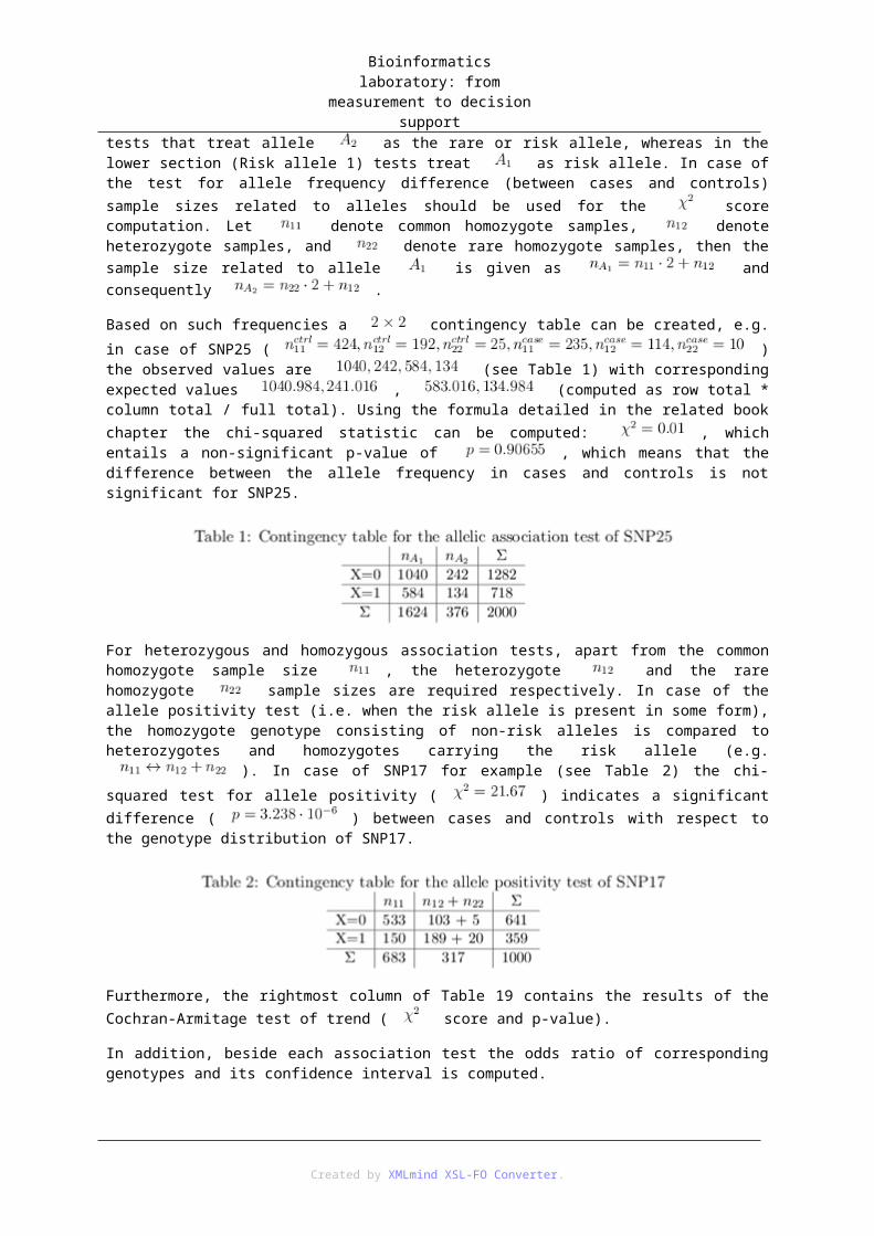
Bioinformatics laboratory: from measurement to decision support
> library(oligo)> hist(gse11911)> boxplot(gse11911, horizontal=T)
Typically, after the normalization the distributions of the arrays should have similar shapes and ranges. Arrays whose distributions are very different from the others should be considered for possible problems. We cannot see any serious problems with the data (see Figure 27).
For advanced quality control checking, we can use for example the arrayQualityMetrics package [7], which produces, through a single function call, a comprehensive HTML report of quality metrics about a microarray dataset. Its main purpose is to aid decision making, by assessing quality of a normalized dataset, in order to decide whether and how to use the dataset (or subsets of arrays in it) for subsequent data analysis [8]. The starting of the quality control process is rather simple, by using the following commands:
> library(arrayQualityMetrics)> arrayQualityMetrics(expressionset=gse11911, outdir="QCreport", force=T, intgroup=c("Group"))
When the function arrayQualityMetrics is finished, a report is produced in the directory QCreport. This directory contains an HTML page index.html that can be opened by a browser. Let's see the result by opening index.html.
8.5. 7.5 Filtering data
Now, after a first glance of the data, we proceed on to analyze it. First, we filter out uninformative data such as control probesets and other internal controls as well as removing transcripts with low variance that would be unlikely to pass statistical tests for differential expression. We are going to use the genefilter package [9] to filter our data.
First, we calculate the interquartile range (IQR) of the signal intensities of all transcripts across the arrays. The IQR equals to the difference between the upper and lower quartiles, . In other words, the IQR is the 1st Quartile subtracted from the 3rd Quartile. Then we estimate the location parameter of the interquartile ranges, using the shorth estimator. The shorth is the shortest interval that covers half of the values in the interquartile ranges. This function calculates the mean of the interquartile range values that lie in the shorth. Type in the following:
> library(genefilter)> IQRs <- esApply(gse11911,1,IQR)> mIQRs <- shorth(IQRs)
To plot the distribution of the interquartile ranges and the location estimate, type in the following (see Figure 28):
Created by XMLmind XSL-FO Converter.
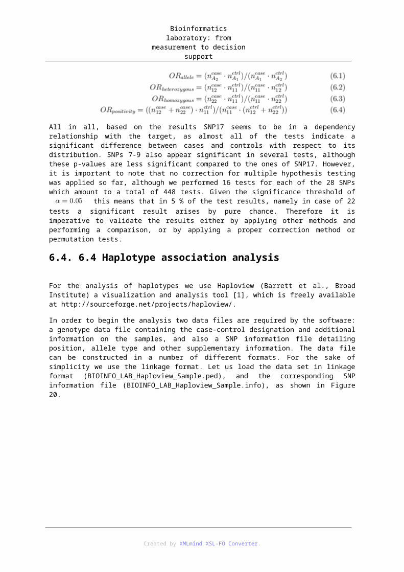
Bioinformatics laboratory: from measurement to decision support
> plot(density(IQRs), xlab="Interquartile range", main="Distribution of IQRs")> abline(v=mIQRs, col="blue", lwd=3, lty=2)
Finally, we filter out those transcripts whose IQR is below the location parameter of all IQRs. In other words, we remove those transcripts whose expression value does not change between the different conditions we analyze (i.e. has low variance). This can be done by typing:
> indices <- genefilter(exprs(gse11911), filterfun(function(x) { IQR(x) > mIQRs }))> gse11911.filtered <- gse11911[indices,]> # see the results of filtering> show(gse11911.filtered)
From among the transcripts the filtering process has kept .
8.6. 7.6 Calculating Differential Expression
Now that we have filtered the dataset, we can proceed with our analysis by identifying those transcripts that are differentially expressed between the experimental groups. For this purpose, we use the limma package [10]. First, we need to construct a so-called model matrix. With this matrix we can easily specify multiway comparisons in complex microarray experimental designs. The design in our case is rather simple; the Cy3 dye-labeled samples are common reference to the other groups labelled with Cy5 dye.
We start by creating a matrix, named targets that indicates which samples are labeled with Cy3 and Cy5 dyes in our arrays:
> targets <- cbind( Cy3=c("Ref","Ref","Ref","Ref","Ref","Ref","Ref","Ref","Ref","Ref","Ref","Ref"), Cy5=pData(gse11911.filtered)$Group )> rownames(targets) <- paste("Array",1:12)> targets
Then, the modelMatrix command creates the design matrix based on the targets matrix we created above:
> design <- modelMatrix(targets, ref="Ref")
Created by XMLmind XSL-FO Converter.

Bioinformatics laboratory: from measurement to decision support
> design
Next, we call the lmFit function to fit a linear model to the data, separately gene per gene. After that we compute moderated t-statistics, moderated F-statistic, and log-odds of differential expression by empirical Bayes shrinkage of the standard errors towards a common value using the eBayes command:
> fit <- lmFit(gse11911.filtered, design)> fit <- eBayes(fit)
Let's see the return value of the above command:
> names(fit) [1] "coefficients" "rank" "assign" "qr" "df.residual" [6] "sigma" "cov.coefficients" "stdev.unscaled" "pivot" "genes"[11] "Amean" "method" "design" "df.prior" "s2.prior"[16] "var.prior" "proportion" "s2.post" "t" "df.total"[21] "p.value" "lods" "F" "F.p.value"
As a first checking of the results, let's see the histogram of the raw -values (see Figure 29).
> hist(fit$p.value, 1000)
The horizontal "floor" of values in this plot corresponds to the features whose target genes are not differentially expressed. The sharp peak at p < 0.001 corresponds to differentially expressed genes. The shape of this histogram can be used to assess an experiment and its analysis: if the peak on the left is missing, this indicates lack of power of the experiment to detect differentially expressed genes. If the remainder of the distribution is not fairly uniform, this can indicate overdispersion and/or a strong interfering effect of another variable, for example, an unintended batch effect [11].
To obtain a summary table of some key statistics for the top ones, type in the following:
> topTable(fit, number=10, adjust="BH")
We can use the decideTests command to classify the series of related t-statistics as significantly upregulated, downregulated or not significant. This command also handles the multiple testing problem by calculating the
Created by XMLmind XSL-FO Converter.

Bioinformatics laboratory: from measurement to decision support
Benjamini-Hochberg corrected -values [12]. Based on the results, we can plot Venn-diagrams to compare the significantly up- and downregulated transcripts between our experimental groups (see Figure 30).
> results <- decideTests(fit, p.value=0.05, lfc=0.5, adjust.method="BH")> vennDiagram(results, include="down", main="Down-regulated")> vennDiagram(results, include="up", main="Up-regulated")
Finally, we can export the table of results of the statistical analysis into a tabulator-delimited file, which we can import, for example, into a spreadsheet program, by using the write.fit command:
> write.fit(fit, file="fit.txt")
9. References
• [4] Gergely Tölgyesi, Viktor Molnár, Ágnes F. Semsei, Petra Kiszel, Ildikó Ungvári, Péter Pócza, Zoltán Wiener, Zsolt I. Komlósi, László Kunos, Gabriella Gálffy, György Losonczy, Ildikó Seres, András Falus, and Csaba Szalai. Gene expression profiling of experimental asthma reveals a possible role of paraoxonase-1 in the disease. International immunology, 21(8):967-975, August 2009. PMID: 19556304.
• [5] Robert C. Gentleman, Vincent J. Carey, Douglas M. Bates and others. Bioconductor: Open software development for computational biology and bioinformatics. Genome Biology, 5:R80, 2004.
• [6] An Introduction to Bioconductor's ExpressionSet Class. http://www.bioconductor.org/packages/devel/bioc/vignettes/Biobase/inst/doc/ExpressionSetIntroduction.pdf
• [7] Audrey Kauffmann, Robert Gentleman, and Wolfgang Huber. arrayQualityMetrics - a bioconductor package for quality assessment of microarray data. Bioinformatics (Oxford, England), 25(3):415-416, February 2009. PMID: 19106121 PMCID: PMC2639074.
• [8] Introduction: microarray quality assessment with arrayQualityMetrics. http://www.bioconductor.org/packages/2.13/bioc/vignettes/arrayQualityMetrics/inst/doc/arrayQualityMetrics.pdf
• [9] R. Gentleman, V. Carey, W. Huber, and F. Hahne. genefilter: methods for filtering genes from microarray experiments. R package version 1.40.0, http://www.bioconductor.org/packages/2.13/bioc/vignettes/genefilter/inst/doc/howtogenefilter.pdf
• [10] Gordon K. Smyth. Linear models and empirical bayes methods for assessing differential expression in microarray experiments. Statistical applications in genetics and molecular biology, 3:Article3, 2004. PMID: 16646809.
Created by XMLmind XSL-FO Converter.

Bioinformatics laboratory: from measurement to decision support
• [11] Florian Hahne. Bioconductor case studies. Springer, New York, N.Y., 2008.
• [12] Yoav Benjamini and Yosef Hochberg. Controlling the False Discovery Rate: A practical and powerful approach to multiple testing. Journal of the Royal Statistical Society. Series B (Methodological), 57(1):289-300. January 1995.
10. 8 Bayesian, systems-based biomarker analysis
Bayesian, systems-based biomarker analysis methods provide a unique possibility to investigate directness, effect strength, multivariate necessity and sufficiency, predictive power and causality of candidate biomarkers. We focus on the exploration of the posterior over the sets of necessary and sufficient predictors. Specifically, we experiment with a multilevel conceptualization of relevance, which allows a data-driven deep visualization of necessarily or sufficiently relevant predictors. We introduce and illustrate the concepts of relevance map, sub-relevance map, sup-relevance map, relevance tree and relevance interaction.
10.1. 8.1 Introduction
The Bayesian network model class, consisting pairs of a Directed Acyclic Graph (DAG) and its parameters, provides a unique possibility for the normative combination of potentially causal prior knowledge and data, which also can contain interventional variables. In the acausal, probabilistic interpretation, the hypotheses are the observational equivalence classes, i.e. the represented independency model (see the Probabilistic Graphical Models chapter of the Probabilistic Decision support course). In the Bayesian statistical framework, an efficiently computable closed form can be derived for the posterior of an observational equivalence class (for assumptions, see corresponding chapters of the Intelligent Data Analysis course):
In case of acausal structure prior and likelihood equivalent parameter prior, it holds that and for any DAG . Thus, if DAGs
are used as representations of observational equivalence classes, then we can simplify the notation and use only (e.g. the cardinality of will not bias the posterior). The posterior can be used to induce the following posterior over the sets of predictors, which is one of the central element of the Bayesian network based multilevel analysis of relevance (BMLA):
where denotes the parents, children and other parents of the children of node . This posterior can be interpreted as a posterior over the Markov boundary sets of target variable , because Bayesian network structures are almost always, i.e. with probability 1, exact representations in the Bayesian statistical framework [15], and for stable distributions forms a unique and minimal Markov blanket of , (i.e. the Markov boundary of ) [16 és 17].
The induced (symmetric) pairwise relation w.r.t. between and is called Markov blanket membership
The MBM features give an overall characterization of strong relevance of the predictors, or even of the complete domain if the MBM posterior is generated for each node. However, they cannot represent the joint relevance of the predictors, because of their pairwise nature. At the other extreme Markov Boundary sets characterize the joint strong relevance of predictors, but the number of the MB sets is exponential, which is intractable computationally and statistically. The concept of k-ary Markov Boundary subsets is based on sized sets of variables [13].
Created by XMLmind XSL-FO Converter.

Bioinformatics laboratory: from measurement to decision support
Definition 1. For a distribution with Markov Boundary set , a set of variables is called sub-relevant if it is a k-ary Markov Boundary subset (k-subMBS), i.e. and . A set of variables is called sup-relevant if it is a k-ary Markov Boundary superset (k-supMBS), i.e.
and .
The k-subMBS and k-supMBS concepts express the presence or the absence of relevant variables. A k-subMBS set contains those variables that are strongly relevant (i.e. a k-subMBS denotes a "necessary" set of variables). The complement of a k-supMBS set contains variables that are not strongly relevant (i.e. a k-supMBS denotes a "sufficient" set of variables). Note that the k-subMBS and k-supMBS concepts form hierarchically related, overlapping hypotheses. Indeed, the scalable polynomial cardinality of the set of k-subMBSs and k-supMBSs is bridging the linear cardinality of the MBM features and the exponential
complexity of the MBS cardinality ( ), where denotes the number of observed variables. Because the cardinality of the MBGs and DAGs are even higher [45], we can think of MBMs, k-subMBSs/k-supMBSs, MBSs, MBGs, and DAGs as more and more complex hypotheses about relevance. In short, they form a hierarchy of levels of abstraction to support a multilevel analysis, in which intermediate levels of k-MBS for varying allow a scalable partial multivariate analysis focusing on
number of variables.
In the Bayesian framework, the posterior probability of the sub-relevance of a subset is:
Analogously, the posterior probability of sup-relevance is computed as follows:
The k-subMBS posteriors allow a relevance based score to characterize statistical interaction:
This systems-based approach formalizes the intuition that relevant input variables with decomposable roles appear independently in the model. If the k-subMBS posterior of set is larger than its approximation based on MBM posteriors, it may indicate that the variables in set have a joint parameterization expressing non-linear joint effects. In contrast, in case of k-subMBS including redundant variables, the posterior is smaller than its approximation based on MBM posteriors, because the joint presence of the redundant variables in the model is suppressed.
10.2. 8.2 Questions/Reminder
1. What is Feature Subset Selection (FSS) problem?
2. What is the definition of strong and weak relevance?
3. What is the definition of Markov Blanket and Markov Boundary? What is their relevance in diagnosis and prediction?
4. What are the graphical representation of a Markov Boundary in Bayesian networks and Markov networks?
10.3. 8.3 Exercises
Assuming an MBS posterior for a given target variable:
Created by XMLmind XSL-FO Converter.
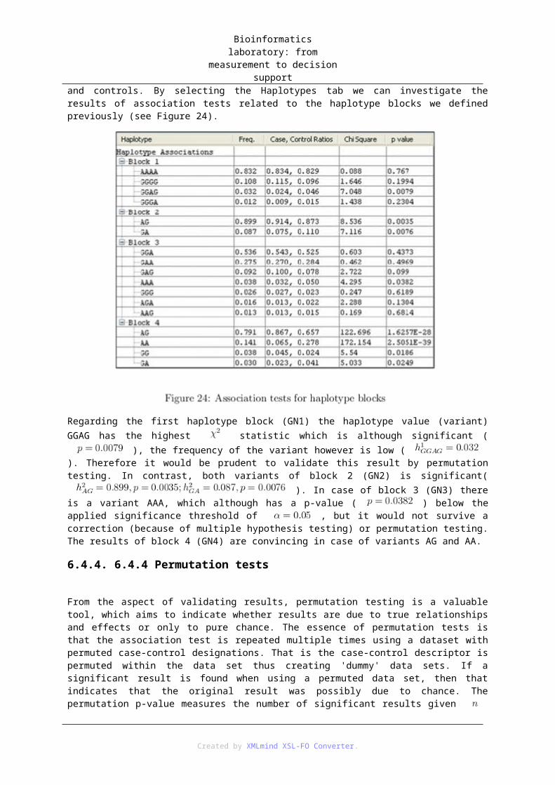
Bioinformatics laboratory: from measurement to decision support
1. Investigate the slope of the ranked MBS posteriors.
2. Investigate the MBM-based approximation of the MBS posterior.
3. Visualize the MBM posteriors using the node-based heat map.
4. Visualize the MBS posterior using the node-based heat map. Explore the conditioning option using Boolean expression over MBSs.
5. Visualize the MBS posterior using the subset lattice, i.e. the relevance map.
6. Compute the maximal k-subMBS and k-supMBS curves, characterize the certainly necessary and certainly not necessary predictors.
7. Construct the relevance tree and interpret fragments of relevance variables.
8. Compute interaction map and interpret relevance-based statistical redundancies and interactions.
10.4. 8.4 Postprocessing and visualization of MBS posteriors
The main concepts for postprocessing and visualization of MBS posteriors are the following (see BayesEye manual for details about the GUI).
10.4.1. 8.4.1 Conditional visualization of MBS posteriors over the model structure
The layout of Bayesian network can be used to visualize the MBSs and the marginal MBM posteriors corresponding to a conditional MBS posterior of the form , where is an arbitrary Boolean expression about the MBS status of the predictors. Fig. 31 illustrate this option and shows the tools for defining such a Boolean expression.
Created by XMLmind XSL-FO Converter.

Bioinformatics laboratory: from measurement to decision support
10.4.2. 8.4.2 The subset lattice for the visualization of MBS and k-MBS posteriors
Both visualization and post-processing can exploit the property that the subsets of predictors form a lattice with operations intersection and union, where the minimum and maximum are the empty and complete sets. We use a transitive reduction map (TRM) of this lattice, where the nodes in the k-th column represent the subsets with size (see Fig. 32). The TRM can be visualized by a DAG where edges denote the "part of" relation, e.g. for a node representing a subset with size has incoming edges from its -sized subsets and outgoing edges to its -sized supersets.
Created by XMLmind XSL-FO Converter.

Bioinformatics laboratory: from measurement to decision support
Figures 33 and 34 show the the visualization of an MBS and k-MBS posteriors over the subset lattice.
Created by XMLmind XSL-FO Converter.

Bioinformatics laboratory: from measurement to decision support
Created by XMLmind XSL-FO Converter.
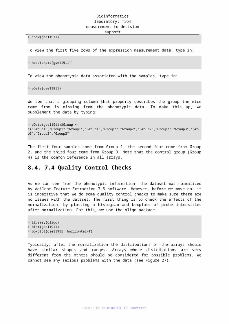
Bioinformatics laboratory: from measurement to decision support
10.4.3. 8.4.3 The relevance tree
The relevance tree shows the subsets in the -Border sets for various thresholds denoting their subset relations with arrows (see Fig. 35). The subset members are indicated incrementally. The size, color, and horizontal position of a set correspond to its sub-Relevance. A -Sub-Relevance Border can be read-off from the tree by an upward search identifying the first nodes with sub-Relevance above the threshold . Note that a -Sub-Relevance Border cannot be read-off exactly for an arbitrary threshold .
Created by XMLmind XSL-FO Converter.

Bioinformatics laboratory: from measurement to decision support
10.4.4. 8.4.4 The relevance interactions
The pairwise, relevance-based statistical interactions can be visualized on relevance interaction chart, see 36. Here the strong relevance of factors (e.g. SNPs) is indicated by bars in the inner circle, the inner segments represent higher level aggregate (e.g. genes), ant the outer segments represent highest level entities (e.g.
Created by XMLmind XSL-FO Converter.

Bioinformatics laboratory: from measurement to decision support
chromosomes). The thicknesses of the edges are proportional with strength of interactions (red) and redundancy (blue).
11. References
• [13] P. Antal, A. Millinghoffer, G. Hullám, Cs. Szalai, and A. Falus. A Bayesian view of challenges in feature selection: Feature aggregation, multiple targets, redundancy and interaction. Journal of Machine Learning Research: Workshop and Conference Proceedings, 4:74-89, 2008.
• [45] G. F. Cooper and E. Herskovits. A Bayesian method for the induction of probabilistic networks from data. Machine Learning, 9:309-347, 1992.
• [15] C. Meek. Causal inference and causal explanation with background knowledge. In Proc. of the 11th Conf. on Uncertainty in Artificial Intelligence (UAI-1995), pages 403-410. Morgan Kaufmann, 1995.
• [16] J. Pearl. Probabilistic Reasoning in Intelligent Systems. Morgan Kaufmann, San Francisco, CA, 1988.
• [17] I. Tsamardinos and C. Aliferis. Towards principled feature selection: Relevancy, filters, and wrappers. In Proc. of the Artificial Intelligence and Statistics, pages 334-342, 2003.
12. 9 Fusion and analysis of heterogeneous biological data
12.1. Introduction
A major hallmark of the post-genomic era is the stunning amount of heterogeneous biological data. The parallel evolution of measurement technologies and computer sciences has made the joint investigation of separate omic
Created by XMLmind XSL-FO Converter.

Bioinformatics laboratory: from measurement to decision support
levels possible, which became the new paradigm for biomedical researches. Therefore, the older field of data fusion began to form strong connections with the much younger bioinformatics and, later, drug discovery.
In the past decade, the numbers of new molecular entities produced by pharmaceutical companies have been diminishing, while the costs of de novo drug development climbed higher and higher. Several strategies were developed to deal with the situation, one of them being the idea of drug repositioning. Drug repositioning means the application of approved drugs in a new indication, which represents a cheaper, faster (repeating preclinical toxicology studies is not necessary), and safer alternative considering the chances of failure. Many systems were developed in the past few years which support in silico drug repositioning; these methods gradually drifted closer and closer to the field of data fusion. During this practice, we will become familiar with such a system.
12.2. Similarity-based prioritization
Data fusion methods can be classified into three groups: early (data-level), intermediate and late (decision-level). Early fusion refers to the direct integration of data (e.g. concatenation); during late fusion one analyzes data from each source separately and combines the results of these analyses. In this practice, we will utilize intermediate fusion, i.e., we employ an intermediate representation of the data to perform the fusion. This representation will consist of similarity matrices of drugs, but before that, we need to examine the concept of similarity.
The "similar property principle" is a well-known concept in the pharmaceutical industry, and (in its original statement) refers to the similar functions of chemically (structurally) similar molecules. This phenomenon was first exploited at the end of the '90s; in silico searching for molecules similar to successful drugs provided promising results. The idea was extended numerous times since then; one such extension considers groups of drugs instead of individual ones, another utilizes more similarity measures simultaneously. The latter is essentially a late data fusion method, where multiple rankings are constructed on the basis of multiple similarity measures, which are then combined using rank fusion methods.
Kernel-based data fusion also utilizes pairwise similarities, however, it outperforms the previous technique in both accuracy and performance. One of its greatest advantages is the adaptive fusion; the weighting of the information sources is driven by the information content of the query (training set), as opposed to previous methods performing global fusion. To understand this, here we provide a simple example.
Consider the following question: which resembles to both a cherry and a small red rubber ball? In the context of shape, we can think of small, round things; in the context of color, we can imagine red objects. In the context of taste these two entities are very far from each other, therefore the question is hard to answer. As a conclusion, we can say that shape and color are "useful" information sources while taste is "useless", however, this can play out very differently when considering different queries. Therefore, mathematically speaking, we assign higher weights to representations of the data in which the elements of the query are "closer" to each other, i.e. they form a set with a small "volume".
On the basis of each information source, one or more similarity matrices can be computed using similarity metrics, for which
Every positive semidefinite similarity matrix (kernel) defines a Hilbert space, for which
where is the kernel representation of the data point and is the inner product associated with the function space . Information sources where the representations of the data form a "small volume" set are assigned higher weights.
The tool used in this practice utilizes the one-class Support Vector Machine (SVM) to automatically weight the information sources and compute a ranking of the drugs (prioritization) on the basis of the query. The details are illustrated in Figure 37.
Created by XMLmind XSL-FO Converter.

Bioinformatics laboratory: from measurement to decision support
Homogeneity of the query set is very important in prioritization. As the weighting of the information sources is essentially governed by the various degrees of heterogeneity, some amount of heterogeneity is desirable, however, researches investigating the performance of the method showed that overly heterogeneous queries exert severe confounding effects. These depend on many factors (e.g. weight regularization, number of information sources etc.), and in some cases, it can result in complete meaningless rankings.
Assuming that , i.e., every entity has a similarity of to itself, then data points lie on the surface of a unit hypersphere in kernel space. The algorithm solves the following problem:
where parameterizes the hyperplane, denotes the kernel weights, denotes the margin, controls the model complexity, is the number of samples, is the vector of the slack
variables, and corresponds to the weight regularization. The algorithm computes the hyperplane which is the farthest away from the origin and slices of the spherical cap containing the entities of the query. The closer these entities are, the larger the margin will become; therefore, the weighting of the information sources can be performed on the basis of the margin. Further entities can be prioritized using the distance from the hyperplane.
One-class SVM and prioritization. The query denoted by is inhomogeneous in the first information source, therefore this source gets a small weight; it would have gained a large weight for the query .
In this practice, we will utilize prioritization to predict potential drug repositionings. This can take place in two contexts. We can start out with an indication (disease) and try to find applicable drugs, or we can start out a drug (e.g. one for which the patent rights have expired or it failed or has been withdrawn) and search for new indications. In the former case, we have to specify a query which characterizes the indication being investigated; this can be achieved easily by selecting drugs which are approved in that particular indication. However, we have to be careful about the homogeneity of the query, especially when considering diseases with heterogeneous molecular background. We can assume that the first entities in the prioritized list can play a role in the treatment of the disease.
If we search for new indications for drugs (or drug combinations), the query consists of these drugs. We can perform an enrichment analysis after the prioritization, which finds out whether drugs from a given indication are significantly over-represented among the top-ranking entities of the prioritized list.
Created by XMLmind XSL-FO Converter.

Bioinformatics laboratory: from measurement to decision support
12.3. Questions
Please answer these questions in 1-2 sentences.
1. Besides the chemical similarity, what kind of information sources can be utilized in drug prioritization? (You will see some examples in the exercises, but many more are readily available.)
2. What information sources can you imagine in the context of gene prioritization?
3. What other intermediate representations can be utilized when performing data fusion? (2 examples)
4. What are the differences between global and adaptive data fusion?
12.4. Exercises
1. You can find information about FDA-approved drugs at the www.drugs.com website. Choose an arbitrary disease and determine how many drugs are approved for its treatment. An off-label drug for a given disease is a compound which is approved in other indications, but not for the treatment of the current disease; however its prescription is generally accepted in the clinical practice. Determine the number of off-label drugs for the selected disease. Remember to write down 4-5 of the approved and off-label drugs, as you will need them later.
2. You can find information about ongoing clinical trials at the www.clinicaltrials.gov website. Search the database by entering your disease in the search field, and then determine the number of ongoing trials and their phase (use the advanced search option).
3. The most important feature of "multifactorial" diseases is that their etiology cannot be linked to a few well-known genes; instead, their etiology depends on a large number of genes, environmental and lifestyle variables. Such diseases include e.g. asthma or type II diabetes mellitus. Search the database at www.godisease.com for your selected disease. How many hits did you get?
4. Www.drugbank.ca contains more information about drugs. Search the database for the drugs you selected at Exercise 1. Look up the "Targets" field. How many targets do the drugs have? How does this number compare to the number of genes in the previous Exercise?
5. At http://sideeffects.embl.de you can find side-effects for many drugs. Select a drug from your previous list and investigate its side-effects. Which are the most frequent?
12.5. Problems
12.5.1. 1. Selecting data sources and similarity measures
The first step in the workflow is adding data sources. Data sources contain the vectorial description of the entities in sparse format. Kernels are computed by the tool on the basis of these descriptions. This requires the selection of a similarity measure for each data source, and their parameterization as well if needed. Since data sources tend to be incomplete, a kernel average value also has to be specified which will be used in place of the missing values.
Start the application, and then use the Browse button to select a data source. In the Type field, select an appropriate similarity measure. The Tanimoto similarity is recommended for chemical information sources and the cosine for others, however, you do not have to stick with these choices (you will also have opportunity to try others later). For the sake of simplicity, we leave the kernel average value as default. The information source can be added to the collection using the Add button.
Created by XMLmind XSL-FO Converter.
Bioinformatics laboratory: from measurement to decision support
Add further information sources:
• Chemical: MACCS fingerprints, 3D pharmacophore-based description, MolconnZ fingerprints
• Side-effect: SIDER (side-effect frequencies), TFDIF (text mining-based side-effect profiles)
• Target profiles: DrugBank
12.5.2. Composing queries, prioritizing
Composing queries is the most important step in the workflow. Select three arbitrary indications (diseases), and then, using your previous exercises or the ATC classification (http://www.genome.jp/kegg-bin/get_htext?br08303.keg), compose a query of 3-5 elements for each disease. Be careful about heterogeneity: for example, the "antidotes" group in the ATC classification is a bad choice, because it is a collective category with its elements having little connection to each other on the biochemical level. You are encouraged to select diseases with well-known molecular backgrounds.
Drugs in the data sources can be loaded with the Load button. The tool supports one- and two-class prioritization and support-vector regression; this time we will use only the one-class method. Add the selected drugs to the positive group with the Add (+) button or by pressing Enter. There are five parameters in the window; we need to concern ourselves with only two of these in the one-class prioritization context:
• controls the weight regularization; high values result in a more uniform distribution of the information sources. It takes values from the interval.
• : in practice, it controls the tolerance to outliers (entities "away" from the remaining part of the query). In the case of high values, there is only little emphasis on the outliers. It takes values from the interval.
You can start the prioritization with the Go button. The pop-up window informs you about various runtime parameters and weights of the information sources. If possible (rarely), you can try to interpret this result: for which indication which information source got the largest weight? Why?
Created by XMLmind XSL-FO Converter.

Bioinformatics laboratory: from measurement to decision support
12.5.3. 3. Interpreting the results
Examine the results of the prioritization. The first places are usually occupied by the elements of the query; if it is not so, or if the query has decomposed into multiple blocks, you can suspect a heterogeneous query. Investigate the first 10-15 hits on the basis of the drug classifications, and use the PubMed search engine (e.g. enter the drug and the disease and see if there are any results; you can also read some of the abstracts). Do the results make sense? Are there any drugs which are not approved in your indication, but their appearance is reasonable based on your findings?
Created by XMLmind XSL-FO Converter.

Bioinformatics laboratory: from measurement to decision support
You can display prioritization statistics with the Show plots button. Consider the compactness plot. The x axis represents the first 100 drugs. The average similarity of the first x samples is represented on the y axis. This value obviously equals one for the first sample, and it should exhibit a shape resembling the reciprocal function. In the case of overly heterogeneous queries, the curve looks more like a "square root sign".
You can display the similarity network of the first 50 drugs with the Show graph button. The entities are connected on the basis of their combined similarities to each other (considering the weights of the information sources). Specify an appropriate cutoff level and lay out the graph with the Graph layout button.
Entities in the first part of the prioritized list are colored pink, the others are blue. Do you see any regularity in the graph? Try to explain the various components using the drug classifications. In the graph below, some drug classes are clearly visible: proton pump inhibitors, 1-receptor antagonists, anticancer drugs, reverse transcriptase inhibitors and other antiviral agents.
Created by XMLmind XSL-FO Converter.

Bioinformatics laboratory: from measurement to decision support
Perform these steps for all of your queries and summarize your findings in 10-15 sentences. You can experiment with other settings, e.g. leaving out certain information sources and using alternative similarity measures or parameters.
12.5.4. 4. Enrichment analysis
In this final task, we will search for new indications for a given drug. Select one (or more) arbitrary drug from the list and add it to the query. Be careful to select one which is present in all information sources. You can check this by performing the prioritization: if a source gets 0 weight, there is no information available about the drug in that source. Push the Enrichment analysis button, and then browse the ATC annotation file.
You can adjust the following parameters:
• E-value cutoff: only the categories with an e-value (corrected p-value) under this cutoff will appear. If there are no results, you can raise this level or disable the cutoff completely to reveal the whole list.
• Hit number cutoff: by default, only the categories with at least two elements on the list will take part in the analysis.
You can start the analysis with the Analyze button. The first column of the results contains the e-values and the second one contains the category names. Lower ( ) e-values mean that the elements of that particular ATC group are significantly over-represented among the top-ranking entities of the prioritized list.
Created by XMLmind XSL-FO Converter.

Bioinformatics laboratory: from measurement to decision support
Do you see the original indication of the drug? What others are present? How can you interpret these findings?
13. 10 Bayesian, causal analysis
Bayesian, systems-based biomarker analysis methods provide a unique possibility to investigate directness, effect strength, multivariate necessity and sufficiency, predictive power and causality of candidate biomarkers. We focus on the exploration of the posteriors over causal features characterizing the whole domain and the sets of necessary and sufficient predictors.
13.1. 10.1 Introduction
In the causal interpretation, the structure of a Bayesian network model (Causal Bayesian network, CBN), can be interpreted as a causal structure, where the nodes represent random variables and edges denote direct influences (see the Causal Bayesian Networks chapter of the Probabilistic Decision support course). This probabilistic approach to causation has many frequently criticized limitations, such as its assumption about the sufficiency of the causal approach (formalized in the Causal Markov Assumption, CMA), its assumption of a stable, underlying distribution (for the necessity of the causally interpreted relations by the edges in the causal structure), it is strict assumption of model minimality, and its inability to formalize contrafactual inference (cf. functional Bayesian networks) [18 és 19]. Despite the limitations, causal Bayesian networks provide a unique possibility for the normative combination of potentially causal prior knowledge and data, which can also contain interventional variables, especially that the omic approach in the postgenomic era somewhat mitigates the problem of CMA. The Bayesian statistical framework, an efficiently computable closed form can be derived for the posterior of a causal structure (for assumptions, see corresponding chapters of the Intelligent Data Analysis course):
where the data can contain interventional variables as well. The posterior can be used to induce distributions over causal model properties, i.e. features, such as edges, compelled edges, Markov Boundary Graph (MBGs), pairwise and complete ordering of the variables. The MBG posterior is one of the central element of the Bayesian network based multilevel analysis of relevance (BMLA):
Created by XMLmind XSL-FO Converter.

Bioinformatics laboratory: from measurement to decision support
Note that the posterior of pairwise relation is defined as follows:
Table 3 shows graphical model based definition of types of associations, relevances and causal relations.
In case of multiple target variable, more refined relations can be defined, such as in Table 4.
The pairwise transitive causal relevance ( ) can be extended a posterior over the complete orderings (permutations) of the variables can be also induced:
13.2. 10.2 Questions/Reminder
1. What is the Causal Markov Assumption?
2. What are a v-structure, essential graph and a compelled edge?
3. What are the ideal intervention, do() semantics and graph surgery?
13.3. 10.3 Exercises
Assuming an edge and an ordering posterior, and an MBG posterior for a given target variable:
1. Visualize the edge posteriors using the model-based layout.
Created by XMLmind XSL-FO Converter.

Bioinformatics laboratory: from measurement to decision support
2. Visualize the MBG posterior using the model-based layout. Explore the conditioning option using Boolean expression over MBGs.
3. Compute the expected order of the variables.
4. Compare the edge posteriors and the ordering posterior.
5. Standardize the multitarget posterior to analogous single target quantities.
13.4. 10.4 Conditional visualization of MBG posteriors over the model structure
The layout of Bayesian network can be used to visualize the MBGs and the marginal edge posteriors corresponding to a conditional MBG posterior of the form , where is an arbitrary Boolean expression about the MBG status of the predictors. Fig. 38 illustrate this option and shows the tools for defining such a Boolean expression (see BayesEye manual for details about the GUI).
13.5. 10.5 Visualization of posteriors over pairwise relation using the model layout
The layout of a Bayesian network can be also used to visualize the pairwise edge and MBM posteriors (see Fig. 39).
14. References
• [18] C. Glymour and G. F. Cooper. Computation, Causation, and Discovery. AAAI Press, 1999.
• [19] J. Pearl. Causality: Models, Reasoning, and Inference. Cambridge University Press, 2000.
15. 11 Knowledge engineering for decision networks
Created by XMLmind XSL-FO Converter.

Bioinformatics laboratory: from measurement to decision support
In which we experiment with various construction methods to build Bayesian networks and decision networks. We explore simple and complex inference methods, and perform a sensitivity of inference analysis related to the value of perfect information. We also investigate the effect of structure on the complexity of inference.
15.1. 11.1 Introduction
The Bayesian network model class has a central position in artificial intelligence:
1. As a probabilistic logic knowledge base, it provides a coherent framework to represent beliefs (see Bayesian interpretation of probabilities).
2. As a decision network, it provides a coherent framework to represent preferences for actions.
3. As a dependency map, it explicitly represents the system of conditional independencies in a given domain.
4. As a causal map, it explicitly represents the system of causal relations in a given domain.
5. As a decomposable probabilistic graphical model, it parsimoniously represents the quantitative stochastic dependencies (the joint distribution) of a domain and it allows efficient observational inference.
6. As an uncertain causal model, it parsimoniously represents the quantitative, stochastic, autonomous mechanisms in a domain and it allows efficient interventional and counterfactual inference.
The goal of the laboratory is to demonstrate and practice this multifaceted nature of Bayesian networks (see corresponding chapters of the course Probabilistic Decision Support).
15.2. 11.2 Questions/Reminder
1. What is the ancestral (topological) ordering of the variables in a Bayesian network?
2. How can we construct an ordering of the variables, which allows an efficient Bayesian network construction?
3. What is a provable correct method to build a Bayesian network compatible with a given ordering of the variables?
4. What is time and space complexity of exact inference in a (poly)tree and in a general Bayesian network?
5. What is the value of perfect information?
6. What is the maximum expected utility principle?
15.3. 11.3 Steps of knowledge engineering
The general steps of the "classical" knowledge engineering of Bayesian networks are synchronous with the general knowledge engineering of logical knowledge bases [42].
1. Identification of purpose, scopes and levels. The major factors underlying the purpose of Bayesian network modeling are the following: probabilistic or causal interpretation, structural or parametric level, decision-support or explanation, domain-wide or classification (i.e., are there any specifically interesting variable(s) or model feature). Next a reasonable scope and level have to be identified including variables and a level of granularity.
2. Collection of informal knowledge. Make a list of all prior knowledge about variables, discretizations, existing dependency models. Classify different types of priors that exist (from exactly specified prior sub-models to high level guesses about qualitative dependencies). Conversion formulas can be constructed to compile the raw prior knowledge into compatible with the conditions of the task and the format of the
Created by XMLmind XSL-FO Converter.

Bioinformatics laboratory: from measurement to decision support
Bayesian network.
3. Adoption of terminology and ontology. Adopt a terminology hopefully from an existing domain ontology and select a "coverable variable set" that seems to be quantifiable from the prior background knowledge.
4. Structure elicitation. Specify a complete domain model by following standard construction mechanism for Bayesian networks based on either the Markov conditions. Consider also the existing prior sub-models.
5. Parameter and hyperparameter elicitation. Perform parameter and hyperparameter elicitation [43, 24, 28, 26, 41, 36 és 22]. Construct secondary conversion models and formulas to quantify the final model, considering consistency issues [38].
6. Sensitivity analysis, refinement, verification and validation. Perform sensitivity analysis, possibly refining the model [20]. Evaluate the performance of the system on test cases or possibly on benchmark cases and in real-world circumstances.
The "classical" knowledge engineering of Bayesian networks in complex domains was criticized as aiming at a "one-shot" and "monolithic" Bayesian network. Its extension led to new representational methods, especially to modularized representations [39, 35, 21, 37 és 33]. The object-oriented and frame-based approaches were partly responses to problems of modularization, validation, verification, maintenance and reuse [32, 30 és 31]. Other approaches extended the Bayesian network representation itself. The multi-net representation was partly a response to a problem related to the elicitation and representation of contextual independencies [25]. The qualitative Bayesian networks and other semantic extension of the represented relations were partly a response to the problem of the elicitation and refinement of parameters [44, 34 és 40], similarly to the investigation of special local dependency models [27 és 23].
15.4. 11.4 Exercises
The minimal level contains the following subtasks:
1. Select a domain, create candidate variables (5-10), and sketch the structure of the Bayesian network model.
2. Construct simplified versions (e.g. polytrees).
3. Quantify the Bayesian networks.
4. Evaluate it with global inference and „information sensitivity of inference” analysis.
15.5. 11.5 Bayesian network editor
15.5.1. 11.5.1 Creating a new BN model
To start the construction of a new Bayesian network model, select the File|New|Model XML menu item or the Model XML icon in the menu bar.
15.5.2. 11.5.2 Opening a BN model
To open an existing BN model, select the File|Open menu item or the File open icon in the menu bar, and select the path in the dialogue box.
15.5.3. 11.5.3 Definition of variable types
Variable types support the construction of similar variables. From a technical point of view, the use of variable types allow the definition of types for different arity, i.e. for binary, tertiary, quaternary variables (2,3,4-valued variables). However, variable types can be also used to express common semantic properties of variables, e.g.
Created by XMLmind XSL-FO Converter.

Bioinformatics laboratory: from measurement to decision support
the values of propositional variables can be named TRUE/FALSE.
The variable type defines the nominal values of a discrete variable, its dialogue box can be opened by right-clicking in the main window (in Editor mode) and selecting the item Variable Types... from the pop-up menu. In the dialogue box new type can created and existing types can be modified. To create a new type, click on Add new type, rename it, and click on the Add new value to create the necessary number of values. The name of the nominal value, potential real values indicating lower and upper bounds can be specified in the list of values (these parameters do not influence the inference). Free text annotations with keywords can be created for the selected type by clicking Annotation button.
The default type is not modifiable. The usage of types is described in Section 11.5.6.
15.5.4. 11.5.4 Definition of variable groups
Variable groups support the visualization of the correspondence of variables with common semantic properties, e.g. the same visual appearance can be defined for the nodes representing random variables with common functional properties. The Variable groups dialogue box can be opened by right-clicking in the main window and selecting the Variable Groups ... item. For a group, (1) name, (2) color and (3) its annotation list can be edited, which contains keyword-free text pairs.
Created by XMLmind XSL-FO Converter.

Bioinformatics laboratory: from measurement to decision support
The default group is not modifiable. The usage of groups is described in Section 11.5.6.
15.5.5. 11.5.5 Adding and deleting random variables (chance nodes)
New random variable represented by a node can be created using the right palette (it can be opened/closed by clicking the arrow icon in the top-right corner of the main window). The class of the necessary item can be selected in the palette, the cursor will change its shape, and new instances can be created by clicking in the main window. By pressing the Escape key, the status of the editor (and the shape of the cursor) will change back to its normal mode. The palette contains chance, decision and utility nodes, with subversions for special local models, and connectors/edges (discussed later respectively).
A node can be deleted by selecting it and pressing the Delete key.
15.5.6. 11.5.6 Modifying the properties of a variable (chance node)
The Properties view below the main window shows and allows the modification of the properties of the nodes.
Created by XMLmind XSL-FO Converter.
Bioinformatics laboratory: from measurement to decision support
By clicking on a node, its properties will be enlisted in this view:
• For each variable, keyword-free text pairs can be defined in the dialogue box opening by clicking on the textsc... button in the Annotations row.
• A variable is always assigned to a single group. It is the default group after creation, which can be changed to any existing group.
• The name of the variable (and node). It can be also modified by selecting the node in the main window and clicking again on its name.
• Chance and action nodes always have a type, which can be selected to any existing type.
15.5.7. 11.5.7 Adding and deleting edges
Similarly to nodes, edges can be added to the BN structure from the right palette of the main window. By selecting its class, the source and destination can be selected. The structure of a Bayesian network should be a directed acyclic graph, which is monitored and the system does not allow to insert an edge creating a directed cycle.
15.5.7.1. 11.5.7.1 Local probabilistic models by conditional probability tables (CPTs)
Besides the structural level defining the conditional independences among the variable, there is a quantitative level defining the stochastic dependencies between the variables. This is routinely specified through local conditional models representing the stochastic dependency of the children from their parents. Assuming that the random variables corresponding to the parents and the child are discrete variables, the most general local conditional model is the "table" model, which specifies a separate multinomial distribution for each parental value configuration. Specifically, if the parents are denoted with with arity
and Y denotes the child with arity , then the conditional probability table representing the conditional distribution contains
free parameters ( denotes the number values of variable ). By clicking on a node, its CPT is visualized by showing the parental configurations in separate rows and the rightmost columns shows the values of the child .
Created by XMLmind XSL-FO Converter.

Bioinformatics laboratory: from measurement to decision support
Because each row corresponds to a separate distribution, the sum of the cells should sum to 1, which is monitored and maintained by the system.
15.5.7.2. 11.5.7.2 Local probabilistic models by conditional probability decision trees (CPDTs)
The conditional probability table model specifies a separate distribution for each parental configuration. However, the individual treatment of the parental configurations is frequently not practical, because the same distribution can be applied for multiple parental configuration (i.e.,
for )). Note that despite such identities, the parents can be still relevant, because the definition of conditional independence requires irrelevance for all values. Decision trees offer a more economic representation, in which an internal node is a univariate test and branching is labeled by the values of the variable corresponding to the internal node, and a leaf contains a conditional distribution , where the variables are the internal nodes in the path to this leaf from the root. Because this tree is usually not a complete tree and for many leafs , the exponential number of parameters in the table model can be decreased linearly (it could be even further decreased to constant using default tables and decision graphs).
The editor of conditional probability decision trees can be opened by clicking on such a node and a CPDT can be constructed using the following operations.
• A variable is selected from the list of parents shown in the right palette of the CPDT editor main window, then the node is clicked to indicate its intended position (the new node is inserted "above" the clicked node as internal node). The system indicates the applicability of this operation and does not allow multiple use of a node in the same path (the shape of the cursor indicates the possibility of an insertion).
• An internal node in the CPDT can be selected and by pressing the Delete key the whole subtree will be deleted and replaced to a single leaf node with uniform conditional distribution.
• A subtree can be repositioned by simply dragging its root node to the target node.
• Clicking on a leaf will open a probability distribution editor dialogue box, which allows the specification of a conditional distribution (the variables are the internal nodes in the
Created by XMLmind XSL-FO Converter.

Bioinformatics laboratory: from measurement to decision support
path from the root to this leaf).
The CPDTree can be graphically rearranged by dragging the nodes or selected subtrees. Furthermore, by selecting the Tree layout item for the pop-up menu, the software will optimize the layout of the CPDTree.
After inserting a new internal node above a leaf, the new leafs will inherit the conditional distribution of the original leaf.
15.5.7.3. 11.5.7.3 Action nodes
Action nodes represent actions/interventions, thus they cannot have parents.
15.5.7.4. 11.5.7.4 Utility nodes
Utility nodes represent functional dependencies (i.e. utility functions), thus only a single value should be specified for each parental configuration (and its range is not confined to ).
In case of two parents, the utility function can be represented in a matrix form, where the horizontal and vertical axes are labeled by values of the first and second parent respectively.
Created by XMLmind XSL-FO Converter.

Bioinformatics laboratory: from measurement to decision support
15.5.7.5. 11.5.7.5 Decision tree based utility nodes
Analogously to chance nodes, the local dependency model of a utility node can be represented more efficiently using the decision tree representation. The same editor can be accessed with the only difference that the leafs contain a single value (and not a distribution as for chance nodes).
15.6. 11.6 Visualization and analysis of the estimated conditional probabilities
The specification of the local probabilistic models in the discrete case with multinomial models can be achieved by the direct estimation of the conditional probabilities. Because of the human estimation biases the estimation of point probabilities is error prone and the system supports the specification of an a priori distribution over the parameters using the Dirichlet distribution with "hyperparameters", where the "hyperparameters" can be interpreted as previously seen "virtual" sample size. The "virtual" sample sizes can be specified in the probability distribution editor dialogue box by setting the Sample size/probability check box. The point probabilities are automatically derived by computing the maximum a posteriori values.
In case of direct estimation of the point probabilities, human experts can be overconfident or underconfident. Overconfidence means a tendency towards deterministic rules, i.e. tendency to use more extreme probabilities. In contrary, underconfidence means a bias towards uncertainty and "centrality", i.e. tendency to use uniform distributions.
As discussed in Section 11.5.7.1, conditional probabilities are directly present in the CPTs and in CPDTs in case of multinomial models. The conditional probabilities can be visualized in the Show probabilities view, which can be started by selecting the menu item Operations|Show probabilities. The following visualizations are possible by selecting the type of items for the horizontal axis through Select chart:
• The conditional probabilities are shown for each variable in a separate column, allowing a general overview about the range and distributions of the parameters, specifically about possible biases.
• The horizontal axis represents the values of a selected variable, say , thus the conditional distributions can be visualized together by connecting the conditional probabilities corresponding to the
Created by XMLmind XSL-FO Converter.

Bioinformatics laboratory: from measurement to decision support
same parental configuration with the same color.
• This is the transposed of the "Values of a given variable" case: the horizontal axis represents the parental value configurations and each column shows the appropriate conditional distribution.
15.7. 11.7 Basic inference in Bayesian networks
By selecting the menu item Operations|Inference mode, the Inference view/Inference specification opens at the right side of the main window and the Sampling view/Inference watch below the main window. These allow the following operations.
15.7.1. 11.7.1 Setting evidences and actions
The GUI supports only "hard evidences", i.e. entering only sure information. By clicking on the bullet of a variable (on the small arrow before its name), a list will open containing its values. By right-clicking on the values, the appropriate action can be selected from the pop-up menu, such as Set as evidence, Clear evidence or Clear all evidences.
In case of action nodes only the Set as decision menu item is available to modify the selected value (an action node always should have a selected value).
The selected values are also shown in the node below the name of the variable.
15.7.2. 11.7.2 Univariate distributions conditioned on evidences and actions
After each modification of the evidences or actions, the system always calculates the univariate marginal distributions conditioned on the selected evidences and actions. The conditional distribution of a selected variable is shown at right side of the main window (a variable can be selected by clicking its node or its name in the Inference specification). The exact conditional probability can be queried by moving the cursor above the column of the appropriate value.
15.7.2.1. 11.7.2.1 Inference watch (/Sampling view)
The Inference watch/Sampling view allows to track the sequence of inference with varying conditions. In the Inference specification view on the right a variable or variable-value pair can be selected to track in the Inference watch view. This variable can be the query/target variable, but evidence variables entering into the condition can be also selected. Subsequently, by pressing the Sample button in the Inference watch/Sampling view a new column is created containing the conditional probabilities of the selected values given the current condition, i.e. given the selected evidences and actions. Note that if evidences are watched, then the conditional probabilities of their watched values will have probability 0 or 1 (depending on whether other or this value is selected as hard evidence).
The Inference watch view also supports the following functionalities:
Created by XMLmind XSL-FO Converter.

Bioinformatics laboratory: from measurement to decision support
• By clicking any cell, a row can be highlighted and selected, and removed if it is not necessary any more using the Remove selected menu item in the pop-up menu (opened by right click).
• The content of the table can be copied to the clipboard by selecting the Copy table to clipboard as text in the pop-op menu *(opened by right-click), which allows the easy documentation and reporting.
• By pressing the button Rem. columns, the sampled probabilities are deleted, but the selections remain intact.
• The values and the columns can be deleted by pressing the Remove all button.
15.7.3. 11.7.3 Effect of further information on inference
Further information can significantly change the conditional probabilities, i.e. for a given query and given evidence the conditional probability can drastically alter if further evidences arise and enter into the condition. The sensitivity of inference to further information provides an overview to this scenario, assuming that the model, both the structure and parameters, remains fixed (i.e., not updated sequentially). In the analysis a query configuration and initial evidence are fixed, and further information is sequentially entered into the condition, potentially modifying the conditional probabilities of the query. These steps are as follows:
• The query value(s) can be selected in the Inference View/specification view by selecting the Set as SOI target menu item in the pop-up menu (opened by right-click).
• The evidences and actions are selected in a standard way, as described in Section 11.7.1.
• Variables as further information can be selected in the Inference View/specification view by selecting the menu item Add to SOI conditions in the pop-up menu (opened by right-click). The order of their entry can be modified in the Sensitivity of Inference view using the Move up and Move down buttons.
• By pressing the Show button in the Sensitivity of Inference view, the calculations will be performed and an "Information Sensitivity of Inference Diagram" view will open showing the results.
15.7.3.1. 11.7.3.1 The "Information Sensitivity of Inference Diagram"
In the analysis of the Information Sensitivity of Inference the new pieces of information are set as evidences in the predefined order, i.e. first all the values of the first variable, then all the value pairs of the first and second variables are set as evidence (appropriately always withdrawn the dynamically changing evidences). For each such hypothetical evidence set, the conditional probability of the query/target is always computed. The resulting conditional probabilities can be arranged in a tree, where the root correspond to , the
children of the root corresponds to , where is the first in the specified order, etc.
Created by XMLmind XSL-FO Converter.

Bioinformatics laboratory: from measurement to decision support
The Information Sensitivity of Inference Diagram horizontally shows this tree, from its root on the left to the right. The levels of the tree form the columns, and a line in each column represent a pair of probabilities
: the line is darker for larger , and its vertical position is related to the conditional probability .
15.8. 11.8 Visualization of structural aspects of exact inference
The system contains the (propagation of probabilities in trees of cliques) algorithm, which is a popular exact inference method for discrete BNs [29]. The PPTC method exploits the existence of linear time-complexity inference methods for tree structured BNs, thus it constructs a tree with merged nodes (mega-nodes) from the original BN as follows.
• Create cliques for each parental set, and then drop the orientation of the edges.
• The moral graph should be triangulated, i.e. any chordless cycle has at most three nodes (also known as triangulated or decomposable graphs, subsets of perfect graphs).
• Merging the maximal cliques to mega-nodes, a special clique tree is constructed.
The efficiency of the inference depends on the properties of this tree, e.g. the number of values of the mega-nodes. The system allows the tracking of the effect of a structural aspect of the original network through these steps, to understand its final effect on the efficiency of the inference.
15.8.1. 11.8.1 Visualization of the edges (BN)
The menu item Operations > Show connections switches on/off the visibility of the original Bayesian network.
15.8.2. 11.8.2 Visualization of the chordal graph
The menu item Operations > Show chordal graph switches on/off the visibility of the undirected edges of the chordal graph.
Created by XMLmind XSL-FO Converter.

Bioinformatics laboratory: from measurement to decision support
15.8.3. 11.8.3 Visualization of the clique tree
The menu item Operations > Show clique tree switches on/off the visibility of the clique tree, which shows the following items:
• The mega-nodes in the clique tree are denoted by white, curved squares. The list of variables merged by a mega-node can be inspected by moving the cursor above it (a tooltip will appear and show this list).
• The containment of the original nodes in mega-nodes is also indicated by edges.
• The mega-nodes are connected through sepsets, which are visualized by dashed lines.
16. References
• [20] V. Coupe, L. van der Gaag, and J. Habbema. Sensitivity analysis: an aid for belief-network quantification. Knowledge Engineering Review, 15:1-18, 2000.
• [21] M. J. Druzdzel, A. Onisko, D. Schwartz, J. N. Dowling, and H. Wasyluk. Knowledge engineering for very large decision-analytic medical models. In: Proc. of the 1999 Annual Meeting of the American Medical Informatics Association (AMIA-99), page 1049, Washington, D.C., November 6-10 1999.
• [22] M. J. Druzdzel and L. C. van der Gaag. Building probabilistic networks: Where do the numbers come from? IEEE Trans. on Knowledge and Data Engineering, 12(4):481-486, 2000.
• [23] N. Friedman and M. Goldszmidt. Learning Bayesian networks with local structure. In: Eric Horvitz and Finn V. Jensen, editors, Proc. of the 20th Conf. on Uncertainty in Artificial Intelligence (UAI-1996), pages 252-262. Morgan Kaufmann, 1996.
Created by XMLmind XSL-FO Converter.

Bioinformatics laboratory: from measurement to decision support
• [24] D. Geiger and D. Heckerman. A characterization of the Dirichlet distribution with application to learning Bayesian networks. In: Philippe Besnard and Steve Hanks, editors, Proc. of the 11th Conf. on Uncertainty in Artificial Intelligence (UAI-1995), pages 196-207. Morgan Kaufmann, 1995.
• [25] D. Geiger and D. Heckerman. Knowledge representation and inference in similarity networks and Bayesian multinets. Artifician Intelligence, 82:45-74, 1996.
• [26] D. Geiger and D. Heckerman. Parameter priors for directed acyclic graphical models and the characterisation of several probability distributions. The Annals of Statistics, 30(2):216-225, 2002.
• [27] D. Heckerman and J. S. Breese. Causal independence for probability assessment and inference using Bayesian networks. IEEE, Systems, Man, and Cybernetics, 26:826-831, 1996.
• [28] D. Heckerman and D. Geiger. Likelihoods and parameter priors for Bayesian networks, 1995. Tech. Rep. MSR-TR-95-54, MicroSoft Research.
• [29] Cecil Huang and Adnan Darwiche, Inference in belief networks: A procedural guide. International Journal of Approximate Reasoning, 15:225-263, 1996.
• [30] D. Koller and A. Pfeiffer. Object-oriented Bayesian networks. In: Dan Geiger and Prakash P. Shenoy, editors, Proc. of the 13th Conf. on Uncertainty in Artificial Intelligence (UAI-1997), pages 302-313. Morgan Kaufmann, 1997.
• [31] D. Koller and A. Pfeiffer. Probabilistic frame-based systems. In: Proc. of the 15th National Conference on Artificial Intelligence (AAAI), Madison, Wisconsin, pages 580-587, 1998.
• [32] K. Laskey and S. Mahoney. Network fragments: Representing knowledge for constructing probabilistic models. In: Dan Geiger and Prakash P. Shenoy, editors, Proc. of the 13th Conf. on Uncertainty in Artificial Intelligence (UAI-1997), pages 334-341. Morgan Kaufmann, 1997.
• [33] K. B. Laskey and S. M. Mahoney. Network engineering for agile belief network models. IEEE Transactions on Knowledge and Data Engineering, 12(4):487-498, 2000.
• [34] T. Y. Leong. Representing context-sensitive knowledge in a network formalism: A preliminary report. In: Proc. of the 8th Conference on Uncertainty in Artifician Intelligence (UAI-1992), pages 166-173. Morgan Kaufmann, 1992.
• [35] S. Mahoney and K. B. Laskey. Network engineering for complex belief networks. In: Proc. 12th Conf. on Uncertainty in Artifician Intelligence, pages 389-396, 1996.
• [36] Stefano Monti and Giuseppe Carenini. Dealing with the expert inconsistency in probability elicitation. IEEE Trans. on Knowledge and Data Engineering, 12(4):499-508, 2000.
• [37] M. Neil, N. E. Fenton, and L. Nielsen. Building large-scale Bayesian networks. The Knowledge Engineering Review, 15(3):257-284, 2000.
• [38] D. Nikovski. Constructing Bayesian networks for medical diagnosis from incomplete and partially correct statistics. IEEE Transactions on Knowledge and Data Engineering, 12(4):509-516, 2000.
• [39] M. Pradhan, G. Provan, B. Middleton, and M. Henrion. Knowledge engineering for large belief networks. In: Proc. of the 10th Conf. on Uncertainty in Artificial Intelligence, pages 484-490, 1994.
• [40] S. Renooij, S. Parsons, and L. van der Gaag. Context-specific sign-propagation in qualitative probabilistic networks. In: B. Nebel, editor, Proceedings of the Seventeenth International Joint Conference on Artificial Intelligence, Morgan Kaufmann, San Francisco, CA, pages 667-672, 2001.
• [41] D. Rusakov and D. Geiger. On parameter priors for discrete dag models, 2000.
• [42] S. Russel and P. Norvig. Artificial Intelligence. Prentice Hall, 2001.
• [43] L. van der Gaag, S. Renooij, C. Witteman, B. Aleman, and B. Taal. How to elicit many probabilities. In: Kathryn Blackmond Laskey and Henri Prade, editors, Proc. of the 15th Conf. on Uncertainty in Artificial
Created by XMLmind XSL-FO Converter.

Bioinformatics laboratory: from measurement to decision support
Intelligence (UAI-1999), pages 647-654. Morgan Kaufmann, 1999.
• [44] M. P. Wellman. Fundamental concepts of qualitative probabilistic networks. Artificial Intelligence, 44:257-303, 1990.
17. 12 Adaptation and learning in decision networks
First we investigate estimation biases in manually constructed Bayesian networks. Next we experiment with the effect of sample size and parameter priors (hyperparameters) in parameter learning. Finally, we analyze the effect of sample size in structure learning and the learning characteristics of the optimization process.
17.1. 12.1 Introduction
The Bayesian network model class has a central position in artificial intelligence:
1. As a probabilistic logic knowledge base, it provides a coherent framework to represent beliefs (see Bayesian interpretation of probabilities).
2. As a decision network, it provides a coherent framework to represent preferences for actions.
3. As a dependency map, it explicitly represents the system of conditional independencies in a given domain.
4. As a causal map, it explicitly represents the system of causal relations in a given domain.
5. As a decomposable probabilistic graphical model, it parsimoniously represents the quantitative stochastic dependencies (the joint distribution) of a domain and it allows efficient observational inference.
6. As an uncertain causal model, it parsimoniously represents the quantitative, stochastic, autonomous mechanisms in a domain and it allows efficient interventional and counterfactual inference.
The goal of the laboratory is to demonstrate and practice this multifaceted nature of Bayesian networks (see corresponding chapters of the course Probabilistic Decision Support).
17.2. 12.2 Questions/Reminder
1. Prove that relative frequencies are maximum likelihood estimates.
2. What is the interpretation of hyperparameters in Beta and Dirichlet distributions?
3. What are the typical heuristics and biases in parameter estimation?
4. What is time complexity of learning a (poly)tree and a general Bayesian network?
17.3. 12.3 Exercises
The minimal level contains the following subtasks:
1. Visualize the estimated parameters.
2. See the effect of various estimation biases both directly and indirectly in inference.
3. From a full Bayesian network, generate different data sets containing small, medium and large number of samples.
4. Learn the parameters using various hyperparameters.
Created by XMLmind XSL-FO Converter.

Bioinformatics laboratory: from measurement to decision support
5. Learn the structure: analyze the effect of sample size and the learning characteristics of the optimization process.
17.4. 12.4 Analyzing the effect of estimation bias
The effect of the various estimation biases can be emulated in theEstimation Bias view. It can be started by selecting the menu itemOperations|Estimation Bias (see Fig. 52).
In the Estimation bias view, the measure/strength of the bias can be defined by specifying a scalar in the interval in theBias edit box (1 corresponds to the maximal bias). The type of the bias can be selected in
theMethod selection:Extreme (overconfident) orCentral (underconfident). The list on the right allows the selection of variables, whose conditional probabilities in their local probabilistic models will be modified. By pressing theCalculate button, the specified bias is applied.
17.5. 12.5 Sample generation
Either for parameter learning or for structure learning, sample data file can be generated from the BN using theSample generation view. It can be started by selecting the menu itemOperations|Sample generation. In the dialogue box the output file (path and file name), the type of the output values ("Output type"), and the number of complete samples should be specified. For structure learning, please select "Indices" from the pull-down list of "Output type".
17.6. 12.6 Learning the BN parameters from a data set
17.6.1. 12.6.1 Format of data files containing observations and interventions
A data file is containing observation and interventions matched to the chance and action nodes in the BN. The data file should be a comma-separated values file (CSV file) with the following properties.
• The in-line separator is a comma.
• The first line is the header, containing the names of the variables (optionally with additional variables).
• Subsequent lines should contain values within the intervals of the values of the corresponding variables or an empty cell.
17.6.2. 12.6.2 Setting the BN parameters from a data set
The parameters of a BN can be automatically derived from a data set by selecting theOperations > Learning parameters ... menu item and selecting the data file.
17.7. 12.7 Structure learning
Created by XMLmind XSL-FO Converter.

Bioinformatics laboratory: from measurement to decision support
The system supports the automated construction of a Bayesian network best explaining a given data set (for the restricted case of setting the parameters based on a data set for a fixed BN structure, see Section 12.6.2). The system illustrates the learning process using the K2 algorithm, which is based on the idea of the constructive proof for the exactness of the constructed BN: for a given order/permutation of the variables the parental sets are directly defined by their relevance. Without background domain knowledge, the K2 algorithm randomly draws permutations and constructs a BN based on this definition (for the exact scoring and search heuristics, see [45]).
The structure learning can be started as follows:
• Select the menu itemOperations|Structure learning.
• Select data file, set the maximum number of parents (e.g. 3), and the number of permutations (e.g. ), then pressStart.
After starting the learning, a new model is created based on the data and aStructure learning view is opened below the main window. During the learning process, the main window is constantly updated and shows the model found so far best explaining the data set and theStructure learning view shows the following:
• Progress bar (based on the permutations already investigated).
• TheStop button to halt the process.
• The settings belowparameters.
• The properties of the best BN found in the learning process (belowResults).
• Thescore graph plots for each permutation the score of the best BN found till this step.
The parameters of the final model are similarly based on the selected data set, thus it can be applied in standard inference. The visual appearance of the resulting model can be modified by transferring the properties of an earlier BN using the menu itemFile|Import color, positions from model.
18. References
• [45] G. F. Cooper and E. Herskovits. A Bayesian method for the induction of probabilistic networks from data. Machine Learning, 9:309-347, 1992.
19. 13 Virtual screening with kernel methods
19.1. 13.1 Introduction
During this exercise, we apply a simplified filtering pipeline for providing insight into the basic concepts of virtual screening. We analyze inhibitors of the human serotonin transporter (SERT) protein. This protein is expressed in different types of cells including serotonin secreting neurons. Its functional role in the central nervous system is the reuptake of the released serotonin from the synaptic gap, to terminate the activation of the postsynaptic cell. Selective inhibitors of this transporter are called Selective Serotonin Reuptake Inhibitors or SSRIs, and they are widely used and effective medicines against several forms of depression, obsessive-compulsive disorder, eating disorders and other psychiatric illnesses.
19.2. 13.2 Preparing the reference compound set
As a first step we need a reference set to learn models. A compound set is partly prepared and attached to this tutorial in SDF format. All SERT inhibitors were downloaded from ChEMBL database [46].
Since we are interested in the inhibitory effect of the ligand on the transporter in the presence of serotonin (the
Created by XMLmind XSL-FO Converter.

Bioinformatics laboratory: from measurement to decision support
endogeneous substrate), therefore all other substrates were filtered out manually. The inhibitory effect of a ligand can be expressed by the half inhibitory concentration ( ) value. There exists different values. The natural concept is that is the concentration at which the serotonin transporting ability of the protein is half of the natural activity. In practice, another definition is used because of technical reasons: the concentration at which the 50% of the reference ligand (e.g. radioactively labeled serotonin) can be exchanged at the binding site of the protein. In this case we assume that the inhibitor can displace the substrate from the active site, this ligand is called a competitive inhibitor. If the reference ligand is serotonin, and some other conditions are satisfied, the two definitions can coincide. Assuming Michaelis-Menten kinetics - which is an approximation - the value of a purely competitive inhibitor can be expressed as:
where is called the Michaelis constant, and is the substrate concentration [47]. The above formula is called Cheng-Prusoff equation and it shows us that the measured depends on the substrate concentration used in the assay.
In this exercise we accept all the above mentioned discrepancies as noise. As we will see, nevertheless we can build a model which has a predictive value better than random.
Another inconvenience is the problem of duplicates. Several compound have multiple activity records in ChEMBL, because they are measured by different research groups, under different conditions. In a real-life situation the filtering of duplicated records should be carried out by careful literature mining. In this exercise, we use a dataset filtered using simple heuristics.
Because the modeling methods can be applied only to a homogeneous set, we must find a relatively large compact subset of our database to generate a training set. For this purpose we use clustering.
Using ChemAxon JKlustor, we can apply different types of clustering algorithms to our data set [48]. The following examples can be used as a starting point:
> jklustor -c kmeans:15 -d ecfp:tanimoto -o wrmols:sdf:cluster_*.sdf ChEMBL.sdf
> jklustor -c sphex:0.85 -s 8080 -d ecfp:tanimoto -l ChEMBL.sdf
> jklustor -c sphex:0.85 -d ecfp:tanimoto -o wrmols:sdf:cluster_*.sdf ChEMBL.sdf
The first example starts a classic K-means clustering on the dataset contained by the ChEMBL.sdf file with cluster number 15. The output of the program is a separate sdf file for all clusters, named as cluster_<clusterID>.sdf. The descriptor used for the clustering is a hash-based fingerprint called ECFP (Extended-Connectivity Fingerprint), with Tanimoto as similarity metrics.
The second one is a Sphere Exclusion clustering, with similarity limit 0.85. In this case, there is no output file, but a server process is started, and listening on port 8080. Using a browser we can examine the clusters, by typing the URL http://localhost:8080/.
The third one is the same Sphere Exclusion clustering, with output file writing. Further, we use the results of this clustering run.
The first, largest cluster is selected for further work here. If we open the cluster_1.sdf file, we can't find the original identifiers of the compounds. We must map the identifiers, using a canonical representation of the structures. We generate canonical SMILES (Simplified Molecular-Input Line-Entry System) codes as follows:
> molconvert smiles:q ChEMBL.mrv > ChEMBL.smiles> molconvert smiles:q cluster_selected.sdf > cluster_selected.smiles
Created by XMLmind XSL-FO Converter.

Bioinformatics laboratory: from measurement to decision support
The SMILES code is a human readable string representation of molecular structures [49]. Using a simple bash script or Excel's VLOOKUP() function we can map ChEMBL ID to clustered molecules, using the canonical SMILES field as a key.
Similarly, we can construct a table with other data like , molecular weight, etc. As a predictable target we use the negative logarithm of the activity value:
Compute and try to construct some complexity penalized ligand efficiency measure!
19.3. 13.3 Preparing kernels
We would like to use kernel methods, so we need pairwise similarity matrices. Using another command line tool from ChemAxon, we can generate dissimilarity tables, and then we can simply calculate the similarity matrices from it [50].
Some example for different kernels:
> screenmd cluster_1.sdf cluster_1.sdf -k CF -c cfp.xml -M Tanimoto -e 5 -g -o cfp.table> screenmd cluster_1.sdf cluster_1.sdf -k ECFP -c ecfp.xml -M Tanimoto -e 5 -g -o ecfp.table> screenmd cluster_1.sdf cluster_1.sdf -k ECFP -c fcfp.xml -M Tanimoto -e 5 -g -o fcfp.table> screenmd cluster_1.sdf cluster_1.sdf -k ECFP -c ecfc.xml -M Tanimoto -e 5 -g -o ecfc.table> screenmd cluster_1.sdf cluster_1.sdf -k PF -c pharma-frag.xml -M Tanimoto -e 5 -g -o pharma.table
To compute similarities, and transform the table to the appropriate format, we can use a simple Python script:
> python table2kernel.py ecfp.table ecfp Names_selected.csv
In the final part, we use these kernels to prioritize compounds, and to predict their activities.
19.4. 13.4 One-class prioritization
As a first step, we prioritize compounds based on SERT inhibitor activity. To do so, we collect a list where and we define this as an active set. It is important to note that we will use 1-class
framework, so we do not state that the rest of the compounds are inactive. Usually because of the bias of publication towards positive results, we can rarely state explicit inactivity. The format of the active set file is as follows.
Compound1 0Compound2 0...CompoundN 0
Then we separate a random 70% of the lines as Training set and the rest as Test set. It can be done for example by bash commands (see sort -R) or with an Excel sheet.
Created by XMLmind XSL-FO Converter.

Bioinformatics laboratory: from measurement to decision support
Now we start the QDF2 tool. The GUI will be similar as shown in Figure 53.
As a first step, we add the kernel files generated by the Python script with "Precomputed" setting and then load sample labels by clicking the "Load" button next to the "Samples" list. We keep all parameters as default, load the training set file with the button under the training lists and start the prioritization with the "Go" button. Finally we export the results to a file.
The statistical evaluation of the model with default parameters is shown in Fig. 54.
Created by XMLmind XSL-FO Converter.

Bioinformatics laboratory: from measurement to decision support
19.5. 13.5 Quantitative Structure-Activity Relationship
In this section we examine the performance of the multiple kernel regression as a QSAR modeling tool. This QSAR approach has several limitations: we use only alignment-free, two-dimensional fingerprint based information as feature. Its benefit is that it is very fast, therfore particularly suitable for prescreening of large databases and that can be applied to relatively more diverse set of compounds.
We create a file containing the IDs and values separated by space, then we separate the training and the test set as in the previous section.
In case of regression, we switch on the Regression checkbox, and then we can load the Training set. In this case we must tune the parameters to get acceptable results. Now try to run the QDF2 tool with different and
settings! The recommended range of for this problem is somewhere between and , while the sensitivity of the method for the well-chosen is not so high. The statistical evaluation
of the model with default and is shown in Figure 55.
Created by XMLmind XSL-FO Converter.

Bioinformatics laboratory: from measurement to decision support
19.6. 13.6 Questions
1. What is the difference between definitions of ?
2. Why should we be careful when we would like to use measurements from different laboratories? What conditions can influence the value?
3. Why is the 1-class framework suitable for compound screening?
4. What is the role of hyperparameter in 1-class SVM?
5. What are the limitations of the QSAR model discussed here?
6. What are the roles of and hyperparameters in SVR?
20. References
• [46] EMBL - European Bioinformatics Institute. ChEMBL, January 2014.
• [47] Y. Cheng and W. H. Prusoff. Relationship between the inhibition constant (K1) and the concentration of inhibitor which causes 50 per cent inhibition (I50) of an enzymatic reaction. Biochem. Pharmacol., 22(23):3099-3108, Dec. 1973.
• [48] ChemAxon. JKlustor User's Guide, February 2014.
• [49] Inc. DayLight Chemical Information Systems. SMILES - a simplified chemical language, January 2014.
• [50] ChemAxon. ScreenMD User's Guide, February 2014.
21. 14 Metagenomics
21.1. 14.1 Introduction
In this chapter we reanalyze some metagenomic data from the original article of Costello et al. [51]. In their paper, Costello et al. analyzed the microbiome of nine individuals in 27 different body sites on four occasions to obtain an integrated view of the spatial and temporal distribution of the human microbiota. For their interesting findings, see the original article. Our goal is not strictly to reproduce their findings, but only to provide a gentle introduction of how to analyze metagenomic data based on 16S rRNA taxonomic profiling. For this purpose, we are analyzing and comparing the gut microbiome of two individuals from the original article based on the sampling of the four time points. Our main question is whether the variation in an individual's microbiome is greater than the variation between the two different individuals.
For the analyses we use mothur, which is an open-source, expandable software to fill the bioinformatics needs of the microbial ecology community [52]. Precompiled executable versions of mothur are readily downloadable, but source code is available as well. We use the interactive mode of mothur (version: 1.29.2).
21.2. 14.2 Preprocessing
In the data folder you see three files:
• stool.fasta (the sequence data containing the fasta sequences of the eight samples of the V1-V2 variable regions of the 16S rRNA gene),
• stool.qual (the corresponding quality file describing the base qualities) and
Created by XMLmind XSL-FO Converter.

Bioinformatics laboratory: from measurement to decision support
• stool.oligos (a table describing the primer sequence and barcode sequences corresponding to each sample).
First of all, we need to remove the forward primer, remove the barcodes and separate the reads based on them, and trim the reads to remove the low quality bases. We do this by permitting 1 mismatch to the barcode and 2 mismatches to the primer sequence. This saves some of the reads which otherwise would be discarded but does not adversely affect sequence quality. For trimming the reads to filter out the low quality bases we use a sliding window approach in which we require that the average quality score over the 50 bp long window shall not drop below 35. Once it does, we trim the read. For these purposes we use the trim.seqs command.
mothur > trim.seqs(fasta=stool.fasta, oligos=stool.oligos, qfile=stool.qual, flip=T, bdiffs=1, pdiffs=2, qwindowaverage=35, qwindowsize=50)
In the following steps we use the newly created stool.trim.* files. In the *scrap* files we can check the sequences that did not pass our filters. The stool.groups file connects the reads to the samples from which they originate based on the barcode sequences. Next, we would like to plot the read length distribution to see the effects of trimming. For this, we first summarize our sequences by
mothur > summary.seqs(fasta=stool.trim.fasta)
Start End NBases Ambigs Polymer NumSeqsMinimum: 1 50 50 0 2 12.525Median: 1 216 216 0 5 50717597.5Maximum: 1 244 244 0 6 10140Mean: 1 195.331 195.331 0 4.81085# of Seqs: 10140
This creates a file, named stool.trim.summary in which the length of all read is shown in the nbases column. Plot a histogram based on this with your favorite plotting software (R, Matlab, Excel, etc.). The read length distribution is shown in Figure 56 in case of each sample. This shows that the majority of the reads are longer than 150 bps.
Next we align the sequences against the SILVA alignment database using the align.seqs command:
mothur > align.seqs(fasta=stool.trim.fasta, reference=silva.bacteria.fasta)
Created by XMLmind XSL-FO Converter.

Bioinformatics laboratory: from measurement to decision support
The result of the alignment is another fasta file, named stool.trim.align. To check the alignment, we use the summary.seqs command:
mothur > summary.seqs(fasta=stool.trim.align)
Start End NBases Ambigs Polymer NumSeqsMinimum: 1143 6332 50 0 2 12.525Median: 2060 6333 216 0 5 50717597.5Maximum: 5690 6334 244 0 6 10140Mean: 2609.28 6333 195.331 0 4.81085# of Seqs: 10140
The following steps of the analysis require that all sequences span the same region of the gene. From the above results, we see that almost all of our sequences end at position 6333. This is not surprising because the primer was designed at the downstream region of the V2 variable region and the researchers sequenced back towards the 5' end of the gene. We saw before that the majority of the reads were longer than 150 bps. Putting these together we filter out those sequences that end before 6333 and shorter than 150 bps with the screen.seqs command:
mothur > screen.seqs(fasta=stool.trim.align, group=stool.groups, minlength=150, end=6333)
From the sequences we filtered out , i.e. we removed the of the reads. The remaining reads are written in to the stool.trim.good.align file. Next, we trim the sequences so that they overlap in the same alignment space. We use the filter.seqs command to remove any column from the aligned fasta file that contains at least one "." which indicates that a read has not started or already ended in that position:
mothur > filter.seqs(fasta=stool.trim.good.align, vertical=T, trump=.)
Length of filtered alignment: 208Number of columns removed: 49792Length of the original alignment: 50000Number of sequences used to construct filter: 8547
Output File Names:stool.filterstool.trim.good.filter.fasta
Next, we simplify the dataset by taking account of the redundant sequences. We do this with the unique.seqs command.
mothur > unique.seqs(fasta=stool.trim.good.filter.fasta)
We get 2283 unique sequences in the stool.trim.good.filter.unique.fasta file. This will also create a names file, which maps the names of redundant sequences to a unique sequence.
Finally, we classify the remaining sequences using the RDP dataset with the classify.seqs command using the default parameters. This method at first looks at all taxonomies represented in the RDP template, and calculates the probability a sequence from a given taxonomy would contain a specific kmer (by default an 8-mer oligonucleotid). Then for a given query sequence it calculates the probability that the sequence would be in a given taxonomy based on the kmers it contains, and assigns the query sequence to the taxonomy with the highest probability. By bootstrapping, the algorithm finds the confidence limit of the assignment by randomly choosing with replacement 1/8 of the kmers in the query and then finding the taxonomy.
mothur > classify.seqs(fasta=stool.trim.good.filter.unique.fasta, name=stool.trim.good.filter.names, template=trainset9_032012.pds.fasta, taxonomy=trainset9_032012.pds.tax, iters=1000)
It took 396 secs to classify 2283 sequences.
Created by XMLmind XSL-FO Converter.

Bioinformatics laboratory: from measurement to decision support
Reading stool.trim.good.filter.names... Done.
It took 1 secs to create the summary file for 2283 sequences.
Output File Names:stool.trim.good.filter.unique.pds.wang.taxonomystool.trim.good.filter.unique.pds.wang.tax.summary
See the summary file for the results of the classification. To simplify the names of the files, we rename the files using the system command:
mothur > system(cp stool.trim.good.filter.unique.pds.wang.taxonomy stool.final.taxonomy)mothur > system(cp stool.trim.good.filter.unique.fasta stool.final.fasta)mothur > system(cp stool.trim.good.filter.names stool.final.names)mothur > system(cp stool.good.groups stool.final.groups)
At this point we are done with the preprocessing steps. We have a quality filtered, aligned, trimmed sequence library and the corresponding taxonomy classification.
21.3. 14.3 Data analysis
21.3.1. 14.3.1 Defining Operational Taxonomic Units
In this section, we define operational taxonomic units (OTU) which is a group of organisms with 16S rRNA sequences that show a predefined level of identity. For example, given identity, this group can be thought as a distinct species. This is done by first calculating the distance between the sequences using the dist.seqs command:
mothur > dist.seqs(fasta=stool.final.fasta, cutoff=0.25)
Next, we assign the sequences to OTUs using the cluster command:
mothur > cluster(column=stool.final.dist, name=stool.final.names)
Finally, we classify each OTU based on the taxonomy of the sequences they contain. This is done with the classify.otu command at distance level of 0.03 (i.e. similarity level of 0.97):
classify.otu(taxonomy=stool.final.taxonomy, name=stool.final.names, list=stool.final.an.list, label=0.03)
The resulting stool.final.an.0.03.cons.taxonomy file contains the number of sequences in the OTU and the consensus taxonomy of each OTU. The first five OTU is shown here:
OTU Size TaxonomyOtu001 1663 Bacteria(100);"Bacteroidetes"(100);"Bacteroidia"(100);"Bacteroidales"(100);"Prevotellaceae"(100);Prevotella(100);Otu002 551 Bacteria(100);"Bacteroidetes"(100);"Bacteroidia"(100);"Bacteroidales"(100);Bacteroidaceae(100);Bacteroides(100);Otu003 373 Bacteria(100);"Bacteroidetes"(100);"Bacteroidia"(100);"Bacteroidales"(100);Bacteroidaceae(100);Bacteroides(100);Otu004 362 Bacteria(100);Firmicutes(100);Clostridia(100);Clostridiales(100);Ruminococcaceae(100);Fa
Created by XMLmind XSL-FO Converter.
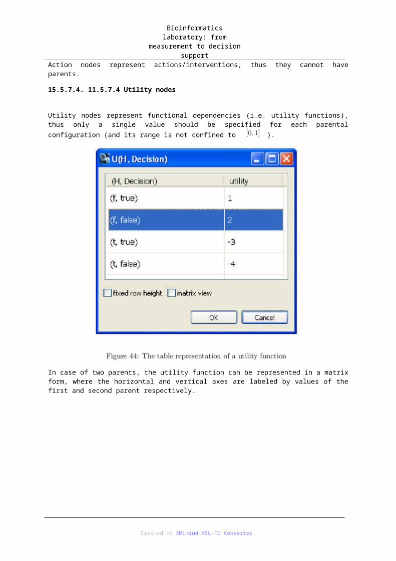
Bioinformatics laboratory: from measurement to decision support
ecalibacterium(100);Otu005 264 Bacteria(100);Firmicutes(96);Negativicutes(92);Selenomonadales(92);Veillonellaceae(92);Anaeroglobus(92);
Note that the same genus level can be assigned to different OTUs. This indicates that these OTUs represent sub-OTU lineages.
For the further processing steps, we need to determine the OTU composition of each sample by parsing the stool.final.an.list file with the make.shared command:
make.shared(list=stool.final.an.list, group=stool.final.groups, label=0.03)
which creates 8 rabund files (one for each of the 8 samples) and a shared file. Check this shared file (stool.final.an.shared) in a text editor.
21.3.2. 14.3.2 Alpha-diversity
Now, we are ready to address our original questions. We begin with analyzing the alpha-diversity of our samples. Remember that the structure of the community (i.e. the diversity) depends on the number of the different species (also denoted as richness) and their relative abundances (also denoted as evenness).
First, let us plot the rank-abundance curve of each sample (see Figure 57). Remember that a rank-abundance curve characterizes the unevenness of the community by plotting the relative abundances of the operational taxonomic units. The relative abundances are stored in the rabund files (stool.final.an.F*Fcsw.rabund).
Measuring the species richness might first seem an easy task: just count the number of different species in the environment. However, as we are sampling from the environment, there might be species that we did not observe and therefore our guess would be an underestimate of the true richness. The process of counting the observed species by the number of sampled individuals (i.e. the number of read sequences) can be depicted as a species accumulation curve. Richness then can be approximated by extrapolating the curve to estimate its
Created by XMLmind XSL-FO Converter.
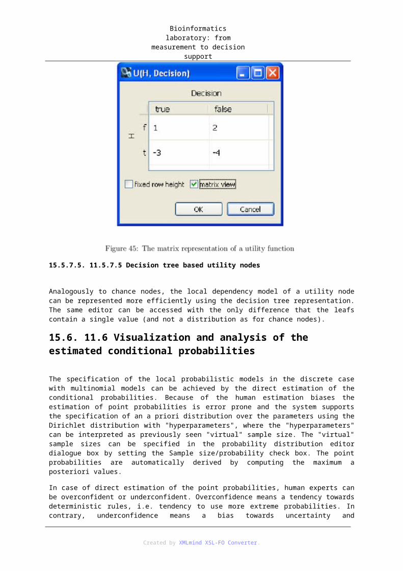
Bioinformatics laboratory: from measurement to decision support
unknown asymptote.
To plot a smoothed version of a species accumulation curve, called a rarefaction curve, we randomly select (with replacement) , , ..., reads from the full set of reads, estimate how many species we found based on the selected reads, and plot the mean of many such draws (see Figure 58). If the curve flattens, this means that we discover fewer and fewer new species, so by sequencing more, we probably won't find many more species. On the contrary, if the curve does not flatten, this means that we have not sequenced enough.
We can calculate the rarefaction curve with the rarefaction.single command:
mothur > rarefaction.single(shared=stool.final.an.shared, freq=10)
This creates a file, named stool.final.an.groups.rarefaction, that contains the rarified number of OTUs in every 10 sequences for each sample. Use your favorite software to plot these results (see Figure 58).
Beside the rarefaction curves, there are non-parametric richness estimators, from which the simplest is Chao1, calculated as follows:
where is the number of observed species, and it is augmented by a term calculated from the observed number of singletons ( , number of species represented by only one read) and doubletons ( , number of species represented by two reads). The main advantage of using nonparametric richness estimators, like Chao1, is that they are able to approximate true richness from fewer sequences than rarefaction curves [53].
Besides species richness, relative abundance is also important to assess the complexity of a community. For example, a community in which many different species appear in closely equal abundance is more complex than a community with less species, or a community with unequal abundance. A community is simple if only a few species dominate the environment and the other species are very rare.
Diversity measures that encompass evenness are somewhat more sophisticated than previous measures [54 és 53]. The most commonly used are Shannon diversity index
Created by XMLmind XSL-FO Converter.

Bioinformatics laboratory: from measurement to decision support
and Simpson index
where is the total number of different species, and is the relative abundance of species in the sample. The Shannon diversity index (or Shannon entropy) quantifies the entropy in community composition: the more different species there are in the community and the more even their relative abundance is, the more difficult it is to correctly predict which species a randomly chosen sequence will originate from. This measure quantifies the uncertainty of this prediction. Simpson index is similar, but less sensitive to richness and more sensitive to evenness than Shannon diversity. Simpson index equals the probability that two randomly chosen reads originate from the same species.
We can generate the value of the estimators and diversity indices with the collect.single command:
mothur > collect.single(shared=stool.final.an.shared, calc=chao-shannon-simpson, freq=10)
which creates a file with a table for every sample and for every calculator. Let us plot these results (see Figure 59).
21.3.3. 14.3.3 Beta-diversity
Created by XMLmind XSL-FO Converter.

Bioinformatics laboratory: from measurement to decision support
In the next step, we compare the eight gut microbial communities based on their membership and community structure. This corresponds to analyzing the beta-diversity of the samples (i.e. the difference in diversity associated with differences in habitat [53]).
We begin with visualizing the distances of the samples based on their community composition. First, we calculate the distances with the dist.shared command, and then calculate the principal coordinates with the pcoa command:
mothur > dist.shared(shared=stool.final.an.shared, calc=jclass)
mothur > pcoa(phylip=stool.final.an.jclass.0.03.lt.dist)
The dissimilarity of the communities is calculated by the Jaccard index:
where is the number of shared OTUs between the two communities, and is the number of OTUs in the first, and the second community, respectively.
Let us plot the result of the Principal Coordinate Analysis (see Figure 60). The pcoa commands creates a .loading file which describes the fraction of the total variance in the data represented by each of the axes. The variance explained by the first three axes sums up to . The .axes file created by the pcoa command describes the position of each sample in the PCoA plot. It can be clearly seen that the first axis clearly separates the two individuals from each other.
To determine which OTUs are differentially represented between the two individuals, we can use a statistical test implemented in the metastats command [55]. First, we create a file which describes which sample comes from which individual (see stool.design). This is called a design file, because it describes the design of our experiment. Next, we call metastats:
mothur > metastats(shared=stool.final.an.shared, design=stool.design)
which creates a .metastats file that lists all OTUs and the corresponding p and q value (the false positive rate and the false discovery rate, respectively) which tell whether the specific OTU is overrepresented in one of the two samples.
Created by XMLmind XSL-FO Converter.

Bioinformatics laboratory: from measurement to decision support
21.4. 14.4 Questions
1. Explain the main steps of a 16S rRNA based metagenomic analysis.
2. Explain the method of taxonomic classification by RDP.
3. What is an Operational Taxonomic Unit (OTU)?
4. What is Alpha-diversity?
5. What is a rank-abundance curve?
6. What is a species accumulation curve and what is a rarefaction curve? Explain the differences between them.
7. Define the Shannon diversity index and the Simpson diversity index. Explain their intuitive interpretation.
8. What is Beta-diversity?
22. References
• [51] Elizabeth K. Costello, Christian L. Lauber, Micah Hamady, Noah Fierer, Jeffrey I. Gordon, and Rob Knight. Bacterial community variation in human body habitats across space and time. Science, 326(5960):1694-1697, December 2009.
• [52] Patrick D. Schloss, Sarah L. Westcott, Thomas Ryabin, Justine R. Hall, Martin Hartmann, Emily B. Hollister, Ryan A. Lesniewski, Brian B. Oakley, Donovan H. Parks, Courtney J. Robinson, Jason W. Sahl, Blaz Stres, Gerhard G. Thallinger, David J. Van Horn, and Carolyn F. Weber. Introducing mothur: open-source, platform-independent, community-supported software for describing and comparing microbial communities. Applied and environmental microbiology, 75(23):7537-7541, December 2009. PMID: 19801464.
• [53] Simon A. Levin, Stephen R. Carpenter, H. Charles J. Godfray, Ann P. Kinzig, Michel Loreau, Jonathan B. Losos, Brian Walker, and David S. Wilcove, editors. The Princeton Guide to Ecology. Princeton University Press, September 2012.
• [54] Tom C. J. Hill, Kerry A. Walsh, James A. Harris, and Bruce F. Moffett. Using ecological diversity measures with bacterial communities. FEMS microbiology ecology, 43(1):1-11, February 2003. PMID: 19719691.
• [55] James Robert White, Niranjan Nagarajan, and Mihai Pop. Statistical methods for detecting differentially abundant features in clinical metagenomic samples. PLoS Comput Biol, 5(4):e1000352, April 2009.
Created by XMLmind XSL-FO Converter.