Reframing the magnetotelluric phase tensor formonitoring applications: improved accuracy andprecision in strike determinationsAna Gabriela Bravo-Osuna  ( abravo@cicese.edu.mx )

Centro de Investigacion Cienti�ca y de Educacion Superior de Ensenada https://orcid.org/0000-0002-6848-2806Enrique Gómez-Treviño 

Centro de Investigacion Cienti�ca y de Educacion Superior de EnsenadaOlaf Josafat Cortés-Arroyo 

Bundesanstalt für Geowissenschaften und Rohstoffe (BGR)Néstor Fernando Delgadillo-Jáuregui 

Centro de Investigacion Cienti�ca y de Educacion Superior de EnsenadaRocío Fabiola Arellano-Castro 

Centro de Investigacion Cienti�ca y de Educacion Superior de Ensenada

Full paper

Keywords: Magnetotelluric monitoring, Phase tensor, Swift strike, Galvanic distortion

Posted Date: August 28th, 2020

DOI: https://doi.org/10.21203/rs.3.rs-23277/v2

License: This work is licensed under a Creative Commons Attribution 4.0 International License.  Read Full License

Version of Record: A version of this preprint was published on February 2nd, 2021. See the publishedversion at https://doi.org/10.1186/s40623-021-01354-y.

1

Reframing the magnetotelluric phase tensor for

monitoring applications: improved accuracy and

precision in strike determinations

Ana G. Bravo-Osuna1, Enrique Gómez-Treviño1, Olaf J. Cortés-Arroyo1,2, Nestor

F. Delgadillo-Jauregui1and Rocío F. Arellano-Castro1

1 Departamento de Geofísica Aplicada, División de Ciencias de la Tierra,

CICESE, Ensenada, Baja California, México. 22860.

2 Presently at Federal Institute for Geosciences and Natural Resources (BGR),

Berlin, Germany.

ABSTRACT

The magnetotelluric method is increasingly being used to monitor electrical

resistivity changes in the subsurface. One of the preferred parameters derived

from the surface impedance is the strike direction, which is very sensitive to

changes in the direction of the subsurface electrical current flow. The preferred

method for estimating the strike changes is that provided by the phase tensor

because it is immune to galvanic distortions. However, it is also a fact that the

associated analytic formula is unstable for noisy data, something that limits its

applicability for monitoring purposes, because in general this involves

comparison of two or more very similar data sets. On the other hand, the

classical Swift’s approach for strike is very stable for noisy data but it is severely

Correspondence to: Ana G. Bravo-Osuna

División Ciencias de la Tierra, Centro de Investigación Científica y de Educación Superior de Ensenada. Baja California, México, 22860. e-mail: abravo@cicese.edu.mx

2

affected by galvanic distortions. In this paper we impose the criterion of Swift’s

approach to the phase tensor. Rather than developing an analytical formula we

optimize numerically the same criterion. This stabilizes the estimation of strike by

relaxing an exact condition to an optimal condition in the presence of noise. This

has the added benefit that it can be applied to windows of several periods, thus

providing tradeoffs between variance and resolution. The performance of the

proposed approach is illustrated by its application to synthetic data and to real

data from a monitoring array in the Cerro Prieto geothermal field, México.

Keywords: Magnetotelluric monitoring Phase tensor Swift strike

Galvanic distortion

3

INTRODUCTION

The evolution of the magnetotelluric (MT) method, from its scalar to its

tensorial version, brought about issues regarding the best ways to process the

impedance tensor to obtain information about the subsurface. In many instances

what is required is to identify the directionality of the electric currents because

this is related to lateral changes in electrical resistivity. In the case of two-

dimensional (2D) models this translates into finding the strike angle for which the

measured tensor reduces in some manner to a special case. When one of the

axes of the coordinate system is parallel to the strike, the diagonal elements of

the impedance tensor are zeroes. Swift’s (1967) approach to find the appropriate

angle is to assume a rotated version of the measured tensor, which in general is

not aligned along strike, and then look for the angle that best fits the 2D criterion.

The approach leads to an analytical formula. Another analytic formula that

converts the elements of the impedance tensor into a strike angle was developed

by Bahr (1988) by imposing the condition that the elements of the columns of the

impedance tensor must have the same phases in the case of 2D structures.

Groom and Bailey (1989) proposed an approach that numerically fits, in a least

square sense, the measured impedances with an appropriate model that

includes the strike angle. In this case the solution is not an analytic formula.

Finally, there is the phase tensor of Caldwell et al. (2004) from which an analytic

formula is derived for the strike angle.

4

The approaches described above for strike determinations differ from each

other in several ways, and are also similar in other ways. Let us consider first the

similarities between Bahr’s and the phase tensor approaches. Both are devised

with the explicit purpose in mind of avoiding the effect of galvanic distortions.

Also, they impose rigorous criteria in the sense that, strictly speaking, they can

be met only by error-free data. A third similarity is that in both cases the

approaches lead to analytic formulae. Let us now consider the similarities

between the Swift’s and Groom-Bailey’s approaches. Both impose somewhat

relaxed criteria as opposed to the exact requirements in the other two options.

Instead of an exact fit a best fit is sought in the least squares sense. In Swift’s

case, the anti-diagonal elements are not forced to be exactly zeroes but only to

have their minimum possible amplitude. The Groom-Bailey approach also

complies with a least squares criterion.

In the case of error-free data all approaches cannot but produce the same

result. However, in the case of data with errors the least squares criterion

provides a balanced solution by design, by acknowledging from the begining the

possibility of inconsistencies. Our hypothesis is that imposing the least squares

criterion on the phase tensor determination of strike will improve the performance

of the analytic formula.

Presently it is almost a requirement to include phase tensor ellipses as

part of the interpretation of any data set. Usually they are drawn over maps of the

study area to reveal directionality of shallow or deep structures depending on the

period of interest (e.g. Martí et al., 2020; Comeau et al., 2020). It is not

5

uncommon for the axes of the ellipses to point in inconsistent directions because

of random noise. Any improvement in this respect would be certainly welcome.

However, where better determinations of strikes are most needed is in the recent

application of the magnetotelluric method in monitoring applications. The

preferred formula for monitoring purposes is that derived from the phase tensor

(e.g. Peacock et al. 2012; 2013). One of the reasons is that there is no

assumption about dimensionality. All other approaches assume 2D structures.

Another reason is that it is immune to galvanic distortions, something that Swift’s

formula is not. However, its drawback is that it is unstable for noisy data (Jones,

2012). This limits its applicability for monitoring purposes to very precise data, to

ensure a precise estimation of strike. The question then arises of whether we can

improve the estimation of strikes beyond the application of the analytic formula.

All the analytic formulae provide strike estimates period by period. That is, each

estimate and its variance are independent from the others. However, it is

possible to link contiguous periods by assuming smooth variations of strike over

period and produce a stable profile in the manner of the Occam philosophy (e.g.

Constable et al., 1987). Muñiz et al. (2017) explored this path for the phase

tensor using as seeds the estimations that are better constrained. Another

possibility for stabilization is exemplified by the Groom-Bailey approach as

generalized by McNeice and Jones (2001); the estimates can be made period by

period, for a given number of periods or for all periods together. The variance of

the estimates generally diminishes as the number of periods increases. In a way,

this follows the philosophy of Backus and Gilbert (1968) in the sense that the

6

variance can be improved at the cost of resolution. In this paper we adhere to

this viewpoint and look for estimates that can be made period by period, for a

given number of periods, or for all periods at the same time.

THEORY

Phase tensor

The history of the magnetotelluric method is plentiful of examples where

the problem to be solved consists of avoiding something undesirable. For

instance, consider the chaotic variations of the source strength when making

telluric measurements. The variations were neutralized by the inclusion of the

magnetic field into the telluric method (Cagniard, 1953). In turn, the also chaotic

polarizations of the source were taken care of by the impedance tensor

(Cantwell, T., 1960). The not less chaotic distribution of small, near surface

heterogeneities that produce galvanic distortions was neutralized by the phase

tensor (Caldwell et al., 2004). The present work also centers on an avoidance. In

this case, mitigate the effect of random noise in the estimations of strike using

the phase tensor.

Let us start by a brief account of the development of the phase tensor

itself. In relation to distortions, small, near surface heterogeneities means that

depth, size and distance to the electric line must be smaller than the skin depth.

All things considered, local electromagnetic induction is small so that only

galvanic effects due to electric charges are important. Physically, the source of

7

the charges is the undistorted electric field, so their strength must be proportional

to the strength of the source. In short, that the measured or distorted electric

field𝑬! can be modeled as 𝑬! = 𝑪𝑬,where 𝑪 is a distortion matrix and 𝑬 is the

undistorted electric field. In terms of 𝑥 and 𝑦 components

(𝐸"!𝐸#!* = (𝐶$$ 𝐶$%𝐶%$ 𝐶%%* (𝐸"𝐸#*.(1)

The elements of the distortion matrix 𝑪 are real on behalf of the large skin-

depth assumption. The charges are in phase and follow the undistorted electric

field. The diagonal elements account for the distortion produced by a component

to the same the component, while the off diagonal for the orthogonal

contributions. To see how the distorted electric fields affect the impedance

tensor, consider the undistorted fields expressed in terms of the impedances

(𝐸"𝐸#* = (𝑍"" 𝑍"#𝑍#" 𝑍##* (

𝐻𝑥𝐻𝑦*,(2)

where 𝐻" and 𝐻# are the corresponding components of the magnetic field and 𝑍&' represents the elements of the impedance tensor. The distorted impedance

tensor can be written as

(𝑍""! 𝑍"#!𝑍#"! 𝑍##!* = (𝐶$$ 𝐶$%𝐶%% 𝐶%%* (

𝑍"" 𝑍"#𝑍#" 𝑍##*(3)

8

The real elements of the distortion matrix affect only the amplitude of the

impedances, but this is solely for the individual products. The actual linear

combination can produce distorted impedances that resemble none of the

originals. This explains the importance of the subject and the attempts to

neutralize the effects of the distortion matrix. The formula developed by Bahr

(1988) for the strike of 2D structures might be considered a precursor to the more

general formula derived from the phase tensor. It happens that for the strike

angle the product of the distortion matrix and the impedance tensor has a special

property: the elements of each column must have the same phase. Imposing

this condition on the measured impedance Bahr (1988) developed his formula for

the strike which holds regardless of the distortion matrix. The phase tensor of

Caldwell et al. (2004) generalizes this formula and provides other parameters

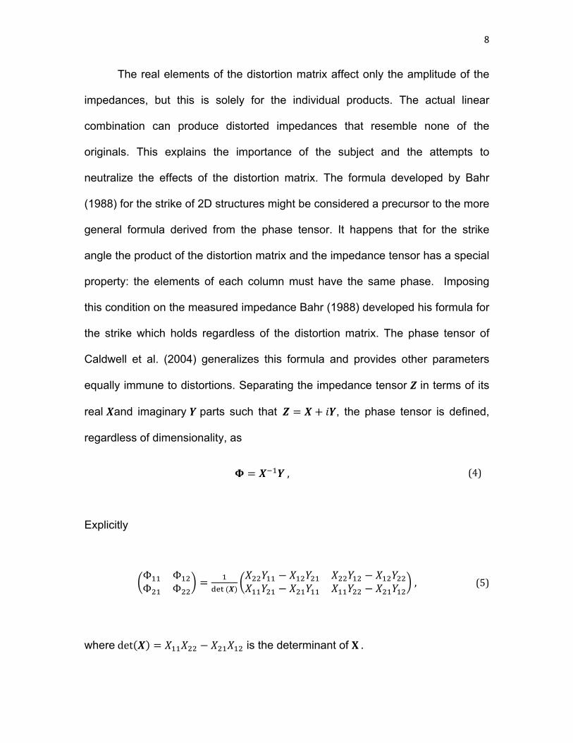
equally immune to distortions. Separating the impedance tensor 𝒁 in terms of its

real 𝑿and imaginary 𝒀 parts such that 𝒁 = 𝑿 + 𝑖𝒀, the phase tensor is defined,

regardless of dimensionality, as

𝚽 = 𝑿($𝒀, (4)

Explicitly

(Φ$$ Φ$%Φ%$ Φ%%* = $

)*+(𝑿)(𝑋%%𝑌$$ − 𝑋$%𝑌%$ 𝑋%%𝑌$% − 𝑋$%𝑌%%𝑋$$𝑌%$ − 𝑋%$𝑌$$ 𝑋$$𝑌%% − 𝑋%$𝑌$%*,(5)

wheredet(𝑿) = 𝑋$$𝑋%% − 𝑋%$𝑋$% is the determinant of X.

9

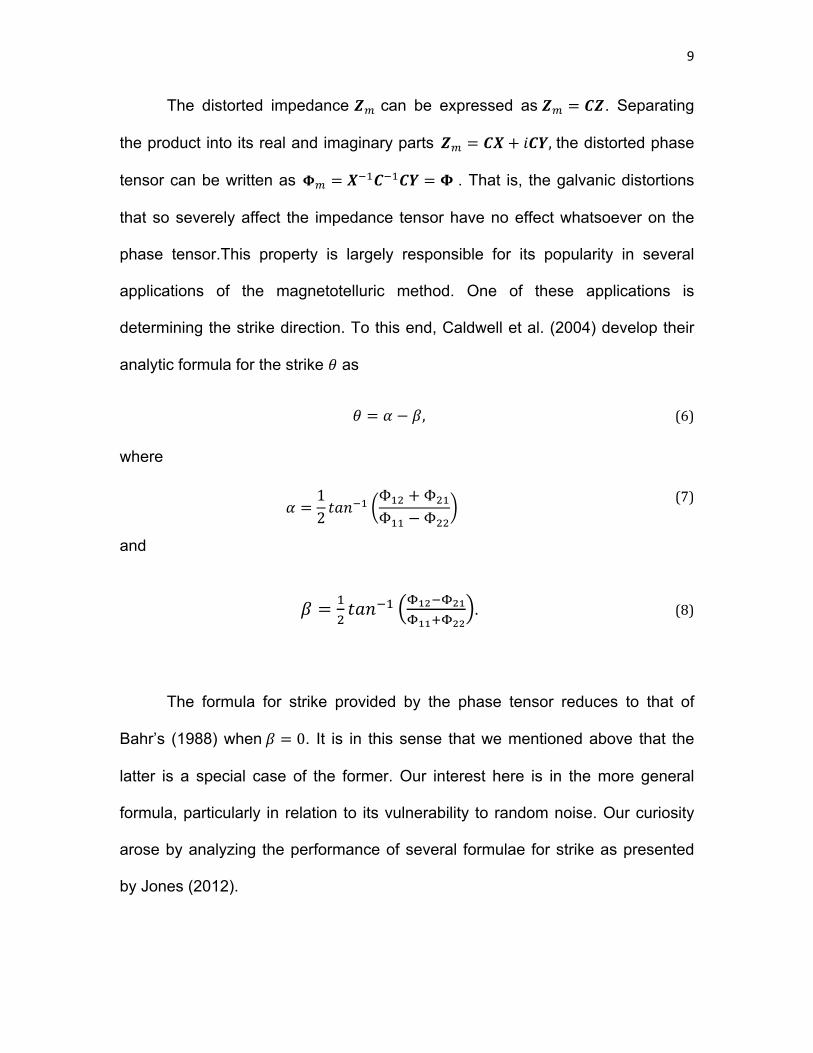
The distorted impedance 𝒁! can be expressed as𝒁! = 𝑪𝒁. Separating

the product into its real and imaginary parts𝒁! = 𝑪𝑿 + 𝑖𝑪𝒀, the distorted phase

tensor can be written as𝚽! = 𝑿($𝑪($𝑪𝒀 = 𝚽 . That is, the galvanic distortions

that so severely affect the impedance tensor have no effect whatsoever on the

phase tensor.This property is largely responsible for its popularity in several

applications of the magnetotelluric method. One of these applications is

determining the strike direction. To this end, Caldwell et al. (2004) develop their

analytic formula for the strike 𝜃 as

𝜃 = 𝛼 − 𝛽,(6)

where

𝛼 = 12 𝑡𝑎𝑛

($ (Φ$% +Φ%$

Φ$$ −Φ%%

* and

(7)

𝛽 = !

"𝑡𝑎𝑛#! &$#$#$$#

$##%$$$

'.(8)

The formula for strike provided by the phase tensor reduces to that of

Bahr’s (1988) when𝛽 = 0. It is in this sense that we mentioned above that the

latter is a special case of the former. Our interest here is in the more general

formula, particularly in relation to its vulnerability to random noise. Our curiosity

arose by analyzing the performance of several formulae for strike as presented

by Jones (2012).

10

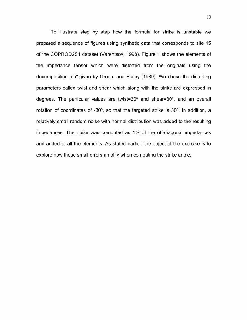
To illustrate step by step how the formula for strike is unstable we

prepared a sequence of figures using synthetic data that corresponds to site 15

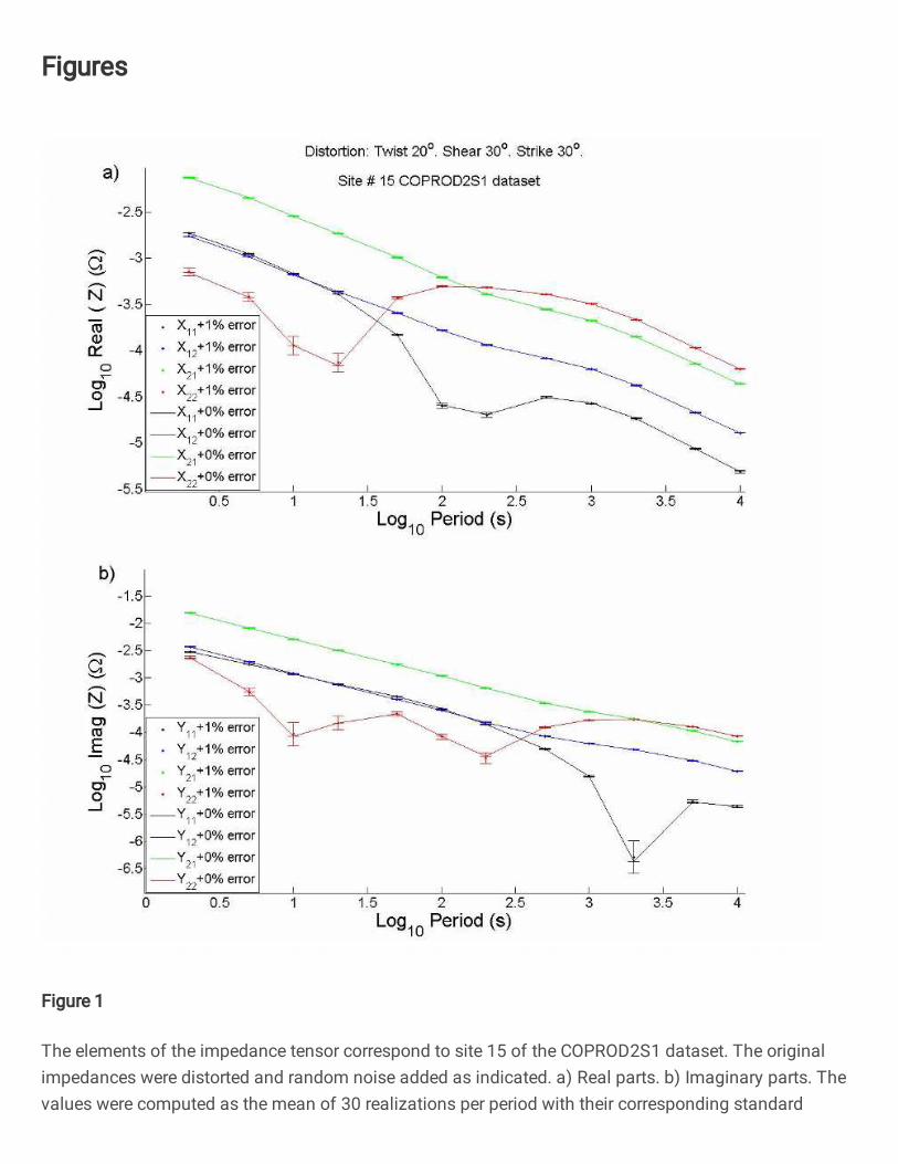
of the COPROD2S1 dataset (Varentsov, 1998). Figure 1 shows the elements of

the impedance tensor which were distorted from the originals using the

decomposition of 𝑪 given by Groom and Bailey (1989). We chose the distorting

parameters called twist and shear which along with the strike are expressed in

degrees. The particular values are twist=20o and shear=30o, and an overall

rotation of coordinates of -30o, so that the targeted strike is 30o. In addition, a

relatively small random noise with normal distribution was added to the resulting

impedances. The noise was computed as 1% of the off-diagonal impedances

and added to all the elements. As stated earlier, the object of the exercise is to

explore how these small errors amplify when computing the strike angle.

11

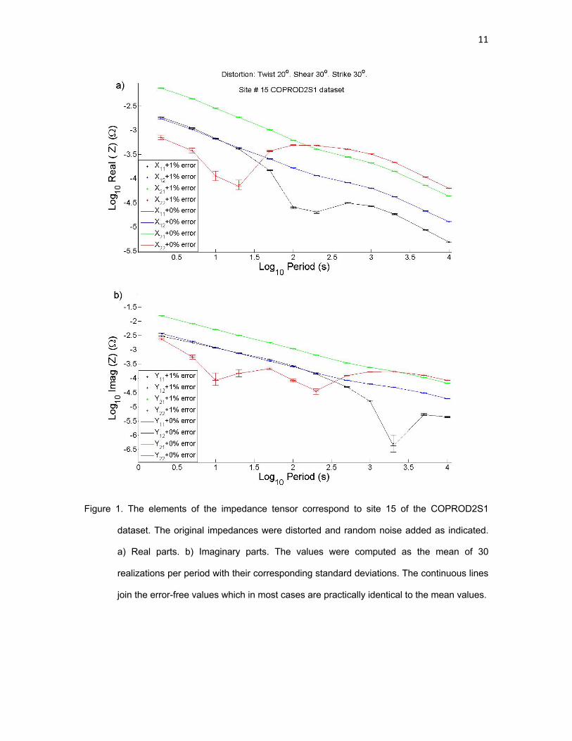
Figure 1. The elements of the impedance tensor correspond to site 15 of the COPROD2S1

dataset. The original impedances were distorted and random noise added as indicated.

a) Real parts. b) Imaginary parts. The values were computed as the mean of 30

realizations per period with their corresponding standard deviations. The continuous lines

join the error-free values which in most cases are practically identical to the mean values.

12

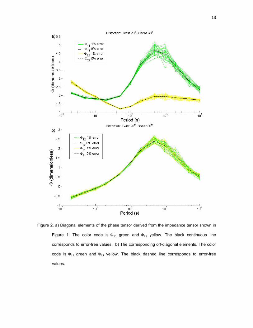
The first level of computations involves using the impedances in the

formula for the phase tensor given by equation 5. The computed diagonal

elements are shown in Figure 2a, where it can be observed that they are almost

error-free for the first six periods and are noisier for the last six. The off-diagonal

elements shown in Figure 2b behave very much the same. Notice that for the first

six periods the elements are equal, indicating that the tensor is symmetric. In

fact, they should be equal for all periods because the data were drawn from a 2D

model. The fact that they are not for the last six periods is due entirely to the

noise and to the distortions which introduce 3D effects.

13

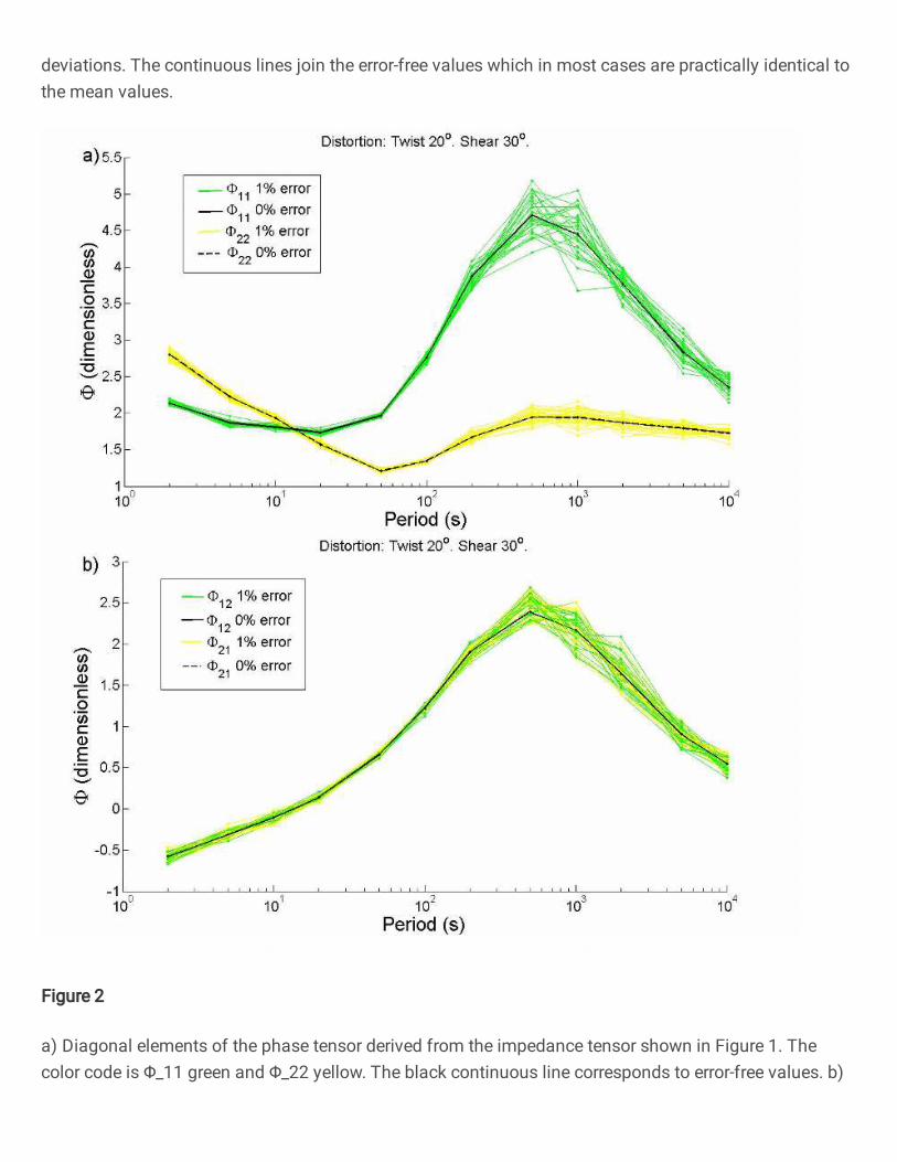
Figure 2. a) Diagonal elements of the phase tensor derived from the impedance tensor shown in

Figure 1. The color code is Φ!! green and Φ"" yellow. The black continuous line

corresponds to error-free values. b) The corresponding off-diagonal elements. The color

code is Φ!" green and Φ"! yellow. The black dashed line corresponds to error-free

values.

14

We now turn to the ratios that define the angles 𝛼 and 𝛽 . The former

involves the sum of the off-diagonal elements as numerator and the subtraction

of the diagonal elements as denominator. Notice in Figure 3a that both quantities

go through zero at a period of about 10 s. This will have implications when

computing the ratio. Figure 3b illustrates the variations of the sum of the diagonal

and the subtraction of the off-diagonal elements. This subtraction falls around

zero for all periods, but no problem is expected when taking the ratio because for

the angle 𝛽 the subtraction goes into the numerator. Notice that for the last six

periods the subtraction has less scattering than the individual elements shown in

Figure 2b.

15

Figure 3. a) Combination of the phase tensor elements that make up the ratio in the formula for

the angle 𝛼 . The color code is Φ!! − Φ"" green and Φ!" + Φ"! yellow. The black

continuous line corresponds to error-free values. b) Corresponding combination for the

angle𝛽. The color code isΦ!! + Φ"" green andΦ!" − Φ"! yellow. The black dashed

line corresponds to error-free values.

16

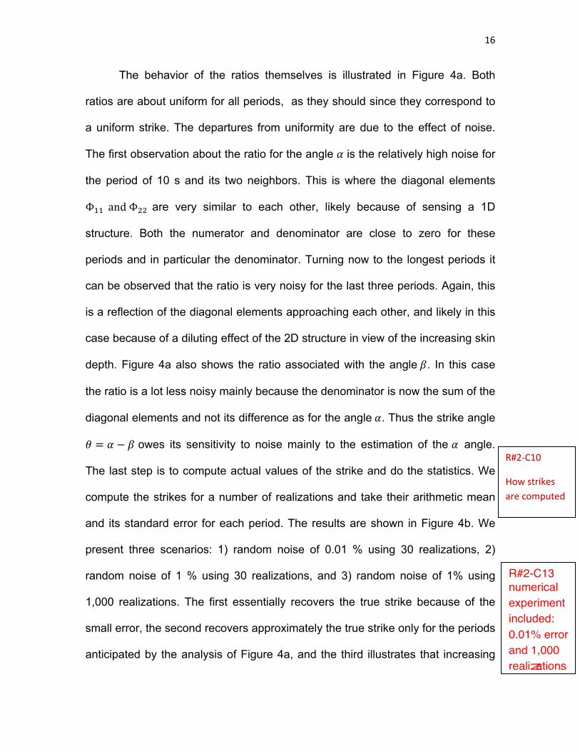
The behavior of the ratios themselves is illustrated in Figure 4a. Both

ratios are about uniform for all periods, as they should since they correspond to

a uniform strike. The departures from uniformity are due to the effect of noise.

The first observation about the ratio for the angle 𝛼 is the relatively high noise for

the period of 10 s and its two neighbors. This is where the diagonal elements

Φ$$andΦ%% are very similar to each other, likely because of sensing a 1D

structure. Both the numerator and denominator are close to zero for these

periods and in particular the denominator. Turning now to the longest periods it

can be observed that the ratio is very noisy for the last three periods. Again, this

is a reflection of the diagonal elements approaching each other, and likely in this

case because of a diluting effect of the 2D structure in view of the increasing skin

depth. Figure 4a also shows the ratio associated with the angle𝛽. In this case

the ratio is a lot less noisy mainly because the denominator is now the sum of the

diagonal elements and not its difference as for the angle𝛼. Thus the strike angle

𝜃 = 𝛼 − 𝛽 owes its sensitivity to noise mainly to the estimation of the 𝛼 angle.

The last step is to compute actual values of the strike and do the statistics. We

compute the strikes for a number of realizations and take their arithmetic mean

and its standard error for each period. The results are shown in Figure 4b. We

present three scenarios: 1) random noise of 0.01 % using 30 realizations, 2)

random noise of 1 % using 30 realizations, and 3) random noise of 1% using

1,000 realizations. The first essentially recovers the true strike because of the

small error, the second recovers approximately the true strike only for the periods

anticipated by the analysis of Figure 4a, and the third illustrates that increasing

R#2-C13

numerical

experiment

included:

0.01% error

and 1,000

realizations

R#2-C10

How strikes

are computed

17

the number of realizations improves both accuracy and precision. However, one

cannot but notice that for the period of 10 s the strike is underestimated in spite

of the small error and the 1000 realizations. This point deserves further attention

because it may be the tip of the iceberg of something deeper, in view that the

ratios and the trigonometric function tangent are nonlinear combinations of the

data and thus not easy to visualize.

.

18

Figure 4. a) The ratios that make up the formulae for the angles 𝛼 and𝛽. The color code is green

for the angle 𝛼 and yellow for the angle𝛽. The black continuous line corresponds to error-

free values. b) The final results for the strike 𝜃 = 𝛼 − 𝛽. The red line corresponds to

estimates assuming 1% error and using 30 realizations. The black line corresponds to 1%

error and 1000 realizations. The dashed blue line corresponds to 0.01% error and 30

realizations.

It is difficult just by inspection to predict the outcomes of a nonlinear

formula. Consider for instance Figure 4a. There is a bias towards higher values

for some of the realizations around the period of 10 s. One would think that

increasing the number of realizations would simply fill out the empty spaces. In

fact, this is what happens except for a small but significant difference. Figure 5a

presents the estimates for the same 1 % error and 1000 realizations. It can be

observed how some realizations are consistently negative for the period of 10 s.

These values seem isolated outliers but actually they are not. Figure 5a also

presents the case of 5 % error which illustrates that this is a systematic effect

associated with how the strike is computed. In most of the examples that follow

we use 5 % error and 30 realizations, which we consider are appropriate to

illustrate the main point of this work. At this level of error the results of using 30

or 1,000 realizations are comparable as illustrated in Figure 5b.

19

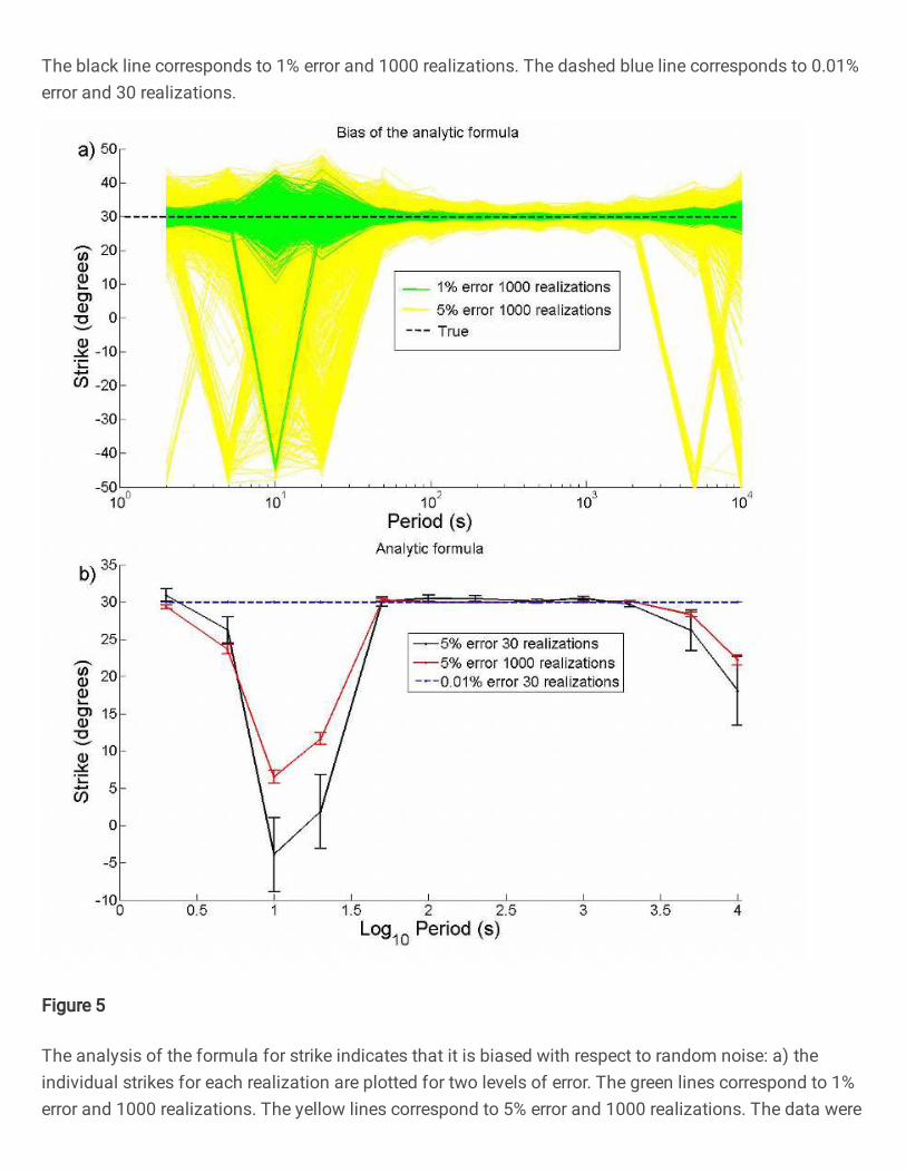
Figure 5. The analysis of the formula for strike indicates that it is biased with respect to random

noise: a) the individual strikes for each realization are plotted for two levels of error. The

green lines correspond to 1% error and 1000 realizations. The yellow lines correspond to

5% error and 1000 realizations. The data were distorted assuming twist= 20o and shear

=30o. The dashed line represents the true strike as computed with 0.01 % error. b) The

black line represents the estimates of strikes using 5 % error and 30 realizations. The red

line represents the estimates using 5 % error and 1,000 realizations

20

The overall analysis in this section applies only to site 15 of the

COPROD2S1 data set. It does not pretend to be a general proof that one ratio or

the other is most sensitive to random noise. We see it as a window into what is

behind the unstable character of the formula for strike based on the phase

tensor. However, more than just an analysis of what is happening, the objective

is to devise, based on this diagnostic, a way to lessen the effect of random noise

on the determination of strike. This is addressed in the next section. The

challenge is to go beyond a simple approach of just taking moving averages of

the estimates from the formula, and somehow jump over the nonlinear character

of the whole process.

Reframing the phase tensor

Let us begin by recalling two steps taken by Swift (1967) in developing his

now almost forgotten formula for strike. The first thing is to consider a rotated

version of the impedance tensor

$Z%%

& Z%'&Z'%& Z''& & = 𝐑(θ)𝐙𝐑)(θ).(9)

The second step is to solve for the strike angle using a least squares criterion.

That is, finding𝜃 that minimizes

𝐶0#(𝜃) = I𝑍$$′ (𝜃)I% + I𝑍%%′ (𝜃)I%. (10)

21

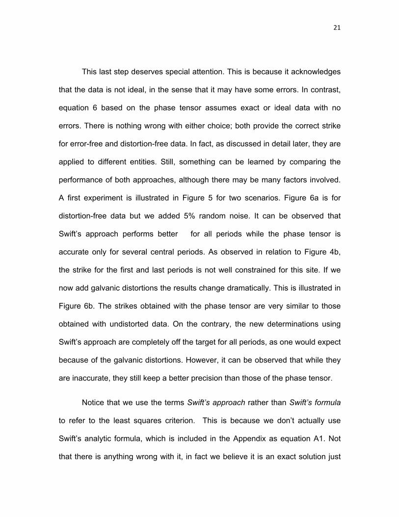
This last step deserves special attention. This is because it acknowledges

that the data is not ideal, in the sense that it may have some errors. In contrast,

equation 6 based on the phase tensor assumes exact or ideal data with no

errors. There is nothing wrong with either choice; both provide the correct strike

for error-free and distortion-free data. In fact, as discussed in detail later, they are

applied to different entities. Still, something can be learned by comparing the

performance of both approaches, although there may be many factors involved.

A first experiment is illustrated in Figure 5 for two scenarios. Figure 6a is for

distortion-free data but we added 5% random noise. It can be observed that

Swift’s approach performs better for all periods while the phase tensor is

accurate only for several central periods. As observed in relation to Figure 4b,

the strike for the first and last periods is not well constrained for this site. If we

now add galvanic distortions the results change dramatically. This is illustrated in

Figure 6b. The strikes obtained with the phase tensor are very similar to those

obtained with undistorted data. On the contrary, the new determinations using

Swift’s approach are completely off the target for all periods, as one would expect

because of the galvanic distortions. However, it can be observed that while they

are inaccurate, they still keep a better precision than those of the phase tensor.

Notice that we use the terms Swift’s approach rather than Swift’s formula

to refer to the least squares criterion. This is because we don’t actually use

Swift’s analytic formula, which is included in the Appendix as equation A1. Not

that there is anything wrong with it, in fact we believe it is an exact solution just

22

as the one derived from the phase tensor. What we do is to sample numerically

the strike every one degree and then select the minimum of the penalty function.

The issue is treated with more detail in the Appendix since this is peripheral to

the subject matter.

One of the differences between the two approaches is that the conditions

imposed on the elements of the corresponding tensors are applied to quantities

of different order. Swift’s approach operates directly on the elements of the

impedance tensor. On the other hand, the condition imposed on the phase tensor

is applied to combinations of ratios of the impedances. If this is the only reason

for the poor performance of the phase tensor, then there is nothing to do to

improve it. This is because it is precisely the use of those ratios that make the

phase tensor immune to galvanic distortions. This is an asset nobody is willing to

dispose of. The only viable alternative for improvement is to keep as much as

possible the assets of the phase tensor, and somehow import from Swift’s

approach the least squares criterion.

23

Figure 6. Determination of strike angles using the phase tensor and Swift’s approach: a) with no

galvanic distortions. The black dashed line represents the true strike. The black

continuous line represents the estimates using Swift’s least squares approach applied to

the elements of the impedance tensor. The red line corresponds to the estimates using

the analytic formula derived from the phase tensor. b) With galvanic distortions. The

black dashed line represents the true strike. The black continuous line represents the

estimates using Swift’s least squares approach applied to the elements of the impedance

24

tensor. The red line corresponds to the estimates using the analytic formula derived from

the phase tensor.

Our approach relies, of course, on the theory behind the phase tensor of

Caldwell et al. (2004), who factorize the phase tensor as

𝚽 = 𝐑)(α − β) $Φ*+, 00 Φ*-.

&𝐑(α + β),(11)

where𝛼 − 𝛽and𝐑are the strike angle and the rotation matrix, respectively. Φ123

and Φ145 are the singular values of the phase tensor. Notice that the rotation on

the left is for the difference of the angles and that that on the right is for the sum

of them. To make this product symmetric multiply on the right by 𝐑(2β) so that

𝚽 = 𝐑𝐓(α − β) $Φ*+, 00 Φ*-.

&𝐑(α − β)𝐑(2β).(12)

We now solve for the matrix of eigenvalues as

$Φ*+, 00 Φ*-.

& = 𝐑(𝛼 − 𝛽)𝚽𝐑0𝟏(2β)𝐑)(𝛼 − 𝛽).(13)

Assuming that the strike 𝜃 = 𝛼 − 𝛽 is an unknown, the matrix of singular or

principal values is no longer diagonal unless it corresponds to the appropriate

strike. In general

$Φ%%& Φ%'

&

Φ'%& Φ''

& & = 𝐑(θ)𝚽𝐑0𝟏(2β)𝐑)(θ).(14)

25

Posed in these terms, the analytic formula for strike obtained by Caldwell et al.

(2004) would correspond to setting Φ$%′ = Φ%$

′ = 0. Using Swift’s criterion this

would correspond to minimize

𝐶0#(𝜃) = Φ$%6 (T4, θ)% +Φ%$

6 (T4, θ)%.(15)

In other words, for every periodT4, we would look for the angle 𝜃 that minimizes

the size of the anti-diagonal elements of the phase tensor as defined by equation

(14), instead of imposing the condition that they must be exactly zeroes. To

compute the angle 𝛽 we use equation 8, so the optimization of 𝜃 = 𝛼 − 𝛽 is made

under this assumption. This we call reframing the phase tensor for strike

determinations. In practice the penalty function is sampled every one degree in

the range 07 ≤ 𝜃 ≤ 907 . In principle, the domain of potential strikes should

include negative angles. However, this is not necessary because we are still

working within the classical 907 ambiguity, as are all methods for determining

strikes. In other words, a given angle 𝜃 has a 𝜃 − 907companion as possible

solution for the strike. Under this assumption, the performance of the approach is

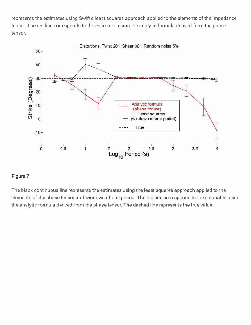
compared with that of the analytic formula in Figure 7 for a target strike of307. It

can be observed that there is a definite gain in using the least squares criterion

over that of the exact analytic formula. In this case we used 5 % random error

and 30 realizations as for Figure 5, and again the estimates behave similarly with

some outliers from the analytic formula. The least squares approach lessens this

effect except for two of the first periods. However, the improvement does not

match the better performance of Swift’s approach seen in Figure 6a. This means

26

that the criterion of least squares applied directly to the elements of the

impedance tensor, is stronger than that of applying the same criterion to ratios of

impedances. This seems to be the penalty for being immune to galvanic

distortions.

As commented earlier, we didn’t use Swift’s analytic formula for the least squares

solution for strike, but rather sampled the penalty function numerically and then

found the appropriate strike. We did the same for the phase tensor. However,

inspired by the simplicity of Swift’s formula we tried to develop one for the

reframed phase tensor. After many attempts we realized it was an illusion. The

issue is treated in the Appendix since this is peripheral to the subject matter.

Figure 7. The black continuous line represents the estimates using the least squares approach

applied to the elements of the phase tensor and windows of one period. The red line

corresponds to the estimates using the analytic formula derived from the phase tensor.

The dashed line represents the true value.

27

The numerical approach opens the door for a couple of further improvement

s. One of them concerns the possibility of using in the estimation of strike more

than one period, something that the analytic formula cannot handle by itself. To use

more than one period we minimize

𝐶2!(𝜃) = ∑ $Φ12′ (T-, θ)&

'

+3 $Φ21

′ (T-, θ)&'

.(16)

The summation is over any number of periods, depending on how wide we

desire the windows to be. Figure 8 illustrates how the performance of the phase

tensor improves when using windows of several periods. In general, if 𝑛𝑇 is the

total number of periods and 𝑛𝑝 is the number of periods of the window, there will

be 𝑛𝑇 − 𝑛𝑝 + 1 windows over which the strike will be estimated. Figure 8

illustrates the case for 𝑛𝑇 = 12 and 𝑛𝑝 = 4 so that there are 9 windows. The

estimates are plotted at the geometric mean of the first and last period. When

𝑛𝑝 = 1 there are 12 windows, just as when applying the analytic formula. This we

call windows of one period. As seen in relation to Figure 7, even a window of one

period improves over the application of the analytic formula. It can be observed in

Figure 8 that wider windows perform even better, both in accuracy and precision.

We present an example of uniform windows but the application is open for

combination of sizes, either fixed beforehand or using nested estimations

controlled by their variance. Figure 8 also illustrates that the estimates using

windows of several periods are not arithmetic averages of the values provided by

28

the analytic formula. By inspection, the first and last four periods clearly show

that the new estimates cannot be the averages of the analytic values.

Figure 8. The red line corresponds to estimates of strike using the analytic formula. The black line

represent the estimates using the least squares approach assuming windows of four

periods. The horizontal bars represent the width of the windows. These graphs illustrate

that the estimates using windows of four periods are not averages of those provided by

the analytic formula, as clearly illustrated by the first and last four periods. The windows

of four periods were chosen on purpose to show this property.

The other improvement that can be easily implemented is the change of

norm in equation 15. Analytically, switching from a 𝐿% to a 𝐿$ norm is a much

elaborated mathematical process. However, numerically this is a trivial change.

Instead of minimizing the penalty function given in equation 16 we minimize

29

𝐶2" (𝜃) =>(?Φ12′ (T-, θ)? +

3

?Φ21′ (T-, θ)?).(17)

In the presence of outliers it is well known the property of the𝐿%norm of

providing better estimates, because the 𝐿'norm by its very nature amplifies the

effect of outliers. However, we found only a marginal improvement of the 𝐿%over

the𝐿' norm, very likely because of the Gaussian assumption. Figure 8 presents

the comparison of estimates using windows of three periods. We increased the

random error to 10% to detect an appreciable effect. Although in general the

differences were not really significant, to be on the safe side in all applications we

use the 𝐿$ norm.

Figure 9. Comparison between the 𝐿! and 𝐿" norms using windows of three periods. The

improvement of using the former over the latter is very marginal. We had to increase the

random errors to 10% to obtain a noticeable difference. The red line corresponds to the

𝐿" norm and the black line to the 𝐿! norm.

30

We now turn to explore the recovery of a profile that varies with period.

We use this same profile later when comparing recoveries that are very close to

each other. The targets strikes are 20, 30 and 40 degrees, assuming error-free

data and with small to moderate errors. Figure 10a illustrates the behavior of the

penalty function for the error-free case. The minima occur exactly at the 20, 30

and 40 degrees targets, as they should. Although the data has no errors,

inspecting the penalty function it is possible to predict which strike value will be

the least well determined when including errors. This will be the strike of 20

degrees because it has the flattest penalty function. Then follows 40 degrees and

the best determined will be 30 degrees because it has the sharpest penalty

function. This is confirmed by Figure 10b which corresponds to data assuming a

relatively small error of 1% in the impedances. We present penalty functions for

only 5 realizations per period to avoid crowding, but somehow these are

sufficient to corroborate the predictions mentioned before. It can be observed

that the wider scattering occurs around 20 degrees. Then it is followed by those

for 40 degrees and finally by the less scattered around 30 degrees. This is the

same sequence anticipated by the relative flatness of the error-free penalty

functions. This is in turn reflected in the size of the error bars in Figure 11. The

largest errors are for the strike of 20 degrees followed by 40 degrees, and 30

degrees being the best constrained strike. In this case we used 30 realizations.

31

Figure 10. Variation of the penalty functions for a profile of strikes of 20, 30 and 40 degrees. a)

No random error added to the impedances. The minima of the penalty function fall, as

they should, exactly at the assumed strikes. b) With random errors of 1%. The minima in

this case spread around the assumed values. The degree of dispersion in each case

reflects the accuracy and precision of the estimates of strike.

32

Figure 11. The estimates of strike correspond to the penalty functions shown in Figure 10b,

except that in this case we used 30 realizations. See the main text for a discussion on

how the dispersion of the penalty function relates to the accuracy and precision of the

final estimates.

APPLICATION TO DIFFERENTIAL SYNTHETIC DATA

We now turn to the target of detecting changes using the profile discussed

above. We place as target a one degree change in strike, using the same site 15

of the COPROD2S1 synthetic dataset, distorted with a twist of 20 degrees and a

shear of 30 degrees. Random noise of 5% is added to the distorted impedances.

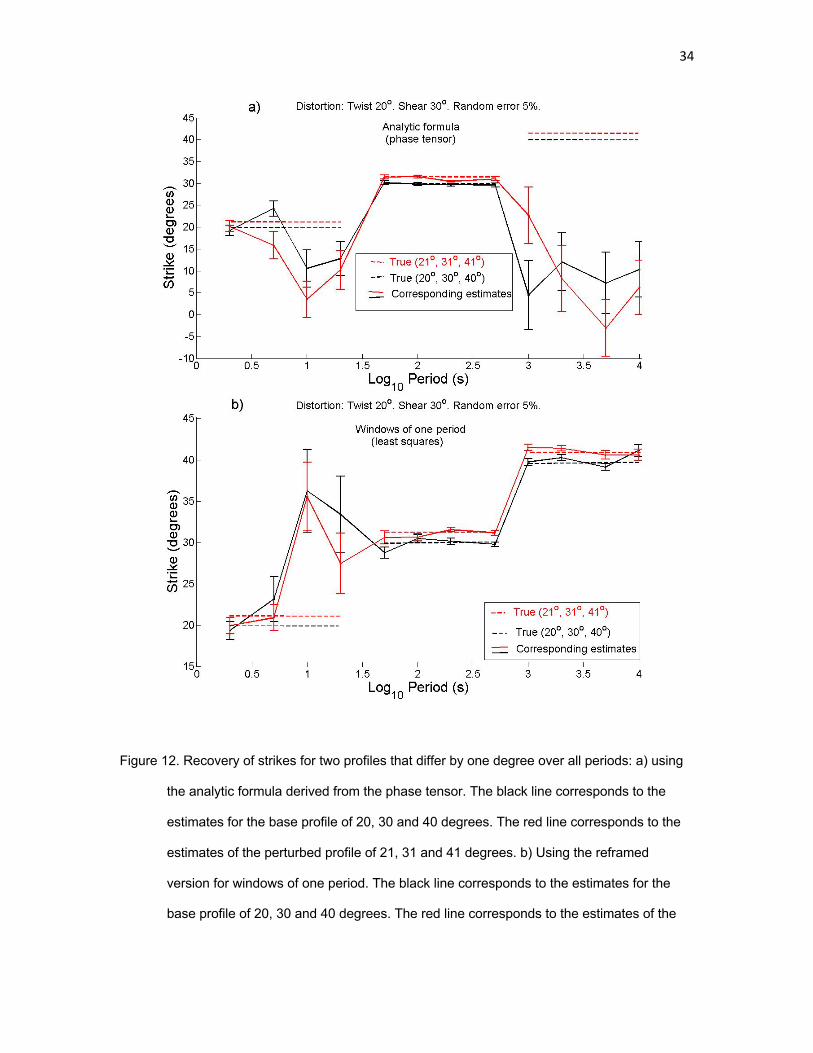
We begin with the analytic formula. It can be observed in Figure 12a that only for

the strike of 30 degrees we have the possibility of hitting the target of one degree

difference. The other two have too large variances and most estimates are way

33

off the desired targets. They not only lack the required precision but also the

required accuracy. As discussed earlier the group of the four central periods is

the better constrained, this corresponds to the strike of 30 degrees. Figure 12b

illustrates the performance of the reframed version using windows of one period.

It can be observed that for the group of 20 degrees the estimations are almost as

bad as those provided by the analytic formula. For the group of 30 degrees the

estimations are comparable for the two approaches. The definite gain is in the

group of 40 degrees where the change of one degree is detected at three out of

four periods. Strictly speaking, and to be fair, the reframed version should be

compared with the analytic formula only when using windows of one period,

which corresponds to the period by period analytic calculations. However, as

discussed earlier, the reframing process allows the use of windows of several

periods. In what follows we only consider only the reframed version.

34

Figure 12. Recovery of strikes for two profiles that differ by one degree over all periods: a) using

the analytic formula derived from the phase tensor. The black line corresponds to the

estimates for the base profile of 20, 30 and 40 degrees. The red line corresponds to the

estimates of the perturbed profile of 21, 31 and 41 degrees. b) Using the reframed

version for windows of one period. The black line corresponds to the estimates for the

base profile of 20, 30 and 40 degrees. The red line corresponds to the estimates of the

35

perturbed profile of 21, 31 and 41 degrees. In both cases the dashed lines represents the

corresponding true values.

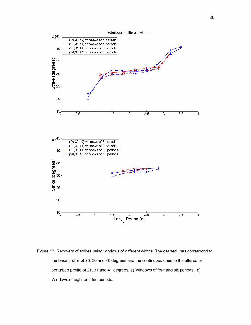
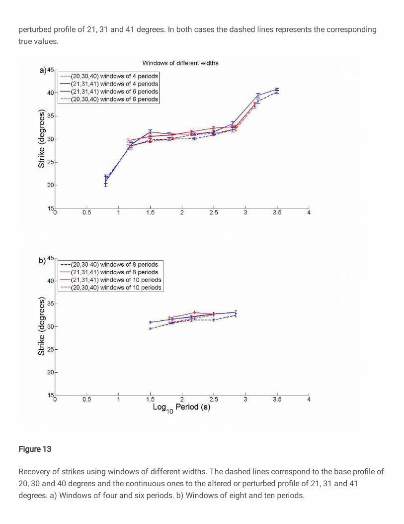
We present results using windows of even number of periods from four to

ten. It is difficult to predict for a non-uniform profile the effect of jumps of strikes

when using windows of several periods because of possible incompatibilities. We

don’t know how the least square criterion can handle very different values at the

same time, and what the effect would be on the variances, which are crucial for

detecting changes. The estimations using windows of four and six periods are

shown in Figure 13a. We will only point out that the estimations improve for most

of the windows except for the first and possibly for the second. Further

improvements can be observed in Figure 13b for windows of eight and ten

periods. Considering these sequence of results, the overall lesson of the exercise

is that we should experiment with windows of different number of periods to

obtain changes that are statistically significant.

36

Figure 13. Recovery of strikes using windows of different widths. The dashed lines correspond to

the base profile of 20, 30 and 40 degrees and the continuous ones to the altered or

perturbed profile of 21, 31 and 41 degrees. a) Windows of four and six periods. b)

Windows of eight and ten periods.

37

APPLICATION TO FIELD DATA

To illustrate the performance of the approach when using field data we

selected a site from a monitoring network installed around the Cerro Prieto

geothermal field, located in northern Baja California, México. Beginning in 2015

with one station the network grew to include up to eighteen by 2018, as new

stations were built at the facilities of CICESE. Electric fields were measured

using 25-m dipoles with a common central Pb-PbCl2 electrode in “L” array, while

magnetic fields used BF-4 type coils. Details about the Pb-PbCl2 electrodes can

be found in Petiau (2000) and Booker and Burd (2006) and about the BF-4 type

coils in the operation manual of the MT-1 system (Electromagnetic Instruments

Inc., 1996). The sampling frequency allowed for a range of periods from about

10-1 to 103 seconds. Only two stations were equipped with induction coils but all

were synchronized for later processing of the time series using remote reference

techniques (Gamble et al., 1979). Specifically, we used the RRRMT8 algorithm

developed by Chave et al. (1987) and Chave and Thomson (1989). More details

about the network are described by Cortés-Arroyo (2018) and Cortés-Arroyo et

al. (2018).

We chose to compare two-week data from 2017 with also two-week data

from 2018 for a station labeled E-4. The comparison follows the last section

where we contrasted synthetic data. First we contrast the performance of the

analytic formula with that obtained using windows of one period. This is

illustrated in Figure 15. In all cases we assumed a 5 % error in the data to

38

compute the errors in the strikes. It can be observed that the estimations using

the formula are very stable for periods between 10 and 100 seconds. In fact it

can be stated that the strike didn’t change from one year to the other in that

range of periods. However, for shorter and longer periods the story is very

different because of the large oscillations in the strike estimates for both years.

Very much the same can be said for the strikes obtained using windows ofone

period except the oscillations are less severe. There is a definite improvement

but certainly not enough to discern a clear change from one year to the other.

Figure 14. Strike estimations using field data from two consecutive years. a) Directly from the

analytic formula. b) Least squares approach using windows of one period. The red lines

correspond to the year 2017 and the blue lines to the year 2018.

39

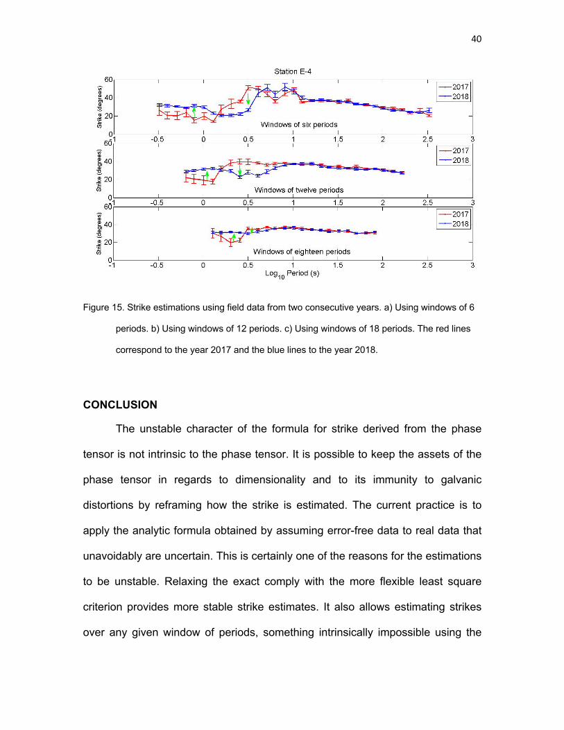
The strikes are a lot smoother when we use windows that include several

periods. There is a total of 36 periods, so choosing windows of 6, 12 and 18

would provide 31, 25 and 19 estimates, respectively. The resulting strikes for

these windows are shown in Figure 16. The estimates for the shortest window

already show a definite trend for the difference between the two years as

illustrated in Figure 16a. This happens for periods shorter than 10 seconds,

which for the area corresponds to depths of penetration of less than 3-4 km. This

would locate the changes within the depth range of the Cerro Prieto geothermal

field, with no appreciable change for the deeper and more regional background.

It is intriguing that the curves cross each other, implying that the strike went a few

degrees to one side for the deeps and to the opposite side for the shallows. This

trend is reproduced for the wider windows of 12 and 18 periods as shown in

Figures 16b and 16c, respectively. However, notice that the negative changes

tend to disappear for the widest window, as indicated by the lowering of the red

curve of 2017 towards the blue of 2018. Notice also the stability and consistency

of the strikes for the longer periods, implying a stable background with a

consistent strike for the two years.

40

Figure 15. Strike estimations using field data from two consecutive years. a) Using windows of 6

periods. b) Using windows of 12 periods. c) Using windows of 18 periods. The red lines

correspond to the year 2017 and the blue lines to the year 2018.

CONCLUSION

The unstable character of the formula for strike derived from the phase

tensor is not intrinsic to the phase tensor. It is possible to keep the assets of the

phase tensor in regards to dimensionality and to its immunity to galvanic

distortions by reframing how the strike is estimated. The current practice is to

apply the analytic formula obtained by assuming error-free data to real data that

unavoidably are uncertain. This is certainly one of the reasons for the estimations

to be unstable. Relaxing the exact comply with the more flexible least square

criterion provides more stable strike estimates. It also allows estimating strikes

over any given window of periods, something intrinsically impossible using the

41

analytic formula. It is worthwhile to remark that the estimation over a given

number of periods is not the average of the individual values of the analytic

formula over those periods. Thus the least squares approach certainly brings

something new to the estimation of strike as opposed to using the analytic

formula. Although in principle the L1 norm is less biased in the presence of

outliers than the L2 norm, we didn’t find significant differences between the two

norms. Regarding uncertainties we didn’t explore beyond the standard deviation

assuming normal distributions. The subject is open for future work using more

elaborated methods as stochastic, Bayesian or Markov chains approaches for

sampling and estimating parameters and their uncertainties. Another extension

would be the implementation of nested algorithms for either imposing continuity

of strikes over period, or getting the optimal combination of window sizes for a

given variance.

DECLARATIONS

Availability of data and materials

The time series of electric and magnetic fields from which Figures 15 and 16 were

obtained are available at CEMIE-Geo’s repository and belong to CICESE. In order to

have access to the data, it would be necessary to make an agreement with CICESE.

Please contact Dr. José Romo (jromo@cicese.mx).

Abbreviations

MT: Magnetotelluric

2D: Two-dimensional

3D: Tree-dimensional

TE: Transverse electric

42

TM: Transverse magnetic

Funding

The work was supported by the Centro Mexicano de Innovación en Energía Geotérmica,

CEMIE-GEO (Project # 207032-2013-04).

Author information

Affiliations

Departamento de Geofísica Aplicada, División de Ciencias de la Tierra, CICESE,

Ensenada, Baja California, México. 22860.

Ana G. Bravo-Osuna, Enrique Gómez-Treviño, Nestor F. Delgadillo-Jauregui and Rocío

F. Arellano-Castro

Federal Institute for Geosciences and Natural Resources (BGR), Berlin, Germany. Olaf

J. Cortés-Arroyo

Contributions

All authors contributed about equally to this work.

All authors read and approved the final manuscript.

Corresponding author

Ana G. Bravo-Osuna

Competing interests

The authors declare that they have no competing interests.

ACKNOWLEDGEMENTS

A.G.B-O, O.J.C-A, N.F.D.J and R.F.A-C acknowledge scholarships from CONACYT for

their graduate work at CICESE. Thanks also to Ricardo Antonio, Enrique Castillo,

Gabriel Echeagaray, Favio Cruz, Miguel Oliver and Jaime Calderón for their support in

the monitoring field trips.

43

REFERENCES

Backus, G., & Gilbert, F. (1968). The resolving power of gross earth

data. Geophysical Journal International, 16(2), 169-205.

Bahr, K. (1988). Interpretation of the magnetotelluric impedance tensor: regional

induction and local telluric distortion. Journal of Geophysics, 62(1), 119-127.

Booker, J., Burd, A. (2006). Second Generation Pb-PbCl2 Electrodes for

Geophysical Applications (Revisited). Poster. 18th International Workshop on

Electromagnetic Induction in the Earth. El Vendrell, España.

Caldwell, T. G., Bibby, H. M., & Brown, C. (2004). The magnetotelluric phase

tensor. Geophysical Journal International, 158(2), 457-469.

Cantwell T (1960) Detection and analysis of low frequency magnetotelluric

signals. PhD Thesis, Massachusetts Institute of Technology.

Chave, A. D., & Jones, A. G. (Eds.). (2012). The magnetotelluric method: Theory

and practice. Cambridge University Press.

Chave, A.D. ,Thomson, D.J., and Ander, M.E. (1987) On the robust estimation of

power spectra, coherences, and transfer functions, J. Geophys. Res., 92: 633-

648.

Chave, A.D., and Thomson, D.J.(1989) Some comments on magnetotelluric

response function estimation, J. Geophys. Res., 94: 14215−14225.

Clarke, J., Gamble, T. D., Goubau, W. M., Koch, R. H., &Miracky, R. (1983).

Remote-reference magnetotellurics: equipment and procedures. Geophysical

Prospecting, 31(1), 149-170.

Constable, S. C., Parker, R. L., & Constable, C. G. (1987). Occam’s inversion: A

practical algorithm for generating smooth models from electromagnetic sounding

data. Geophysics, 52(3), 289-300.

Cortés-Arroyo, O.J. (2018) Monitoreo electromagnético temporal como

herramienta de evaluación en un yacimiento geotérmico. Doctoral thesis.

CICESE, Ensenada, Baja California.

Cortés-Arroyo, O. J., Romo-Jones, J. M., & Gómez-Treviño, E. (2018). Robust

estimation of temporal resistivity variations: Changes from the 2010 Mexicali, Mw

7.2 earthquake and first results of continuous monitoring. Geothermics, 72, 288-

300.

44

Electromagnetic Instruments Inc (1996) MT-1 magnetotelluric system operation

manual.

Gamble, T.D., Goubau, W.M., and Clarke, J. (1979) Magnetotellurics with a

remote magnetic reference. Geophysics,44 (1): 53–68.

Groom, R. W., & Bailey, R. C. (1989). Decomposition of magnetotelluric

impedance tensors in the presence of local three-dimensional galvanic

distortion. Journal of Geophysical Research: Solid Earth, 94(B2), 1913-1925.

Jones, A. (2012) Distortion of magnetotelluric data: its identification and removal.

The Magnetotelluric Method. Theory and Practice: 219-302.

McNeice, G. W., & Jones, A. G. (2001). Multisite, multifrequency tensor

decomposition of magnetotelluric data. Geophysics, 66(1), 158-173.

Muñíz, Y., Gómez-Treviño, E., Esparza, F. J., & Cuellar, M. (2017). Stable 2D

magnetotelluric strikes and impedances via the phase tensor and the quadratic

equation. Geophysics, 82(4), E169-E186.

Peacock, J. R., Thiel, S., Heinson, G. S., & Reid, P. (2013). Time-lapse

magnetotelluric monitoring of an enhanced geothermal

system. Geophysics, 78(3), B121-B130.

Peacock, J.R., Thiel, S., Reid, P., and Heinson, G. (2012) Magnetotelluric

monitoring of a fluid injection: Example from an enhanced geothermal system.

Geophysical Research Letters,39, L18403.

Petiau, G. (2000) Second Generation of Lead-lead Chloride Electrodes for Geophysical Applications. Pure and Applied Geophysics 157, 357 -382. Simpson, F., & Bahr, K. (2005). Practical magnetotellurics. Cambridge University

Press.

Swift, C. M. (1967). A magnetotelluric investigation of an electrical conductivity

anomaly in the southwestern United States (Doctoral dissertation, Massachusetts

Institute of Technology).

Varentsov, I.M., 1998. 2D synthetic data sets COPROD-2S to study MT inversion

techniques, Presented at the 14th Workshop on Electromagnetic Induction in the

Earth, Sinaia, Romania, Available at: http://mtnet.dias.ie.

Vozoff, K. (1972). The magnetotelluric method in the exploration of sedimentary

basins. Geophysics, 37(1), 98-141.

45

Figures

Figure 1

The elements of the impedance tensor correspond to site 15 of the COPROD2S1 dataset. The originalimpedances were distorted and random noise added as indicated. a) Real parts. b) Imaginary parts. Thevalues were computed as the mean of 30 realizations per period with their corresponding standard

deviations. The continuous lines join the error-free values which in most cases are practically identical tothe mean values.

Figure 2

a) Diagonal elements of the phase tensor derived from the impedance tensor shown in Figure 1. Thecolor code is Φ_11 green and Φ_22 yellow. The black continuous line corresponds to error-free values. b)

The corresponding off-diagonal elements. The color code is. Φ_12 green and Φ_21 yellow. The blackdashed line corresponds to error-free values.

Figure 3

a) Combination of the phase tensor elements that make up the ratio in the formula for the angle α. Thecolor code is Φ_11 - Φ_22 green and Φ_12 + Φ_21 yellow. The black continuous line corresponds to error-

free values. b) Corresponding combination for the angle β. The color code is Φ_11+ Φ_22 green and Φ_12- Φ_21 yellow. The black dashed line corresponds to error-free values.

Figure 4

a) The ratios that make up the formulae for the angles α and β. The color code is green for the angle αand yellow for the angle β. The black continuous line corresponds to error- free values. b) The �nal resultsfor the strike θ=α-β. The red line corresponds to estimates assuming 1% error and using 30 realizations.

The black line corresponds to 1% error and 1000 realizations. The dashed blue line corresponds to 0.01%error and 30 realizations.

Figure 5

The analysis of the formula for strike indicates that it is biased with respect to random noise: a) theindividual strikes for each realization are plotted for two levels of error. The green lines correspond to 1%error and 1000 realizations. The yellow lines correspond to 5% error and 1000 realizations. The data were

distorted assuming twist= 20° and shear =30°. The dashed line represents the true strike as computedwith 0.01 % error. b) The black line represents the estimates of strikes using 5 % error and 30 realizations.The red line represents the estimates using 5 % error and 1,000 realizations The analysis of the formulafor strike indicates that it is biased with respect to random noise: a) the individual strikes for eachrealization are plotted for two levels of error. The green lines correspond to 1% error and 1000realizations. The yellow lines correspond to 5% error and 1000 realizations. The data were distortedassuming twist= 20° and shear =30°. The dashed line represents the true strike as computed with 0.01 %error. b) The black line represents the estimates of strikes using 5 % error and 30 realizations. The red linerepresents the estimates using 5 % error and 1,000 realizations

Figure 6

Determination of strike angles using the phase tensor and Swift’s approach: a) with no galvanicdistortions. The black dashed line represents the true strike. The black continuous line represents theestimates using Swift’s least squares approach applied to the elements of the impedance tensor. The redline corresponds to the estimates using the analytic formula derived from the phase tensor. b) Withgalvanic distortions. The black dashed line represents the true strike. The black continuous line

represents the estimates using Swift’s least squares approach applied to the elements of the impedancetensor. The red line corresponds to the estimates using the analytic formula derived from the phasetensor.

Figure 7

The black continuous line represents the estimates using the least squares approach applied to theelements of the phase tensor and windows of one period. The red line corresponds to the estimates usingthe analytic formula derived from the phase tensor. The dashed line represents the true value.

Figure 8

The red line corresponds to estimates of strike using the analytic formula. The black line represent theestimates using the least squares approach assuming windows of four periods. The horizontal barsrepresent the width of the windows. These graphs illustrate that the estimates using windows of fourperiods are not averages of those provided by the analytic formula, as clearly illustrated by the �rst andlast four periods. The windows of four periods were chosen on purpose to show this property.

Figure 9

Comparison between theL_1 andL_2 norms using windows of three periods. The improvement of usingthe former over the latter is very marginal. We had to increase the random errors to 10% to obtain anoticeable difference. The red line corresponds to the L_2 norm and the black line to the L_1 norm.

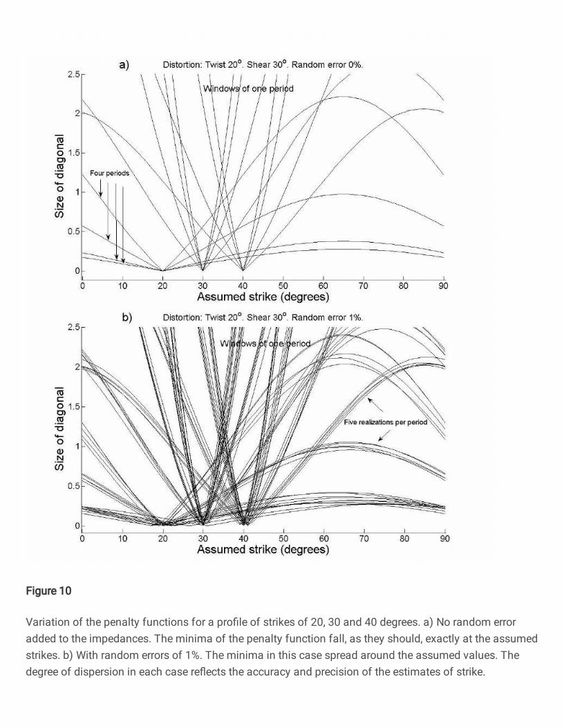
Figure 10

Variation of the penalty functions for a pro�le of strikes of 20, 30 and 40 degrees. a) No random erroradded to the impedances. The minima of the penalty function fall, as they should, exactly at the assumedstrikes. b) With random errors of 1%. The minima in this case spread around the assumed values. Thedegree of dispersion in each case re�ects the accuracy and precision of the estimates of strike.

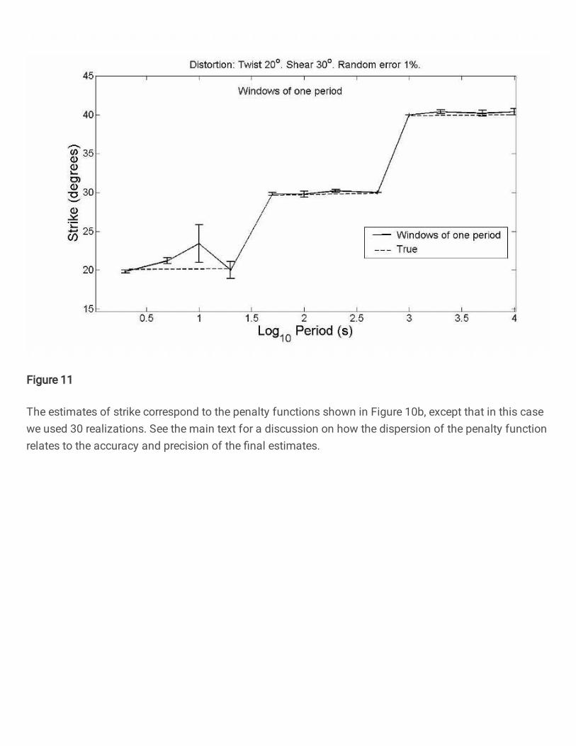
Figure 11

The estimates of strike correspond to the penalty functions shown in Figure 10b, except that in this casewe used 30 realizations. See the main text for a discussion on how the dispersion of the penalty functionrelates to the accuracy and precision of the �nal estimates.

Figure 12

Recovery of strikes for two pro�les that differ by one degree over all periods: a) using the analytic formuladerived from the phase tensor. The black line corresponds to the estimates for the base pro�le of 20, 30and 40 degrees. The red line corresponds to the estimates of the perturbed pro�le of 21, 31 and 41degrees. b) Using the reframed version for windows of one period. The black line corresponds to theestimates for the base pro�le of 20, 30 and 40 degrees. The red line corresponds to the estimates of the

perturbed pro�le of 21, 31 and 41 degrees. In both cases the dashed lines represents the correspondingtrue values.

Figure 13

Recovery of strikes using windows of different widths. The dashed lines correspond to the base pro�le of20, 30 and 40 degrees and the continuous ones to the altered or perturbed pro�le of 21, 31 and 41degrees. a) Windows of four and six periods. b) Windows of eight and ten periods.

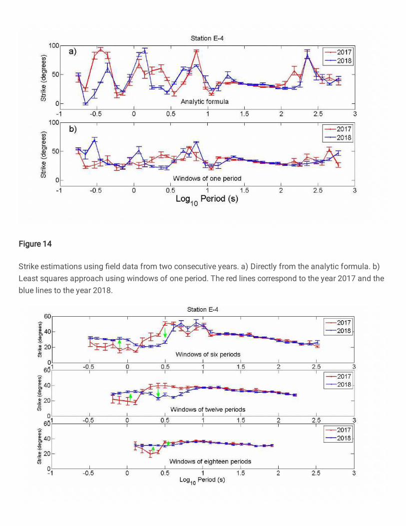
Figure 14

Strike estimations using �eld data from two consecutive years. a) Directly from the analytic formula. b)Least squares approach using windows of one period. The red lines correspond to the year 2017 and theblue lines to the year 2018.

Figure 15

Strike estimations using �eld data from two consecutive years. a) Using windows of 6 periods. b) Usingwindows of 12 periods. c) Using windows of 18 periods. The red lines correspond to the year 2017 andthe blue lines to the year 2018.

Supplementary Files

This is a list of supplementary �les associated with this preprint. Click to download.

GraphRev.png

APPENDIX.docx