Reduced-order models of linearized channel flow using balanced truncation

Clarence W. Rowley and Milos Ilak

Abstract— Fluid systems often exhibit inherently low-dimensional behavior, even though the governing equations arecomplex and high-dimensional. At this time, full 3D discretiza-tions of the Navier-Stokes equations are too computationallyintensive to be used for control synthesis, so low-order modelsof the flow physics are desirable. This paper compares twodifferent model-reduction procedures for the linearized flow in aplane channel: the method of Proper Orthogonal Decompositionand Galerkin projection, popular in the fluid mechanics com-munity; and balanced truncation, a common method for modelreduction of linear systems. Standard methods of computingbalancing transformations are computationally intractable forsystems of this size, so we use a numerical approximationof balanced truncation using empirical Gramians computedfrom simulations of the linearized and adjoint systems. For thechannel flow considered here, the subspaces spanned by PODmodes and balancing modes are very close, but reduced-ordermodels from approximate balanced truncation perform muchbetter than the standard POD models, for the same order oftruncation.

I. INTRODUCTION

A better understanding of the mechanisms leading totransition from laminar to turbulent flow, and the potentialfor actuators to affect these mechanisms, may lead to dragreduction and substantial fuel savings for aircraft and otherapplications. This paper discusses low-dimensional modelsfor a transitional flow, and compares two different tech-niques, focusing on the effects of actuation on the flow.

The incompressible flow in a plane channel is considered,and in particular this study focuses on the linearized equa-tions, as in several previous studies [1], [2], [3], [4], [5]. Webegin with the linearized Navier-Stokes equations and obtainreduced-order models using two separate approaches: projec-tion of the governing equations onto empirical basis func-tions found from Proper Orthogonal Decomposition (POD)of data from simulations; and balanced truncation. Whilethe POD/Galerkin method is computationally tractable evenfor very large systems, and has been used on many fluidsproblems, including boundary layers [6], cavity flows [7], [8],cylinder wakes [9], airfoils [10], and many others, balancedtruncation has been used for fluids problems by only a fewresearchers [3], [2], and even then, in only one spatial dimen-sion, because the computations rapidly become intractable asthe number of states increases. In a typical fluids problem,the number of states is on the order of 105 or more, andsince computing balancing transformations involves solving

This work was supported by the National Science Foundation, awardCMS-0347239

C.W. Rowley and M. Ilak are with the Department of Mechanical andAerospace Engineering, Princeton University, Princeton, NJ 08544, USAcwrowley@princeton.edu, milak@princeton.edu

n×n Lyapunov equations (where n > 105 is the number ofstates) as well as correspondingly large eigenvalue problems,traditional approaches to balanced truncations may not befeasible. Recently, snapshot-based methods for computingbalanced truncations have been suggested, both to extendthe concepts to nonlinear systems [11], [12] and to largelinear systems [13]. In the present paper, we apply thesemethods to models of plane channel flow, and compare theresulting models to POD/Galerkin models. In §II we give abrief overview of these model reduction methods; in §III wedescribe the channel flow studied; and in §IV we comparethe low-order models obtained by the various methods.

II. MODEL REDUCTION METHODS

Here, we review the two model reduction methods wewill compare: Galerkin projection onto basis functions de-termined by Proper Orthogonal Decomposition (POD) of aparticular dataset [14], [15]; and balanced truncation, usingempirical Gramians built from snapshots from simulationsof impulse responses [11], [12], [13].

A. POD and Galerkin projection

The idea of Galerkin projection is, given dynamics

x = f(x), x(t) ∈ X ,

where X is a high-dimensional Hilbert space, to project ontoa low-dimensional subspace S ⊂ X , i.e., obtaining a reducedorder model for a variable r ∈ S as

r = PSf(r),

where PS : X → S is the orthogonal projection. One wayof choosing this subspace S is to gather a set of data xj ∈X | j = 1, . . . m representative of typical behavior of thesystem, and to determine the subspace of a fixed dimensionthat optimally spans this dataset:

S = arg minS

m∑j=1

‖xj − PSxj‖2. (1)

Proper Orthogonal Decomposition determines an orthogonalbasis for such a subspace, which may be computed by findingthe left singular vectors of the data matrix, whose columnsare the snapshots xj .

Advantages of the POD/Galerkin method are that it iscomputationally tractable even for very large datasets, forinstance, even when the dimension of X is on the order ofmillions, as is often the case for typical fluids simulations.However, disadvantages are that the subspace determinedby (1) truncates the lowest-energy modes, and low-energy

modes may be important for the dynamics. For linearsystems, another interpretation is that the POD modes ofdata arising from the input-state impulse response are themost controllable modes of the linear system (eigenvectorscorresponding to largest eigenvalues of the controllabilityGramian) [13], so projecting onto these may neglect im-portant modes that may be weakly controllable but stronglyobservable. Another disadvantage is that the method dependson the choice of inner product, and different inner productscan drastically change the behavior of the models [13],and even the stability type of equilibria [7]. Ideally, onecould imagine optimizing over not just the choice of thesubspace, but also the choice of inner product. The methoddescribed in the next section achieves this goal at leastpartially: while not optimal, balanced truncation essentiallydoes select both the subspace for projection and the innerproduct for projection, not through an optimization, butthrough a heuristic procedure that typically performs verywell, and has provable error bounds.

B. Snapshot-based balanced truncation

Balanced truncation is typically used for model reductionof stable linear input-output systems of the form

x = Ax + Bu

y = Cx(2)

where x(t) ∈ X is the state, u(t) ∈ U is the input, andy(t) ∈ Y is the output, and X , U , and Y are Hilbert spaces.If the system is both controllable and observable, one candetermine a coordinate system in which the controllabilityand observability Gramians, defined respectively by

Wc =∫ ∞

0

eAtBB∗eA∗t dt, Wo =∫ ∞

0

eA∗tC∗CeAt dt,

(3)are equal and diagonal (equal to the matrix of Hankelsingular values). One then truncates the states that are leastcontrollable and observable, corresponding to the smallestHankel singular values [16], [17]. This procedure, while notactually optimal in any known sense, has H∞ error boundsthat are typically close to the best attainable by any reducedorder model: recall that the error between a full model G(s)and any reduced order model Gr(s) with state dimension ris bounded by

‖G−Gr‖∞ ≥ σr+1,

where σj is the j-th Hankel singular value (in decreasingorder). Extensions are also available for unstable [18], [19]and nonlinear systems [11], [20].

Here, we are interested in the case where the dimensionof X is very large, on the order of millions, so directcomputation of the full Gramians is not possible. In ad-dition, the output space Y may be very large as well:for instance, we may be interested in capturing an entirefluid flow field accurately, so that the output is the entirestate (though possibly with a different inner product). Inorder to compute the balancing transformation in this case,we construct empirical Gramians, as in [11], and compute

the balancing transformation using the method of snapshotsdescribed in [13], in which one uses a single SVD of a datamatrix formed by inner products of snapshots from forwardand adjoint simulations, as described below.

1) Empirical Gramians: Here, we will assume that thenumber of inputs u is small. We first perform simulationsof the system (2), with x(0) = 0, and implusive inputs oneach component of u. After [11], the empirical controllabilityGramian may be computed by assembling the snapshotsfrom these simulations (solutions x(tj) at different timestj , j = 1, . . . ,m) as columns of a matrix X : Rm →X , appropriately weighted by quadrature coefficients sothat Wc = XX∗ approximates the integral (3). One maycompute the empirical observability Gramian analogously,by computing solutions to the adjoint system

z = A∗z + C∗v, v ∈ Y (4)

forward in time, with z(0) = 0 and impulses on eachcomponent of v. Here C∗ : Y → X is the adjoint of C : X →Y , which of course depends on the inner products in both Xand Y , so care must be taken if nonstandard inner productsare used (as they will be in §III). From these simulations, oneobtains l snapshots zj which are appropriately weighted andassembled as columns of a data matrix Y : Rl → X , so thatthe observability Gramian in (3) is approximated by Y Y ∗.

Note that if the number of outputs is large, the computationof the adjoint snapshots may not be tractable, since onesimulation is needed for each component of the output.Below, we will consider the output y = x, as we wishour model to reproduce the full flow information, so thenumber of outputs is indeed large, and we require an alternateapproach. In particular, we first project the output onto alow-dimensional subspace, i.e., taking y = PrCx, where Pr

is an orthogonal projection onto an r-dimensional subspaceof Y . Conveniently, the projection Pr that minimizes the 2-norm of the difference between the original transfer functionand the output-projected transfer function is given simply byPOD of the set of impulse responses, which has already beencomputed in the previous step [13]. Writing this projectionas Pr = ΦrΦ∗r , where columns of Φr : Rr → Y are PODmodes, one needs only to compute r impulse responses ofthe system

z = A∗z + C∗Φrw, w ∈ Rr. (5)

2) Balancing transformation: Once the primal and adjointsnapshots are computed, as described in [13], the balancingtransformation that diagonalizes the empirical Gramians maybe found by an SVD of the matrix Y ∗X : Rm → Rl, whosedimensions are the number of primal snapshots × the numberof adjoint snapshots, which is typically manageable (e.g.,< 104). Forming the SVD

Y ∗X = UΣV ∗, (6)

one easily shows Σ ∈ Rp×p is the diagonal matrix of nonzeroHankel singular values, and U ∈ Rl×p and V ∈ Rm×p

x

y

zU(y)

Fig. 1. Flow geometry for plane channel flow.

satisfy U∗U = V ∗V = Ip. The balancing transformationis then found by computing matrices

T = XV Σ−1/2, S = Σ−1/2U∗Y ∗ (7)

which satisfy ST = Ip. If p = n (i.e., if the system iscontrollable and observable, and enough snapshots have beentaken), then T = S−1 is the transformation that diagonalizesthe Gramians. If p < n, as will be the case here, then asshown in [13], T block diagonalizes the empirical Gramians,extracting the first p Hankel singular values.

Knowing both S and T , one may obtain balanced trunca-tions directly, without literally transforming the entire state tonew coordinates (which would be computationally intractablefor systems of this order) and subsequently truncating. If qis the desired order of the reduced-order model, one lets T1

denote the first q columns of T , and S1 the first q rows ofS, and then the reduced-order model is given by

z = S1AT1z + S1B

y = CT1z

Note, however, that this is not equivalent to orthogonalprojection onto the first q columns of T , since these columnsare not orthogonal with respect to the standard inner product.(Instead, the columns of T and the rows of S form a bi-orthogonal set, as discussed in [13].)

III. PLANE CHANNEL FLOW

We consider the flow between two parallel plates, as indi-cated in Fig. 1. The domain is periodic in the streamwise xand spanwise z directions, and we linearize about a laminarbase flow. (Here, x, y, and z denote coordinates in physicalspace, not to be confused with the state, output, and adjointvariables from the previous section.) Nondimensionalizingby the channel half-height δ and the centerline velocity Ucl,the base flow has the form U(y) = 1− y2.

A. Linearized equations

For this geometry, the linearized equations may be conve-niently written in terms of the wall-normal velocity v and thewall-normal vorticity η [1]. The other variables (e.g., stream-wise and spanwise velocities u and w) may then be computedusing the continuity equation ∂xu+∂yv+∂zw = 0. In thesecoordinates, the linearized (nondimensional) equations havethe form

∂

∂t

[−∆ 00 I

] [vη

]=

[LOS 0−U ′∂z LSQ

] [vη

](8)

where ∆ = ∂2x + ∂2

y + ∂2z is the Laplacian, and

LOS = U∂x∆− U ′′∂x −1R

∆2

LSQ = −U∂x +1R

∆

are the Orr-Sommerfeld and Squire operators, respectively.Here, R = Uclδ/ν is the Reynolds number, where ν is thekinematic viscosity. It has been shown numerically that theabove linearized system is stable up to R ≈ 5772, thoughsevere non-normality exists, and large transient response isobserved [21], [1], [5].

B. Inner product and adjoint equations

To determine the corresponding adjoint equations, one firstneeds to define an inner product on the vector space X offlow variables (v, η). It will be convenient to define the innerproduct

〈(v1, η1), (v2, η2)〉 =∫

Ω

(−v1∆v2 + η1η2) dx dy dz,

where Ω denotes the fluid volume. Note that, letting M :X → X denote the operator on the left hand side of (8), thisis just the L2 inner product of (v1, η1) with M(v2, η2).

With this definition of the inner product, the adjointequations are easily found by integration by parts:

∂

∂t

[−∆ 00 I

] [vη

]=

[L∗OS U ′∂z

0 L∗SQ

] [vη

](9)

where

L∗OS = −U∂x∆− 2U ′∂x∂y −1R

∆2

L∗SQ = U∂x +1R

∆.

C. Numerical method

Both the linearized (8) and adjoint (9) equations aresolved numerically, using Fourier modes in the x and zdirections and Chebyshev polynomials in the wall-normal(y) direction, using a method similar to that in [22]. Twodifferent simulations are considered here: first, for validationpurposes, streamwise-constant perturbations are considered,at a grid resolution that is small enough that exact balancedtruncation may be computed using standard routines inMatlab (16×17 gridpoints, state dimension n = 480). Next,full 3D perturbations are considered at a grid resolution forwhich exact balanced truncation is intractable (16× 17× 16grid, n = 7680). For both cases, the R = 100, witha domain [0, 2π] in the x and z directions. To computethe POD and balancing modes, both simulations use 1000snapshots equally spaced in the interval t ∈ [0, 200], andthe timestep for the simulations is 0.002 for both linearizedand adjoint simulations. Though the grid is coarse, thesimulations are fully resolved at this Reynolds number, withthe first gridpoint from the wall at y+ = 0.27.

0 2 4 6 8 1010!8

10!6

10!4

10!2

100

102

r (order of reduced model)

‖Gr −G‖∞‖G‖∞

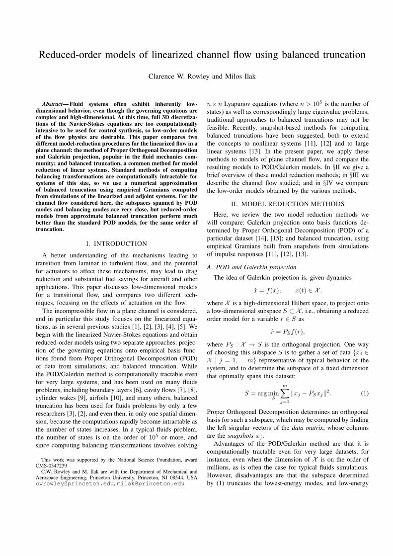
Fig. 2. Error norms of reduced-order models, for streamwise-constant per-turbations: POD/Galerkin (4), full balanced truncation (×), approximate,snapshot-based balanced truncation, with 5-mode () and 10-mode ()output projections; and lower bound for any reduced-order model (—).

IV. RESULTS

A. Streamwise-constant perturbations

Figure 2 shows H∞ norms for the error between the fullorder model, whose transfer function is denoted G(s), andreduced-order models of state dimension r, whose transferfunction is denoted Gr(s). Here, the system is small enough(n = 480) that exact balanced truncation may be computedusing standard routines, and the error from the snapshot-based approximate balanced truncation is almost identical tothat from the full balanced truncation. For most values of r,the errors from balanced truncation, either exact or snapshot-based, are smaller than the error from the POD/Galerkinmodel, and are close to the lower bound for any reduced-order model (obtained from the magnitude of the first trun-cated Hankel singular value [17]). For further results onthe streamwise-constant case, including plots of the modesthemselves, see [13] (in this reference, a slightly differentforcing term was used, but results are qualitatively the same).

B. Three-dimensional perturbations

Full three-dimensional perturbations were introduced us-ing a localized body force in a small region in the center ofthe domain. Sample velocity fields at two separate times (t =9 and t = 30) are shown in Fig. 3, which illustrate how thelocalized perturbation becomes stretched in the streamwisedirection, and eventually resembles the streamwise-constantperturbations considered earlier.

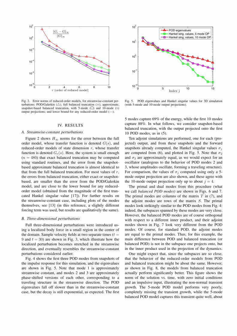
Fig. 4 shows the first three POD modes from snapshots ofthe impulse response for this simulation, and the eigenvaluesare shown in Fig. 5. Note that mode 1 is approximatelystreamwise constant, and modes 2 and 3 are approximatelyphase-shifted versions of each other, corresponding to atraveling structure in the streamwise direction. The PODeigenvalues fall off slower than in the streamwise-constantcase, but the decay is still exponential, as expected. The first

0 5 10 1510!2

10!1

100

101

102

POD eigenvaluesHankel sing. values, 5 mode OPHankel sing. values, 10 mode OP

Index j

Fig. 5. POD eigenvalues and Hankel singular values for 3D simulation(with 5-mode and 10-mode output projections).

5 modes capture 69% of the energy, while the first 10 modescapture 88%. In what follows, we consider snapshot-basedbalanced truncation, with the output projected onto the first10 POD modes, as in (5).

Ten adjoint simulations are performed, one for each (pro-jected) output, and from these snapshots and the forwardsnapshots already computed, the Hankel singular values σj

are computed from (6), and plotted in Fig. 5. Note that σ2

and σ3 are approximately equal, as we would expect for anoscillator (analogous to the behavior of POD modes 2 and3, whose amplitudes oscillate, forming a traveling structure).For comparison, the values of σj computed using only a 5-mode output projection are also shown, and these agree withthe 10-mode output projection only up to about j = 4.

The primal and dual modes from this procedure (whatwe call balanced POD modes) are shown in Figs. 6 and 7.The primal modes are columns of the matrix T in (7), andthe adjoint modes are rows of the matrix S. The primalmodes look strikingly similar to the POD modes from Fig. 4:indeed, the subspaces spanned by these modes are very close.However, the balanced POD modes are of course orthogonalwith respect to a different inner product, and their adjointmodes shown in Fig. 7 look very different from the PODmodes. Of course, for standard POD, the adjoint modesare equal to the primal modes. Thus, for this example, themain difference between POD and balanced truncation (orbalanced POD) is not in the subspace one projects onto, butin the inner product used in the projection of the dynamics.

One might expect that, since the subspaces are so close,that the behavior of the reduced-order models from PODand balanced truncation might be about the same. However,as shown in Fig. 8, the models from balanced truncationactually perform significantly better. This figure shows thenorm of the solution vs. time, with zero initial conditionsand an impulsive input, illustrating the non-normal transientgrowth. The 5-mode POD model performs very poorly,completely missing the transient growth, while the 5-modebalanced POD model captures this transient quite well, about

Fig. 3. Contours and level sets of wall-normal vorticity η from the response to an impulsive body force in a small region in the center of the domain, attime t = 9 (left) and t = 30 (right), showing the evolution of streamwise structures. Flow is left to right, and walls are at the top and bottom.

Fig. 4. First three POD modes from impulse response of 3D simulation, showing contours and level sets of wall-normal velocity v (top) and vorticity η(bottom).

Fig. 6. First three primal modes from balanced POD, showing wall-normal velocity v (top) and vorticity η (bottom).

Fig. 7. First three adjoint modes from balanced POD, showing wall-normal velocity v (top) and vorticity η (bottom).

0 20 40 60 80 1000

0.1

0.2

0.3

0.4

0.5

0.6

0.7Full simulationBalanced POD, 5 modesStandard POD, 5 modesBalanced POD, 10 modesStandard POD, 10 modes

Time t

L2

norm

ofso

luti

on

Fig. 8. Norm of impulse response for full simulation, compared withreduced-order models from POD and balanced POD. Note that the 5-modebalanced POD model captures the non-normal transient growth about aswell as the 10-mode model using standard POD, while the 5-mode standardPOD model completely misses the transient growth.

as well as the 10-mode POD model. The curve for 10-mode balanced POD is almost identical to that of the fullsimulation.

REFERENCES

[1] P. J. Schmid and D. S. Henningson, Stability and Transition in ShearFlows, ser. Applied Mathematical Sciences. Springer-Verlag, 2001,vol. 142.

[2] B. F. Farrell and P. J. Ioannou, “Accurate low-dimensional approxima-tion of the linear dynamics of fluid flow,” J. Atmospheric Sci., vol. 58,pp. 2771–2789, 2001.

[3] K. H. Lee, L. Cortelezzi, J. Kim, and J. Speyer, “Application ofreduced-order controller to turbulent flows for drag reduction,” Phys.Fluids, vol. 13, no. 5, pp. 1321–1330, 2001.

[4] B. Bamieh and M. Daleh, “Energy amplification in channel flows withstochastic excitation,” Phys. Fluids, vol. 13, no. 11, pp. 3258–3269,Nov. 2001.

[5] M. R. Jovanovic and B. Bamieh, “Input-output analysis of the lin-earized Navier-Stokes equations in channel flows,” J. Fluid Mech.,no. Submitted, 2003.

[6] N. Aubry, P. Holmes, J. L. Lumley, and E. Stone, “The dynamics ofcoherent structures in the wall region of a turbulent boundary layer,”J. Fluid Mech., vol. 192, pp. 115–173, 1988.

[7] C. W. Rowley, T. Colonius, and R. M. Murray, “Model reduction forcompressible flow using POD and Galerkin projection,” Phys. D, vol.189, no. 1–2, pp. 115–129, Feb. 2004.

[8] N. E. Murray and L. S. Ukeiley, “Estimation of the flowfield fromsurface pressure measurements in an open cavity,” AIAA J., vol. 41,pp. 969–972, 2003.

[9] G. Tadmor, B. Noack, A. Dillmann, J. Gerhard, M. Pastoor, R. King,and M. Morzynski, “Control, observation and energy regulation ofwake flow instabilities,” in 42nd IEEE Conference on Decision andControl, Maui, HI, U.S.A., Dec. 2003, pp. 2334–2339, weM10-4.

[10] J. A. Taylor and M. N. Glauser, “Towards practical flow sensing andcontrol via pod and lse based low-dimensional tools,” J. Fluids Eng.,vol. 126, no. 3, pp. 337–345, May 2004.

[11] S. Lall, J. E. Marsden, and S. Glavaski, “Empirical model reductionof controlled nonlinear systems,” in Proceedings of the IFAC WorldCongress, vol. F, July 1999, pp. 473–478.

[12] ——, “A subspace approach to balanced truncation for model reduc-tion of nonlinear control systems,” Int. J. Robust Nonlinear Control,vol. 12, pp. 519–535, 2002.

[13] C. W. Rowley, “Model reduction for fluids using balanced properorthogonal decomposition,” Int. J. Bifurcation Chaos, vol. 15, no. 3,pp. 997–1013, Mar. 2005.

[14] L. Sirovich, “Turbulence and the dynamics of coherent structures, partsI–III,” Q. Appl. Math., vol. XLV, no. 3, pp. 561–590, Oct. 1987.

[15] P. Holmes, J. L. Lumley, and G. Berkooz, Turbulence, CoherentStructures, Dynamical Systems and Symmetry. Cambridge, UK:Cambridge University Press, 1996.

[16] B. C. Moore, “Principal component analysis in linear systems: Con-trollability, observability, and model reduction,” IEEE Trans. Automat.Contr., vol. 26, no. 1, pp. 17–32, Feb. 1981.

[17] G. E. Dullerud and F. Paganini, A Course in Robust Control Theory:A Convex Approach, ser. Texts in Applied Mathematics. Springer-Verlag, 1999, vol. 36.

[18] E. A. Jonckheere and L. M. Silverman, “A new set of invariants forlinear systems—application to reduced order compensator design,”IEEE Trans. Automat. Contr., vol. 28, no. 10, pp. 953–964, 1983.

[19] K. Zhou, G. Salomon, and E. Wu, “Balanced realization and modelreduction for unstable systems,” Int. J. Robust and Nonlin. Contr.,vol. 9, no. 3, pp. 183–198, Mar. 1999.

[20] J. M. A. Scherpen, “Balancing for nonlinear systems,” Sys. ControlLett., vol. 21, no. 2, pp. 143–153, 1993.

[21] L. N. Trefethen, A. E. Trefethen, S. C. Reddy, and T. A. Driscoll,“Hydrodynamic stability without eigenvalues,” Science, vol. 261, pp.578–584, July 1993.

[22] J. Kim, P. Moin, and R. Moser, “Turbulence statistics in fully-developed channel flow at low Reynolds number,” J. Fluid Mech.,vol. 177, pp. 133–166, Apr. 1987.