1

Recursive Segmentation and Recognition Templatesfor Image Parsing

Long (Leo) Zhu1, Yuanhao Chen2, Yuan Lin3, Chenxi Lin4, Alan Yuille2,5

1CSAIL, MIT. leozhu@csail.mit.edu2Department of Statistics, UCLA. yuille@stat.ucla.edu

3Shanghai Jiaotong University. loirey@sjtu.edu.cn4Alibaba Group R&D. chenxi.lin@alibaba-inc.com

5 Department of Brain and Cognitive Engineering, Korea University

Abstract—In this paper, we propose a HierarchicalImage Model (HIM) which parses images to performsegmentation and object recognition. The HIM representsthe image recursively by segmentation and recognitiontemplates at multiple levels of the hierarchy. This hasadvantages for representation, inference, and learning.Firstly, the HIM has a coarse-to-fine representation whichis capable of capturing long-range dependency and ex-ploiting different levels of contextual information (simi-lar to how natural language models represent sentencestructure in terms of hierarchical representations such asverb and noun phrases). Secondly, the structure of theHIM allows us to design a rapid inference algorithm,based on dynamic programming, which yields the firstpolynomial time algorithm for image labeling. Thirdly, welearn the HIM efficiently using machine learning methodsfrom a labeled dataset. We demonstrate that the HIM iscomparable with the state-of-the-art methods by evaluationon the challenging public MSRC and PASCAL VOC 2007image datasets.

I. INTRODUCTION

Language and image understanding are two majortasks in artificial intelligence. Natural language re-searchers have formalized this task in terms of pars-ing an input signal into a hierarchical representation.They have made great progress in both representa-tion and inference (i.e. parsing). Firstly, they havedeveloped probabilistic grammars (e.g. stochasticcontext free grammar (SCFG) [1] and beyond [2])which are capable of representing complex syntacticand semantic language phenomena. For example,language contains elementary constituents, such asnouns and verbs, that can be recursively composedinto a hierarchy (e.g. noun phrase or verb phrase)of increasing complexity. Secondly, they have ex-ploited the one-dimensional structure of language to

obtain efficient polynomial-time parsing algorithms(e.g. the inside-outside algorithm [3]).

By contrast, the nature of images makes it muchharder to design efficient image parsers which arecapable of simultaneously performing segmentation(parsing an image into regions) and recognition(labeling the regions). Firstly, it is unclear whathierarchical representations should be used to modelimages because there are no direct analogies tothe syntactic categories and phrase structures thatoccur in language. Secondly, the inference problemis formidable due to the well-known complexityand ambiguity of segmentation and recognition. Inmost languages the boundaries between differentwords are well-defined (Chinese is an exception)but, by contrast, the segmentation boundaries be-tween different image regions are usually highlyunclear. Exploring all the different image partitionsrisks a combinatorial explosions because of the two-dimensional nature of images (dynamic program-ming methods can be used for one-dimensionaldata such as language). Overall it has been hardto adapt methods from natural language parsingand apply them to vision despite the high-levelconceptual similarities (except for restricted andhighly structured problems such as text [4]).

We argue that to make progress at image parsingrequires making trade-offs between the complexityof the representation and the complexity of thecomputation (for inference and learning). Our workbuilds on three themes in the recent literature.Firstly, the use of stochastic grammars to representimages and objects [5], [6], [7], [8]. This styleof research uses generative models for images andpays less attention to the complexity of compu-

2

tation. Inference is usually performed by MCMCsampling which is only efficient provided effectiveproposal probabilities can be designed [5][6]. Sec-ondly, the related work on hierarchical image mod-els [9],[10],[11],[12]. This work has paid greaterattention to computational complexity, but beenlargely focussed on image processing applications[13]. Thirdly, the use of discriminative models, suchas conditional random fields (CRF’s) [14], whichhave obtained promising results on image labeling[15], [16]. These models use simpler representationsthan the stochastic grammars but instead use non-local features trained using discriminative trainingmethods (e.g. AdaBoost, MLE) and efficient algo-rithms (e.g. belief propagation and graph-cuts). Butcurrent CRF models have limited ability to representlong-range relationships and contextual knowledge.

In this paper, we introduce Hierarchical ImageModels (HIM)’s for image parsing. Our strategyis to combine the representational advantages ofstochastic grammars with the effectiveness of dis-criminative learning techniques. We define a hi-erarchical model of hidden states where the statevariables are segmentation and recognition tem-plates which represent complex image knowledgeand are similar to the noun and verb phrases usedin natural language. Extending this analogy, we canrepresent image structure coarsely at high levels ofthe hierarchy and give more detailed descriptionsat lower levels. More precisely, each node of thehierarchy corresponds to an image region (whosesize depends on the level in the hierarchy). Thestate of the node represents both the partitioningof the corresponding region into segments and thelabeling of these segments (i.e. in terms of objects).Segmentations at the top levels of the hierarchygive coarse descriptions of the image which arerefined by the segmentations at the lower levels.Learning and inference (parsing) are made efficientby exploiting the hierarchical structure (and the ab-sence of loops). In summary, this novel architectureoffers two advantages: (I) Representation – the hier-archical model using segmentation templates is ableto capture long-range dependency and exploitingdifferent levels of contextual information, (II) Com-putation – the hierarchical tree structure enablesrapid inference (polynomial time) and learning byvariants of dynamic programming (with pruning)and the use of machine learning (e.g. structuredperceptrons [17]).

To illustrate the HIM we implement it for parsingimages and we evaluate it on the public MSRCimage dataset [16] and the PASCAL VOC 2007dataset [18]. Our results show that the HIM performat the state-of-the-art. We discuss ways that HIM’scan be extended naturally to model more compleximage phenomena. A preliminary version of thiswork was presented in [19].

II. BACKGROUND: IMAGE MODELS,REPRESENTATIONS AND COMPUTATION

We review the background material using theformulation of probabilities defined over graphs.This will give us a set of considerations which givesa classification of probabilistic image models.

A. Probabilities and Graphs

Probabilistic models on structured representa-tions are defined by specifying a probability distri-bution over a graph structure. The graph structureis represented by its nodes V and edges E . Theedges E specify the dependency structure of the statevariables wµ defined at the nodes (e.g., the Markovproperty). A clique Cl is defined to be a subset ofnodes µ ∈ V such that every pair of nodes in thesubset is connected by an edge (i.e. ∀µ, ν ∈ Cl werequire (µ, ν) ∈ E).

In this paper we will be concerned with hierar-chical graph structures where the graph nodes canbe organized into levels: V =

⋃l V l, where V l is the

set of nodes at level l. A node µ ∈ V l at level l hasvertical edges connecting it to nodes at other levels– e.g., child nodes at level l − 1 and parent nodesat level l + 1 – or horizontal edges connecting it tosibling nodes at the same level l (note that the HIMwill use vertical edges only).

We let W = {wµ : µ ∈ V} denote the statesof all the graph variables. We denote the states ofall nodes in clique Cl by wCl. Factor functions ofform ψCl(wCl) are defined over the variables in thecliques. There are also factor functions ψµ(wµ, I)relating the state variables to the input image I.These factor functions will be weighted by param-eters αµ, αCl to yield potentials αµ · ψµ(wµ, I) andαCl · ψCl(wCl).

We define probability distributions over the statevariables by Gibbs distributions. This can be donein two ways. For discriminative models we combine

3

all the potential terms together to form an energy:

E(W; I) = −∑µ∈V

αµ · ψ(wµ, I)−∑

Cl

αCl · ψ(wCl),

(1)and define a conditional distribution:

P (W|I) =1

Z[α, I]× exp{−E(W; I)}. (2)

For generative models, we define a prior P (W)and likelihood function P (I|W) as Gibbs distri-butions using energies −∑

Cl αCl · ψCl(wCl) and−∑

µ∈V αµ · ψ(wµ, I) respectively.Using this framework, we can categorize proba-

bility models by the following considerations:1) Hierarchical or Flat: Is the graph structure

hierarchical with three or more levels? Are themajority of the edges vertical between levels,or horizontal within levels?

2) Fixed or Variable Topology: Is the graphstructure fixed or variable? Can the numberof nodes, or the edges, vary between images.

3) State Variables: What do the state variablesrepresent? Do they represent the same quan-tity at all levels of the hierarchy?

4) Discriminative or Generative: is the modelgenerative or discriminative? – i.e. is themodel formulated in terms of a prior P (W)and a likelihood P (I|W) (generative) or onlyby a conditional, or posterior, distributionP (W|I)?

5) Inference Algorithm: which algorithms areused to compute the most probable stateW∗ = arg max P (W|I)? Or to compute otherestimates for W? The choice of algorithm isinfluenced by the nature of the graph structure(e.g., loopy or non-loopy) and the form of thestate variables.

6) Learning Algorithm: Are the parameters α ofthe model set by hand, or are they learnt fromthe training data? If learnt, what algorithm isused? Is the graph structure also learnt?

These considerations are related. In particular,if the graph structure has no closed loops thenefficient algorithms (e.g., dynamic programming)can be used for inference. By contrast, if the graphcontains multiple closed loops then inference isusually intractable except in special cases (e.g., ifthe energy function is submodular which enablesmax-flow algorithms).

We now briefly review the literature of imagesegmentation using these criteria as a guide.

B. Weak Membrane ModelsThese are a historically influential class of mod-

els for image segmentation which assumed thatimages were piecewise smooth (weak membranes)[20],[21],[22]. These models were flat with fixedtopology. The graph nodes {µ ∈ V} correspondedto the pixels of the image (i.e. each µ correspondedto a lattice site (i, j) on a two-dimensional grid).The graph edges E link neighboring pixels sites (i.e.lattice site (i, j) to (i± 1, j) and (i, j ± 1)).

The state variables W = {wµ : µ ∈ V}represent smoothed versions of the image intensityI = {Iµ : µ ∈ V} (which could be augmented byanother layer of binary-valued line process variablesindicating the presence of edges).

The models were generative with prior P (W)and likelihood P (I|W) of form:

P (I|W) =∏µ∈V

P (Iµ|wµ),

P (W) =1

Z(α)exp{−

∑

(µ,ν)∈Eαµ,ν · ψ(wµ, wν)}, (3)

where the prior P (W) only enforces highly localconstraints on the W because the graph edges Eonly link neighboring pixel sites.

A variety of inference algorithms were appliedto these models. Geman and Geman [20] usedsimulated annealing – Markov Chain Monte Carlo(MCMC) while lowering a temperature parameter.Blake and Zisserman [21] developed graduate non-convexity. Geiger and his collaborators described arange of inference algorithms – including mean fieldtheory (an early variational method), and the ex-pectation maximization algorithm [23], [24]. Kochet al. [25] conjectured that these algorithms werebiologically plausible and might be implemented incortical area V1.

The weak membrane models were not learntfrom data. But subsequent work [26],[27] showedthat prior distributions P (W) learnt from naturalimages were very similar to those assumed by weakmembrane models.

The weak membrane models were historicallyinfluential but they are only effective on a restrictedclass of images due to their simplistic assump-tions. Studies of natural images show that piecewise

4

smoothness is only, at best, a first order approxima-tion and fails to capture the texture and appearancequalities required to parse an image and label itscomponents.

C. Discriminative Models

Discriminative models learn distributionsP (W|I) directly. They can be applied to imagelabeling and hence can parse images. These modelstend to be flat with fixed topology and with statevariables W = {wµ : µ ∈ V} representing thelabels at each pixel – e.g., the labels can be “sky”,“vegetation”, “edge”, “road”, and “other”. Thesimplest models of this type are factorizable [28]:

P (W|I) =∏µ∈V

P (wµ|I), (4)

where P (wµ|I) ∝ exp{−αµ · ψ(wµ, I)} For thesefactorized models, learning of P (wµ|I) can be per-formed by standard statistical methods (e.g. regres-sion or AdaBoost). Inference is also straightforwardsince it can be performed independently at eachnode – e.g. W∗ = arg maxW P (W|I) can be foundby computing w∗

µ = arg maxwµ P (wµ|I) for all µ ∈V . Factorizable models are surprisingly successfulfor labeling certain types of image regions (e.g., sky,vegetation, and road) because these regions tend tohave homogeneous intensity properties which canbe captured by non-local feature functions [28]. Butthese factorizable models ignore context and areless successful for non-homogeneous regions (e.g.,buildings).

More advanced models use additional informa-tion by taking into account the properties of neigh-boring labels – as described in the classic work onrelaxation labeling [29] (which was not formulatedprobabilistically and did not use learning). This canbe done using conditional random fields [14]. Itgives models of form:

P (W|I) =1

Z[α, I]

exp{−∑µ∈V

αµ · ψ(wµ, I)−∑

Cl

αCl · ψ(wCl)}. (5)

Such models have been applied to labeling imagesand detecting buildings [30]. For these models in-ference and learning are more difficult and, as forMRFs, a variety of techniques have been proposed.

Since the labels are discrete algorithms like max-flow and belief propagation have been applied forinference and maximum likelihood for learning.Other work of this type includes [15],[31],[32],[16]which has shown success on image labeling tasks.Also related is work on segmenting and labelinghand-drawn ink figures with a tree-like structurewhich enabled efficient inference and learning [33].In summary, discriminative models are effective forimage labeling, because they use non-local imagefeatures in their data terms ψ(wµ, I), but usuallyhave simple local ‘prior’ terms ψ(W).

D. Regional Models

Another class of models assume that the im-age consists of a variable number of regions andthe intensity properties within each region can bespecified by a parameterized probability model.Examples include [34], [5], [6]. This is a flat modelwith variable topology – the number of graph nodescorresponds to the number of image regions and thestate variables represent the properties of the region(i.e. the shape of the region and the parameters ofthe model that generates the intensity properties ofthe region). The graph edges relate the states ofneighboring regions (e.g., ensuring that the regionboundaries do not overlap). These models are gener-ative with a distribution P (I|W) and a prior P (W).

More formally, regional models seek to decom-pose the image domain D into disjoint regionsD =

⋃Ma=1Da, with Da

⋂Db = ∅, ∀ a 6= band where the number of regions M is a randomvariable. The intensity Ia within each region Da isgenerated by a distribution P (IDa|τa, γa), where τa

labels the model type and γa labels its parameters– e.g., τ could label the region as ‘texture’ and γwould specify the parameters of the texture model.In graphical terms, there are M graph nodes whosestate variables wa = (Da, τa, γa) represent the re-gion, its model type, and the model parameters (withthe constraint that

⋃aDa = D). There is a prior

probability on W specified by a distribution P (M)on the number of regions/nodes, and on the regionalproperties P ({Da}|M)

∏a P (τa)P (γa). Inference is

very challenging for these models because of thechanges in topology and the high-dimension spaceof the variables – e.g., there is an exponentially largenumber of possible boundaries ∂Da for the regions.Inference was done using a stochastic algorithm

5

– data driven Markov Chain Monte Carlo (DDM-CMC) [5], [6] – which is guaranteed to convergeto the optimal solution. But the convergence rateof this algorithm is unknown. Region competition[34] is an alternative greedy algorithm which issuccessful for limited classes of problems.

This approach uses learning for components ofthe model, but these are treated independently.For example, Tu et al. learnt both generative anddiscriminative models of faces and text [6] (thediscriminative models were used to create proposalprobabilities for DDMCMC). But there is no globalcriterion which is optimized during learning.

Although the regional models are able to havesome long range interactions (due to the size ofthe image regions) they are of fairly simple form,partially because of their shallow graph structure.They cannot, for example, represent the spatialrelations between windows in a building.

E. Stochastic Grammars and Hierarchical Models

The models we have described so far are limitedin their ability to represent images and, in particular,to enforce long-range interactions and structures atmulti-scales. We now present two approaches whichaddress these issues.

One approach is stochastic grammars [35], [8]have been proposed to model images and objectsat different levels. This is an attractive researchprogram which is described in more detail by Zhuand Mumford [8]. The work by Geman and hiscollaborators are also related to this framework [7].Stochastic grammars are a very promising approachsince they have great representational power andcan model complex knowledge. However, applyingprobabilistic grammars to images is not straightfor-ward. The major challenges are: (i) what are thecorresponding syntactic categories and phrase struc-tures in the image domain? (ii) can we design anefficient inference algorithm on 2D image space tomake model learning and computing tractable? Ourrecursive segmentation and recognition templatesare proposed to address these two critical issues.

There is also related literature on multiscale (i.e.hierarchical) Markov tree models, particularly in theimage analysis community, which is reviewed in[13]. These models can capture long-range inter-actions but do not have as sophisticated representa-tions as the stochastic grammars. These hierarchical

models are often designed using quadtree structures[13] (which we will use for HIMs). Other examplesincludes multiscale random field models [9] andhidden markov models using wavelets [10]. Morerecent examples of this approach includes [36],[11]and [12]. But these models have simple state vari-ables (not as complex as those used by HIMs) anddo not use discriminative learning. Other hierar-chical approaches to image segmentation includeSharon et al.’s segmentation by weighted aggrega-tion [37] and multiscale spectral segmentation [38],but these are not expressed within a probabilisticframework and have not been applied to imagelabeling tasks.

III. THE HIERARCHICAL IMAGE MODEL (HIM)The Hierarchical Image Model (HIM) combines

properties of the models described above. It has a hi-erarchical graph structure with fixed topology basedon the quadtree models for image processing [13].There are only vertical edges which means that thegraph has no closed loops. The state variables aresegmentation recognition templates, which representthe segmentation and labeling of image regions, andrelate to stochastic grammar models. The inferencealgorithm is dynamic programming (exploiting thelack of closed loops in the graph structure). Themodel is discriminative with a set of pre-specifiedfactor functions whose parameters are learnt by thestructure perceptron algorithm [17]. The restrictionsof using fixed topology are compensated by thegreater representation of the state variables).

Notation MeaningI input image

W parse treeµ, ν node index

Ch(µ) child nodes of µs segmentation template~c object class

ψ1(I, sµ,~cµ) object class appearance potentialψ2(I, sµ,~cµ) appearance homogeneity potential

ψ3(sµ,~cµ, sν ,~cν) level-wise labeling consistency potentialψ4(ci, cj ,~cµ,~cν) object class co-occurrence potential

ψ5(sµ) segmentation template potentialψ6(sµ, cj) co-occurrence of segment and class potential

TABLE ITHE TERMINOLOGY USED IN THE HIM MODEL.

A. The RepresentationWe represent an image by a hierarchical graph V

with edges E defined by parent-child relationships,

6

see figure (1). The hierarchy corresponds to an im-age pyramid (with 5 levels in this paper) where thetop node of the hierarchy represents the whole im-age. The intermediate nodes represent different sub-regions of the image and the leaf nodes representlocal image patches (27× 27 in this paper). This issimilar to the quadtree representation used in imageprocessing [13] (but the state variables, the learningalgorithm, and the application are very different).We note that quadtree representations are known tohave boundary artifacts because pixels nearby in theimage may be assigned to different branches of thetree. But this does not cause significant problemsfor HIMs, as we quantify in section (VI), becausewe use nonlocal feature functions.

The notation for the model is summarized in tableI. We use µ ∈ V to index nodes of the hierarchy.R denotes the root node, VLEAF are the leaf nodes,V/VLEAF are all nodes except the leaf nodes, andV/R are all nodes except the root node. A node µhas a unique parent node denoted by Pa(µ) and fourchild nodes denoted by Ch(µ). Thus, the hierarchyis a quad tree and Ch(µ) encodes all its verticaledges E . The image region represented by node µis fixed and denoted by R(µ), while pixels withinR(µ) are labeled by r.

A configuration of the hierarchy is an assignmentof state variables W = {wµ} to the nodes µ ∈ V(all state variables are unobservable and must beinferred). The state variables are of form wµ =(sµ,~cµ), where s and ~c specify the segmentationtemplate and the object label respectively. We call(s,~c) a Segmentation and Recognition template,which we abbreviate to an S-R pair. They provide adescription of the image region R(µ). Each segmen-tation template partitions a region into K ≤ 3 non-overlapping sub-regions R(µ) =

⋃Ki=1 Ri(µ), with

Ri(µ)⋂

Rj(µ) = ∅ (i 6= j), and is selected froma dictionary Ds, where |Ds| = 30 in this paper.This dictionary of segmentation templates is shownin figure (1) and was designed by hand to coverthe taxonomy of shape segmentations that happenin images, such as T-junctions, Y-junctions, and soon. We divide the segmentation templates into threedisjoint subsets S1, S2, S3, where

⋃3K=1 SK = Ds,

so that templates in subset SK partition the imageinto K subregions. The variable ~c = (c1, ..., cK),where cK ∈ {1, ..., M}, specifies the labels of theK subregions (i.e. labels one subregion as “horse”another as “dog” and another as “grass”). We allow

neighboring subregions to have the same label. Thenumber M of labels is set to 21 in this paper. Thelabel of a pixel r in region R(µ) is denoted byor

µ ∈ {1..M} and is computed directly from sµ,~cµ

– orµ = ci(µ), provided r ∈ Ri(µ). Note that any

two pixels within the same subregion must have thesame label. Observe also that each image pixel willhave labels or

µ defined at all levels of the hierarchy,which will be encouraged (probabilistically) to beconsistent. We do not want to impose completeconsistency, because as described below, we wantthe higher levels of the HIM to represent onlythe coarse levels structure of the image enablingthe lower levels to represent the more finer-scalestructure.

We emphasize that these hierarchical S-R pairsare a novel aspect of our approach. They explicitlyrepresent the segmentation and the labeling of theregions, while more traditional vision approaches[16], [15], [31] use labeling only. Intuitively, thehierarchical S-R pairs provide a coarse-to-fine repre-sentation which capture the “gist” (e.g., semanticalmeaning) of the image regions at different levels ofresolution. One can think of the S-R pairs at thehighest level as providing an executive summary ofthe image, while the lower S-R pairs provided moredetailed (but still summarized) descriptions of theimage subregions. This is illustrated in figure (2),where the top-level S-R pair shows that there is ahorse with grass background, mid-level S-R pairsgive a summary description of the horses leg asa triangle, and lower-level S-R pairs give moreaccurate descriptions of the leg. We will show thisapproximation quality empirically in section (VI).Note that this means that there are fewer variablesused to represent the image at higher levels and sowe cannot enforce complete consistency betweenthe representations at different levels, nor do wewant to.

B. The distributionThe conditional distribution over the state vari-

ables W = {wµ : µ ∈ V} is specified by a Gibbsdistribution:

p(W |I; α) =1

Z(I; α)exp{−E(I,W, α)}, (6)

where I is the input image, W are the state vari-ables, α are the parameters of the model, Z(I; α) isthe partition function and E(I,W, α) is the energy.

7

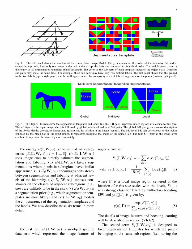
Fig. 1. The left panel shows the structure of the Hierarchical Image Model. The grey circles are the nodes of the hierarchy. All nodes,except the top node, have only one parent nodes. All nodes except the leafs are connected to four child nodes. The middle panel shows adictionary of 30 segmentation templates (hand designed). The color of the sub-parts of each template indicates the object class. Differentsub-parts may share the same label. For example, three sub-parts may have only two distinct labels. The last panel shows that the groundtruth pixel labels (upper right panel) can be well approximated by composing a set of labeled segmentation templates (bottom right panel).

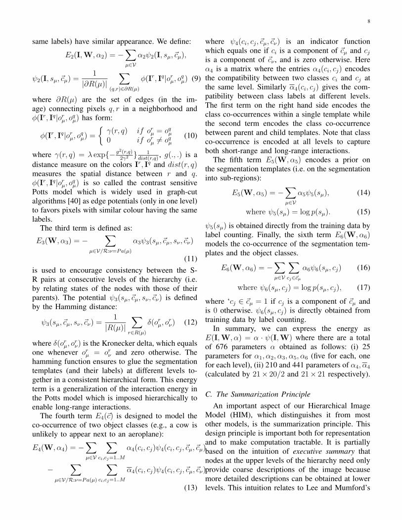
Fig. 2. This figure illustrates how the segmentation templates and labels (i.e. the S-R pairs) represent image regions in a coarse-to-fine way.The left figure is the input image which is followed by global, mid-level and local S-R pairs. The global S-R pair gives a coarse descriptionof the object identity (horse), its background (grass), and its position in the image (central). The mid-level S-R pair corresponds to the regionbounded by the black box in the input image. It represents (roughly) the shape of the horse’s leg. The four S-R pairs at the lower levelcombine to represent the same leg more accurately.

The energy E(I,W, α) is the sum of six energyterms {Ei(I,W, α) : i = 1, .., 6}: (i) E1(I,W, α1)uses image cues to directly estimate the segmen-tation and labeling, (ii) E2(I,W, α2) favors seg-mentations where pixels in subregions have similarappearance, (iii) E3(W, α3) encourages consistencybetween segmentation and labeling at adjacent lev-els of the hierarchy, (iv) E4(W, α4) imposes con-straints on the classes of adjacent sub-regions (e.g.,cows are unlikely to be in the sky), (v) E5(W, α5) isa segmentation prior (e.g., which segmentation tem-plates are most likely), and (vi) E6(W, α6) modelsthe co-occurrence of the segmentation templates andthe labels. We now describe these six terms in moredetail.

The first term E1(I,W, α1) is an object specificdata term which represents the image features of

regions. We set:

E1(I,W, α1) = −∑µ∈V

α1ψ1(I, sµ,~cµ)

with ψ1(I, sµ,~cµ) =1

|R(µ)|∑

r∈R(µ)

log p(orµ|Ir) (7)

where Ir is a local image region centered at thelocation of r (its size scales with the level), F (·, ·)is a (strong) classifier learnt by multi-class boosting[39] and p(or

µ|Ir) is given by:

p(orµ|Ir) =

exp{F (Ir, orµ)}∑

o′ exp{F (Ir, o′)} (8)

The details of image features and boosting learningwill be described in section (VI-A2).

The second term E2(I,W, α2) is designed tofavor segmentation templates for which the pixelsbelonging to the same sub-regions (i.e., having the

8

same labels) have similar appearance. We define:

E2(I,W, α2) = −∑µ∈V

α2ψ2(I, sµ,~cµ),

ψ2(I, sµ,~cµ) =1

|∂R(µ)|∑

(q,r)∈∂R(µ)

φ(Ir, Iq|orµ, o

qµ) (9)

where ∂R(µ) are the set of edges (in the im-age) connecting pixels q, r in a neighborhood andφ(Ir, Iq|or

µ, oqµ) has form:

φ(Ir, Iq|orµ, o

qµ) =

{γ(r, q) if or

µ = oqµ

0 if orµ 6= oq

µ(10)

where γ(r, q) = λ exp{−g2(r,q)2γ2 } 1

dist(r,q), g(., .) is a

distance measure on the colors Ir, Iq and dist(r, q)measures the spatial distance between r and q.φ(Ir, Iq|or

µ, oqµ) is so called the contrast sensitive

Potts model which is widely used in graph-cutalgorithms [40] as edge potentials (only in one level)to favors pixels with similar colour having the samelabels.

The third term is defined as:

E3(W, α3) = −∑

µ∈V/R:ν=Pa(µ)

α3ψ3(sµ,~cµ, sν ,~cν)

(11)is used to encourage consistency between the S-R pairs at consecutive levels of the hierarchy (i.e.by relating states of the nodes with those of theirparents). The potential ψ3(sµ,~cµ, sν ,~cν) is definedby the Hamming distance:

ψ3(sµ,~cµ, sν ,~cν) =1

|R(µ)|∑

r∈R(µ)

δ(orµ, o

rν) (12)

where δ(orµ, o

rν) is the Kronecker delta, which equals

one whenever orµ = or

ν and zero otherwise. Thehamming function ensures to glue the segmentationtemplates (and their labels) at different levels to-gether in a consistent hierarchical form. This energyterm is a generalization of the interaction energy inthe Potts model which is imposed hierarchically toenable long-range interactions.

The fourth term E4(~c) is designed to model theco-occurrence of two object classes (e.g., a cow isunlikely to appear next to an aeroplane):

E4(W, α4) = −∑µ∈V

∑ci,cj=1..M

α4(ci, cj)ψ4(ci, cj,~cµ,~cµ)

−∑

µ∈V/R:ν=Pa(µ)

∑ci,cj=1..M

α4(ci, cj)ψ4(ci, cj,~cµ,~cν)

(13)

where ψ4(ci, cj,~cµ,~cν) is an indicator functionwhich equals one if ci is a component of ~cµ and cj

is a component of ~cν , and is zero otherwise. Hereα4 is a matrix where the entries α4(ci, cj) encodesthe compatibility between two classes ci and cj atthe same level. Similarly α4(ci, cj) gives the com-patibility between class labels at different levels.The first term on the right hand side encodes theclass co-occurrences within a single template whilethe second term encodes the class co-occurrencebetween parent and child templates. Note that classco-occurrence is encoded at all levels to captureboth short-range and long-range interactions.

The fifth term E5(W, α5) encodes a prior onthe segmentation templates (i.e. on the segmentationinto sub-regions):

E5(W, α5) = −∑µ∈V

α5ψ5(sµ), (14)

where ψ5(sµ) = log p(sµ). (15)

ψ5(sµ) is obtained directly from the training data bylabel counting. Finally, the sixth term E6(W, α6)models the co-occurrence of the segmentation tem-plates and the object classes.

E6(W, α6) = −∑µ∈V

∑

cj∈~cµ

α6ψ6(sµ, cj) (16)

where ψ6(sµ, cj) = log p(sµ, cj), (17)

where ‘cj ∈ ~cµ = 1 if cj is a component of ~cµ andis 0 otherwise. ψ6(sµ, cj) is directly obtained fromtraining data by label counting.

In summary, we can express the energy asE(I,W, α) = α · ψ(I,W) where there are a totalof 676 parameters α obtained as follows: (i) 25parameters for α1, α2, α3, α5, α6 (five for each, onefor each level), (ii) 210 and 441 parameters of α4, α4

(calculated by 21× 20/2 and 21× 21 respectively).

C. The Summarization PrincipleAn important aspect of our Hierarchical Image

Model (HIM), which distinguishes it from mostother models, is the summarization principle. Thisdesign principle is important both for representationand to make computation tractable. It is partiallybased on the intuition of executive summary thatnodes at the upper levels of the hierarchy need onlyprovide coarse descriptions of the image becausemore detailed descriptions can be obtained at lowerlevels. This intuition relates to Lee and Mumford’s

9

[41] high resolution buffer hypothesis for the visualcortex.

The summarization principle has four aspects.(I) The state of wν the random variable at node

ν ∈ V/VLEAF is a summary of the state of itschild nodes µ ∈ Ch(ν), and hence summarizes theirstates, see figure (2).

(II) The representational complexity of a nodeis the same at all levels of the tree – the randomvariables are restricted to take the same number ofstates.

(III) The clique potentials for a node ν ∈ Vdepends on its parent nodes and it child nodes, butnot on its grandparents or grandchildren. This is aMarkov property on the hierarchy. But, as will bedescribed later, all nodes can receive input directlyfrom the input image.

(IV) The potentials defined over the cliques de-pend only on simple statistics which also summarizethe states of the child nodes.

The executive summary intuition is enforced byaspects (I) and (II) – the upper levels nodes canonly give coarse descriptions of the large imageregions that they represent and these descriptions arebased on the, more detailed, descriptions given bythe lower level nodes. The other two aspects – (III)and (IV) – help reduce the number of cliques in thegraph and restrict the complexity of the potentialsdefined over the cliques. Taken all together, the fouraspects make learning and inference computation-ally practical because of (i) the small clique size, (ii)the simplicity of the potentials, and (iii) the limitedsize of the state space.

IV. INFERENCE: PARSING BY DYNAMICPROGRAMMING

Parsing an image is performed as inference of theHIM. We parse the image by inferring the maximuma posterior (MAP) estimator of the HIM:

W∗ = arg maxW

p(W|I; α) = arg minW

E(I,W, α)

(18)

This will output state variables W∗ = {w∗µ =

(s∗µ,~c∗µ) : µ ∈ V} at all levels of the hierarchy. But

we only use the state variables at the lowest level ofthe graph when we evaluate the HIM for labeling.

The graph of the HIM has no closed loops so Dy-namic Programming (DP) can be applied to calcu-late the best parse tree W ∗ from equation (18). But

the computational complexity is high because of thelarge size of the state space. To see this, observe thatthe number of states at each node is O(MK |Ds|)(where K = 3,M = 21, |Ds| = 30) and sothe computational complexity is O(M2K |Ds|2H)where H is the number of edges in the hierarchy.Note that the choice of our representation, in par-ticular the segmentation-recognition template, hasrestricted the size of the state space by requiring thatnode µ can only assign labels or

µ consistent with thestate wµ = (sµ,~cµ). Nevertheless, the computationalcomplexity means that DP is still impractical onstandard PCs. We hence use a pruned version ofDP which will describe below.

A. Recursive Energy Formulation

The hierarchical form of the HIM (without closedloops) means that the energy term E(I,W, α) canbe computed recursively which will enable DynamicProgramming with pruning.

We can formulate the energy function recursivelyby defining an energy function Eν(I,wdes(ν), α)over the subtree with root node ν in terms of thestate variables wdes(ν) of the subtree, where des(ν)stands for the set of descendent nodes of ν – i.e.wdes(ν) = {wµ : µ ∈ Vν}, where Vν is the subtreewith root node ν.

This can be computed recursively by:

Eν(I,wdes(ν), α) = αdataν · ψdata

ν (I, wν)

+∑

ρ∈Ch(ν)

{Eρ(I,wdes(ρ), α) + αintν · ψint

ν (wν , wρ)},

(19)

where the data terms αdataν · ψdata are

α1ψ1, α2ψ2, α5ψ5, α6ψ6 (i.e. the terms insection (III-B) that depend only on node νand the data I) and the inter-level terms αint

ν · ψintν

are α3ψ3, α4ψ4 (i.e. the terms in section (III-B) thatdepend on node ν and its children Ch(ν)).

By evaluating Eν(I,wdes(ν), α) at the root nodeswe obtain the full energy of the model E(I,W, α).

B. Dynamic Programming with Pruning

We can use the recursive formulation of theenergy, see equation (19), to perform DynamicProgramming. But to ensure rapid inference we willneed to perform pruning by not exploring partial

10

state configurations which seem unpromising. Wefirst describe DP and then give our pruning strategy.

DP proceeds by evaluating possible states wν

for nodes ν of the graph. We will refer to thesepossible states as proposals and denote them by{wν,bν}, where bν indexes the proposals for nodeν. Each proposal is associated with a minimumenergy Emin(wν,bν ) which corresponds to the lowestpossible energy of the subtree whose root node νtakes state wν,bν . More precisely, consider the setof all possible state variables {wdes(ν),bν} for thesubtree with state wν,bν at the root node ν. Then setEmin(wν,bν ) = minwdes(ν),bν

Eν(I,wdes(ν),bν , α).Recursion for parent nodes: for each parent node

µ we first access the proposals {wρ,bρ} for its childnodes ρ ∈ Ch(µ) and their minimum energies{Emin(wρ,bρ)}. Then for each state wµ,bµ of µ, wecompute its minimum energy by solving:

Emin(wµ,bµ) = αdataµ · ψdata

µ (I, wµ,bµ)

+∑

ρ∈Ch(µ)

minwρ,bρ

{Emin(wρ,bρ) + αintµ · ψint

µ (wµ,bµ , wρ,bρ)}

(20)The initialization is performed at the leaf nodes

using the data terms only (E1 and E2).The pruning strategy rejects proposals whose

energies are too high and which hence are unlikelyto lead to the optimal solution. To understand ourpruning strategy, recall that the set of of region par-titions is divided into three subsets S1, S2, S3, whereSi contains partitions with i regions. There are |C|ipossible labels c for each region partition whichgives a very large state space (since |C| = 30).Our pruning strategy is to restrict the set of labels~c allowed for each of these subsets. For subset S1,there is only one region so we allow all possiblelabels for it c1 ∈ C and perform no pruning. Forsubset S2, there are two subregions and we keeponly the best 10 labels for each subregion – i.e. atotal of 10 × 10 = 100 labels (‘best’ means lowestenergy). For subset S3, we keep only the best 5labels of each subregion (hence a total of 53 = 125labels). In summary, when computing the proposalsfor node µ, we group the proposals into three setsdepending on the partition label sµ of the proposal.If sµ ∈ S1, then the proposal is kept. If sµ ∈ S2

or sµ ∈ S3, we keep the top 100 and 125 proposalsrespectively. (We experimented with changing thesenumbers – 100 and 125 – but noticed no significantdifference in performance for small changes).

The top-down pass is used to find the stateconfigurations {WR,b} of the graph nodes VRwhich correspond to the proposals {wR,b} for theroot nodes. By construction, the energies of theseconfigurations is equal to the minimum energies atthe root nodes, see equation (20). This top-downpass recursively inverts equation (20) to obtain thestates of the child nodes that yield the minimumenergy – i.e., it solves:

{w∗ρ : ρ ∈ Ch(µ)} = arg min

{wρ,bρ}{αdata

µ · ψdataµ (I, w∗

µ)

+∑

ρ∈Ch(µ)

{Emin(wρ,bρ) + αintµ · ψint

µ (w∗µ, wρ,bρ)}},(21)

which reduces to:

w∗ρ = arg min

wρ,bρ

{Emin(wρ,bρ)+αintµ ·ψint

µ (w∗µ, wρ,bρ)}.

(22)We then set the optimal solution to be:

W∗ = {w∗µ : µ ∈ V} (23)

V. LEARNING THE MODEL

There are a range of different learning algorithmsthat we could use to estimate the parameters α ofan HIM. These include maximum likelihood, asused in Conditional Random Fields (CRFs) [14],max-margin learning [42], and structure-perceptronlearning [17].

In this paper, we use structure perceptron be-cause of its simplicity (and our previous experienceof using it in [43]). Structure-perceptron learningis simple to implement and only requires us tocalculate the most probable configurations (parses)of the model, see figure (3). By contrast, max-imum likelihood learning requires calculating theexpectation of features which is difficult due to thelarge states of HIM. Moreover, Collins [17] provedtheoretical results for convergence properties, forboth separable and non-separable cases, and alsofor generalization. The structure-perceptron learningwill not compute the partition function Z(I; α) sowe do not have a formal probabilistic interpretation.

The goal of structure-perceptron learning is tolearn a mapping from inputs to output structures. Inour case, the inputs {Ii} are a set of images, and theoutputs {Wi} are a set of parse trees which specifythe labels of image regions in a hierarchical form(in practice, the training set only contains the labelsof the pixels and we perform an approximation

11

to estimate the full parse Wi for the training set,see the implementation details in the ExperimentalResults section). We use a set of training examples{(Ii,Wi) : i = 1...N} and the feature functionsψ(I,W) ∈ Rd described in section (III-B).

The basic structure-perceptron algorithm is de-signed to minimize the loss function:

Loss(α) = α · ψ(I,W)−maxW

α · ψ(I,W), (24)

where W is the correct parse for input I, andW is a dummy variable. We use “the averagedparameters” version whose pseudo-code is givenin figure (3). The algorithm proceeds in a simpleway (similar to the perceptron algorithm for binaryclassification). The parameters are initialized to zeroand the algorithm loops over the training examples.If the highest scoring parse tree for input I isnot correct, then the parameters α are updated byan additive term. The most difficult step of themethod is finding W∗ = arg maxW α · ψ(Ii,W),which can be solved by the inference algorithmfrom section (IV). Hence the computational effi-ciency of structure perceptron (and its practicality)depends on the inference algorithm. As discussedearlier, see section (IV), the inference algorithm haspolynomial computational complexity for an HIMwhich makes structure-perceptron learning practicalfor HIM. The averaged parameters are defined to beγ =

∑Tt=1

∑Ni=1 αt,i/NT , where T is the number of

epochs, NT is the total number of iterations. It isstraightforward to store these averaged parametersand output them as the final estimates.

VI. EXPERIMENTAL RESULTS

We evaluate the segmentation performance of theHIM on two public datasets, i.e. the MSRC 21-classimage datset [16] and the PASCAL VOC 2007[18].

A. Experiment I: MSRC

1) Implementation details: The MSRC dataset isdesigned to evaluate scene labeling including bothimage segmentation and multi-class object recogni-tion. The ground truth only gives the labeling ofthe image pixels. To supplement this ground truthfor learning, we estimate the true labels (i.e. thestates of the S-R pair ) of the nodes in the five-level hierarchy of HIM by selecting the S-R pairs

which have maximum overlap with the labels ofthe image pixels. This approximation only results in2% error in labeling image pixels – this is for thelowest 27× 27 block – and shows that the quadtreerepresentation does not cause too many artifacts.There are a total of 591 images. We use the identicalsplitting as [16], i.e., 45% for training, 10% for val-idation, and 45% for testing. The parameters learntfrom the training set, with the best performance onvalidation set, are selected. This was used to set thenumber of steps of the structure perceptron learningalgorithm.

For a given image I, the parsing result is obtainedby estimating the best configuration W∗ of the HIM.To evaluate the performance of parsing we use theglobal accuracy measured in terms of all pixelsand the average accuracy over the 21 object classes(global accuracy pays most attention to frequentlyoccurring objects and penalizes infrequent objects).A computer with 8 GB memory and 2.4 GHz CPUwas used for training and testing.

2) Image features and potential learning: Theimage features used by the classifier (47 in total) arethe greyscale intensity, the color (R,G, B channels),the intensity gradient, the Canny edge, the responseof DOG (difference of Gaussians) and DOOG (Dif-ference of Offset Gaussian) filters at different scales(13*13 and 22*22) and orientations (0,30,60,...),and so on. We use 55 types of shape (spatial) filters(similar to [16]) to calculate the responses of 47image features. There are 2585 = 47 ∗ 55 featuresin total. For each class, there are around 4, 500weak classifiers selected by multi-class boosting.The boosting learning takes about 35 hours of which27 hours are spent on I/O processing and 8 hourson computing.

3) Parsing results: The segmentation perfor-mance of the HIM on the MSRC dataset is shownin table (II). The confusion matrix of 21 objectclasses is shown in figure (4) where the diagonalentries give the classification accuracy of individualclasses. Figure (5) (best viewed in color) showssome parsing results obtained by the HIM and bythe E1(I,W, α) classifier term alone (i.e. p(or

µ|I)).Observe that the HIM gives better results than theclassifier term alone and hence justifies the use ofthe hierarchy in order to ensure long-range interac-tions – see improvements of 20% and 32% in rows 6and 7. This improvement is quantified in Table (II)showing that HIM improves the results obtained by

12

Input: A set of training images with ground truth (Ii,Wi) for i = 1..N . Initialize parametervector α = 0.For t = 1..T, i = 1..N

• find the best state of the model on the i’th training image with current parameter setting,i.e., W∗ = arg maxW α · ψ(Ii,W)

• Update the parameters: α = α + ψ(Ii,Wi)− ψ(Ii,W∗)• Store: αt,i = α

Output: Parameters γ =∑

t,i αt,i/NT

Fig. 3. The structure-perceptron learning algorithm. α and ψ(I,W) represent all the parameters and factor functions from section (III-B).

the classifier by 6.9% for average accuracy and 5.3%for global accuracy. Observe also, from figure (5),that the HIM is able to roughly capture segmentationboundaries of different types of regions (e.g., cowlegs, sky boundaries, etc.). Observe that the resultslook slightly ‘blocky’ due to the limited number ofsegmentation templates.

4) Performance comparisons: In table (II), wecompare the performance of our approach with othersuccessful methods [16], [44], [45]. Our approachoutperforms those alternatives by 6% in averageaccuracy and 4% in global accuracy. Our boostingresults are better than Textonboost [16] because ofour choice of image features. This raises a question– would we get better results if we used a flat CRFinstead of an HIM but with the same image features?We argue that we would not because the CRF onlyimproves TextonBoost’s performance by 3% [16],while we gain 5% by using the hierarchy (and westart with a higher baseline). Some other methods[46], [31], [15], which are worse than [44], [45] andevaluated on simpler datasets [15], [31] (less than 10classes), are not listed here due to lack of space. Wealso report recent progress [47], [48] on this dataset(only available after our paper was submitted forreview). In particular, Ladicky et al.[48] achievesbetter performance – 86% compared to our 81.4%– probable because they use more powerful unaryclassifiers, see table (II), and also adaptive imagepartitioning.

5) Empirical convergence analysis of perceptronlearning.: The structure-perceptron learning algo-rithm takes about 20 hours to converge in 5520 (T =20, N = 276) iterations. In the testing stage, ittakes 30 seconds to parse an image of 320× 200 (6seconds for extracting image features, 9 seconds forcomputing the strong classifier of boosting and 15seconds for parsing the HIM). Figure (6) plots the

����������������������������� � � �� ��� �� ���� ����������������� � !�� " #$%&�$ � !�� "

Fig. 6. Empirical Convergence Analysis on the MSRC dataset.The curves plot the average and global accuracy as a function ofthe number of iterations (of parameter estimation). The accuracy isevaluated on the test dataset

convergence curves evaluated by average accuracyand global accuracy on the test set. It shows thatstructure-perceptron converges in T = 20 epochs.

6) Object part detection by S-R pairs.: Figure (7)shows how the S-R pairs can be used to detect partsof objects. For example, the S-R pair consisting oftwo horizontal bars labeled “cow” and “grass” re-spectively indicates the cow’s stomach consistentlyacross different images. Similarly, the cow’s tail canbe located according to the configuration of anotherS-R pair with vertical bars. These results are onlyapproximate but they show proof of concept. Infuture research we will develop this idea in orderto parse objects into their constituent parts.

B. Experiment II: PASCAL VOC 2007The PASCAL VOC 2007 dataset [18] was used

for the PASCAL Visual Object Category segmen-tation contest 2007. It contains 209 training, 213validation and 210 segmented test images of 20foreground (object) and 1 background classes. Itis more challenging than the MSRC-21 dataset dueto more significant background clutter, illumination

13

Fig. 4. The confusion matrix for object classes evaluated on the MSRC dataset [16].

Textonboost[16] PLSA-MRF [44] Auto-context [45] Region Ancestry[47] HCRF[48] Classifier only HIMAverage 57.7 64.0 68 67 75 (72) 67.2 74.1Global 72.2 73.5 77.7 – 86 (81) 75.9 81.2

TABLE IIPERFORMANCE COMPARISONS FOR AVERAGE ACCURACY AND GLOBAL ACCURACY ON THE MSRC DATASET. “CLASSIFIER ONLY” ARE

THE RESULTS WHERE THE PIXEL LABELS ARE PREDICTED BY THE CLASSIFIER OBTAINED BY BOOSTING ONLY (THE E1(I,W, α)TERM). THE NUMBERS IN THE BRACKETS ARE THE RESULTS OBTAINED BY THE CLASSIFIER (UNARY POTENTIAL) USED IN HCRF [48].

Brookes TKK UoCTTI HIMAverage 8.5 30.4 21.2 26.5Global 58.4 24.4 – 67.2

TABLE IIIPERFORMANCE COMPARISONS ON THE PASCAL VOC 2007

DATASET. THREE METHODS REPORTED IN THE VOCSEGMENTATION CONTEST 2007 [18] ARE COMPARED.

effects and occlusions. We trained the HIM usingthe same parameter settings and features as in theexperiment on the MSRC-21 dataset. Some parseresults are shown in figure (8). The segmentedresults look visually worse than those on the MSRCdataset because in the PASCAL dataset, a single“background” class covers several object classes,such as sky, grass, etc. while more accurate labelingis imposed in the MSRC dataset. We compared ourapproach with other representative methods reportedin the PASCAL VOC segmentation contest 2007[18]. The comparisons in table (III) show that theHIM outperforms most methods and is comparablewith TKK. We note that [49] obtains better results –73.5 % correct – but they only gets 65.0 % correcton MSRC.

VII. CONCLUSION

This paper describes a novel hierarchical imagemodel (HIM) for 2D image parsing. The hierarchi-cal nature of the model, and the use of recursivesegmentation and recognition templates, enables theHIM to represent complex image structures in acoarse-to-fine manner. We can perform inference(parsing) rapidly in polynomial time by exploit-ing the hierarchical structure. Moreover, we canlearn the HIM probability distribution from labeledtraining data by adapting the structure-perceptronalgorithm. We demonstrated the effectiveness ofHIM’s by applying them to the challenging task ofsegmentation and labeling of the public MSRC andPASCAL VOC 2007 image databases. Our resultsshow that we perform competitively with state-of-the-art approaches.

The design of the HIM was motivated by drawingparallels between language and vision processing.We have attempted to capture the underlying spiritof the successful language processing approaches– the hierarchical representations based on the re-cursive composition of constituents and efficientinference and learning algorithms. Our current work

14

Fig. 5. This figure is best viewed in color. The colors indicate the labels of 21 object classes as in the MSRC dataset [16]. The columns(except the fourth “numerical accuracy” column) show the input images, ground truth, the labels obtained by HIM and the boosting classifierrespectively. The “numerical accuracy” column shows the global accuracy obtained by HIM (left) and the classifier alone (right). In these 7examples, HIM improves the classifier by 1%, -1% (an outlier!), 1%, 10%, 18%, 20% and 32% in terms of global accuracy.

attempts to extend the HIM’s to improve their repre-sentational power while maintaining computationalefficiency.

ACKNOWLEDGMENTS

This research was supported by the W.M. Keckfoundation, NSF grants 0413214 and 613563, andby the Air Force FA9550-08-1-0489. Part of thisresearch was supported by WCU (World Class

University) program through the National ResearchFoundation of Korea funded by the Ministry ofEducation, Science and Technology(R31-2008-000-10008-0).

REFERENCES

[1] F. Jelinek and J. D. Lafferty, “Computation of the probabilityof initial substring generation by stochastic context-free gram-mars,” Computational Linguistics, vol. 17, no. 3, pp. 315–323,1991.

15

Fig. 7. The S-R pairs can be used to identify (roughly) different parts of objects. Colors indicate the object identities. Observe that thesame S-R pairs (e.g., stomach above grass, and tail to the left of grass) correspond to the same object part in different images.

Fig. 8. Parse results on the PASCAL VOC 2007 dataset [18]. The first three columns show the input images, the groundtruth and the parseresults of HIM, respectively. The next three columns show the other four examples.

[2] M. Collins, “Head-driven statistical models for natural languageparsing,” Ph.D. Thesis, University of Pennsylvania, 1999.

[3] K. Lari and S. J. Young, “The estimation of stochastic context-free grammars using the inside-outside algorithm,” in ComputerSpeech and Languag, 1990.

[4] M. Shilman, P. Liang, and P. A. Viola, “Learning non-generativegrammatical models for document analysis,” in Proceedings ofIEEE International Conference on Computer Vision, 2005, pp.962–969.

[5] Z. Tu and S. C. Zhu, “Image segmentation by data-drivenmarkov chain monte carlo,” IEEE Transactions on PatternAnalysis and Machine Intelligence, vol. 24, no. 5, pp. 657–673,2002.

[6] Z. Tu, X. Chen, A. L. Yuille, and S. C. Zhu, “Image parsing:Unifying segmentation, detection, and recognition,” in Proceed-ings of IEEE International Conference on Computer Vision,2003, pp. 18–25.

[7] Y. Jin and S. Geman, “Context and hierarchy in a probabilisticimage model,” in Proceedings of IEEE Computer Society Con-ference on Computer Vision and Pattern Recognition, 2006, pp.

2145–2152.[8] S. Zhu and D. Mumford, “A stochastic grammar of images,”

Foundations and Trends in Computer Graphics and Vision,vol. 2, no. 4, pp. 259–362, 2006.

[9] C. Bouman and M. Shapiro, “A multiscale random field modelfor Bayesian image segmentation,” IEEE Trans. Image Process-ing, vol. 3, no. 2, pp. 162–177, Mar. 1994.

[10] M. S. Crouse, R. D. Nowak, and R. G. Baraniuk, “Wavelet–based statistical signal processing using hidden Markov mod-els,” IEEE Trans. Signal Processing, vol. 46, no. 4, pp. 886–902, Apr. 1998.

[11] C. Spence, L. C. Parra, and P. Sajda, “Varying complexity intree–structured image distribution models,” IEEE Trans. ImageProcessing, vol. 15, no. 2, pp. 319–330, Feb. 2006.

[12] J. J. Kivinen, E. B. Sudderth, and M. I. Jordan, “Learningmultiscale representations of natural scenes using Dirichletprocesses,” in ICCV, 2007.

[13] A. S. Willsky, “Multiresolution Markov models for signal andimage processing,” Proc. of the IEEE, vol. 90, no. 8, pp. 1396–1458, Aug. 2002.

16

[14] J. D. Lafferty, A. McCallum, and F. C. N. Pereira, “Conditionalrandom fields: Probabilistic models for segmenting and labelingsequence data,” in Proceedings of International Conference onMachine Learning, 2001, pp. 282–289.

[15] X. He, R. S. Zemel, and M. A. Carreira-Perpinan, “Multiscaleconditional random fields for image labeling,” in Proceedingsof IEEE Computer Society Conference on Computer Vision andPattern Recognition, 2004, pp. 695–702.

[16] J. Shotton, J. M. Winn, C. Rother, and A. Criminisi, “Texton-Boost: Joint appearance, shape and context modeling for multi-class object recognition and segmentation,” in Proceedings ofEuropean Conference on Computer Vision, 2006, pp. 1–15.

[17] M. Collins, “Discriminative training methods for hidden markovmodels: theory and experiments with perceptron algorithms,” inProceedings of Annual Meeting on Association for Computa-tional Linguistics conference on Empirical methods in naturallanguage processing, 2002, pp. 1–8.

[18] E. M., L. Van Gool, C. K. I. Williams, J. Winn,and A. Zisserman, “The PASCAL Visual Object ClassesChallenge 2007 (VOC2007) Results,” http://www.pascal-network.org/challenges/VOC/voc2007/workshop/index.html.

[19] L. Zhu, Y. Chen, Y. Lin, C. Lin, and A. Yuille, “Recursivesegmentation and recognition templates for 2d parsing,” inAdvances in Neural Information Processing Systems, 2008.

[20] S. Geman and D. Geman, “Stochastic relaxation, gibbs distri-butions, and the bayesian restoration of images,” IEEE Trans-actions on Pattern Analysis and Machine Intelligence, 1984.

[21] A. Blake and A. Zisserman, Visual Reconstruction. MIT Press,1987.

[22] D. Mumford and J. Shah, “Optimal approximations of piece-wise smooth functions and associated variational problems,” inComm. in Pure and Appl. Math., 1989.

[23] D. Geiger and F. Girosi, “Parallel and deterministic algorithmsfrom mrfs: Surface reconstruction,” IEEE Trans. on PatternAnalysis and Machine Intelligence, 1991.

[24] D. Geiger and A. Yuille, “A common framework for imagesegmentation,” International Journal of Computer Vision, 1991.

[25] C. Koch, J. Marroquin, and A. Yuille, “Analog neuronal net-works in early vision,” in Proceedings of the National Academyof Science, 1986.

[26] S. C. Zhu, Y. N. Wu, and D. Mumford, “Minimax entropyprinciple and its application to texture modeling,” Neural Com-putation, vol. 9, no. 8, pp. 1627–1660, 1997.

[27] S. Roth and M. Black, “Fields of experts: A framework forlearning image priors,” in Proceedings of the IEEE Conferenceon Computer Vision and Pattern Recognition, 2005.

[28] S. Konishi, A. L. Yuille, J. M. Coughlan, and S. C. Zhu,“Statistical edge detection: Learning and evaluating edge cues,”IEEE Trans.on Pattern Analysis and Machine Intelligence,2003.

[29] A. Rosenfeld, R. A. Hummel, and S. W. Zucker, “Scene labelingby relaxation operations,” IEEE Trans. Syst., Man, Cybern,1976.

[30] S. Kumar and M. Hebert, “Discriminative random fields: Adiscriminative framework for contextual interaction in classifi-cation,” in International Conference on Computer Vision, 2003.

[31] ——, “A hierarchical field framework for unified context-based classification,” in Proceedings of IEEE InternationalConference on Computer Vision, 2005, pp. 1284–1291.

[32] A. Levin and Y. Weiss, “Learning to combine bottom-up andtop-down segmentation,” in Proceedings of European Confer-ence on Computer Vision, 2006, pp. 581–594.

[33] P. J. Cowans and M. Szummer, “A graphical model for simul-taneous partitioning and labeling,” in Proceedings of AI andStatistics, 2005.

[34] S. Zhu and A. Yuille, “Region competition: Unifyingsnake/balloon, region growing and bayes/mdl/energy for multi-band image segmentation,” IEEE Trans. on Pattern Analysisand Machine Intelligence, 1996.

[35] H. Chen, Z. Xu, Z. Liu, and S. C. Zhu, “Composite templatesfor cloth modeling and sketching,” in Proceedings of IEEEComputer Society Conference on Computer Vision and PatternRecognition, 2006, pp. 943–950.

[36] E. B. Sudderth, A. B. Torralba, W. T. Freeman, and A. S.Willsky, “Learning hierarchical models of scenes, objects, andparts,” in Proceedings of IEEE International Conference onComputer Vision, 2005, pp. 1331–1338.

[37] E. Sharon, A. Brandt, and R. Basri, “Fast multiscale imagesegmentation,” in Proceedings of IEEE Computer Society Con-ference on Computer Vision and Pattern Recognition, 2000, pp.1070–1077.

[38] T. Cour, F. Benezit, and J. Shi, “Spectral segmentation withmultiscale graph decomposition,” in Proceedings of IEEE Com-puter Society Conference on Computer Vision and PatternRecognition, 2005.

[39] E. L. Allwein, R. E. Schapire, and Y. Singer, “Reducing mul-ticlass to binary: A unifying approach for margin classifiers,”Journal of Machine Learning Research, vol. 1, pp. 113–141,2000.

[40] Y. Boykov and M.-P. Jolly, “Interactive graph cuts for optimalboundary and region segmentation of objects in n-d images,”in Proceedings of IEEE International Conference on ComputerVision, 2001, pp. 105–112.

[41] T. Lee and D. Mumford, “Hierarchical bayesian inference inthe visual cortex,” Journal of the Optical Society of America,2003.

[42] B. Taskar, D. Klein, M. Collins, D. Koller, and C. Manning,“Max-margin parsing,” in Proceedings of Annual Meeting onAssociation for Computational Linguistics conference on Em-pirical methods in natural language processing, 2004.

[43] L. Zhu, Y. Chen, X. Ye, and A. L. Yuille, “Structure-perceptronlearning of a hierarchical log-linear model,” in Proceedings ofIEEE Computer Society Conference on Computer Vision andPattern Recognition, 2008.

[44] J. Verbeek and B. Triggs, “Region classification with markovfield aspect models,” in Proceedings of IEEE Computer SocietyConference on Computer Vision and Pattern Recognition, 2007.

[45] Z. Tu, “Auto-context and its application to high-level visiontasks,” in Proceedings of IEEE Computer Society Conferenceon Computer Vision and Pattern Recognition, 2008.

[46] J. Verbeek and B. Triggs, “Scene segmentation with crfs learnedfrom partially labeled images,” in Advances in Neural Informa-tion Processing Systems, vol. 20, 2008.

[47] J. J. Lim, P. Arbelaez, C. Gu, and J. Malik, “Context by re-gion ancestry,” in IEEE International Conference on ComputerVision, 2009.

[48] L. Ladicky, C. Russell, P. Kohli, and P. Torr, “Associativehierarchical crfs for object class image segmentation,” in IEEEInternational Conference on Computer Vision, 2009.

[49] G. Csurka and F. Perronnin, “A simple high performanceapproach to semantic segmentation,” in Proceedings of BMVC,2008.