recursive neural filters and dynamical range transformers

Recursive Neural Filters and Dynamical RangeTransformers

JAMES T. LO AND LEI YU

Invited Paper

A recursive neural filter employs a recursive neural network toprocess a measurement process to estimate a signal process. Thispaper reviews and presents new results on recursive neural filtersthrough introducing those based on a multilayer perceptron withoutput feedbacks and proposing dynamical range reducers and ex-tenders for applications where the range of the measurement orsignal process expands in time or is too large for the recurrentneural network to handle for the filtering resolution required.

As opposed to the conventional analytic approach to derivingfilter equations, recursive neural filters are synthesized from exem-plary realizations of the signal and measurement processes, whichare obtained by either computer simulations or actual experiments.No assumptions such as linear dynamics, Gaussian distribution, ad-ditive noise, and Markov property are required.

A properly trained recursive neural filter with a proper architec-ture carries the most “informative” statistics in its dynamical stateand approximates the optimal performance to any accuracy. Therecursive neural filter is a massively parallel algorithm ideal forreal-time implementation.

Dynamical range reducers and extenders proposed are prepro-cessors and postprocessors of a recurrent neural network that, re-spectively, reduce the range of the exogenous input and extend thatof the output of the recurrent neural network. While a dynamicalrange reducer reduces the exogenous input range by subtracting anestimate of the exogenous input from it, a dynamical range extenderextends the output range by adding an estimate of the output to it.

Three types of dynamical range reducer by estimate subtractionand five types of dynamical range extender by estimate addition areprovided, which have different levels of effectiveness and computa-tional costs. Selection from the different types for an application isdetermined by the tradeoff between the effectiveness and computa-tional cost.

Two types of dynamical range extender by estimate addition usean extended Kalman filter (EKF) to generate the added estimate.

Manuscript received February 18, 2003; revised October 28, 2003. Thiswork was supported in part by the National Science Foundation underGrants ECS-0114619 and ECS-9707206, in part by the Army ResearchOffice under Contract DAAD19-99-C-0031, and in part by the RomeLaboratory under Contract F30602-91-C0033.

James T. Lo is with the Department of Mathematics and Statistics, Uni-versity of Maryland Baltimore County, Baltimore, MD 21250 USA (e-mail:[email protected]).

Lei Yu is with the Microsoft Corporation, Washington, DC 20015 USA(e-mail: [email protected]).

Digital Object Identifier 10.1109/JPROC.2003.823148

They can be viewed as methods of using a recursive neural filteronly to make up the nonlinear part ignored by the EKF.

Keywords—Dynamical range extender, dynamical rangereducer, Kalman filter (KF), measurement, minimum variance, op-timal filtering, recursive filtering, recursive neural filter, recursiveneural network, signal, synthetic approach.

I. INTRODUCTION

In the standard formulation of the main problem in themodern theory of optimal filtering, the signal process andmeasurement process are described by the mathematical/sta-tistical model

(1)

(2)

where and are -dimensional and -dimensionalstochastic processes, respectively; is a Gaussian randomvector, and are, respectively, -dimensional and

-dimensional Gaussian noise processes with zero means;, and have given joint probability distributions; and

, and are known functions withsuch appropriate dimensions and properties that (1) and (2)describe the evolutions of the signal and measurement.

The problem of discrete-time optimal filtering is todesign and make a discrete-time dynamical system thatinputs and outputs an estimate of at each time

, which minimizes a given estimationerror criterion. Here is a positive integer or infinity. Thedynamical system is called an optimal filter with respectto the given estimation error criterion. The dynamical stateof the optimal filter at a time must carry the optimalconditional statistics given all the measurements thathave been received up to and including the time at thetime so that at the next time , the optimal filter willreceive and process using the optimal conditionalstatistics from , and then produce the optimal estimate

. The most widely used estimation error criterion is

0018-9219/04$20.00 © 2004 IEEE

514 PROCEEDINGS OF THE IEEE, VOL. 92, NO. 3, MARCH 2004

the mean square error criterion , whereand denote the expectation and the Euclidean norm,respectively. The estimate that minimizes this criterion iscalled the minimum-variance estimate.

If and are linear functions of , and does notdepend on , the model, (1) and (2), is called the linear-Gaussian model. A minimum-variance filter is the celebratedKalman filter (KF) [1], [2] described in the first paper in thisspecial issue by S. Haykin. In most real-world applications,however, the foregoing linearity conditions on andare not satisfied and the extended KF (EKF) is used. At eachtime point, the EKF first linearizes and at the estimatedvalue of and linearizes at the predicted value of .Then the EKF uses the KF equations to update the estimatedvalue of and the predicted value of for the newmeasurement . By iterating the linearization and estima-tion a certain number of times or until convergence at eachtime point, we have the so-called iterated EKF (IEKF). Sinceboth the EKF and IEKF involve linearization, they are notoptimal filters. In fact, when either the random driving term

in (1) or the random measurement noise in(2) has such large variances or covariances that the aforemen-tioned estimated value and predicted value of the signal arenot very close to the true signal, or when the functions ,and are not very smooth, linearization may be a poor ap-proximation and the EKF as well as IEKF may yield poor es-timates or even diverge. The reader is referred to S. Haykin’spaper in this special issue for more descriptions and refer-ences for KFs and EKFs.

This shortcomings of the EKF and IEKF have motivatedan enormous amount of work on nonlinear filtering by the an-alytic approach for over 30 years [3]–[5]. (More referencescan be found in the papers by Haykin and Krishnamurthyand Elliott in this special issue.) Starting with a mathemat-ical model, the analytic approach searches for a solution orapproximate solution consisting of equations that describethe structures or characterize the variables of the filter. Inthe process of searching, deductive reasoning is used andmany assumptions are made to make some special cases an-alytically tractable. In fact, the KF was derived under theassumptions that and are linear in does not de-pend on , and and are Gaussian sequences. Thegeneral model, (1) and (2), contains such assumptions as theMarkov property, Gaussian distribution, and additive mea-surement noise.

It is appropriate to mention here that many approximatenonlinear filters have been obtained, which can be viewedas predecessors of the recursive neural filters discussed inthis paper. Among them are those derived by approximatingnon-Gaussian densities with Gaussian sums [6], [7], thoseobtained on group manifolds [8]–[11], and those obtainedby functional series expansion [12]–[16]. These approximatefilters are optimal for the given structure and approach theminimum variance filter as the number of terms increases.These are the properties shared by the recursive neural filters.However, those approximate filters often involve a great dealof computation and/or an excessive number of terms. TheEKF and, to a much less extent, the IEKF remain as the stan-dard filters for estimating stochastic signals in practice.

An alternative approach was proposed in 1992 [17], [18].As opposed to the analytic approach, the proposed approachis synthetic in nature. Instead of deriving equations based ona mathematical model such as (1) and (2), the synthetic ap-proach synthesizes data collected by actual experiments orcomputer simulations into a recursive filter that approximatesa theoretical optimal filter in performance to any preselecteddegree of accuracy with respect to a given estimation crite-rion.

In the synthetic approach, a class of dynamical systemsthat are universal approximators of optimal filters is required.A most parsimonious class of this kind is multilayer percep-trons with interconnected neurons (MLPWINs) used in [17],[19]. The synthesis of a recursive filter is performed throughtraining at least one MLPWIN and selecting one in con-sideration of the filtering performance versus the numbersof nodes and connections in the MLPWIN to optimize thecost-effectiveness. In training an MLPWIN, the adjustableweights (including biases) are determined essentially by min-imizing or reducing a training criterion by the variation ofthem.

A training criterion, which is constructed with thetraining data, is a function of these adjustable weights ofthe MLPWIN under training. The training criterion does nothave to be the standard minimum-variance criterion and canbe defined to reflect an estimation error criterion suitablefor the filtering needs and environment. Since we do notuse a mathematical model of the signal and measurementprocesses to derive equations, such properties as the Markovproperty, Gaussian distribution, and additive noise are notrequired of the signal and measurement processes for thesynthetic approach.

A properly trained MLPWIN with a proper architecture isa virtually optimal recursive filter, whose dynamical state ata time carries the most “informative” conditional statistics[17], [19] at the time for generating subsequent optimal es-timates after the time. The massively parallel architecture ofthe MLPWIN makes it ideal for real-time filtering.

However, there are two shortcomings in using anMLPWIN as a recursive filter. First, if the mean or covari-ance of the initial signal (i.e., signal at time 0) is available,the information cannot be used by the MLPWIN, resultingin a longer and suboptimal transient filter state. Second, ifthe ranges of the signal and measurement expand over time,such as in financial time series prediction, satellite orbitdetermination, aircraft/ship navigation, and target tracking,or are large relative to the filtering resolution or accuracyrequired, the size of the MLPWIN and the training data setmust be large. The larger the MLPWIN and the trainingdata set are, the more difficult it is to train the MLPWINon the training data set. Furthermore, the periods overwhich the training data is collected, by computer simulationor actual experiment, are necessarily of finite length. Ifthe measurement and signal processes grow beyond theseperiods, the MLPWIN trained on the training data usuallydiverges after them.

The main purpose of this paper is to show how these twoshortcomings can be eliminated. Our method of incorpo-rating the mean or covariance of the initial signal is the use

LO AND YU: RECURSIVE NEURAL FILTERS AND DYNAMICAL RANGE TRANSFORMERS 515

of a recursive neural network (RNN) with output feedbackssuch as a multilayer perceptron with output feedbacks(MLPWOF) instead of an MLPWIN. It is proven here thatthe minimum-variance filter can also be approximated toany accuracy by an MLPWOF. The mean or covariance ofthe initial signal can be loaded into the MLPWOF at theoutput feedback terminals before it starts filtering the mea-surements. MLPWOFs are numerically tested as recursivefilters for the same signal and measurement processes as in[17] and [19]. Their filtering performances are shown to besimilar to those of the neural filters with an MLPWIN andsuperior to those of the EKFs and IEKFs.

MLPWINs and MLPWOFs are two types of RNN widelyused. There are other types. For instance, combinations ofthe two often work better. However, we will not discuss theRNN architecture selection further in this paper.

To eliminate the foregoing second difficulty, we proposethe use of dynamical range transformers. There are two typesof dynamical range transformer, called dynamical range re-ducers or extenders, which are preprocessors and postpro-cessors, respectively, of an RNN. A dynamical range reducertransforms dynamically a component of an exogenous inputprocess (e.g., a measurement process) and sends the resultingprocess to the input terminals of an RNN so as to reduce thevalid input range or approximation capability required of theRNN. On the other hand, a dynamical range extender trans-forms dynamically the output of an output node of an RNNso as to reduce the valid output range or approximation capa-bility required of the RNN. The purpose of both the dynam-ical range reducer and extender is to ease the RNN size andtraining data requirements and thereby lessen the training dif-ficulty. The fundamental range transforming requirement inusing a dynamical range transformer (i.e., dynamical rangereducer or extender) is the existence of a recursive filter com-prising an RNN and the dynamical range transformer that ap-proximates the optimal filter to any accuracy, provided thatthe RNN with the selected architecture is sufficiently large.A recursive filter comprising an RNN and dynamical rangetransformers is called a recursive neural filter.

A basic scheme to reduce the measurement range is tosubtract an estimate of the current measurement from thecurrent measurement, the estimate being based on measure-ments preceding the current measurement. A type of dynam-ical range reducer using this scheme are called range reducersby estimate subtraction. Three types of range reducer by es-timate subtraction—namely, range reducers by differencing,range reducers by linear prediction, and range reducers bymodel-aided prediction—are introduced.

If the signal process is observable from the outputs of thedynamical range reducers in a recursive neural filter or if themean and covariance of the initial signal are fixed, a recursiveneural filter consisting of an MLPWIN or MLPWOF and dy-namical range reducers by estimate subtraction satisfies thefundamental range transforming requirement. Otherwise, anRNN with output feedbacks such as an MLPWOF must beused, and a good estimate of the mean of the initial signalis needed to be loaded into the RNN in the recursive neuralfilter with dynamical range reducers by estimate subtractionat the beginning of its operation.

A basic scheme to extend the output range of an outputnode of an RNN is to add an estimate of the correspondingcomponent of the signal to the actual output of the outputnode, the estimate being based on the measurements beforethe current time. A type of dynamical range extender usingthis scheme are called range extenders by estimate addition.Five types of range extender by estimate addition—namely,range extenders by accumulation, range extenders byKalman filtering, range extenders by feedforward Kalmanfiltering, range extenders by linear prediction, and rangeextenders by feedforward linear prediction—are introduced.

A recursive neural filter with range extenders by feedfor-ward Kalman filtering can be viewed as using an RNN tomake up the loss caused by linearization in EKF. A require-ment for this scheme to work is a reasonable performanceof the EKF. Such a recursive neural filter can be used to up-grade existing EKFs. A theoretically better version is a recur-sive neural filter with range extenders by Kalman filtering,which allows interaction of a modified EKF and an RNN toenhance the performance of the modified EKF and to stillmake up the loss caused by linearization in the modified EKF.Even if no independent EKF works properly in an applica-tion, this recursive neural filter can still have a virtually op-timal performance.

Most of the mentioned dynamical range transformers canbe used in many other applications of recurrent neural net-works than neural filtering.

The synthetic approach depends on successful training ofthe recursive neural filter.The errorcriteria used in training arenonconvex and the local-minimum problem has been a mainobstacle in neural network training. Fortunately, an effectiveglobal minimization method has recently been developed fordata fitting including neural network training. The reader isreferred to [20]–[22] for detailed description, mathematicalproof, and numerical confirmation of the method. The methodrequires evaluating derivatives of the training criterion. Pseu-doprograms of the back-propagation through time (BPTT)for differentiating MLPWINs and MLPWOFs with variousdynamical range transformers can be found in U.S. Patent6 601 051, "Neural Systems with Range Reducers and/orExtenders," issued on July 29, 2003.1

Thesignalprocesstobeestimatedandtheinputprocesstobeprocessedbyarecursiveneuralfilterarenotdefinedinthesamewayasthoseoftheconventionalfilteringtheory.ThesignalandinputprocessesforrecursiveneuralfilteringaredefinedinSec-tionII.AgeneralMLPWOFisdescribedindetail inSectionIII.In Section IV, it is shown that the signal process can be used asthe target process in training a recursive neural filter instead ofthe optimal estimate as would be expected in standard practiceof neural network training.

It isproveninSectionVthatgivenasignalandmeasurementprocess,thereexistsanMLPWOFwithonlyfreefeedbacksthatapproximates the conditional expectation of the signal giventhepastandpresentmeasurementstoanyaccuracy.Threetypesof dynamical range reducer and five types of dynamical rangeextender are introduced in Sections VI and VII.

1Available: www.uspto.gov/patft/index.html


In Section VIII, four numerical examples show the fil-tering performances of recursive neural filters as comparedwith EKFs, a fifth compares a simple dynamical rangeextender with a static transformer for extending the outputrange of an RNN, and a sixth shows how the nonlinearerror of an EKF caused by linearization is made up by adynamical range extender by Kalman filtering.

Advantages of the synthetic approach to optimal filteringand the dynamical range transformers are summarized inSection IX. Some parts of this paper were reported in con-ferences [18], [23].

Since the synthetic approach to optimal filtering was pro-posed in [17]–[19] and [24], results on applications of var-ious neural network paradigms to various filtering problemshave been published. A neural filtering problem was reducedto a nonlinear programming one in [25]. A noise-free signalprocess was estimated using a feedforward or finit-memoryneural network in [26]. Finite-memory filtering using neuralnetworks was reported in [27] and [28]. References [29] and[30] presented an adaptive EKF and EKF implementationsusing neural networks. In [31], an adaptive nonlinear filterwhich mimics the KF’s two-step prediction-update schemewas proposed using neural networks with all their weightsadjusted online for adaptation.

Radial basis functions (RBFs) were used in [32] and [33]for nonlinear filtering. Reference [33] also contains a goodsurvey of optimal filtering and a comparison of their RBFfilters and the recursive neural filters in [18], [19], and [24].

Recently, particle filters and unscented KFs have attractedmuch attention [34]–[36]. They are also better than the EKFin performance. If a mathematical model of the signal andmeasurement process is given and has certain structures, aparticle filter can also approximate optimal estimates to anyaccuracy provided enough particles are used. Particle filtersdo Monte Carlo online and, therefore, suffer from excessivecomputational requirements. In contrast, neural filter trainingcan be viewed as Monte Carlo performed offline before thefilter is deployed and, therefore, requires much less onlinecomputation. A detailed comparison of the neural filters, par-ticle filters, and unscented filters is necessary. Nevertheless,some obvious advantages of the neural filters are stated in theconclusion of this paper.

II. SIGNAL AND INFORMATION PROCESSES FOR NEURAL

FILTERING

The way to decide what signal process to use for recursiveneural filtering is sometimes different from that for Kalmanfiltering. The former is much simpler and more straightfor-ward than the latter. Let us illustrate the difference by anexample. Suppose that we want to estimate a scalar-valuedprocess that is the first component of a four-dimensionalMarkov process described by, for

(3)

where is a standard four-dimen-sional white Gaussian sequence with mean 0 and covariance

being the 4 4 identity matrix, andwheretheinitialstate isaGaussianrandomvectorwithmean0andcovariance andstatisticallyindependentof forall .

is the Kronecker delta, i.e., , if , andotherwise. Assume that the measurement process

isdescribedby ,where isascalarvalued(orequivalently one-dimensional vector-valued) white Gaussiansequencewithmean0andvariance1andstatistically indepen-dent of the Markov process .

In applying the KF to estimating , we need to includeall the four components of , in the signalprocess for Kalman filtering. Notice that the first three com-ponents , and of form a Markov process bythemselves. Nevertheless, this Markov process cannot be re-garded as the signal process because its components do notenter the measurement process directly.

In fact, in applying the KF or the EKF, the signal processmust be a Markov process that contain, as its components,all the processes (e.g., in the above example) being esti-mated, all the processes (e.g., in the above example) en-tering the measurement process directly, and all the processes(e.g., and in the above example) being required tomake the signal process a Markov process.

However, in applying a recursive neural filter, the signalprocess consists only of the processes (e.g., in the aboveexample) being estimated and any other statistics of it suchas the conditional error covariance of its estimate, whether amathematical in the form of (1) and (2) is available or not. Inother words, the signal is the vector of all the quantities to beestimated by the recursive neural filter. This signal processfor neural filtering is also denoted by ,but may be different from the signal as defined in the con-ventional filtering theory. Bearing this in mind, the dual useof the symbol should not cause any confusion, especiallysince the context is written to make it clear which process thesymbol refers to.

The inputs to a recursive neural filter should include allthe information that is available and useful in estimating thesignal. They comprise the entire measurement process. In ad-dition, if the the signal or measurement process depends ona function of time, then this function of time should also beincluded. For instance, if the signal process is a controlledprocess, then the control function is a time function to be in-cluded. Furthermore, if a primary recursive neural filter isused to estimate only the signal process and an ancillary re-cursive neural filter is used to estimate the conditional errorcovariance, then the output of the former should be used asan input of the latter.

All the input processes of a recursive neural filter arecalled an information process. In the rest of the paper wewill also denote an information process as well as a mea-surement process by . Aided by the context, the reader isnot expected to be confused by this abuse of the symbol.

III. MULTILAYER PERCEPTRONS WITH OUTPUT FEEDBACKS

A typical multilayer perceptron (MLP) is illustrated inFig. 1, which has two input nodes, three nodes in the firsthidden layer, two nodes in the second hidden layer, and three


Fig. 1. An MLP.

output nodes. Let a general MLP have layers, nodes inlayer for , where the nodes in layer 0 arethe input terminals and the nodes in layer are the outputnodes. Denoting the weighted sum in node in layer and theoutput of the same node, called its activation, be denoted by

and , respectively. Then they satisfy the equations:

for , where is the node activation functionand is the weight on the connection from the node inlayer to node in layer . The inputs to the MLP areprocessed through the layers to produce the outputs of theMLP, which are the weighted sums of the activationsof nodes in layer .

The general MLPWOF is shown in Fig. 2, which isessentially an MLP with feedbacks from its output nodesafter a unit-time delay represented by a solid square in thefigure. We note here that in all the figures of this paper,the current time is denoted by , and the time variables areenclosed in a pair of parentheses; although in the text, theyare respectively denoted by and expressed in the subscriptsof other variables. It has output nodes, among which

are teacher-influenced outputs andare free outputs at time . The

MLP is trained to make only the teacher-influenced outputsmimic the desired outputs. All the free outputs and ofthe teacher-influenced outputs aredelayed by one unit of time before being fed back to theinput nodes , which are calledfree feedbacks and teacher-influenced feedbacks, respec-tively. These delayed feedbacks at time constitutethe dynamical state of the MLPWOF at the same time. TheMLPWOF has input terminals for the external inputs tothe MLPWOF .

If an MLPWOF is to be used as a recursive neural filter,the number is the dimension of the signal process definedin the preceding section, and the number is the number of

the components of the signal process whose initial values areto be loaded into the MLPWOF at time . Note thatthe intial values to be loaded may also affect our selectionof the signal components for recursive neural filtering. Thisis further discussed in our discussion on dynamical rangereducers. The number of the external inputs is set equalto the dimension of the measurement vector. We note thatthe main purpose of teacher-influenced feedbacks is to loadan initial signal state into the MLPWOF.

The number of free outputs, the number of layers, andthe number of nodes in each layer are to be selected parsimo-niously to achieve both a satisfactory filtering accuracy anda good generalization ability of the recursive neural filter.Three factors can be used in guiding the selection. First, if

and if and the number of hidden nodes aresufficiently large, then the MLPWOF can approximate theminimum-variance filter to any accuracy. This is proven inSection V, and suggests that we start with . Second,free feedbacks are used to carry the conditional statisticsrequired for “measurement update” of the signal estimatethat are not teacher-influenced feedbacks in the MLPWOF,“measurement update” being a terminology borrowed fromthe Kalman theory. For instance, if the conditional error co-variance of the signal estimate is expected to be sufficientand is not teacher-influenced-feedbacked, the number of freefeedbacks is . Third, hidden nodes provide theMLPWOF’s capability to approximate the dynamics of theminimum-variance filter, a combination of the “measurementupdate” and “time update” equations.

IV. TARGET OUTPUTS FOR TRAINING

For simplicity of discussion, we will assume in the restof this paper that neither the signal process to be estimatednor the teacher-influenced feedbacks contain any conditionalerror statistics and that all the teacher-influenced outputs arefeedbacked after a unit-time delay.

For training an MLPWIN into a recursive neural filter,a training data set is required that consists of realizationsof the signal/information processes, which we denote by

, where is atime length believed long enough for the realizations torepresent all possible dynamics of the signal and informationprocesses. It is assumed that the set is a random sampleand adquately reflects the joint probability distributions ofthe signal and information processes and .

In general, the target outputs used in constructing an errorcriterion for training a neural network are what the neural net-work outputs are intended to approximate. If an MLPWOFis used as a minimum-variance recursive neural filter, thetarget output at time should then be the minimum-vari-ance estimate of the signal at the same time, which is knownto be the conditional expectation of given thepast realization of the informationprocess. However, such minimum-variance estimates are dif-ficult to obtain in most nonlinear filtering situations. Fortu-nately, the signals themselves can be used instead of theirminimum-variance estimates. This is a consequence of thefollowing probability properties.


Fig. 2. An MLPWOF.

Recall that the collection of all -dimensional random vec-tors is a Hilbert space with the norm

, where denotes the expectationor the average over the sample space with the -field ofevents and the probability measure .

By simple calculation, we have for any Borel-measurablefunction of

(4)

Let the output of an MLPWOF with weights (includingbiases) be denoted by after the MLPWOF has inputthe measurement realizationone at a time in the given order. Notice that is a Borelfunction of . Consider the error function constructed withthe training data set

(5)

Under the assumption that the training data set is a randomsample and adquately reflects the joint probability distribu-tions of the signal and information processes and , wesee from (4) that

Since the first term on the right does not involve , thisshows that minimizing by the variation of isequivalent to minimizing

by the same. In other words, the errorfunction (5) can be used as the error criterion for training anMLPWOF into a minimum-variance recursive neural filter.

V. MINIMUM-VARIANCE RECURSIVE NEURAL FILTERS

Recall the MLPWOF architecture described in Section III.We observe that adding a node to a hidden layer decreases

and so does adding a feedback, free or teacher-influenced. We are now ready to state and prove the maintheorem of this paper.

Theorem: Let an -dimensional stochastic processand an -dimensional stochastic process ,be defined on a probability space . Assume thatthe range iscompact and the second moments ,are finite.

1) Consider an MLPWOF with a single hidden layerwith nodes, free output feedbacks, noteacher-influenced output feedback, external inputterminals for receiving , and teacher-influencedoutput terminals for outputing an estimate of attime . Let the -dimensional teacher-influencedoutput vector at time be denoted by afterhaving received one by one in thegiven order at the external input terminals, and letthe weights of the MLPWOF be denoted by . Thenthe sequence

(6)


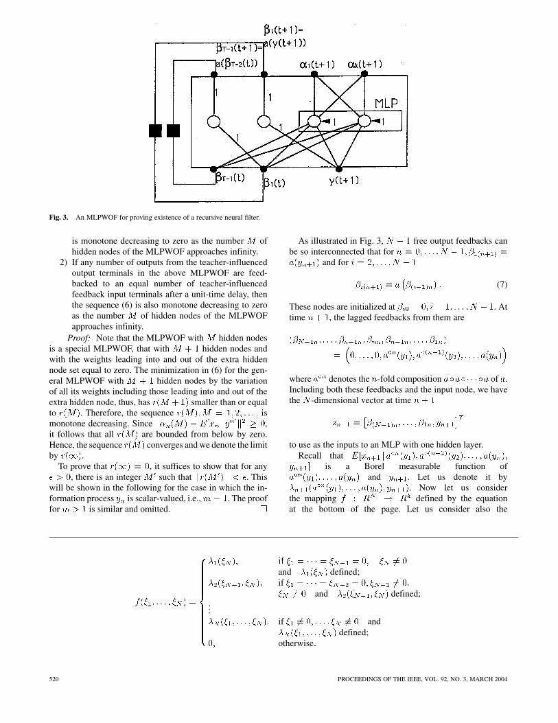
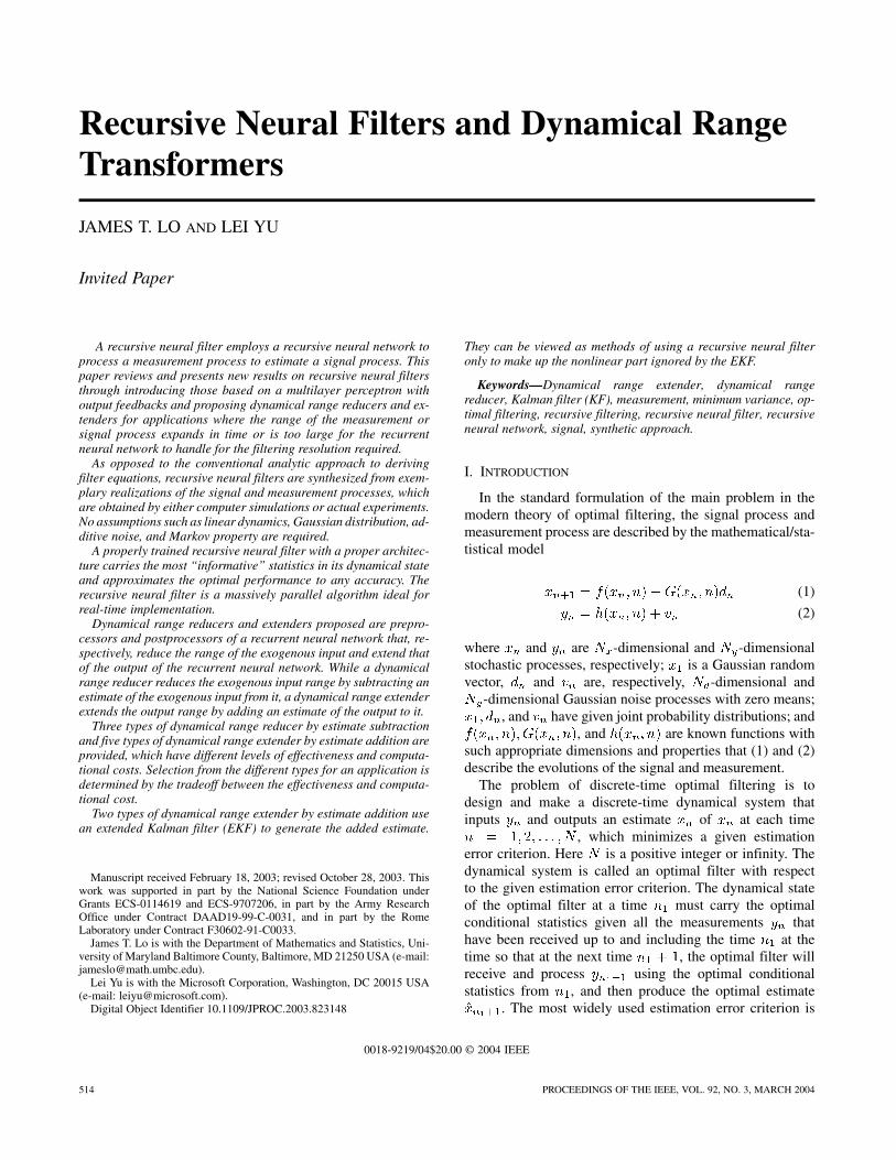
Fig. 3. An MLPWOF for proving existence of a recursive neural filter.

is monotone decreasing to zero as the number ofhidden nodes of the MLPWOF approaches infinity.

2) If any number of outputs from the teacher-influencedoutput terminals in the above MLPWOF are feed-backed to an equal number of teacher-influencedfeedback input terminals after a unit-time delay, thenthe sequence (6) is also monotone decreasing to zeroas the number of hidden nodes of the MLPWOFapproaches infinity.

Proof: Note that the MLPWOF with hidden nodesis a special MLPWOF, that with hidden nodes andwith the weights leading into and out of the extra hiddennode set equal to zero. The minimization in (6) for the gen-eral MLPWOF with hidden nodes by the variationof all its weights including those leading into and out of theextra hidden node, thus, has smaller than or equalto . Therefore, the sequence ismonotone decreasing. Since ,it follows that all are bounded from below by zero.Hence, the sequence converges and we denote the limitby .

To prove that , it suffices to show that for any, there is an integer such that . This

will be shown in the following for the case in which the in-formation process is scalar-valued, i.e., . The prooffor is similar and omitted.

As illustrated in Fig. 3, free output feedbacks canbe so interconnected that for

and for

(7)

These nodes are initialized at . Attime , the lagged feedbacks from them are

where denotes the -fold composition of .Including both these feedbacks and the input node, we havethe -dimensional vector at time

to use as the inputs to an MLP with one hidden layer.Recall that

is a Borel measurable function ofand . Let us denote it by

. Now let us considerthe mapping defined by the equationat the bottom of the page. Let us consider also the

and defined;if

and defined;...

if anddefined;

otherwise


measures defined on the Borel sets in by (denotingby )

if forotherwise;

if forotherwise;

...

Notice that is also a measure on the Borelsets in and that

Since are assumed to have compact ranges,it is easy to see that and all havecompact ranges. Hence, there is a compact set in suchthat .

Consider now the normed space with the normdefined by for each -dimen-sional function . By Corollary 2.2 of thepaper [37] by Hornik et al., the -dimensional functions rep-resented by all the MLPs with output nodes and a singlelayer of hidden nodes are dense in . It then fol-lows that for any , there is such an MLP that the func-tion that it represents satisfies

Let us translate the left side of this inequality fromback to the probability space

where the last equality holds, because the -fields generatedby and are identicaldue to the monotonicity of .

We notice that the foregoing approximation MLP,, and the free output feedbacks (7)

discussed earlier form an MLPWOF with a single hiddenlayer. The number of hidden nodes of this MLPWOF isthe sum of that of the MLP and . Recalling (6), wehave

since minimizes the error function in (6) by the varia-tion of the weights of an MLPWOF with exactly the samearchitecture as for the MLPWOF constructed earlier. Thiscompletes the proof of 1).

The MLPWOF with teacher-influenced feedbacks thatis described in 2) can be viewed as a general case ofthe MLPWOF described in 1): if the weights on thoseteacher-influenced feedback connections of the former areset equal to zero, it is reduced to an MLPWOF withoutthe teacher-influenced feedbacks. Therefore, the sequence

of the MLPWOF with teacher-influenced feedbacksis also monotone decreasing to zero as the number ofhidden nodes of the MLPWOF approaches infinity. Thiscompletes the proof of 2).

As discussed earlier on, free output feedbacks are usedto carry conditional statistics required for optimal filtering.Therefore, the number of free output feedbacks needed de-pends very much on the properties and the probability dis-tributions of the signal and information processes andindividually and jointly. For instance, if and satisfy1) and 2) with and being linear in constant, and

, and Gaussian, the free output feedbacks neededfor minimum variance filtering are the conditional mean andcovariances of given , regardless of .

VI. DYNAMICAL RANGE REDUCERS

A dynamical range reducer is a preprocessor of an RNNthat dynamically transforms at least one component of theexogenous input process such as an information process andsends the resulting process to at least one input terminal ofthe RNN. A possible benefit of using a dynamical range re-ducer is a reduction of the valid input range or approxima-tion capability required of the RNN so as to ease the RNNsize and training data requirements and thereby lessen the


training difficulty. Another possible benefit is an enhance-ment of the generalization capability of the RNN beyond thelength of time for which the training data are available.

A basic scheme for dynamically transforming the th com-ponent of an exogenous input process is to subtractsome estimate of from at every time point . Ascheme that generates a causal estimate is called an aux-iliary estimator of . The resulting difference, , isused at time as the th component of the input vector tothe RNN. A device that comprises an auxilliary estimator togenerate an auxiliary estimate , and a subtractor to per-form the subtraction, , is called a dynamical rangereducer by estimate subtraction.

The purpose of the auxiliary estimate is only to reduce theinput range of the RNN. Therefore, the auxiliary estimatedoes not have to be very accurate. However, notice that thedifference process is causally equiv-alent to the information process only ifis used jointly with the difference process. If a dynamicalrange reducer by estimate subtraction is employed for recur-sive neural filtering, there are three cases to be considered.

Case 1) The initial signal is a fixed vector. In this case,the RNN will learn to integrate this vector intothe estimates produced by the RNN during itstraining.

Case 2) The signal process is observable from the differ-ence process . In this case, theestimate produced by the RNN will still convergeto that of the optimal estimate given the originalinformation process. It only takes a little longer.

Case 3) A good estimate of the initial signal is available.In this case, we use an MLPWOF into whichthe initial signal can be loaded through theteacher-influenced output feedback terminals ofthe MLPWOF. If the estimate of the initial signalis good enough to determine a good estimate ofthe first measurement , the difference processresulting from the dynamical range reducertogether with the initial signal is about causallyequivalent to the information process, and thefiltering performance of the MLPWOF is aboutthe same as that of the optimal filter based on theoriginal information process .

Three types of dynamical range reducer by estimate sub-traction are given as examples in the following:

A. Range Reducers by Differencing

If an information process consists of the vector values,at discrete time points, of a continuous continuous-timeprocess, then the vector value is a “reasonably good”estimate of the vector value . This observation motivateda simple, yet effective way to reduce the range of themeasurements, when two consecutive measurementsand are not too far apart.

Consider the recursive neural filter depicted in Fig. 4. Adifferencer that consists of a unit time delay and a subtractoris concatenated at a input terminal of an RNN. At each timepoint , the differencer subtracts the preceding measurement

Fig. 4. A range reducer by differencing.

Fig. 5. A range reducer by linear prediction.

from the current measurement and feeds the dif-ference to the th input terminal of the RNN.

There are three ways to initialize the differencer. One wayis to start the recursive neural filter at , the th com-ponent of the first input vector to the RNN beingand the first output vector of the RNN being . The secondway is to determine an initialization value for jointly withthe weights and initial dynamical state of the RNN intraining. In the operation of the recursive neural filter, the thcomponent of the first input vector to the RNN is .The third way is to use the best available estimate ofand then use as the th component of the first inputvector to the RNN consistently in the training and operationof the recursive neural filter.

B. Range Reducers by Linear Prediction

Consider the recursive neural filter depicted in Fig. 5,where one dynamical range reducer is shown, which con-sists of a linear predictor, a unit time delay device, and asubtractor.


The linear predictor inputs the th component of the inputprocess to the recursive neural filter, which input process isthe information process , and outputs a predictionof . After a unit time delay, the preceding prediction

is now subtracted from by the subtractor. The resultingdifference is then input to the RNN at its th inputterminal.

A range reducer by differencing is obviously a specialrange reducer by linear prediction, in which the estimate

generated by the linear predictor is simply . Ageneral linear predictor is written as ,where is a fixed positive integer called the order of thelinear predictor, and are the linear predictor coefficients[38]. Realizations of the th component of the informationprocess, which are part of the training data to be discussed inthe sequel, are used to determine so thatthe linear predictor predicts in thestandard least-squares sense. A fast and stable algorithm forthis can be found in [39]. Some other algorithms can be foundin [38].

There are two ways to initialize the linear predictor. Oneway is to start the recursive neural filter at , theth component of the first input vector to the RNN being

and the first output vector of the RNNbeing . The second way is to determine initializationvalues, jointly with the weights

and initial dynamical state of the RNN in training. In theoperation of the recursive neural filter, the th component ofthe first input vector to the RNN is .

C. Range Reducers by Model-Aided Prediction

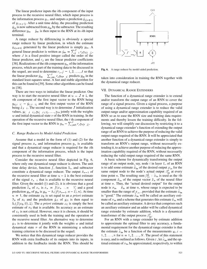
Assume that a model in the form of (1) and (2) for thesignal process and information process is availableand that a dynamical range reducer is required for the thcomponent of the information process, which is the inputprocess to the recursive neural filter.

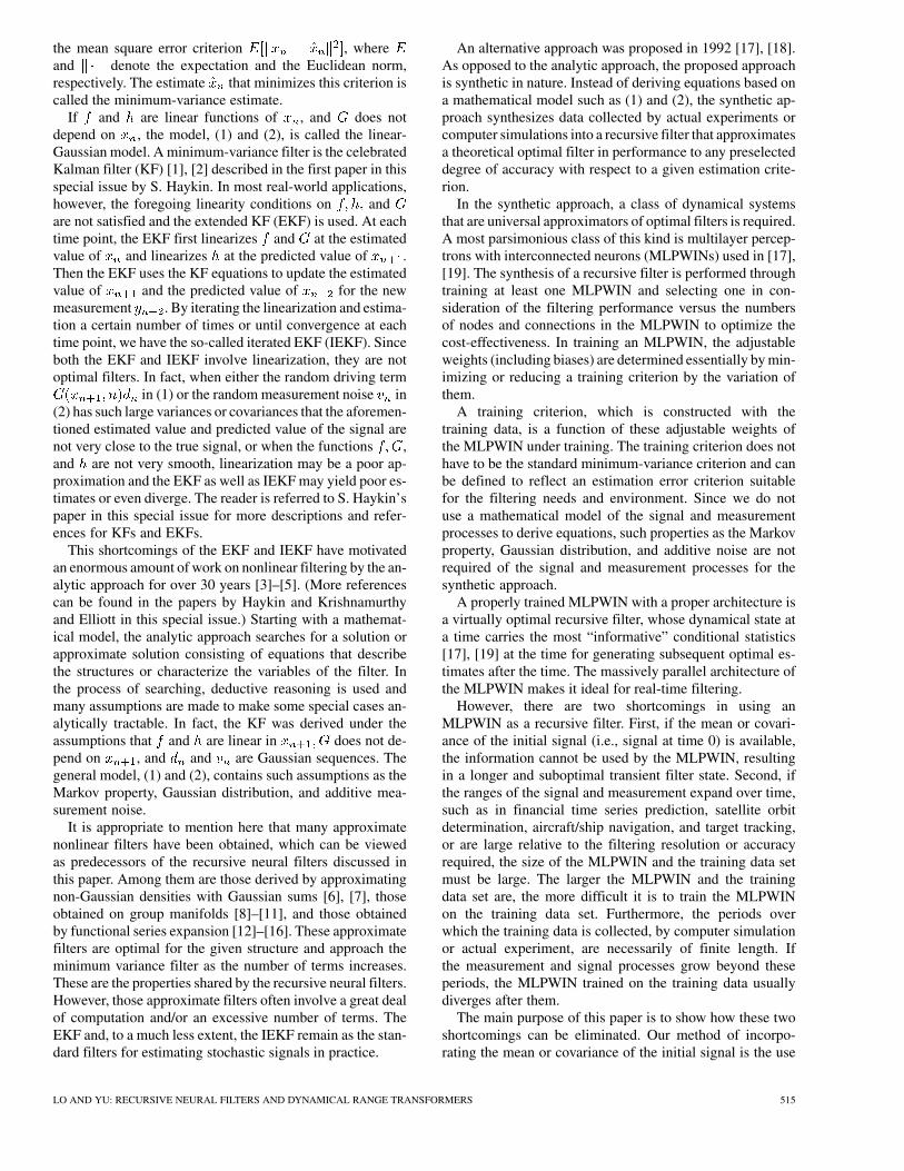
Consider the recursive neural filter depicted in Fig. 6,where only one dynamical range reducer is shown. The unittime delay device, function , function , and subtractorconstitute a dynamical range reducer. The output ofthe recursive neural filter at time is the best estimateof the signal that is available to the recursive neuralfilter. Given the model (1) and (2), it is obvious that a goodprediction of is and a goodprediction of is . At time

, the estimate is set equal to an a priori estimateof and the prediction of is then equal to

. The a priori estimate is simply the bestestimate of that is available. Its accuracy as an estimateof is not critical. However, once it is chosen, it should beconsistently used in both the training and the operation ofthe recursive neural filter. An alternative way to determine

is to determine it jointly with the weights and initialdynamical state of the RNN in minimizing a selectedtraining criterion to be discussed in the sequel.

We notice that this dynamical range reducer provides theRNN with extra feedbacks of its outputs into its inputs, inaddition to the feedbacks inside the RNN. This should be

Fig. 6. A range reducer by model-aided prediction.

taken into consideration in training the RNN together withthe dynamical range reducer.

VII. DYNAMICAL RANGE EXTENDERS

The function of a dynamical range extender is to extendand/or transform the output range of an RNN to cover therange of a signal process. Given a signal process, a purposeof using a dynamical range extender is to reduce the validoutput range and/or approximation capability required of anRNN so as to ease the RNN size and training data require-ments and thereby lessen the training difficulty. In the fol-lowing, we will simplify our discussion by restricting it to adynamical range extender’s function of extending the outputrange of an RNN to achieve the purpose of reducing the validoutput range required of the RNN. It will be appreciated thatanother function of a dynamical range extender is simply totransform an RNN’s output range, without necessarily ex-tending it, to achieve another purpose of reducing the approx-imation capability required of the RNN, without necessarilyreducing the valid output range required of the same RNN.

A basic scheme for dynamically transforming the outputrange of an output node, say, node in layer , of an RNNis to add some estimate of the desired output for thesame output node to the node’s actual output at everytime point . The resulting sum is used as the thcomponent of the output vector of the neural filterat time . Thus, the “actual desired output” for the outputnode is at time , whose range is expected to besmaller than the range of , provided that the estimateis “good.” The estimate will be called an auxiliary esti-mate of and a scheme that generates this estimate willbe called an auxiliary estimator. A device that comprises suchan auxiliary estimator and an adder will be called dynamicalrange extender by estimate addition, which is a dynamicaltransformer of the output process .

For an RNN with a range extender by estimate additionto approximate the optimal filter to any accuracy, a funda-mental requirement for the dynamical range extender is thatthe estimate be a function of the measurements

for . The proof of this statementis easy, and is outlined as follows. Given , let and the op-timal estimate of be approximated, respectively, to within


Fig. 7. A range extender by accumulation.

by two RNNs with respect to the minimum-varianceerror criterion. Then their difference approximatesto within . Since the combination of the two RNNs can beviewed as an RNN, the proof is completed.

Five types of range extender by estimate addition, whoseauxiliary estimators have different levels of estimation accu-racy and different levels of computational cost, are given inthe following.

A. Range Extenders by Accumulation

If a signal process consists of the vector values,at discrete time points, of a slowly varying continuouscontinuous-time process, then the vector value is agood approximate of , and a good estimate of isa “reasonably good” estimate of the vector value . Thisobservation motivated a simple, yet effective way to extendthe output range of an RNN in a neural filter, when twoconsecutive signals and are not too far apart.

Consider the neural filter depicted in Fig. 7. Only one ac-cumulator used as a dynamical range extender is shown. Theaccumulator, consisting of a unit time delay device and anadder, is concatenated directly to output node of the RNN.At each time point , the accumulator adds the output ofthe RNN to the accumulator’s output at the precedingtime point . Thus the accumulator accumulates all theoutputs of output node of the RNN from onward plusthe initial accumulation denoted by . Mathematically, theaccumulator is described simply by

(8)

Here, the RNN actually estimates the difference, which is expected to have a much smaller

range than does , if the two consecutive signals andare not too far apart. If a good a priori estimate is

given of , it should be used as the initial accumulation. Otherwise, the initial accumulation can be deter-

mined together with the weights and/or parameters andthe initial dynamical state of the RNN in minimizing atraining criterion for the neural filter.

Fig. 8. A range extender by Kalman filtering.

Note that is a function of , for. Viewing as an estimate of that

is added to the output of output node , we see that theaccumulator is a range extender by estimate addition, whichsatisfies the fundamental requirement for a range extender byestimate addition as stated earlier on. An accumulator usedas a dynamical range extender will be called a range extenderby accumulation.

B. Range Extenders by Kalman Filtering

Assume that a model in the form of (1) and (2) for thesignal process and measurement process is availableand that a dynamical range extender is required for everyoutput node of the RNN in a neural filter.

Consider the neural filter depicted in Fig. 8, where onlyone dynamical range extender for an output node is shown.Recall a solid square represents a unit time delay device. TheEKF and the adder constitute a dynamical range extender.The EKF uses the output from the neural filter, the errorcovariance matrix from itself, and the measurementvector to produce an estimate of . The RNN is thenemployed only to estimate the difference for the thsignal component. The range of the difference is expected tobe much smaller than , if is a good estimate of .Denoting the th output of the RNN by , the estimateof generated by the neural filter is .

The EKF equations are

(9)

(10)

(11)

(12)

(13)

(14)

where , and. At , we initialize the neural


filter by setting and to activate the aboveEKF equations.

Note that is indeed a function of , for, satisfying the aforementioned fundamental

requirement for a range extender by estimate addition.We stress here that the above EKF equations involve the

outputs of the RNN through and are, thus, not the stan-dard EKF equations. If an RNN is properly selected andtrained, the estimate generated by the above EKF equa-tions is better than the standard extended Kalman estimate.

If the signal process is only a part of the process de-scribed by (1), the estimate generated by the neuralfilter is then only a part of the “preceding estimate” used inthe EKF equations for (1) and (2). The rest of the “precedingestimate” used is necessarily the corresponding componentsof the preceding EKF estimate generated by these EKF equa-tions.

The RNN with range extenders by Kalman filtering canbe viewed as using the RNN to make up the nonlinear partof an optimal estimate that is ignored by the EKF due tolinearization.

C. Range Extenders by Feedforward Kalman Filtering

The only difference between this type of dynamical rangeextender and the preceding type, namely, range extendersby Kalman filtering, is that the “preceding estimate”used in the EKF equations (9)–(14) is now replaced by .Thus, the EKF equations used here are the standard EKFequations without the involvement of generated by anRNN. This type of dynamical range extender requires thatthe EKF does not diverge and is useful for improving ex-isting EKFs.

A range extender by feedforward Kalman filtering isusually inferior to a range extender by Kalman filtering.However, including a range extender by feedforward Kalmanfiltering in a neural system does not incur much extra com-putation for training the recursive neural filter. Since theEKF equations used here do not involve the RNN in theneural system, the only special treatment in training for arange extender by feedforward Kalman filtering is to use

instead ofas the target output process for the output node involvedin the RNN.

D. Range Extenders by Linear Prediction

Consider the recursive neural filter depicted in Fig. 9where only one dynamical range extender is shown. Theone shown is a range extender by estimate addition thatconsists of a linear predictor, a unit time delay device,and an adder, and is concatenated to output node of anRNN. The estimate , to be added to to yield , i.e.,

, is generated by a linear predictor. A rangeextender by accumulation can be viewed as a special case inwhich is used as the predicted value of .

A better estimate of than , which is used ina range extender by accumulation, can be obtained by thelinear predictor , where is a fixedpositive integer called the order of the linear predictor and

are the linear predictor coefficients [38]. However, before

Fig. 9. A range extender by linear prediction.

both the RNN and the linear predictor are fully specified, thesequence is not avail-able, preventing us from applying standard methods to deter-mine the linear predictor coefficients andthereby specify the linear predictor. To get around this diffi-culty, we may determine the linear predictor coefficients forpredicting the signal instead. More specifically, we userealizations of the th component of the signal process,which realizations are part of the training data to be discussedin the sequel, to determine , so that thelinear finite-impulse response (FIR) filterpredicts in the standard least-squares sense. A fast andstable algorithm for this can be found in [38].

Then we use these coefficients as thecoefficients in the linear predictor forpredicting . The resulting linear predictor is expected togenerate good estimate of , provided mimicsclosely.

To initialize the linear predictor at , we need theinitialization values in both thetraining and the operation of the recursive neural filter. If thesignals are available atin the operation of the recursive neural filter in the appli-cation under consideration, we may include realizations of

in the training data set in addi-tion to those of . In training, a realizationof is used as the initializationvalues .

If the signals are not avail-able at time in the operation of the recursive neuralfilter in the application under consideration, we may use astarter-filter to process for estimating

. The resulting estimates are thenused as the initialization values. Here, of course, we need themeasurements , which are either extrameasurements or the measurements with thetime scale shifted. We may employ an EKF as a starter filter.Since is usually small and the ranges of the signal and


information processes cannot be very large over the timeinterval , a simple recursiveneural filter without dynamical range extenders and reducersis expected to work nicely here as a starter filter.

Now holding the coefficients constant, we synthesizethe training data into an RNN. If the resulting recursiveneural filter, including the linear predictor, adder, and RNN,works satisfactorily, the process of designing a recursiveneural filter is completed. Otherwise, we may increaseand repeat the above process of determining and thensynthesizing an RNN again or we may adjust the valuesof together with the weights and theinitial dynamical state of the RNN by minimizing thetraining criterion further, using the existing values of ,and as the initial guess in the minimization process.

E. Range Extenders by Feedforward Linear Estimation

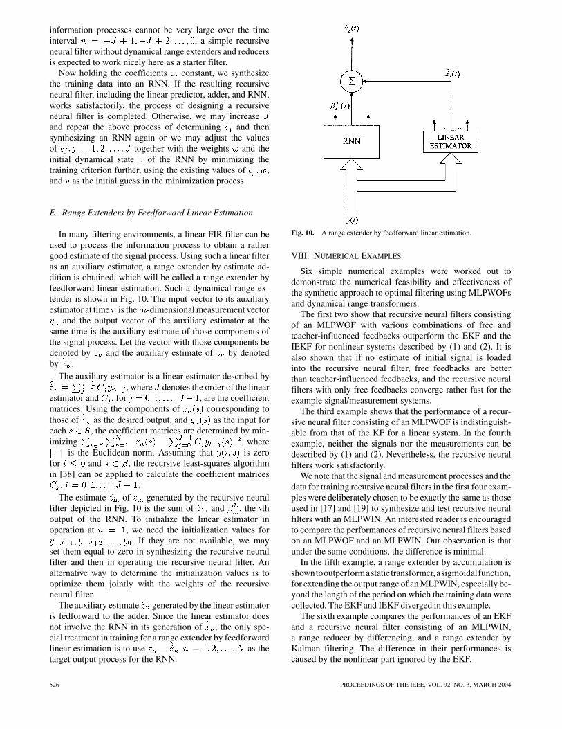
In many filtering environments, a linear FIR filter can beused to process the information process to obtain a rathergood estimate of the signal process. Using such a linear filteras an auxiliary estimator, a range extender by estimate ad-dition is obtained, which will be called a range extender byfeedforward linear estimation. Such a dynamical range ex-tender is shown in Fig. 10. The input vector to its auxiliaryestimator at time is the -dimensional measurement vector

and the output vector of the auxiliary estimator at thesame time is the auxiliary estimate of those components ofthe signal process. Let the vector with those components bedenoted by and the auxiliary estimate of by denotedby .

The auxiliary estimator is a linear estimator described by, where denotes the order of the linear

estimator and , for , are the coefficientmatrices. Using the components of corresponding tothose of as the desired output, and as the input foreach , the coefficient matrices are determined by min-imizing , where

is the Euclidean norm. Assuming that is zerofor and , the recursive least-squares algorithmin [38] can be applied to calculate the coefficient matrices

.The estimate of generated by the recursive neural

filter depicted in Fig. 10 is the sum of and , the thoutput of the RNN. To initialize the linear estimator inoperation at , we need the initialization values for

. If they are not available, we mayset them equal to zero in synthesizing the recursive neuralfilter and then in operating the recursive neural filter. Analternative way to determine the initialization values is tooptimize them jointly with the weights of the recursiveneural filter.

The auxiliary estimate generated by the linear estimatoris fedforward to the adder. Since the linear estimator doesnot involve the RNN in its generation of , the only spe-cial treatment in training for a range extender by feedforwardlinear estimation is to use as thetarget output process for the RNN.

Fig. 10. A range extender by feedforward linear estimation.

VIII. NUMERICAL EXAMPLES

Six simple numerical examples were worked out todemonstrate the numerical feasibility and effectiveness ofthe synthetic approach to optimal filtering using MLPWOFsand dynamical range transformers.

The first two show that recursive neural filters consistingof an MLPWOF with various combinations of free andteacher-influenced feedbacks outperform the EKF and theIEKF for nonlinear systems described by (1) and (2). It isalso shown that if no estimate of initial signal is loadedinto the recursive neural filter, free feedbacks are betterthan teacher-influenced feedbacks, and the recursive neuralfilters with only free feedbacks converge rather fast for theexample signal/measurement systems.

The third example shows that the performance of a recur-sive neural filter consisting of an MLPWOF is indistinguish-able from that of the KF for a linear system. In the fourthexample, neither the signals nor the measurements can bedescribed by (1) and (2). Nevertheless, the recursive neuralfilters work satisfactorily.

We note that the signal and measurement processes and thedata for training recursive neural filters in the first four exam-ples were deliberately chosen to be exactly the same as thoseused in [17] and [19] to synthesize and test recursive neuralfilters with an MLPWIN. An interested reader is encouragedto compare the performances of recursive neural filters basedon an MLPWOF and an MLPWIN. Our observation is thatunder the same conditions, the difference is minimal.

In the fifth example, a range extender by accumulation isshowntooutperformastatictransformer,asigmoidalfunction,for extending the output range of an MLPWIN, especially be-yond the length of the period on which the training data werecollected. The EKF and IEKF diverged in this example.

The sixth example compares the performances of an EKFand a recursive neural filter consisting of an MLPWIN,a range reducer by differencing, and a range extender byKalman filtering. The difference in their performances iscaused by the nonlinear part ignored by the EKF.


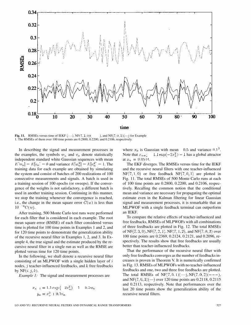
Fig. 11. RMSEs versus time of IEKF (� � �); NF(7; 1; 0)(��), and NF(7;0; 1)(—) for Example1. The RMSEs of them over 100 time points are 0.2800, 0.2200, and 0.2106, respectively.

In describing the signal and measurement processes inthe examples, the symbols and denote statisticallyindependent standard white Gaussian sequences with mean

and variance . Thetraining data for each example are obtained by simulatingthe system and consist of batches of 200 realizations of 100consecutive measurements and signals. A batch is used ina training session of 100 epochs (or sweeps). If the conver-gence of the weights is not satisfactory, a different batch isused in another training session. Continuing in this manner,we stop the training whenever the convergence is reached,i.e., the change in the mean square error is less than

.After training, 500 Monte Carlo test runs were performed

for each filter that is considered in each example. The rootmean square error (RMSE) of each filter considered versustime is plotted for 100 time points in Examples 1 and 2, andfor 120 time points to demonstrate the generalization abilityof the recursive neural filter in Examples 1, 2, and 3. In Ex-ample 4, the true signal and the estimate produced by the re-cursive neural filter in a single run as well as the RMSE areplotted versus time for 120 time points.

In the following, we shall denote a recursive neural filterconsisting of an MLPWOF with a single hidden layer ofnodes, teacher-influenced feedbacks, and free feedbacksby NF .

Example 1: The signal and measurement processes are

where is Gaussian with mean and variance .Note that has a global attractorat .

The EKF diverges. The RMSEs versus time for the IEKFand the recursive neural filters with one teacher-influencedNF or free feedback NF are plotted inFig. 11. The total RMSEs of 500 Monte Carlo runs at eachof 100 time points are 0.2800, 0.2200, and 0.2106, respec-tively. Recalling the common notion that the conditionalmean and variance are necessary for propagating the optimalestimate even in the Kalman filtering for linear Gaussiansignal and measurement processes, it is remarkable that anMLPWOF with a single feedback terminal can outperforman IEKF.

To compare the relative effects of teacher-influenced andfree feedbacks, RMSEs of MLPWOFs with all combinationsof three feedbacks are plotted in Fig. 12. The total RMSEsof NF NF NF , and NF over100 time points are 0.2369, 0.2124, 0.2121, and 0.2096, re-spectively. The results show that free feedbacks are usuallybetter than teacher-influenced feedbacks.

That the performance of the recursive neural filter withonly free feedbacks converges as the number of feedbacks in-creases is proven in Theorem V. It is numerically confirmedin Fig. 13. RMSEs of MLPWOFs with no teacher-influencedfeedbacks and one, two and three free feedbacks are plotted.The total RMSEs of NF NF ,and NF — over 120 time points are 0.2118, 0.2115and 0.2113, respectively. Note that performances over thelast 20 time points show the generalization ability of therecursive neural filters.


Fig. 12. RMSEs versus time of NF(7; 3; 0)(� � �); NF(7;2; 1) (� � �); NF(7;1; 2) (��),and NF(7;0; 3) (—) for Example 1. The RMSEs of them over 100 time points are 0.2369,0.2124, 0.2121, and 0.2096, respectively.

Fig. 13. RMSEs versus time of NF(7;0; 1) (� � �); NF(7;0; 2) (��), and NF(7;0; 3) (—) forExample 1. The RMSEs of them over 120 time points are 0.2118, 0.2115, and 0.2113, respectively.

Example 2: The signal and measurement processes are where is Gaussian with mean zero and variance . Notethat is a chaotic process.

The RMSEs versus time for the EKF, IEKF, and recur-sive neural filters with one teacher-influenced NF orfree feedback NF are plotted in Fig. 14. The total


Fig. 14. RMSEs versus time of EKF (� � �); IEKF(� � �); NF(7; 1; 0) (��), andNF(7;0; 1) (—) for Example 2. The RMSEs of them over 100 time points are 0.3371, 0.2807,0.1942, and 0.1801, respectively.

RMSEs over 100 time points are 0.3371, 0.2807, 0.1942, and0.1801, respectively. Recalling the common notion that theconditional mean and variance are necessary for propagatingthe optimal estimate even in the Kalman filtering for linearGaussian signal and measurement processes, it is remarkablethat an MLPWOF with a single feedback terminal can out-perform an EKF and IEKF.

To compare the relative effects of teacher-influenced andfree feedbacks, RMSEs of MLPWOFs with all combinationsof three feedbacks are plotted in Fig. 15. The total RMSEsof NF NF NF , and NF over100 time points are 0.1836, 0.1833, 0.1774, and 0.1764, re-spectively. The results show that free feedbacks are betterthan teacher-influenced feedbacks.

That the performance of the recursive neural filter withonly free feedbacks converges as the number of feedbacksincreases is proven in Theorem V. It is numerically confirmedin Fig. 16. RMSEs of MLPWOFs with no teacher-influencedfeedbacks and one, two, and three free feedbacks are plotted.The total RMSEs of NF NF ,and NF — over 120 time points are 0.1786, 0.1767,and 0.1763, respectively. Note that performances over the last20 time points show the generalization ability of the recursiveneural filters.


where is Gaussian with mean zero and variance .

The RMSEs versus time for the KF and NF areshown in Fig. 17. We note that the two lines are virtually thesame.


where is Gaussian with mean zero and variance . Notethat neither the signal nor the measurement process can betransformed into (1) or (2). The EKF and IEKF do not applyhere.

The true signal and its estimates produced by theNF in a single run are shown in Fig. 18. The recur-sive neural filter tracks the true signal well except at a fewtime points, and is able to generalize beyond the time lengthof training data, 100.

The RMSEs versus time for the NF NF ,and NF are plotted in Fig. 19, which show that theperformance of the recursive neural filter with only free feed-backs converges as the number of feedbacks increases. Thisconfirms Theorem V.


(15)

(16)

where and are independent standard white Gaussiansequences, and . The measurements are confined


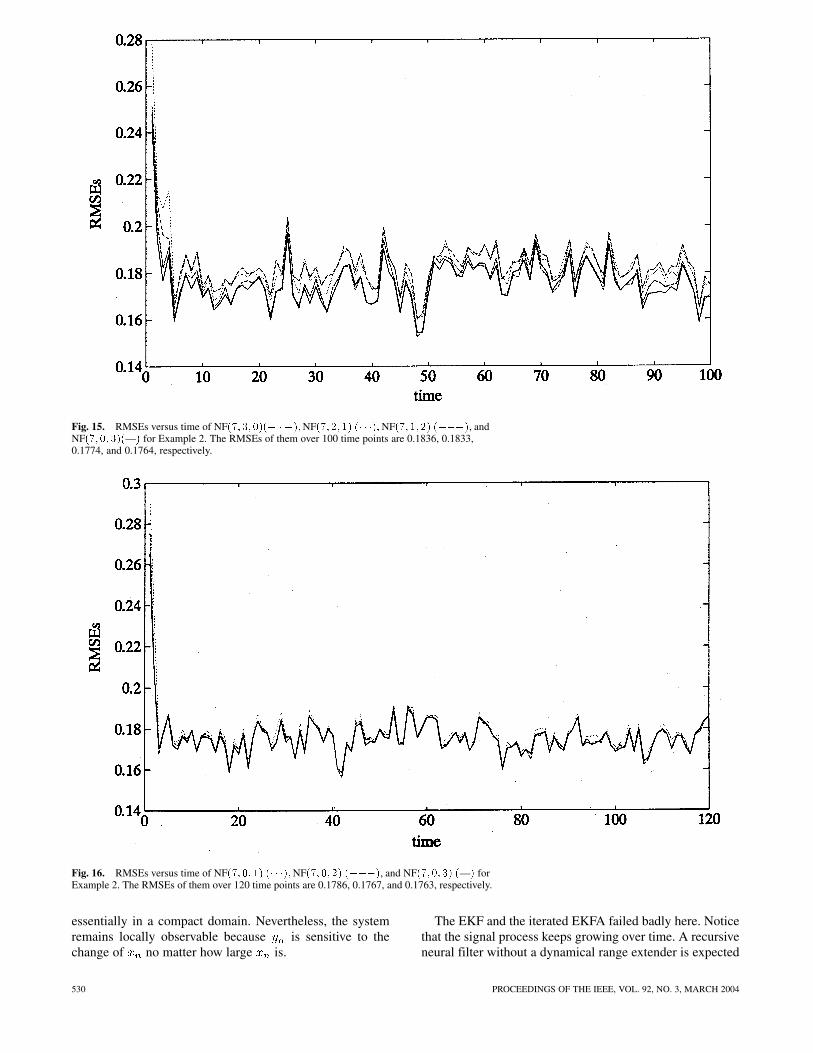
Fig. 15. RMSEs versus time of NF(7; 3; 0)(� � �); NF(7;2; 1) (� � �); NF(7;1; 2) (��), andNF(7;0; 3)(—) for Example 2. The RMSEs of them over 100 time points are 0.1836, 0.1833,0.1774, and 0.1764, respectively.

Fig. 16. RMSEs versus time of NF(7;0; 1) (� � �); NF(7;0; 2) (��), and NF(7;0; 3) (—) forExample 2. The RMSEs of them over 120 time points are 0.1786, 0.1767, and 0.1763, respectively.

essentially in a compact domain. Nevertheless, the systemremains locally observable because is sensitive to thechange of no matter how large is.

The EKF and the iterated EKFA failed badly here. Noticethat the signal process keeps growing over time. A recursiveneural filter without a dynamical range extender is expected


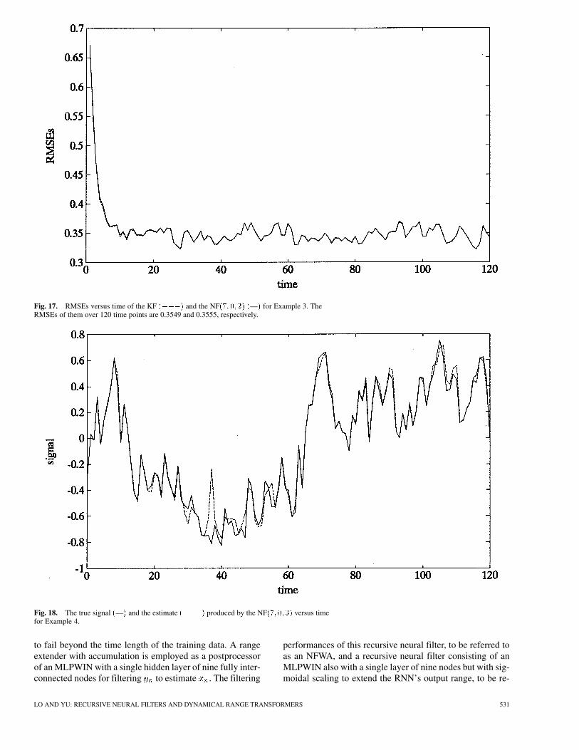
Fig. 17. RMSEs versus time of the KF (��) and the NF(7; 0; 2) (—) for Example 3. TheRMSEs of them over 120 time points are 0.3549 and 0.3555, respectively.

Fig. 18. The true signal (—) and the estimate (��) produced by the NF(7;0; 3) versus timefor Example 4.

to fail beyond the time length of the training data. A rangeextender with accumulation is employed as a postprocessorof an MLPWIN with a single hidden layer of nine fully inter-connected nodes for filtering to estimate . The filtering

performances of this recursive neural filter, to be referred toas an NFWA, and a recursive neural filter consisting of anMLPWIN also with a single layer of nine nodes but with sig-moidal scaling to extend the RNN’s output range, to be re-


Fig. 19. RMSEs versus time of NF(7; 0; 1) (� � �); NF(7;0; 2) (��), and NF(7;0; 3) (—) forExample 4. The RMSEs of them over 120 time points are 0.0568, 0.0567, and 0.0565, respectively.

Fig. 20. RMSEs versus time of NFWA (—) and NF(��) for Example 5.

ferred to as an NF, were compared. The RMSEs averagedover 500 runs of the NFWA — and the NF areplotted versus time in Fig. 20. The length of each trainingdata sequence is 100. The recursive neural filters were tested

for 150 time points to assess their ability to generalize. TheNFWA has a better performance than the NF, before 100 timepoints. After 100 time points, the latter deteriorates rapidlywhile the former remains good.


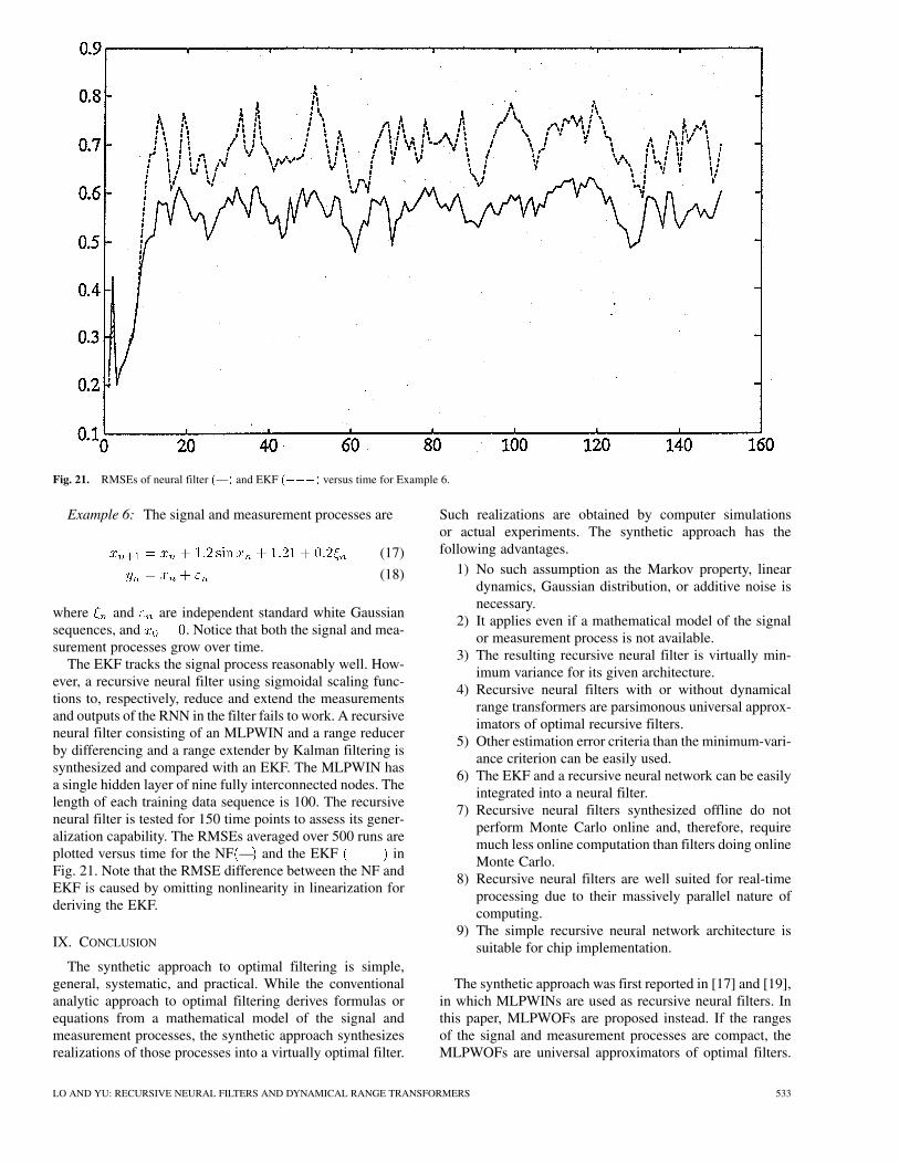
Fig. 21. RMSEs of neural filter (—) and EKF (��) versus time for Example 6.


(17)

(18)

where and are independent standard white Gaussiansequences, and . Notice that both the signal and mea-surement processes grow over time.

The EKF tracks the signal process reasonably well. How-ever, a recursive neural filter using sigmoidal scaling func-tions to, respectively, reduce and extend the measurementsand outputs of the RNN in the filter fails to work. A recursiveneural filter consisting of an MLPWIN and a range reducerby differencing and a range extender by Kalman filtering issynthesized and compared with an EKF. The MLPWIN hasa single hidden layer of nine fully interconnected nodes. Thelength of each training data sequence is 100. The recursiveneural filter is tested for 150 time points to assess its gener-alization capability. The RMSEs averaged over 500 runs areplotted versus time for the NF — and the EKF inFig. 21. Note that the RMSE difference between the NF andEKF is caused by omitting nonlinearity in linearization forderiving the EKF.

IX. CONCLUSION

The synthetic approach to optimal filtering is simple,general, systematic, and practical. While the conventionalanalytic approach to optimal filtering derives formulas orequations from a mathematical model of the signal andmeasurement processes, the synthetic approach synthesizesrealizations of those processes into a virtually optimal filter.

Such realizations are obtained by computer simulationsor actual experiments. The synthetic approach has thefollowing advantages.

1) No such assumption as the Markov property, lineardynamics, Gaussian distribution, or additive noise isnecessary.

2) It applies even if a mathematical model of the signalor measurement process is not available.

3) The resulting recursive neural filter is virtually min-imum variance for its given architecture.

4) Recursive neural filters with or without dynamicalrange transformers are parsimonous universal approx-imators of optimal recursive filters.

5) Other estimation error criteria than the minimum-vari-ance criterion can be easily used.

6) The EKF and a recursive neural network can be easilyintegrated into a neural filter.

7) Recursive neural filters synthesized offline do notperform Monte Carlo online and, therefore, requiremuch less online computation than filters doing onlineMonte Carlo.

8) Recursive neural filters are well suited for real-timeprocessing due to their massively parallel nature ofcomputing.

9) The simple recursive neural network architecture issuitable for chip implementation.

The synthetic approach was first reported in [17] and [19],in which MLPWINs are used as recursive neural filters. Inthis paper, MLPWOFs are proposed instead. If the rangesof the signal and measurement processes are compact, theMLPWOFs are universal approximators of optimal filters.


An MLPWOF used as a recursive neural filter allows us toload an estimate of the initial signal into it, improving thetransient state and hastening the convergence of the filter.

If the range of the signal or measurement process expandsin time or is very large relative to the resolution or accuracy ofthe filtering required, dynamical range reducers or extenders,respectively, are proposed in this paper. Dynamical range re-ducers and extenders have the following advantages.

1) They, respectively, reduce the input and output rangerequired of an RNN.

2) They reduce the amount of training data required.3) They reduce the RNN size and training difficulty for a

given filtering resolution or accuracy.4) They improve the generalization ability of the recur-

sive neural filter, especially beyond the length of theperiod over which the training data are collected.

If a dynamical range reducer is needed and the signal isnonobservable from the outputs of the dynamical range re-ducer, loading an estimate of the initial signal into a recursiveneural filter can overcome this nonobservability problem. Inthis case, an MLPWOF is needed.

Consider using an MLPWIN and an MLPWOF both witha single hidden layer of nodes for optimal filtering for thesame signal and measurement processes. To determine thearchitecture of the latter, we need to determine the numberof nodes in the hidden layer and the number of free feed-backs. On the other hand, to determine the architecture of theformer, we need to determine only the number of nodes in thehidden layer. This is certainly an advantage in synthesizinga filter. However, an estimate of the initial signal cannot beloaded into an MLPWIN. Therefore, an MLPWIN with itsoutputs, which are all teacher-influenced, feedbacked after aunit-time delay to the input layer may be a more desirablearchitecture than that of an MLPWIN or MLPWOF. In suchan RNN with teacher-influenced feedbacks, only the numberof nodes in the single hidden layer needs to be determined,and an estimate of the initial signal can be loaded into theRNN. Such RNNs are obviously universal approximators ofthe optimal filters if the ranges of the signal and measure-ment processes are compact. Numerical examples showingthe numerical feasibility of such RNNs as recursive neuralfilters will soon be reported.

The development of the method of global minimizationthrough convexification [20]–[22] has greatly alleviated thelocal-minimum problem in training neural networks, whichis the main difficulty in the synthetic approach.

REFERENCES

[1] R. E. Kalman, “A new approach to linear filtering and predictionproblems,” J. Basic Eng. Trans. ASME, vol. D82-1, pp. 35–45, 1960.

[2] R. E. Kalman and R. S. Bucy, “New results in linear filtering and pre-diction theory,” J. Basic Eng. Trans. ASME, vol. D83-3, pp. 95–108,1961.

[3] R. S. Liptser and A. N. Shiryayev, Statistics of Random Processes I:General Theory. New York: Springer-Verlag, 1977.

[4] R. S. Bucy and P. D. Joseph, Filtering for Stochastic Processes withApplications to Guidanc, 2nd ed. New York: Chelsea, 1987.

[5] G. Kallianpur and R. L. Karandikar, White Noise Theory of Pre-diction, Filtering, and Smoothing. New York: Gordon & Breach,1988.

[6] J. T. Lo, “Finite dimensional sensor orbits and optimal nonlinear fil-tering,” Ph.D. dissertation, Univ. Southern California, Los Angeles,1969.

[7] , “Finite dimensional sensor orbits and optimal nonlinear fil-tering,” IEEE Trans. Inform. Theory, vol. IT-18, pp. 583–588, Sept.1972.

[8] , “Exponential Fourier densities and estimation and detectionon a circle,” IEEE Trans. Inform. Theory, vol. IT-23, pp. 110–116,Jan. 1977.

[9] J. T. Lo and L. R. Eshleman, “Exponential fourier densities on s andoptimal estimation and detection for directional processes,” IEEETrans. Inform. Theory, vol. IT-23, pp. 321–336, May 1977.

[10] , “Exponential Fourier densities on S0(3) and optimal estima-tion and detection for rotational processes,” SIAM J. Appl. Math.,vol. 36, no. 1, pp. 73–82, Feb. 1979.

[11] , “Exponential Fourier densities and optimal estimation foraxial processes,” IEEE Trans. Inform. Theory, vol. IT-25, pp.463–470, July 1979.

[12] S. K. Mitter and D. Ocone, “Multiple integral expansions for non-linear filtering,” presented at the 18th IEEE Conf. Decision and Con-trol, Ft. Lauderdale, FL, 1979.

[13] J. T. Lo and S. K. Ng, “Optimal orthogonal expansion for estimtion I:Signal in white Gaussian noise,” in Nonlinear Stochastic Problems,R. S. Bucy, J. M. F. Moura, and D. Reidel, Eds. Dordrecht, TheNetherlands, 1983, pp. 291–310.

[14] J. T. Lo and S.-K. Ng, “Optimal Fourier-hermite expansion for esti-mation,” Stoch. Process. Appl., vol. 21, pp. 291–304, 1986.

[15] J. T. Lo, “Optimal estimation for the satellite attitude using startracker measurements,” Automatica, vol. 22, pp. 477–482, 1986.

[16] J. T. Lo and S.-K. Ng, “Optimal functional expansion for estima-tion from counting observations,” IEEE Trans. Inform. Theory, vol.IT-33, pp. 21–35, Jan. 1987.

[17] J. T. Lo, “Synthetic approach to optimal filtering,” in Proc. 1992 Int.Simulation Technology Conf. and 1992 Workshop Neural Networks,pp. 475–481.

[18] , “Optimal filtering by recurrent neural networks,” presented atthe 30th Annu. Allerton Conf. Communication, Control and Com-puting, Monticello, IL, 1992.

[19] , “Synthetic approach to optimal filtering,” IEEE Trans. NeuralNetworks, vol. 5, pp. 803–811, Sept. 1994.

[20] , “Minimization through convexitization in training neural net-works,” in Proc. 2002 Int. Joint Conf. Neural Networks, 2002, pp.1558–1563.

[21] J. T. Lo and D. Bassu, “Robust identification of dynamic systemsby neurocomputing,” presented at the 2001 Int. Joint Conf. NeuralNetworks, Washington, DC.

[22] , “An adaptive method of training multilayer perceptrons,” pre-sented at the 2001 Int. Joint Conf. Neural Networks, Washington,D.C..

[23] J. T. Lo and L. Yu, “Overcoming recurrent neural networks’compactness limitation for neurofiltering,” in Proc. 1997 Int. Conf.Neural Networks, pp. 2181–2186.

[24] J. T. Lo, “Neural network approach to optimal filtering,” RomeLab., Air Force Material Command, Rome, NY, Tech. Rep.RL-TR-94 197, 1994.

[25] T. Parisini and R. Zoppoli, “Neural networks for nonlinear state esti-mation,” Int. J. Robust Nonlinear Control, vol. 4, pp. 231–248, 1994.

[26] A. Alessandri, M. Baglietto, T. Parisini, and R. Zoppoli, “A neuralstate estimator with bounded errors for nonlinear systems,” IEEETrans. Automat. Contr., vol. 44, pp. 2028–2042, Nov. 1999.

[27] A. Alessandri, T. Parisini, and R. Zoppoli, “Neural approximatorsfor nonlinear finite-memory state estimation,” Int. J. Control, vol.67, pp. 275–301, 1997.

[28] T. Parisini, A. Alessandri, M. Maggiore, and R. Zoppoli, “On con-vergence of neural approximate nonlinear state estimators,” in Proc.1997 Amer. Conf. Control, vol. 3, pp. 1819–1822.

[29] S. C. Stubberud, R. N. Lobbia, and M. Owen, “An adaptive extendedKalman filter using artificial neural networks,” in Proc. 34th IEEEConf. Decision and Control, 1995, pp. 1852–1856.

[30] , “Targeted on-line modeling for an extended Kalman filterusing artificial neural networks,” in Proc. 1998 IEEE Int. JointConf. Neural Networks, vol. 2, pp. 1019–1023.


[31] A. G. Parlos, S. K. Menon, and A. F. Atiya, “An algorithmic ap-proach to adaptive state filtering using recurrent neural networks,”IEEE Trans. Neural Networks, vol. 12, pp. 1411–1432, Nov. 2001.

[32] S. Elanayar and Y. C. Shi, “Radial basis function neural networksfor approximation and estimation of nonlinear stochastic dynamicsystems,” IEEE Trans. Neural Networks, vol. 5, pp. 594–603, July1994.

[33] S. Haykin, P. Yee, and E. Derbez, “Optimum nonlinear filtering,”IEEE Trans. Signal Processing, vol. 45, pp. 2774–2786, Nov. 1997.

[34] A. Doucet, N. de Freitas, and N. Gordon, Sequential Monte CarloMethods in Practice. New York: Springer-Verlag, 2001.

[35] S. J. Julier, J. K. Uhlmann, and H. F. Durrant-Whyte, “A new ap-proach for the nonlinear transformation of means and covariancesin filters and estimators,” IEEE Trans. Automat. Contr., vol. 45, pp.477–482, Mar. 2000.

[36] S. J. Julier and J. K. Uhlmann, “Data fusion in nonlinear systems,” inHandbook of Data Fusion, D. Hall and J. Llinas, Eds. Boca Raton,FL: CRC, 2001, ch. 3.

[37] K. Hornik, M. Stinchcombe, and H. White, “Multilayer feedforwardnetworks are universal approximators,” Neural Netw., vol. 2, pp.359–366, 1989.

[38] S. Haykin, Adaptive Filter Theory, 3rd ed. Englewood Cliffs, NJ:Prentice-Hall, 1996.

[39] D. T. M. Slock and T. Kailath, “Numerically stable fast transversalfilters for recursive least squares adaptive filtering,” IEEE Trans.Signal Processing, vol. 39, pp. 92–114, Jan. 1991.

James T. Lo received the B.A. degree inmechanical engineering from National TaiwanUniversity, Taipei, R.O.C., and the Ph.D. degreein aerospace engineering from the University ofSouthern California, Los Angeles.

He was a Postdoctoral Research Associateat Stanford University, Stanford, CA, and atHarvard University, Cambridge, MA. He iscurrently a Professor in the Department ofMathematics and Statistics at University ofMaryland Baltimore County, Baltimore. His

research interests have included optimal filtering, signal processing, andneural computing. In 1992, he published a synthetic approach to optimalfiltering using recurrent neural networks and obtained a best paper awardfor it. The approach is the first practical solution of the long-standingoptimal nonlinear filtering problem in a most general setting. The recursiveneural filter has been proven to approximate the optimal nonlinear filterin performance to any accuracy. In recent years, he has developed generaland systematic methodologies for adaptive, accommodative, and/or robustprocessing, their applications to active noise/vibration control, an effectiveconvexification method of overcoming the local-minimum problem intraining neural networks and estimating nonlinear regression models, and anovel approach to pattern classification and data compression.

Lei Yu received the B.S. degree in geophysicsfrom the Chinese University of Science andTechnology, Hefei, China, in 1987 and the Ph.D.degree in physics from University of Maryland,College Park, in 1992.

He was a Senior Research Scientist at theMaryland Technology Corporation. He iscurrently a Senior Consultant at Microsoft Cor-poration, Washington, DC. His research interestsinclude neural networks and signal processing.


recursive neural filters and dynamical range transformers

Documents