recursive conditioning adnan darwiche computer science department ucla
TRANSCRIPT
Recursive Conditioning
Adnan DarwicheComputer Science Department
UCLA
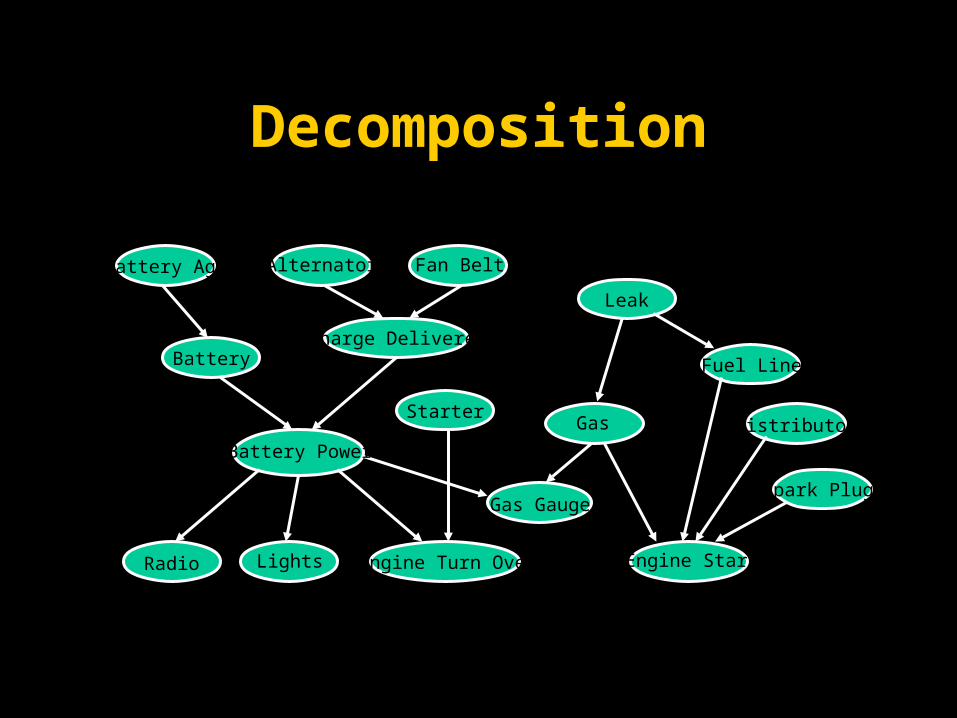
Decomposition
Battery Age Alternator Fan Belt
BatteryCharge Delivered
Battery Power
Starter
Radio Lights Engine Turn Over
Gas Gauge
Gas
Leak
Fuel Line
Distributor
Spark Plugs
Engine Start
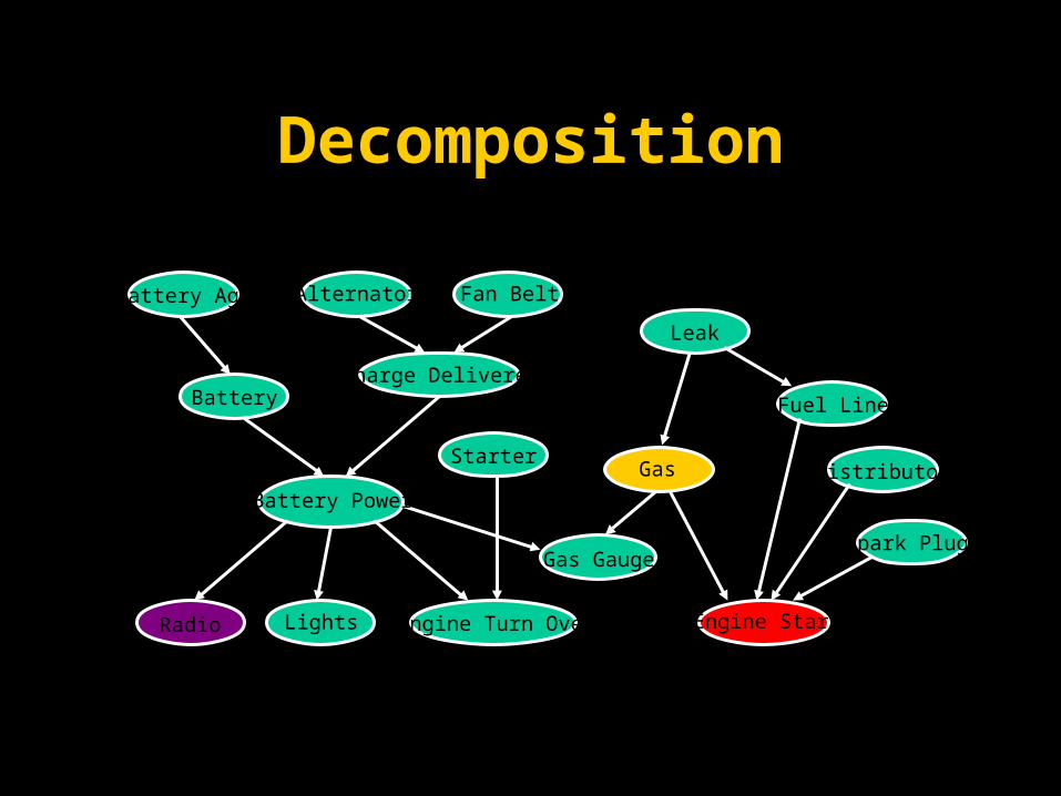
Decomposition
Battery Age Alternator Fan Belt
BatteryCharge Delivered
Battery Power
Starter
Radio Lights Engine Turn Over
Gas Gauge
Gas
Leak
Fuel Line
Distributor
Spark Plugs
Engine Start

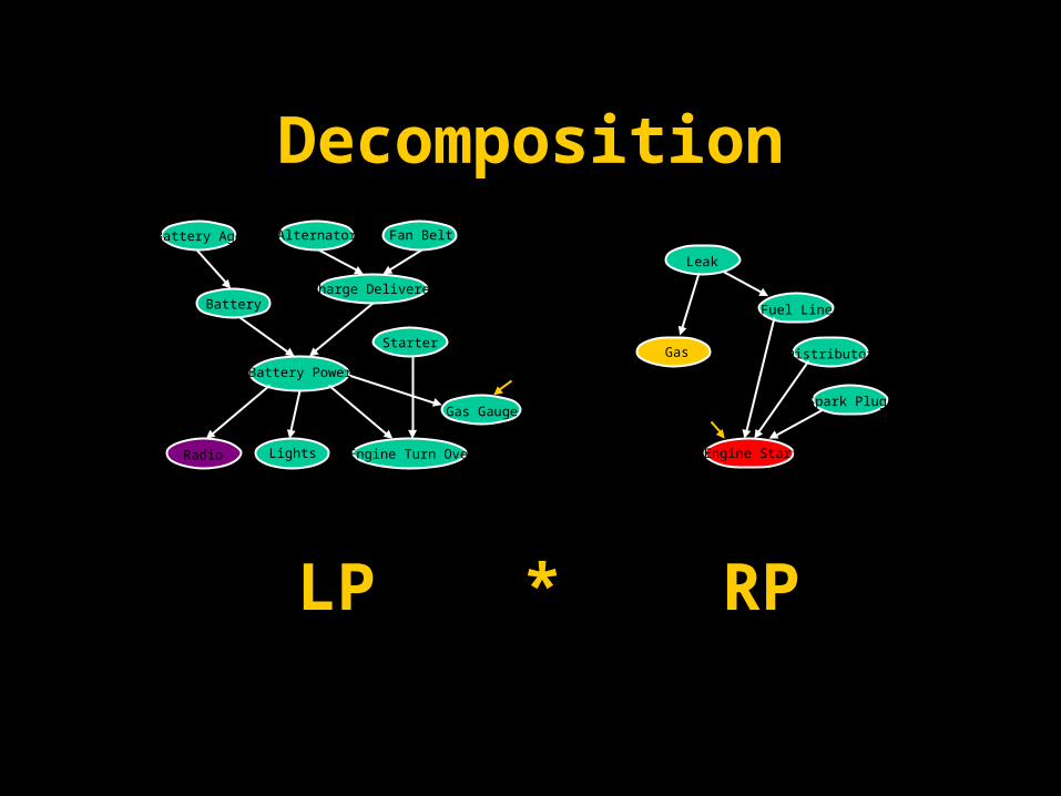
Decomposition
Battery Age Alternator Fan Belt
BatteryCharge Delivered
Battery Power
Starter
Radio Lights Engine Turn Over
Gas Gauge
Gas
Leak
Fuel Line
Distributor
Spark Plugs
Engine Start
DecompositionBattery Age Alternator Fan Belt
BatteryCharge Delivered
Battery Power
Starter
Radio Lights Engine Turn Over
Gas Gauge
Gas
Leak
Fuel Line
Distributor
Spark Plugs
Engine Start
LP RP*

DecompositionBattery Age Alternator Fan Belt
BatteryCharge Delivered
Battery Power
Starter
Radio Lights Engine Turn Over
Gas Gauge
Gas
Leak
Fuel Line
Distributor
Spark Plugs
Engine Start
LP RP*
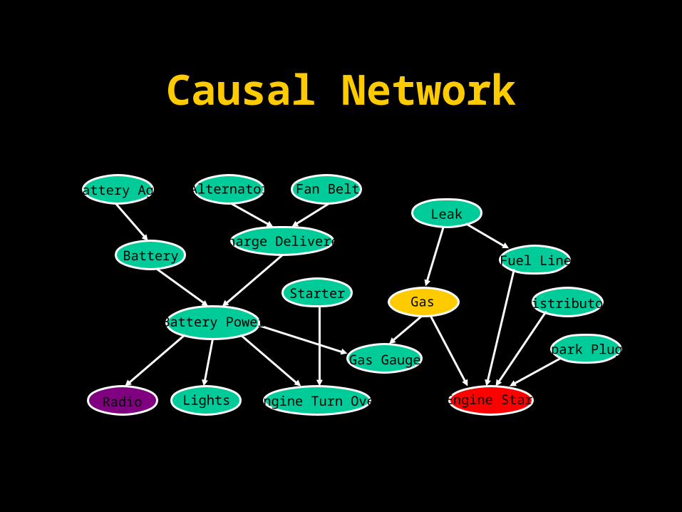
Causal Network
Battery Age Alternator Fan Belt
BatteryCharge Delivered
Battery Power
Starter
Radio Lights Engine Turn Over
Gas Gauge
Gas
Leak
Fuel Line
Distributor
Spark Plugs
Engine Start

Causal Network
Battery Age Alternator Fan Belt
BatteryCharge Delivered
Battery Power
Starter
Radio Lights Engine Turn Over
Gas Gauge
Gas
Leak
Fuel Line
Distributor
Spark Plugs
Engine Start

Case AnalysisBattery Age Alternator Fan Belt
Battery
Charge Delivered
Battery Power
Starter
Radio Lights Engine Turn Over
Gas Gauge
Gas
Leak
Fuel Line
Distributor
Spark Plugs
Engine Start
Case I
Battery Age Alternator Fan Belt
Battery
Charge Delivered
Battery Power
Starter
Radio Lights Engine Turn Over
Gas Gauge
Gas
Leak
Fuel Line
Distributor
Spark Plugs
Engine Start
Case II

Case AnalysisBattery Age Alternator Fan Belt
Battery
Charge Delivered
Battery Power
Starter
Radio Lights Engine Turn Over
Gas Gauge
Gas
Leak
Fuel Line
Distributor
Spark Plugs
Engine Start
Battery Age Alternator Fan Belt
Battery
Charge Delivered
Battery Power
Starter
Radio Lights Engine Turn Over
Gas Gauge
Gas
Leak
Fuel Line
Distributor
Spark Plugs
Engine Start
Case I Case II
LP * RP

Case AnalysisBattery Age Alternator Fan Belt
Battery
Charge Delivered
Battery Power
Starter
Radio Lights Engine Turn Over
Gas Gauge
Gas
Leak
Fuel Line
Distributor
Spark Plugs
Engine Start
Battery Age Alternator Fan Belt
Battery
Charge Delivered
Battery Power
Starter
Radio Lights Engine Turn Over
Gas Gauge
Gas
Leak
Fuel Line
Distributor
Spark Plugs
Engine Start
Case I Case II
LP * RP LP * RP+

Case AnalysisBattery Age Alternator Fan Belt
BatteryCharge Delivered
Battery Power
Starter
Radio Lights Engine Turn Over
Gas Gauge
Gas
Leak
Fuel Line
Distributor
Spark Plugs
Engine Start
LP * RP LP * RP+

Battery Age Alternator Fan Belt
Battery
Charge Delivered
Battery Power
Starter
Radio Lights Engine Turn Over
Gas Gauge
Gas
Leak
Fuel Line
Distributor
Spark Plugs
Engine Start
Battery Age Alternator Fan Belt
Battery
Charge Delivered
Battery Power
Starter
Radio Lights Engine Turn Over
Gas Gauge
Gas
Leak
Fuel Line
Distributor
Spark Plugs
Engine Start
• Decomposition and Case Analysis can answer any query
• Non-Deterministic!

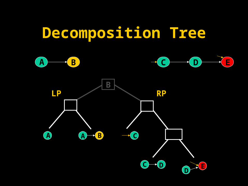
Decomposition Tree
A B C D E
A A B B C
C DD
BE
B

Decomposition Tree
A B C D E
A A B B C
C DD
BE
B

Decomposition Tree
A B C D E
A A B C
C DD
E
B

Decomposition Tree
A B C D E
A A B B C
C DD
BE
B

Decomposition Tree
A B C D E
A A B B C
C DD
BE
B
Decomposition Tree
A B C D E
A A B C
C DD
E
BLP RP

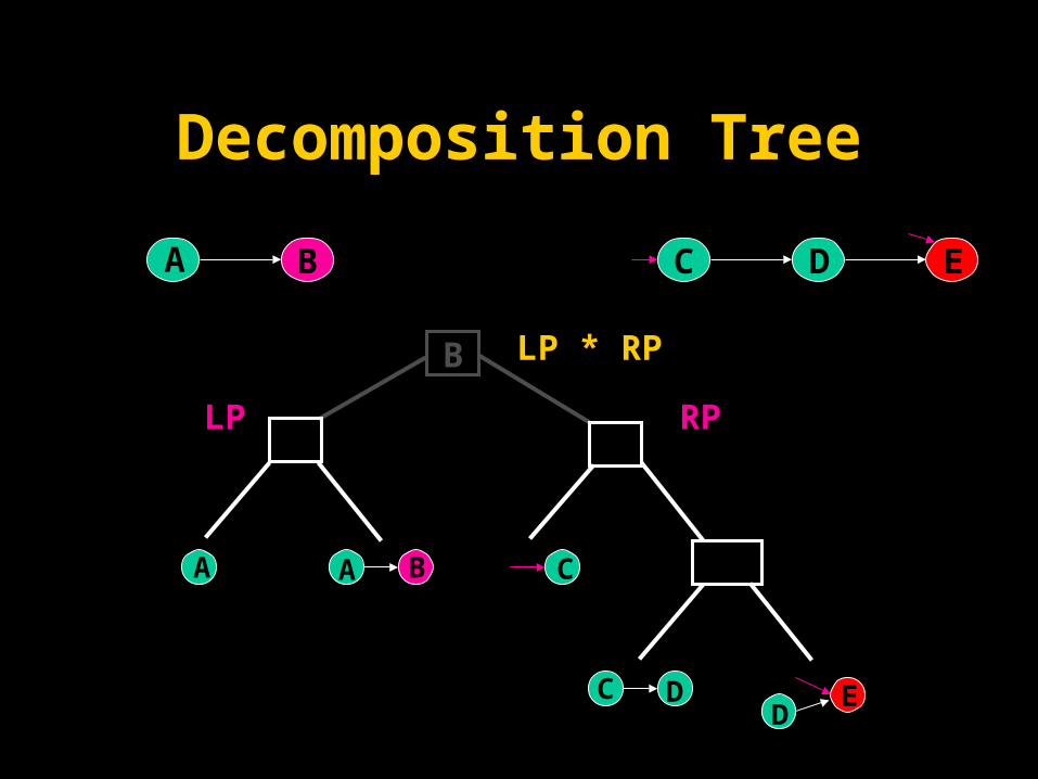
Decomposition Tree
A B C D E
A A B B C
C DD
BE
B LP * RP

Decomposition Tree
A B C D E
A A B B C
C DD
BE
B LP * RP
Decomposition Tree
A B C D E
A A B C
C DD
E
B LP * RP
LP RP

Decomposition Tree
A B C D E
A A B B C
C DD
BE
B LP * RP LP * RP

Decomposition Tree
A B C D E
A A B B C
C DD
BE
LP * RP + LP * RP

Dtrees
Generation from– Elimination orders– Jointree– hMeTiS hypergraph
partitioning program
a a’
.60 .40
b b’
a .90 .10
a’ .20 .80
d d’
c .50 .50
c’ .40 .60
e e’
bd .25 .75
bd’ .25 .75
b’d .90 .10
b’d’ .05 .95
c c’
b .70 .30
b’ .15 .85
A B C D
E
A C
B
D
• Cutset
B B
BC
• Context• Cluster
• Vars
A AB
AB BCDE
BC
CD BDE
BCDE

RC1
RC1(T,e)if T is a leaf node
return Lookup(T,e)
else p := 0
for each instantiation c of cutset(T)-E dop := p + RC1(Tl,ec) RC1(Tr,ec)
return p
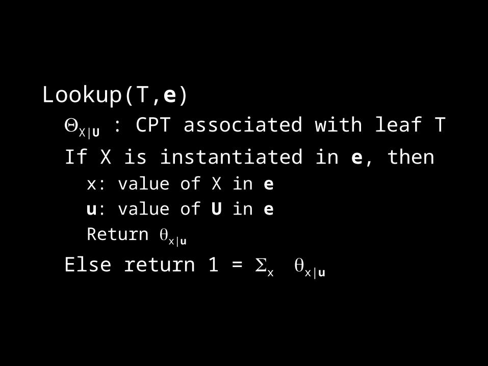
Lookup(T,e)X|U : CPT associated with leaf T
If X is instantiated in e, thenx: value of X in e
u: value of U in e
Return x|u
Else return 1 = xx|u
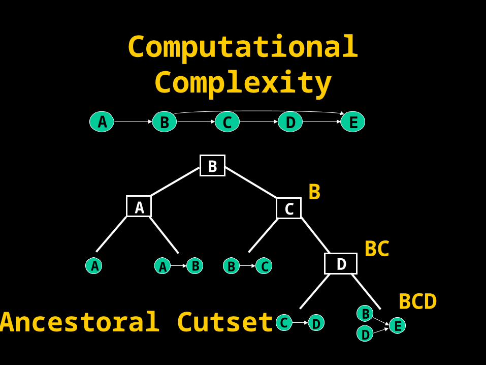
Computational Complexity
A B C D E
A A B B C
C DD
BE
A
B
C
D
B
BC
BCDAncestoral Cutset

Computational Complexity• Given
– DAG with n nodes– elimination order of width w
• Can construct a dtree in O(n log n) time:– Height O(log n)– cutset width <= w+1– a-cutset width O(w log n)
• Time complexity: O(n cw log n)
• Cutset Conditioning: O(n cs)

Network Effective Network
Size
Elimination-Order Width
Loop-Cutset Width
A-Cutset Width
1 Water 59.0 21.3 29.5 32.32 Midlew 108.4 19.7 39.3 45.93 Barley 138.0 21.8 57.3 51.14 Diabetes 1349.1 19.2 557.2 77.95 Link 922.7 28.0 347.0 70.76 Pigs 699.0 16.4 144.2 38.07 Munin1 410.3 26.4 122.6 51.78 Munin2 2202.7 20.0 495.9 54.69 Munin3 2293.4 16.3 454.2 51.1
10 Munin4 2313.4 19.7 521.5 51.9
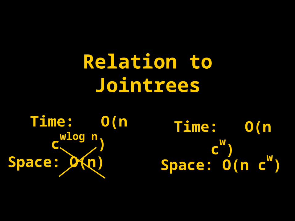
Relation to Jointrees
Time: O(n cw
)
Space: O(n)
Time: O(n cwlog n
)
Space: O(n cw
)

Decomposition Tree
A B C D E F
A
A B
B C
C D
D E E F
AB
CA B C

Decomposition Tree
A B C D E F
A
A B
B C
C D
D E E F
AB
C CC
.27
.39
ABCABCABCABC
ABC
ABCABC
ABC
A B C
Context(N)= A-Cutset(N)&Vars(N)

Decomposition Tree
A B C D E F
A
A B
B C
C D
D E E F
AB
C
D
E
A
B
C
D

RC2
RC2(T,e)if T is a leaf node, return Lookup(T,e)
y := instantiation of context(T)
If cacheT[y] <> nil, return cacheT[y]
p := 0
for each instantiation c of cutset(T)-E dop := p + RC2(Tl,ec) RC2(Tr,ec)
cacheT[y] := p
return p
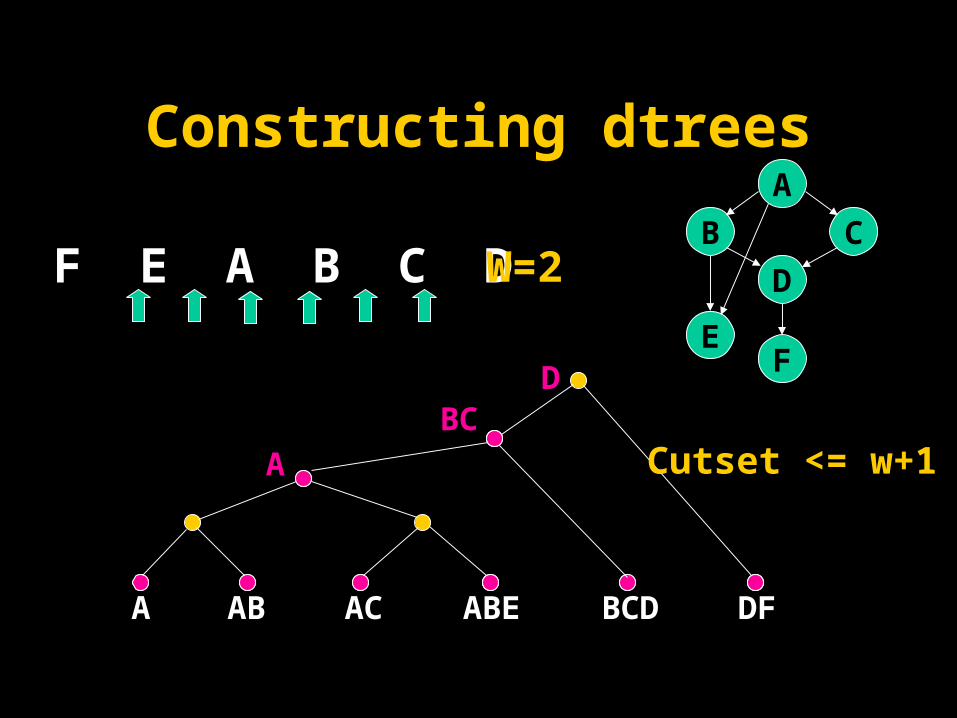
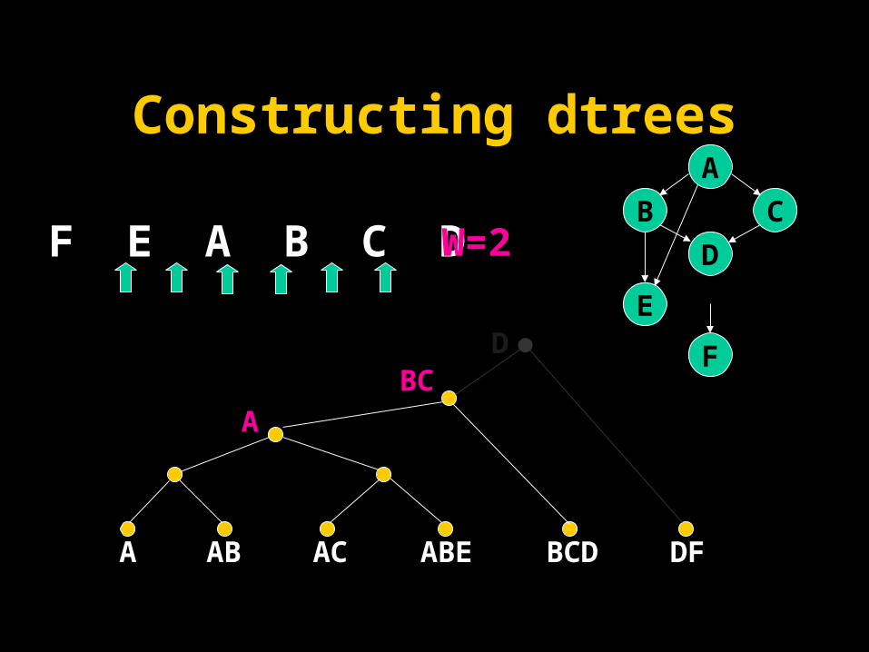
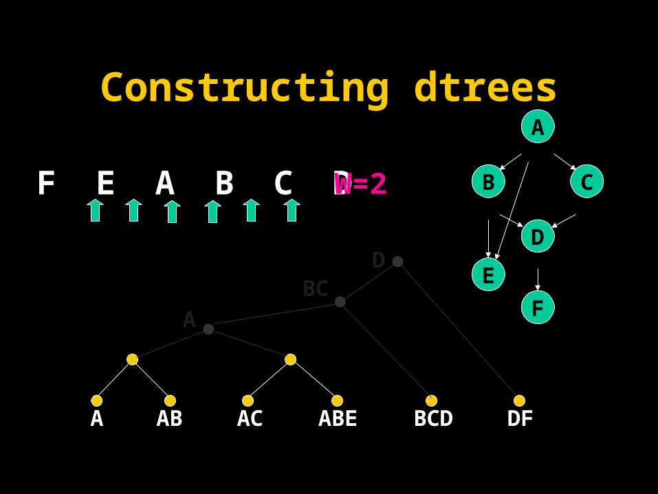
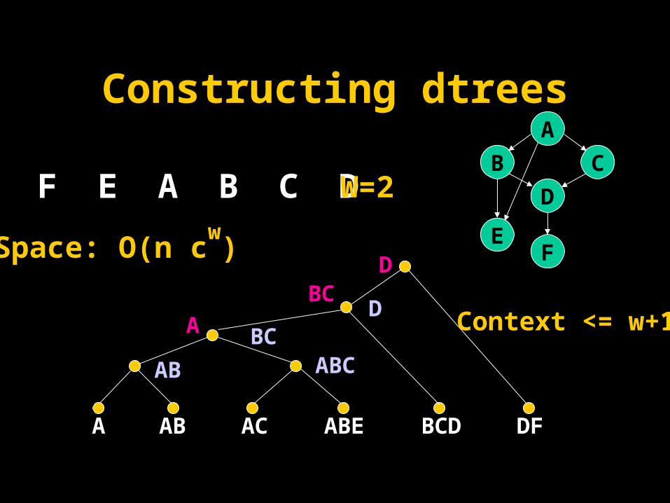
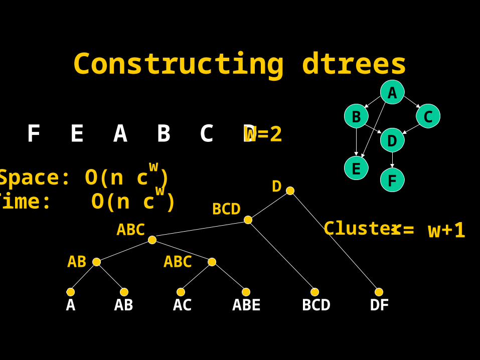
Constructing dtreesA
D
B
E
C
F
F E A B C D
A AB AC ABE BCD DF
DBC
A
W=2
Cutset <= w+1
Constructing dtreesA
D
B
E
C
F
F E A B C D
A AB AC ABE BCD DF
DBC
A
W=2

Constructing dtreesA
D
B
E
C
F
F E A B C D
A AB AC ABE BCD DF
DBC
A
W=2
Constructing dtreesA
D
B
E
C
F
F E A B C D
A AB AC ABE BCD DF
DBC
A
W=2
Constructing dtreesA
D
B
E
C
F
F E A B C D
A AB AC ABE BCD DF
DBC
A
W=2
DBC
AB ABC
Context <= w+1
Space: O(n cw
)
Constructing dtreesA
D
B
E
C
F
F E A B C D
A AB AC ABE BCD DF
D
BCDABC
W=2
AB ABC
Cluster<= w+1
Space: O(n cw
)Time: O(n c
w)

Constructing dtreesA
D
B
E
C
F
F E A B C D
ABE DF
BCDABC
W=2
Cluster<= w+1

Graphical Models
Elimination Order Jointree
Dtree

Hypergraph partitioningHypergraph partitioning
The problem of hypergraphpartitioning is well-studied
in VLSI design.….and is alive!
A hypergraph is a generalization of a graph, such that an edge is permitted to connect an arbitrary number of vertices, rather than exactly two.
The task of hypergraph partitioning is to find a way to split the vertices of a hypergraph into k approximately equal parts, such that the number of hyperedges connecting vertices in different parts is minimized.

An algorithm using hypergraph An algorithm using hypergraph partitioning to construct dtreespartitioning to construct dtrees
Given a DAG G, we first generate a hypergraph H that corresponds to G:
For each family F in G, we add a node NF to H. For each variable V in G, we add a hyperedge to H which connects all nodes NF such that V is a member of F.
Then we recursively invoke hypergraph partitioning to build a dtree:
The algorithm partitions the hypergraph into two sets of vertices, then recursively generates dtrees for each set, and finally combines the resulting dtrees into a new dtree (whose left child is the dtree for the first set, and whose right child is the dtree for the second set).
A AB
CDBC
A AB CDBC
A AB CDBC
For DAG:

A
CB
ED
F
HG
DFDF
AC ACE
EFH A AF
AB ABD
DFG
CC
EEHH
AAGG
BB
From dtrees to elimination ordersFrom dtrees to elimination orders

Any-Space Inference
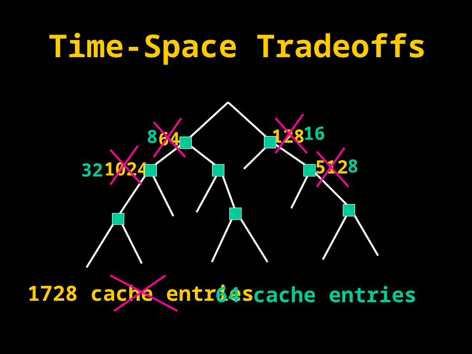
32
8 16
8
64 128
1024 512
1728 cache entries 64 cache entries
Time-Space TradeoffsTime-Space Tradeoffs
.8
0 1
.45
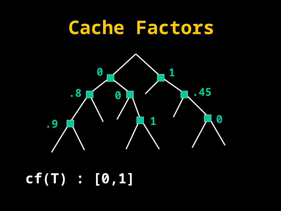
Cache FactorsCache Factors
.9 1 0
0
cf(T) : [0,1]

RC
RC(T,e)if T is a leaf node, return Lookup(T,e)
y := instantiation of context(T)
If cacheT[y] <> nil, return cacheT[y]
p := 0
for each instantiation c of cutset(T)-E dop := p + RC(Tl,ec) RC(Tr,ec)
If cacheT[y]? then cacheT[y] := p
return p

calls(T)=cutset#(Tp) [cf(Tp) context#(Tp) + (1-cf(Tp)) calls(Tp)]
When cf(T)=0 for every node T:
calls(T) = cutset#(Tp) calls(Tp)
When cf(T)=1 for every node T:
calls(T) = cutset#(Tp) context#(Tp) = cluster#(Tp)
exact count for discrete cache factors


Extension to Dgraphs
)(A )|( BD)|( BC)|( AB
Marginals
B

Dgraph
)(A )|( BD)|( BC)|( AB
AB
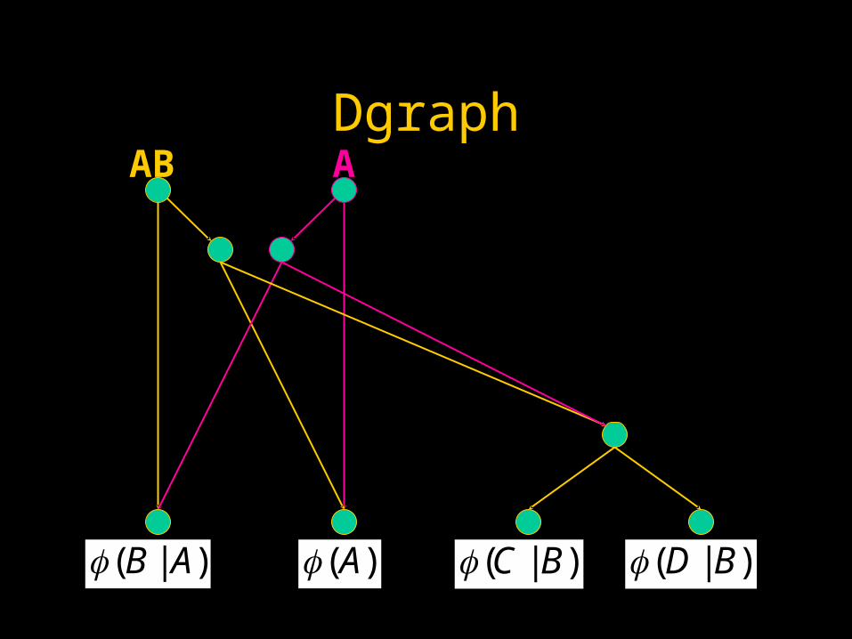
DgraphAB A
)(A )|( BD)|( BC)|( AB

Dgraph
)(A )|( BD)|( BC)|( AB
AB A BC

Dgraph
)(A )|( BD)|( BC)|( AB
AB A BC BD
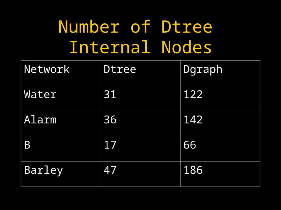
Number of Dtree Internal Nodes
Network Dtree Dgraph
Water 31 122
Alarm 36 142
B 17 66
Barley 47 186
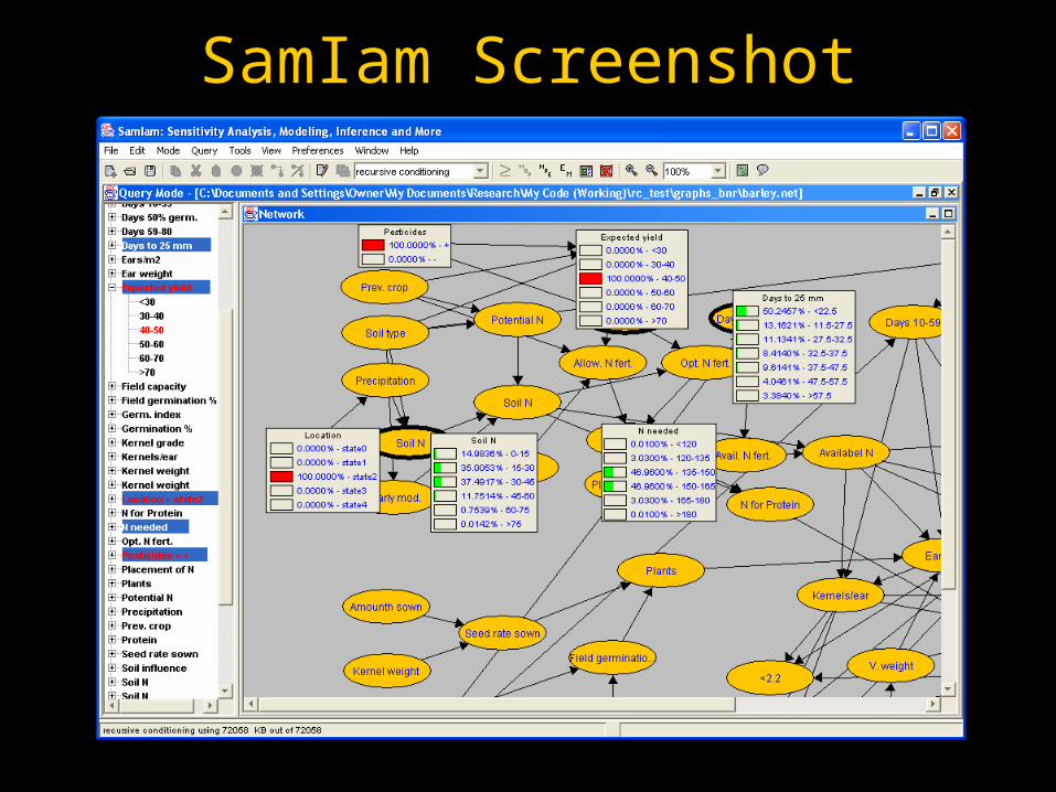
SamIam Screenshot

Discrete Cache Factor Search
• Problem– Given X MB of cache memory for RC– Find a discrete caching scheme which has a
minimal running time where the amount of memory used by all the dtree node caches is no larger than X

Number of RC Calls
• Can estimate running time of RC
• Function of: – dtree– cache factors
pt
ppppp tcallstcftcontexttcftcutsettcalls *1**)(##
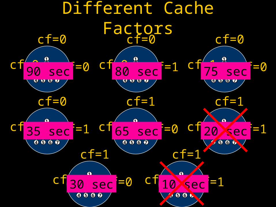
Different Cache Factors
1
2 3
4 5 6 7
cf=0
cf=1cf=01
2 3
4 5 6 7
cf=0
cf=0cf=0
1
2 3
4 5 6 7
cf=1
cf=0cf=01
2 3
4 5 6 7
cf=0
cf=1cf=1
1
2 3
4 5 6 7
cf=0
cf=0cf=1
1
2 3
4 5 6 7
cf=1
cf=1cf=0
1
2 3
4 5 6 7
cf=1
cf=0cf=11
2 3
4 5 6 7
cf=1
cf=1cf=1
20 sec65 sec35 sec
75 sec80 sec90 sec
30 sec 10 sec

Search Tree
1
2 3
4 5 6 7
cf=?
cf=?cf=?
1
2 3
4 5 6 7
cf=0
cf=?cf=?
No Caching
……
1
2 3
4 5 6 7
cf=1
cf=?cf=?
Full Caching
……
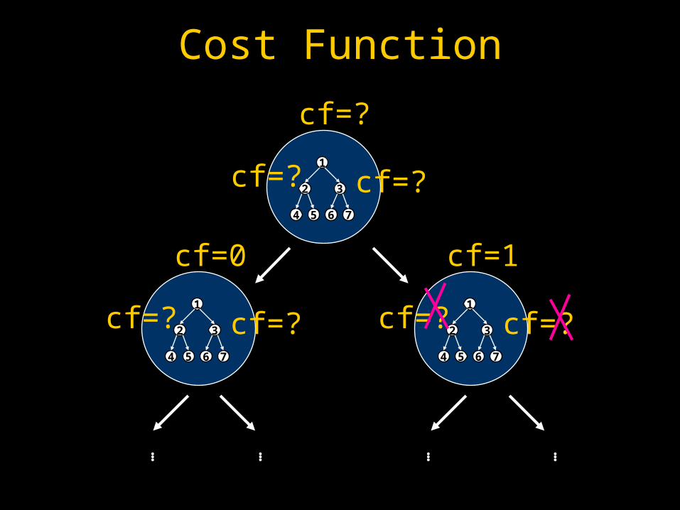
Cost Function
1
2 3
4 5 6 7
cf=?
cf=?cf=?
1
2 3
4 5 6 7
cf=0
cf=?cf=?1
2 3
4 5 6 7
cf=1
cf=?cf=?
… …… …

Cost Function
1
2 3
4 5 6 7
cf=?
cf=?cf=?
1
2 3
4 5 6 7
cf=0
cf=?cf=?1
2 3
4 5 6 7
cf=1
cf=1cf=1
… …… …
Admissible
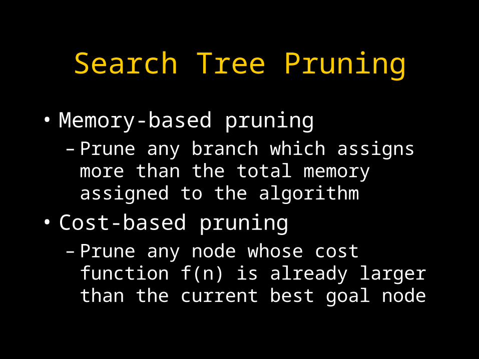
Search Tree Pruning
• Memory-based pruning– Prune any branch which assigns more than the
total memory assigned to the algorithm
• Cost-based pruning– Prune any node whose cost function f(n) is
already larger than the current best goal node

3.3 MB = 28 Sec7.6 MB = 12 Sec
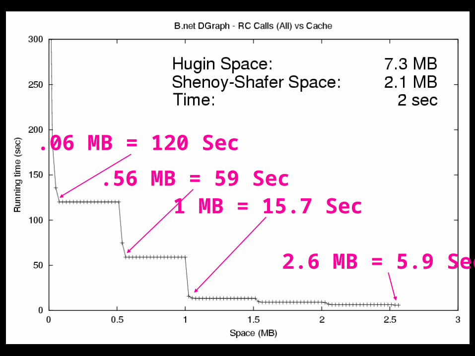
.56 MB = 59 Sec
2.6 MB = 5.9 Sec
1 MB = 15.7 Sec
.06 MB = 120 Sec

.19 KB = 2 Sec2.8 KB < .01 Sec.23 KB = .7 Sec

22 MB = 1 Min
6.5 MB = 4 Min

370 MB = 22 Min
150 MB = 5.8 Hours

400 MB = 18 Min
75 MB = 2 Hours
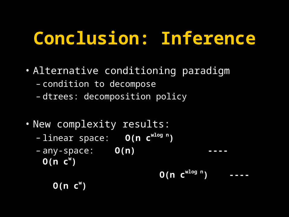
Conclusion: Inference
• Alternative conditioning paradigm– condition to decompose– dtrees: decomposition policy
• New complexity results:– linear space: O(n cwlog n)
– any-space: O(n) ---- O(n cw)
O(n cwlog n) ---- O(n cw)