recursion - stanford...

RecursionRecursion

Recursion Recursion Recursion

Recursion Recursion

CS209 Lecture-02: Spring 2009

Dr. Greg LavenderDepartment of Computer Sciences

Stanford [email protected]

Induction

Induction

Induction

InductionInduction

Induction

Induction

Types of Recursion

Recursive statements (also called self-referential)

Recursively (inductively) defined sets

Recursively defined functions and their algorithms

Recursively defined data structures and recursive algorithms defined on those data structures

Recursion vs Iteration

1

2Sunday, April 12, 2009

Recursive Statements

In order to understand recursion, one must first understand recursionThis sentence contains thirty-eight lettersGNU = GNU’s Not Unix!

The Ouroboros is an ancient symbol implying self-reference

or a “vicious circle”

Paradoxical Statements

This is not a pipe

The Barber Paradox

A barber shaves all and only those men who do not shave themselves

if the barber does not shave himself, he must shave himself

if the barber does shave himself, he cannot shave himself

The Treachery of Images (1928-29),by René Magritte

3


The “Quine” ProblemJust as there are self-referential statements in English, you can write a self-reproducing program in a programming language, which is called a “quine” after the Harvard logician W. V. O. Quine.

A quine is a program that accepts no input and outputs an exact syntactic replica of itself

As a corollary to a famous theorem called Kleene’s (second) Recursion Theorem, or the “Fixed Point” Theorem, there exist many such programs. Try writing one in your favorite language. Here’s the start of one in C:

int main() { printf(“int main() { printf( ...

Recursion is Definitely Odd!

Or is it Even?!

odd n = if (n == 0) then False else even (n-1)

even n = if (n == 0) then True else odd (n-1)

© M. C. Escher

5


Induction vs Recursion

For beginners, induction is intuitive, but recursion is often counter-intuitive

Induction is like “ascending”

e.g., counting up: 1,2,3,...

Recursion is like “descending”

e.g., counting down: n,n-1,n-2,...

But they often go hand-in-hand to solve a problem

Lost in Recursion LandBeginners often fail to appreciate that a recursion must have a conditional statement or conditional expression that checks for the “bottom-out” condition of the recursion and terminates the recursive descent

We call the bottom-out condition the “base case” of the recursion

If you fail to do this properly, you end up lost in Recursion Land and you never return!

7


A Simple Algebraic Proof

Due to Carl Friedrich Gauss (1777-1855)

he was told to sum the first 100 positive integers at a young age while in a class on arithmetic

Gauss combined counting up with counting down

(1 + 2 + 3 + ... + n) + (n + n-1 + n-2 + ... + 1) = (1+n) + (2+n-1) + (3+n-2)... + (n+1) = n+1 + n+1 + n+1 + ... + n+1 = n * (n+1) = 2 * sum(n)

Therefore, sum(n) = n*(n+1)/2 for all n >= 1

Ex: sum(100) = (100 * 101)/2 = 50*101 = 5050

Summing Up vs Summing Down

a well-ordered ascending sequence

isum(n) = 1 + 2 + 3 + ... + n

a well-ordered descending sequence

rsum(n) = n + n-1 + n-2 + ... + 1

Both isum and rsum compute the same value for a given n, but isum does so in O(1) stack space while rsum requires O(n) stack space

// inductive sum (count up)int isum(int n) { int sum = 0;

for (int i=1; i<=n; ++i) sum += i; return sum;

}

// recursive sum (count down)int rsum(int n) { assert(n > 0); if (n == 1)

return 1; else

return n + rsum(n-1);}

9


Inductive SetsThe set of Sponges is the smallest set satisfying the following rules, known as the Sponge Bob Axioms:

Bob is a Sponge

If s is a Sponge, then the successor of s is a Sponge.

Bob is not the successor of any Sponge

Induction Axiom: For all sets S, if Bob is in S and for every Sponge s in S, the successor of s is in S, then every Sponge is in S

A recursively defined abstract data type that captures this inductive set:

data Sponge = Bob | Succ Sponge

Peano ArithmeticUsing the Sponge Bob Axioms, we can define arithmetic on the Natural Numbers, but let’s equate the data type Sponge to ‘Nat’ and Bob to ‘Zero’. We then define Peano Arithmetic, named after Guiseppe Peano (1858-1932), who defined the set Nat inductively using such axioms (called Peano’s Axioms of course)

-- inductive “Nat” data type-- Ex: Zero, Succ(Zero), Succ(Succ(Zero)) ...-- i.e., counting up: 0,1,2,...

data Nat = Zero | Succ Nat derivin (Ord, Show) -- boolean function to test for the base caseiszero :: Nat -> Booliszero Zero = Trueiszero (Succ n) = False

11


Basic Arithmetic FunctionsArithmetic can then be defined recursively in terms of counting up (successor) and counting down (predecessor)succ, pred :: Nat -> Nat -- unary functions

succ n = Succ n -- count up by prepending Succ to npred (Succ n) = n -- count down by removing a Succ from npred Zero = error “no predecessor of Zero”

add, mult :: (Nat, Nat) -> Nat -- binary functions

add (n, Zero) = nadd (Zero, m) = madd (n, m) = succ(add(n, pred m)) -- succ of n, m times

mult (n, Zero) = Zeromult (Zero, m) = Zeromult (n, m) = add(n, mult(n, pred m)) -- succ of n, n+m times

ExampleA calculator using Peano Arithmetic:

PA> pred Zero*** Exception: no predecessor of Zero

PA> succ ZeroSucc (Zero)

PA> pred (Succ Zero) Zero

PA> add(Succ Zero, Succ (Succ Zero))Succ (Succ (Succ (Zero)))

PA> add(Succ Zero, Succ (Succ (Succ (Succ Zero))))Succ (Succ (Succ (Succ (Succ (Zero)))))

PA> mult(Succ (Succ Zero), Succ (Succ (Succ (Succ Zero))))Succ (Succ (Succ (Succ (Succ (Succ (Succ (Succ(Zero))))))))

13


Classic Recursive Functions

Euclid’s Greatest Common Divisor (GCD) function

Factorial function

Fibonacci function

Euclid’s GCD Function

The Greatest Common Divisor (GCD) of a pair of integers (x, y) is defined by taking the remainder r of (abs x) divided by (abs y). If r is 0, return x. Otherwise compute GCD of y and r.

gcd :: (Int, Int) -> Intgcd (x, y) = gcd’ (abs x) (abs y) where gcd’ x 0 = x gcd’ x y = gcd’ y (x mod y)

gcd (-98, 16) = gcd’ 16 (98 mod 16) = gcd’ 16 2 = gcd’ 2 (16 mod 2) = gcd’ 2 0 = 2

15


Factorial FunctionA recursive factorial algorithm implementing the function n! first counts down from n to 0 by recursively descending to the bottom-out condition, then performs n multiplications as the recursion ascends back up.

0! = 1 n! = n * (n-1)! for all n > 0

fact :: Integer -> Integerfact n | n == 0 = 1 -- base case terminates recursion | n > 0 = n * fact (n-1) | otherwise = error “fact: negative value for n”

fact 3 => 3 * fact(2) => 3 * (2 * fact(1)) => 3 * (2 * (1 * fact(0))) => 3 * (2 * (1 * 1)) =>3 * (2 * 1) => 3 * 2 => 6

Fibonacci FunctionThe Fibonacci numbers are an infinite sequence of numbers 0,1,1,2,3,5,8,13,21,... named after Leonardo of Pisa, aka Leonardo Fibonacci (1170-1250), in which each item is formed by adding the previous two, starting with 0 and 1, i.e., 0+1->1, 1+1->2, 1+2->3, 2+3->5

The Fibonacci function can be defined recursively as: fib :: Integer -> Integer fib 0 = 0 fib 1 = 1 fib n = fib(n-2) + fib(n-1)

Notice that in computing fib n, there are two recursive calls that are duplicative in the sense that computing fib(n-1) necessarily computes fib(n-2) all over again. This kind of “double” recursion is terribly inefficient.

17


Lists are Recursive StructuresA list is a recursively defined data type with elements of some type ‘a’, e.g., [1,2,3] is a list of type ‘int’

[] constructs the empty list; ‘:’ is an infix right associative list constructor operator (cons), that constructs a new list from an element of type ‘a’ on the left and a list [a] on the right

data [a] = [] | a : [a]

3:[] = [3]; 2:[3] = [2,3]; 1:[2,3] = [1,2,3] = 1:2:3:[]

let head [a1,a2,...,an] = a1; tail [a1,a2,...,an] = [a2,...,an]head [] = error; tail [] = error

let (h:t) pattern match [a1,a2,...,an] such that h = a1, t = [a2,..,an]

let ‘++’ be list concatenation: [1,2] ++ [3,4] = [1,2,3,4]

List Comprehensions

Another way to construct a list is using a list comprehension, similar to a set comprehension in Set Theory

Set Theory: { f(x) | x in S}, {x | p(x), x in S }

Haskell: [f x | x <- xs], [ x | x <- xs, p(x) ]

Example: map :: (a -> b) -> [a] -> [b] map f xs = [ f x | x <- xs ] map square [1,2,3] => [1,4,9]

filter :: (a -> bool) -> [a] -> [b] filter p xs = [ x | x <- xs, p x] cprod :: [a] -> [b] -> [(a,b)] cprod xs ys = [(x,y) | x <- xs, y <- ys]

19


Recursive List Functionslength :: [a] -> Int -- [a] means a list of any type ‘a’length [] = 0 -- empty list is the base caselength (h:t) = 1 + length t

sum :: (Num a) => [a] -> Int -- type of a must be subtype of Numsum [] = 0 -- empty list is the base casesum (h:t) = h + sum t

mean :: (Num a) => [a] -> Floatmean lst = sum lst / length lst

-- Note: mean above requires 2 traversals of the list!-- Can we compute the mean using just one traversal? -- let (x,y) be an ordered pair and fst (x,y) = x, snd (x,y) = y

sumlen :: (Num a) => [a] -> (Int,Int) -> (Int,Int)sumlen [] = psumlen (h:t) p = sumlen t (h + fst(p), 1 + snd(p))

mean lst = fst(p) / snd(p) where p = sumlen lst (0,0)

Recursive List Functions-- list concatenation infix operator(++) :: [a] -> [a] -> [a] [] ++ ys = ys(x:xs) ++ ys = x : (xs ++ ys)

Ex: [1,2,3] ++ [4,5,6] => [1,2,3,4,5,6]

-- index infix operator, starting at index 0(!!) :: [a] -> Int -> axs !! n | n<0 = error "Prelude.!!: negative index"[] !! _ = error "Prelude.!!: index too large"(x:_) !! 0 = x(_:xs) !! n = xs !! (n-1

Ex: [1,2,3,4,5] !! 4 => 5

take :: Int -> [a] -> [a]take n _ | n <= 0 = []take _ [] = []take n (x:xs) = x : take (n-1) xs

Ex: take 5 [1..] => [1,2,3,4,5]

21


Recursive List Functionsiterate :: (a -> a) -> a -> [a]iterate f x = x : iterate f (f x)

Ex: iterate (+1) 1 => [1,2,3,4,5,6,7,8,9,10,...]

repeat :: a -> [a]repeat x = xs where xs = x:xs

Ex: repeat “ATCG” => [“ATCG”, “ATCG”, “ATCG”, ...]

replicate :: Int -> a -> [a]replicate n x = take n (repeat x)

Ex: replicate 5 "ATCG" => ["ATCG","ATCG","ATCG","ATCG","ATCG"]

cycle :: [a] -> [a]cycle [] = error "Prelude.cycle: empty list"cycle xs = xs' where xs' = xs ++ xs'

Ex: cycle ['A','T','C','G'] => "ATCGATCGATCGATCGATCGATCGATCG...

Folding over a ListGiven the recursive structure of a list based on the cons operator “:” we can iterate over a list and substitute another operator between the elements and “collapse” the list to a value (which may be another list)

foldl :: (a -> b -> a) -> a -> [b] -> afoldl f z [] = zfoldl f z (x:xs) = foldl f (f z x) xs

foldl (+) 0 [1,2,3,4,5] => 0+1+2+3+4+5 => 15foldl (*) 1 [1,2,3,4,5] => 1*1*2*3*4*5 => 120sum,prod :: [Int] -> Intsum xs = foldl (+) 0 xsprod xs = foldl (*) 1 xs

foldl1 :: (a -> a -> a) -> [a] -> afoldl1 f (x:xs) = foldl f x xs

foldl1 (*) [1,2,3,4,5] => 120

23


Mapping over a ListMap applies a function to each element of type ‘a’ of a list, producing a list of type ‘b’ values. Type ‘a’ may equal ‘b’

map :: (a -> b) -> [a] -> [b]map f (x:xs) = f x : map f xs-- or with a list comprehension: [f x | x <- xs]

-- map any function of type (a->b) across a listmap length [[],[1,2,3],[‘A’,‘C’,‘T’,’G’] => [0,3,4]map even [1,2,3,4,5] => [False,True,False,True,False]map Char.ord [‘A’,’T’,’C’,’G’] => [65,67,84,71]

-- (+5) is called a “section” -- (+) :: a->a->a but (+5),(5+) :: a->amap (+5) [1,2,3,4,5] => [6,7,8,9,10]map (5+) [1,2,3,4,5] => [6,7,8,9,10]

-- (\x -> x * x) is an anonymous “lambda” functionmap (\x -> x * x) [1,2,3,4,5] => [1,4,9,16,25]

A Recursive List Fibonacci

With “lazy lists” we can take a different approach

fibs :: [Integer]fibs = 0 : 1 : zipWith (+) fibs (tail fibs)

fiblist :: Int -> [Integer]fiblist n = take n fibs

fib :: Int -> Integer fib n = fibs !! (n-1)

This is a recursive mind-twister! What is going on?

zipWith :: (a->b->c) -> [a] -> [b] -> [c]zipWith z (a:as) (b:bs) = z a b : zipWith z as bszipWith _ _ _ = []

25


Polynomial Evaluation

Given a n-degree polynomial P of the form:

Pn(x) = anxn + an-1xn-1 + ... a1x + a0

A naive evaluation requires at most n additionsBUT, n+1 + n + n-1 + ... + 1 = (n2+n)/2 multiplications

Can we do better? Yes, factor out the duplicate multiplications required for each xi

Pn(x) = (((...(an x + an-1) ... )x + a2)x + a1)x + a0

Requires n additions, but only n multiplications!

Horner’s MethodDescribed by the Englishman George Horner in 1819, but known to Isaac Newton as early as 1669.

Pn(x) = (((...(an x + an-1) ... )x + a2)x + a1)x + a0

Leads to a natural recursive definition:let Pn(x) = Hn(x) where H0(x) = a0

Hi(x) = Hi-1(x) * x + ai, for i = 1,2,...,n

p :: (Num a) => a -> [a] -> ap x coeffs = h x (reverse coeffs) where h x (a:[]) = a h x (a:as) = (h x as) * x + a

27


Branching Recursion

“Divide & Conquer” strategy

split a problem into two or more sub-problems; solve each sub-problem recursively; then combine the sub-results to obtain the final answer

Classic examples

binary tree traversal

sorting a list of numbers © M. C. Escher

Branching Recursion

1

2

3 4 6 7

5

Binary Tree

Root

RightSubtree

LeftSubtree

Leaf Leaf

Root

Root

Leaf Leaf

Preorder Traversal: [1, 2, 3, 4, 5, 6, 7] Inorder Traversal: [3, 2, 4, 1, 6, 5, 7]Postorder Traversal: [3, 4, 2, 6, 7, 5, 1]

29


Recursive Binary Tree Traversal Algorithms

data BinTree a = Leaf a | Root a (BinTree a) (BinTree a)

preorder :: BinTree a -> [a]preorder (Leaf v) = [v]preorder (Root v l r) = [v] ++ preorder l ++ preorder r

inorder :: BinTree a -> [a]inorder (Leaf v) = [v]inorder (Root v l r) = inorder l ++ [v] ++ inorder r

postorder :: BinTree a -> [a]postorder (Leaf v) = [v]postorder (Root v l r) = postorder l ++ postorder r ++ [v]

Simple Recursive SortingGiven a list of values of type ‘a’ on which there is an ordering relation defined, permute the elements of the list so that they are ordered in either ascending or descending order

Example: Given the input list [16, -99, 25, 71, 9, 3, 28], sort it into ascending order

Step 1: select the first element of the list as a “pivot”

Step 2: partition the list into two sublists “left” and “right” where left = [ x | x <= pivot] and right = [ y | y > pivot]

Step 3: Recursively sort the left sublist and prepend that result to the singleton list [pivot], and recursively sort the right sublist and append the result to the left++pivot list

31


Recursive Sorting Examplesort [16, -99, 25, 71, 9, 3, 28]

sort [-99,9,3] ++ [16] ++ sort [25,71,28]

(sort [] ++ [-99] ++ [9,3]) ++ [16] ++ sort [25,71,28]

(sort [] ++ [-99] ++ sort [9,3]) ++ [16] ++ sort [25,71,28]

(sort [] ++ [-99] ++ (sort [3] ++ [9] ++ sort []) ++ [16] ++ sort [25,71,28]

[-99, 3, 9] ++ [16] ++ sort [25,71,28]

[-99, 3, 9] ++ [16] ++ (sort [] ++ [25] ++ sort [28, 71]) [-99, 3, 9] ++ [16] ++ (sort [] ++ [25] ++ (sort [] ++ [28] ++ sort [71])

[-99, 3, 9, 16, 25, 28, 71]

[-99, 3, 9] ++ [16] ++ [25, 28, 71]

Recursive Sort Algorithm

Polymorphic recursive sorting function that sorts a list of elements of type ‘a’, where ‘a’ is required to be ordered (i.e., has the relational operators ==, <, >, <= and >= defined)

sort :: (Ord a) => [a] -> [a]

sort [] = [] -- base casesort (x:[]) = [x] -- singleton listsort (pivot:rest) = sort left ++ [pivot] ++ sort right where left = [x | x <- rest, x <= pivot] right = [y | y <- rest, y > pivot]

33


Recursion vs IterationIterative factorial requires O(1) stack space

update n and m in place within one stack activation frame each time through the loop

int ifact (int n) { int m = 1; while (n > 1) { m = m * n; n = n-1; } return m;}

n=3m=1

n=3-1m=1*3

Frame #1 Frame #1 Frame #1n=2-1m=3*2

Recursion vs IterationRecursive factorial requires O(n) stack space

“Count down” from n and delay doing any multiplications until the recursion bottoms out, then do the multiplications on the way “back up”

int rfact (int n){ return (n == 0 || n == 1) ? 1 : n * fact(n-1);}

n = 3

n = 2

n = 1

delay 3 * fact(2)

delay 2 * fact(1)

recursion bottoms out at 1

Frame #1

Frame #2

Frame #3

35


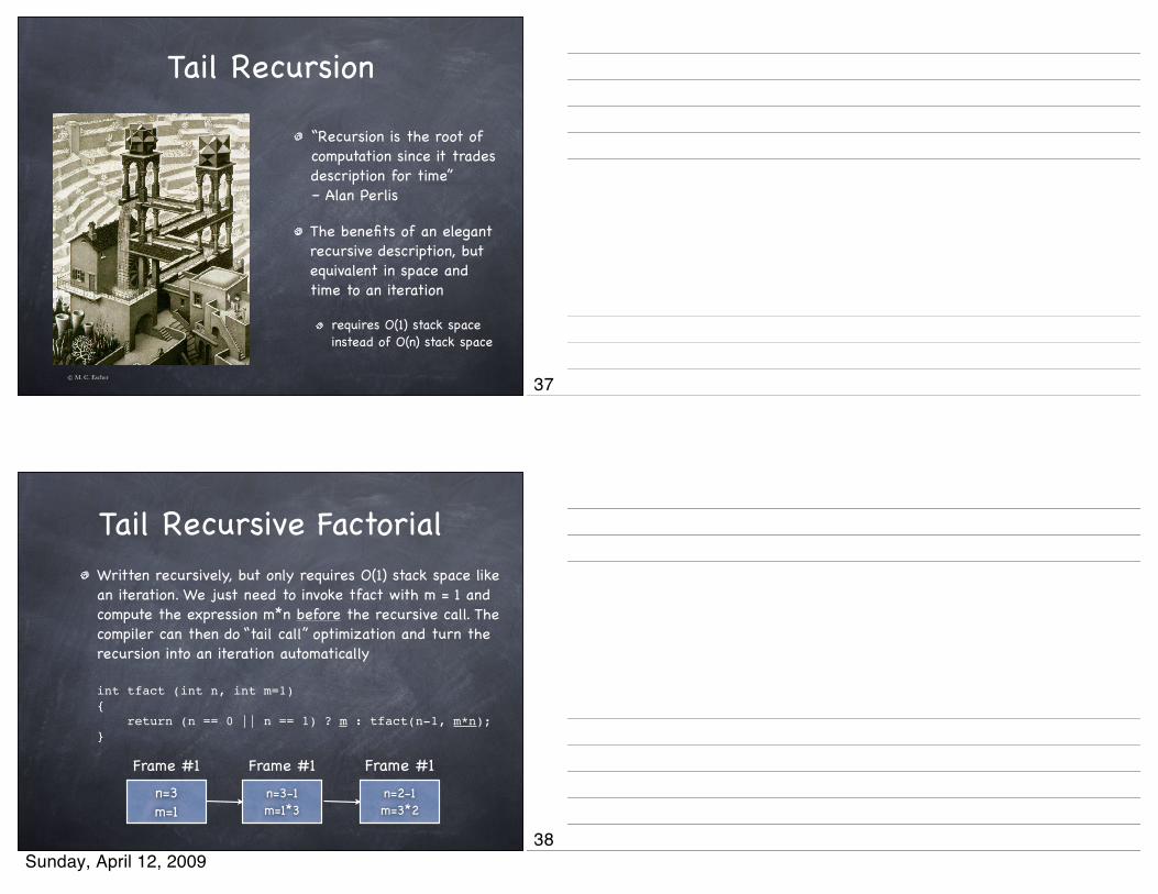
Tail Recursion

“Recursion is the root of computation since it trades description for time” – Alan Perlis

The benefits of an elegant recursive description, but equivalent in space and time to an iteration

requires O(1) stack space instead of O(n) stack space

© M. C. Escher

Tail Recursive FactorialWritten recursively, but only requires O(1) stack space like an iteration. We just need to invoke tfact with m = 1 and compute the expression m*n before the recursive call. The compiler can then do “tail call” optimization and turn the recursion into an iteration automatically

int tfact (int n, int m=1){ return (n == 0 || n == 1) ? m : tfact(n-1, m*n);}

n=3m=1

n=3-1m=1*3

Frame #1 Frame #1 Frame #1n=2-1m=3*2

37


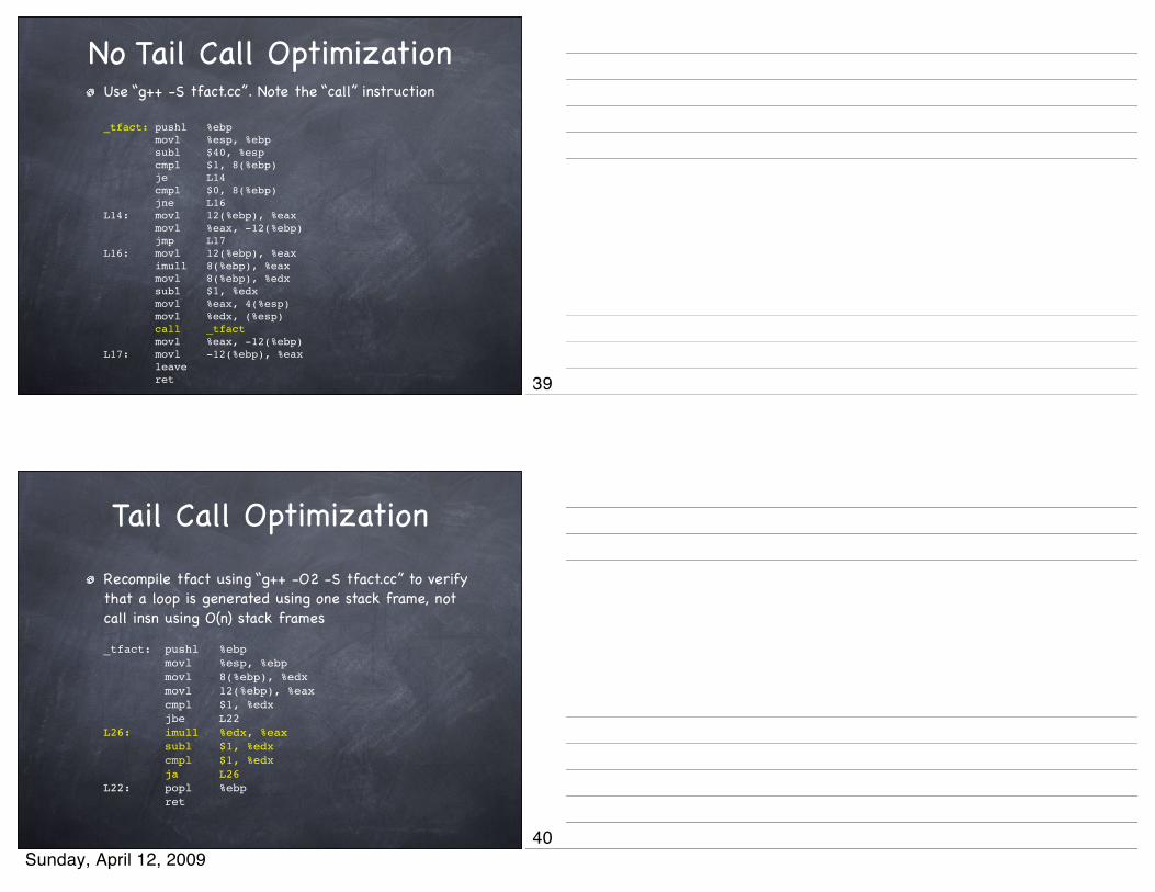
No Tail Call OptimizationUse “g++ -S tfact.cc”. Note the “call” instruction

_tfact: pushl %ebp movl %esp, %ebp subl $40, %esp cmpl $1, 8(%ebp) je L14 cmpl $0, 8(%ebp) jne L16L14: movl 12(%ebp), %eax movl %eax, -12(%ebp) jmp L17 L16: movl 12(%ebp), %eax imull 8(%ebp), %eax movl 8(%ebp), %edx subl $1, %edx movl %eax, 4(%esp) movl %edx, (%esp) call _tfact movl %eax, -12(%ebp)L17: movl -12(%ebp), %eax leave ret

Tail Call Optimization

Recompile tfact using “g++ -O2 -S tfact.cc” to verify that a loop is generated using one stack frame, not call insn using O(n) stack frames _tfact: pushl %ebp movl %esp, %ebp movl 8(%ebp), %edx movl 12(%ebp), %eax cmpl $1, %edx jbe L22L26: imull %edx, %eax subl $1, %edx cmpl $1, %edx ja L26L22: popl %ebp ret

39


Tail Recursion in Haskell

Factorialfact n = tfact n 1 where tfact 0 m = 1 tfact n m = tfact (n-1) (m*n)

Reverse a listreverse [] = []reverse xs = rev xs [] where rev [] ys = ys rev (x:xs) ys = rev xs x:ys

Is foldl tail recursive?reverse xs = foldl (flip (:)) [] xs where flip f x y = f y x

Recommended ReadingRecursion Theory and Logic:

Computability and Logic, 4th Ed., by George Boolos, et al.

Topical articles at http://plato.stanford.edu and Wikipedia

Recursive Programming:

“Recursive Functions of Symbolic Expressions and their Computation by Machine (Part I),” by John McCarthy (see his website)

Thinking Recursively, 2nd Ed., by Eric Roberts

Recursive Programming Techniques, by W. H. Burge

Programming in Haskell, by Graham Hutton

41


Other Fun Reading

Godel, Escher, Bach, by Douglas Hofstadter

Books by Raymond Smullyan

What is the Name of this Book?

To Mock a Mockingbird

Forever Undecided

Recursion Theory for Metamathematics (advanced)

Life Itself is Recursive, So Self-Reflect On It!

© M. C. Escher

43


recursion - stanford...

Documents