Rectification of Circles, Spheres, and Classical Geomet ries

Farz-Ali Izadi

A thesis submitted in conformity with the requirements

for the degree of Doctor of PhiIosophy

Graduate Depart ment of hjIathemat ics

University of Toronto

@ Copyright by Fan-Ali Izadi (2001)

National Library Ifl ofCanada Bibliothèque nationale du Canada

Acquisitions and Acquisitions et Bibliographie Services services bibliographiques 395 WeUington Street 395. nie Wellington Ottawa ON Kt A ON4 Ottaw ON K I A ON4 canada Canada

The author has granted a non- exclusive licence allorving the National Library of Canada to reproduce, losn, distri'bute or seil copies of this thesis in microfixm, paper or electronic formats.

The author retains ownership of the copyright in this thesis. Neither the thesis nor substantial extracts f?om it may be printed or othemise reproduced without the author's permission.

L'auteur a accordé me licence non exclusive pennettant à la Bibliothèque nationale du Canada de reproduire, prêter, distribuer ou vendre des copies de cette thèse sous la fome de microfiche/fïlm, de reproduction sur papier ou sur format électronique.

L'auteur conserve la propriété du droit d'auteur qui protège cette thèse. Ni la thése ni des extraits substantiels de celle-ci ne doivent être imprimés ou autrement reproduits sans son autorisation.

Abst ract Rectification of Circles, Spheres, and Classical

Geomet ries Ph.D. 2001

Farz- Ali Izàdi

Depart nient of Mat heniat ics

University of Toronto

The goal of this thesis is to describe al1 local diffeomorphisms niapping a collec-

t ion of circles (res. spheres) in a neighborhood into straight lines (res. hyperspaces).

This description contains two main results. The first is a complete description of

the generat rectifiaùle collection of circles in R y o r sphereS of codimension 1 or 2 in

Rn) passing through one point. Ir turns out t hat to be rectifiable al1 circles (or al1

spheres) need to pass through sorne other cornmon point. The second main result

is a complete description of geornetries in which al1 the geodesics are circles. This

is a consequence of an extension of the Beltrami theorem by replacing straight lines

wit h circles.

Acknowledgement s

1 would like to thank my supenisor. Prof. Askold G. K h o v s k i i . for his guidance

in this work. It bas been pieasure working Mth him. Askold's patience. kindness.

arid ericouriigenierit are wctrully appreciated.

1 am also grateful to my cornmittee niembers Prof. K. Moore (Physics). Prof.

T. Blooru, Prof. 1. Graham. Prof. E. Sleinrenken. and especiall>* Prof. R. Sharpe

and Prof. A. Gabrielov (Purdue University) for Iiaving read iny thesis and for ~hei r

valuable suggestions for improving the presentation of the t hesis.

Sly thanks go to nly good friends K. Kaveli and V. Tirnorin for niany discussions.

shnring ideas and reading of the first draft of the thesis.

1 gratefully acknowledged the scholarship froni the Iranian llinistry of Science

and technology. and also the Slathematics Department of the University of Toronto

durinp my graduate study.

Many thanks go to the staff of the Department for their assistance. and especially

to Ida Bulat. the Graduate Secretary of the Department. for al1 her kindly help

during my study here.

Above d l . 1 would like to offer my thanks to God. for His faithfulness and

goodness t o me. Without Him. This work could not have been completed.

Contents

1 Summary of Results 3

. . . . . . . . . . . . . . . . . 1.1 Application in Riemannian Geometry. 3

. . . . . . . . . . . . . . . . 1.2 Rectification and Riemannian Geometry 5

. . . . . . . . . . . . . . . . . . . . . . . . . . . . . . . . 1.3 Main results 5

. . . . . . . . . . . . . . . . . . . . . . 1.4 Rich Families of Circles in R3 9

2 Fundamental Theorems 11

. . . . . . . . . . . . . . . . 2.1 Rectification of a Bundle of Circles in R3 11

. . . . . . . . . . . . . . . 2.2 Rectification of a Biindle of Spheres in Rn 19

3 Classification Theorems 27

. . . . . . . . . . . . . . . . . . . . . . 3.1 Rich Families of Circles in R3 25

4 Applications in Riemannian Geometry 35

. . . . . . . . . . . . . . . . . . . . . . . . . . 4.1 Riemannian Geometry 36

. . . . . . . . . . . . . . . . 4.2 Rectification and Riemannian Geornetry 39

A Preliminary Concepts 41

. . . . . . . . . . . . . . . . . . . . . . . . A . 1 Finite Difference Calculus 41

. . . . . . . . . . . . . . . . . . . . . . . . . . . A 2 Projective Geometry 43

. . . . . . . . . . . . . . . . . . . . . . . . A.3 Some Xecessary Theorems 47

PREFACE

By a rectification of a faniily of circles (res. spheres). we simply mean a local diffeo-

morphism mapping it into straight lines (res. hyperspaces). Our goal is to describe

such diffeoniorphisms ivhenever t hey exist . This descript ion cont aiiis two main re-

sults. The first is a complete description of general (and big enough) rectifiable

collections of circles in R3 (or spheres of codimension 1 or 2 in Rn) passing tlirough

one point. It turns out that to be rectifiable al1 circles (or al1 spheres) need to pass

through some other common point. The second result is a coniplete description

of geometries in which al1 the geodesics are circles. These are classical geonietries

(hyperbolic. Euclidean. and Ellipt ic).

The problem that author solved has its origin in .Vornography ': how to reduce

a nomogram of aligned points to a circulw nomogram?[l! In more niathematical

terms: what are local diffeomorphisms that send germs of lines to gernis of circles?

This question was initially posed For Zdimensional nomograms (by G.S. Khownskii)

and solved by A.G. Kho~ansMi in that case. ûur resuk teads to a soiution of the

corresponding Sdimensional Xomography. On the ot her hand. it is a continuation

of the Mobius' classical works that describe all transformations taking Lines to lines

and circles to circles. This work is also related to Beltrami's investigations. By

Beltrami's classical theorem al1 the geometries whose geodesics are straight tines

have constant curvature. We proved that al1 geometries in R3 whose geodesics are

'A discipline tvhich has discovered by a. French Civil Engineer. Docagne (1880) and it turns out

to have practical applications in many branches of science and technology [8.9]

circles niust also have constant curvature (in P this is wrong). We gave also a

complete description of al1 such metrics.

This dissertation consists of 4 Chapters and an Appendk. Chapter 1 is a brief

discussion of the niain results and some related remarks. In Chapter 2. we first

give die precise defiriitious of rectificatiuri for Lu th cullectioii uf circlea arid splieres

passing throiigh one point and then we prove their fundamental theorems. These

give us the first main result.

Chapter 3 is devoted to the classification t heorems for t lie rich families ' of circles

i.e. the families of circles tha t look like the farnilies of geodesics (they are point-

wise rectifiable and for each point on each circle there is an open cone filled by the

tangent Iines to other circles). This classification gives rise to the most important

theorem: up to a projective transformation of the space of the image and a Mobius

transformation of the space of the inverse image. up to a constant factor. there

exist exactly three local ddfeoniorphisms which rectify a rich family of circles. In

Chapter 4 we discuss sonie applications of our results in Riemannian geonietry and

also the relation betxveen rectification and Riemannian geometry. First we show

that how the rectification problem gives rise to the (3-diniensional) extension of the

Beltrami theorem. In fact. ~ v e ivill prove that if U is a region in R3 such that al1

geodesics with respect to some metric g are circles. then g has constant curvature.

This result enables us to calculate al1 Riemannian metrics in which the geodesics

are circles. In the end ive d l give some remarks which reveal further connection

between rectification and Riemannian g e o m e t l

The final part is an Appencü'c consisting of necessaq concepts. These include sonie

facts kom finite difference calculus. a little projective geometry. and the statenients

of the implicit function as well as the Sfinding-Riemann theorems.

%ee the definition in section 3.1

Chapter 1

Summary of Results

1.1 Application in Riemannian Geometry.

Let us recall the three classical geometries in which the geodesics in sorne local

coordinat e syst ern are straight lines:

(1) Hyperbolic geornetry using the Klein model.

(2) Euclidean geometry ttsing the standard Cartesian model.

(3) EUiptic geometry using a model obtained by central projection of the unit upper-

sphere into its tangent at north pole.

Yote that the 1 s t model is only local: points at the horizontal great circle are not

visible on it.

As tve see from these three geometries. one can choose a coordinate systern in which

al1 geodesics are straight lines. A nat ural question arises: are t here any ot her geome-

tries with this property?

The answer is the content of the folloving theorem due to Beltrami.

Beltrami's theorem. Let (M. g) be a Riemannian rnanzfoZd svch that each point

has a coordinate systern in uthich every geodesic is a straight line. Then M has

constant curvature [2].

Wow by the Minding-Riemann theorem we see that these geometries can be IocaLly

reduced to one of the exarnples ment ioned above [3. 51.

Ne.-, we consider the same t hree geometries in which the geodesics in some coordi-

nate system are circles:

(1) Hyperbolic geometry using the Poincare model.

(2) Euclideaii geoniatry u h g a iiiodel ubtairied by dii iiiversiciii rvitli respect to thc.

unit sphere.

(3) Elliptic geometry using the Klein elliptic niodel.

We see that the same innocent question a ises as in the Beltrami case: are t here any

other geometries on a region U in R3 such that al1 geodesics are circles '?. The

answer is negative. In fact we proved that al1 metrics in the region U in rvhich al1

geodesics are circles have constant curvatitre. One can completely describe al1 such

metrics. These are immediate froni the following:

Theorem 1: 3-dimensional extension of The Beltrami theorem

Up to a projective transformation of the space of the image and u p to a Mobius

transfomation of the space of the inverse image, al1 rnetn'cs in which the geodes-

ics are circles, up to a constant factor, are reduced to the thme classical exarnples

rnentioned above.

Remark. First of all. this result is absolutely different froni tliat of Beltrami's.

In the Beltrami theorem the geodesics are aiready given and we look for the corre-

sponding rectification. But here Ive deal with a 6 dimensional family of circles in R3

and we wish to choose among this famiIy a11 4- dimensiona1 families such that they

could be families of geodesics. The problem of choosing these families relies heavily

on the rectification problem which we are going to discuss.

Secondy, the Beltrami theorem holds in arbi t raq dimensions, but our resdt c m not

be extended to dimension 4. In fact there are very natural examples of Riemannian

metrics in dimension 4 in which the geodesics are circles but the c m a t ure is not

constant. One of t hese examples is cailed the Fubini-Study metric. This was pointed

' Including straight Lines

out by Vladlen Timorin, (see [I l] or [12] for details).

1.2 Rectification and Riemannian Geomet ry

The family of al1 geodesics passing tlxough one point on a Ricmannian manifold

is aiways locally rectifiable by using the exponential map which takes the tangent

space to the manifold in such a way that al1 lines passing through one point beconie

geodesics. Conversel- one can easily prove the follorving proposition.

Proposition. -4 simple bundle of curves in Rn passing through a point p is locally

rectifiable i / there exists a metric for which al1 the Cumes become geodesics.

Before we state our niain results. let us just mention one last remark which gives

a necessary and sufficient condit ion between rectification and Rieniannian geometry

in the 2-dimensional case.

Remark. Let us fix a metric g in a domain U in R2. Let !2 be a family of al1

geodesics with respect to the metric g. Since this family depends on two parameters.

we assume that it is mi t ten in the form of F(x. y: u. v) = O. Let us now regard x

and y as parameters and u and v as variables. &%en the usual solvability condi-

tions are satisfied. this equation defines our two parameters family of geodesic by

y = y(x:u.v) in the (x.y) plane and its dual family v = v(u: x.y) in the (u.v)

plane. Then the dual family is also a family of geodesics with respect to sonie Rie-

mannian metric h if and only if both metrics g and h have constant curvatures. This

statement is just a reformdation of a main result in the 2-diniensional rectification

problems [4].

1.3 Main results

Let us say that 54 lines passing throuph the origin are generic if there exists a unique

homogeneous cone of degree 9 containing these lines. In t his case. the corresponding

54 points in P2 are called 9-good. One can easiiy show that for almost al1 54 lines

passing through the origin, the above condition holds. (For the precise definition

and the statement see the section on projective geometry in Appendk). One of our

main results is the following.

Theorem 2: 54 circles theorem. Consider a simple bundle ' of circles passing

through the origin such that the set of tangent lines of the circles at the ongin

contains a 54 generic lines. then there e n t s a local di 'eomorphism about the on'grn

rnapping al1 the circles into straiyht lines if a n d on-/ tf al1 the circles pass through

one common point distinct from the origin.

Idea of the proof. The bundle of al1 circles passing through the origin in R3 can

be written esplicitly by a system of equations consisting of two spheres. The recti-

fiablity condition easily implies that this system depends only on two parameters.

namely the coniponents of the tangent vector a t the origin. By a suitable change of

variable i.e.. using some projective transformation. the system of equations reduces

to the form

where. A = A(k. m) and B = B(k. m) are sorne functions of the paranieters k and

m of the tangent vector = (1. k.m). The goal is to show that (1) .4 and B are

Enear functions. (2) there are some qmmetric da t i ons among the coeficients of

these functions. From these it easily follows that the bundle pass through one

common point distinct from the origin. In order to prove the above assertions. we

let x to be an independent variable and y and z to be functions of x. By writing

d o m the Taylor polynomials of t hese functions. we see that the Taylor coefficients.

which are in fact polynomial functions of k and m. satisfi some certain polynomial

identities. From these identities. we show that all Taylor polpomials of d e s e e at

'See section 2.1 for precise definition

Ieast 3, are divisible by 1 + k2 + rn2. These divisibility conditions imply that A and

B are in fact, linear functions of k and m. The second assertion is an inimediate

consequence of some symmetric relations among the coefficients of the polynomials

y ( * ) ( 0 ) and zi2)(0). which will be proved in proposition 2 of Chapter 2.

Remark. The analogous resiilt fails in p. Suppose this is not the case. Then

for every point p the bundle of à11 circles (geodesics) passing through the point p.

being rectifiable by the exponential map. should p a s through some otlier common

point and consequently there is a local diffeoniorphisni mapping al1 the circ1es in

a neighborhood into straight lines. This in tiirn implies that the corresponding

metric in R' has constant curvature by the Beltrami theorern which contradicts the

propert ies of Fubini-St udy metric.

In the next two results. vie are going to generalize the previous theorem to a

simple bundle %f spheres of codimension 1 and 2 in Rn. Suppose that .V is a

sufficiently big number which depends on both the dimension of the anibient space

and the codirnension of the bundle of spheres involved. One can explicitly define

some Zariski open subset in the collection of al1 Y-tuples of spheres. Xny elenient

of this subset is cailed a generic X-tuple. X simple bundle of spheres is said to be

rich if it contains a generic N-tuple.

Theorem 3. Consider a rich bundle of spheres in Rn passing through the origin.

then there exists a local difeomorphism about the origin mapping al1 the spheres into

hyperspaces i f and only if all the spheres pass through one common point distinct

from the origin.

Idea of the proof. First. let us consider the direct proof. The equations for the

rectifiable bundle of spheres passing through the origin c m be easily wi t ten in the

form - --

9 e e section 2.2 for precise definition

(a. x) = *qx, x)

where cr is the parameter vector for the tangent space. x is an arbitrary point

of the spheres. and A = A@) is some function of a. We will show that A is a

iinear function of the cornponents of a by which we obtain the desired result. To

this end. we consider the last variable as an implicit function of the remaining

variables. By ivriting d o m the coefficients of the Taylor polynomial which are

multi-variable polynoniid îunctionç by proposition 3 of Chaptcr 2 and doing some

simple manipiilations. we can easily see that al1 polynomials are divisible by some

prime polynomial. This implies that A is a linear function.

For the second proof. ive use the mathematical induction on n for a bundle of

spheres containing at Ieast n + 5 spheres in Rn. The case n = 3 gives rise to the

2-dimensional result of a bundle of circles. For n bigger than 3. any bundle of

n-spheres can be reduced to a bundle of (n - 1)-spheres by Luing one sphere and

intersecting the remaining sphere with the fked one. Then the assertion simply

follows by induction.

Theorem 4. Consider a rich bundle of spheres of codimension 2 in Rn passing

through the origin. then there exists a local diffeomorphism about the origin mapping

al1 the spheres into hyperspuces of the same dimension if and only if al1 the spheres

p a s through one common point distinct fiom the origin.

Idea of the proof. The proof for tliis t heorem is slightly different from the previous

one. For n = 4 which is in fact. the starting point, there is no inductive proof. The

direct proof for the general cases is a combination of the direct proofs of theorems

1 and 2. Since for the higher dimensions, the variables and parameters involved are

quite large. we restricted the direct proof for the case n = 4 and proved the other

cases by induction. It turns out that the inductive proof is pretty much the same

as the case for the spheres of codimension 1.

1.4 Rich Families of Circles in R~

Suppose that A to be a family of circles in some domâin U. It is called a rich family

if there exists a sub-farnily r A such t hat

(1) For each p f U there esists a circle :/ f I' siich that p f -,. (2) If y E I' md p E 7, then there exists an open cone Kp -it is assumed that the

cone depends continiiously on the point p- such that the tangent Iine of :/ at the

point p lies inside Kp3 and any other direction in Kp corresponds to a circle in r. Having said this definition. c e are iiow preparecl to state the following th, ~orems

which give con~plete description of al1 local diffeomorphisms rectifying a rich familv

of circles in some domain L/' in R3.

Theorem 5. A n'ch fumilp of circles in R3 in a neighborhood of the point p is

rectzfiable if and only i j there exists a yenn of a difleornorphism @ : ( R 3 . p ) - RP3

giuen by

where

with a non-zero Jacobian ut p such that e v e q circle in the jamily is the muerse

image of a tnte under a.

Idea of the proof. The proof of this theorem is quite eiementary. Besides the

theorem 2, there are only two simple hcts which we need in the proof of the theorem.

These are the power of a point with respect to a circle and the inversion of a point

with respect to a sphere. According to theorem 2 for any point P there corresponds

a unique point Q -the second common point of the circles in the family passing

through the point P. The idea is to show that P and Q are inversion points with

respect to a specific sphere which is constructed by the properties of the power of

a point. Depending ou the radius of the sphere (which can be positive, zero, or

negative) we obtain the t hree desired diffeoniorphisms.

Theorem 6. Up to a projective transformation of the space of the i.mage arld a

Mobius transformation of the space of the inuerse image. there ezist e ~ a c t l y three

local difleornorphisrns which rectlfy rich /amilies O/ circles. These are given by:

Idea of the proof. In the proof of theorem 5 we will see that these maps are

SIobius transformation of al1 local diffeoniorphisms rectifying a rich farnily of circles.

It remains to show that any local diffeomorphism of the space which takes a rich

family of lines into lines is a projective transfarmatiori. This is proveci in lenima 3

of Chapter 3.

Son: the proof of theorem 1 easily follows from theorem 6 and the Beltrami theo-

rem by observing first. al1 geodesics passing through one point are rectifiable. and

secondly. geodesics form a rich family in the sense of the definition nientioned above.

It t u n s out that the corresponding metrics -the metrics having circle geodesics

and constant curvature (of zero. negative. and positive number) up to a constant

Factor. respect ively are

Chapter 2

Fundamental Theorems

2.1 Rectification of a Bundle of Circles in R3

In this section we are going to study the behavior of the curves in a rectifiable

bundle near a point called the center of the biindle. For sirnplicity. we will cal1 tliis

bundle the central bundle and unless otherwise stated. we shall assunie that al1 of

our rectifiable bruidles are central. Our main result in this section is a theorern

which is called *i54-circles theorem." In order to prove this theorem. we first show

t hat the coefficients of the Taylor polynomials of the curves in a central bundle are

polynomial functions in the direction components of the tangent lines. Also we show

that these polynomials satisfy some symmetric relations. .\ssurning that al1 curves

in the rectifiable bundle are circles. we will prove that al1 potynomials are divisible

by a special prime polynomial. Using these divisibility conditions together with the

above symmetric relations. the desired result can be easily obtained. To be more

precise. let us start with the following definitions and notations.

Definition 1. Rectifiable bundle of curves: A family of Cumes in the 3-

dimensional space R3 is called rectifiable near the point p ii there esists a neigh-

borhood C' of p and a diffeomorphism of Ci taking all the curves in the family -more

precisely. the portions of the curves contained in the region U- into straight lines

-more precisely. into portions of lines lying in the image of the region Li. Any collec-

tion of curves passing through the point p is called a bundle of cumes wit h center at

the point p. X bundle is called simple if distinct curves of the bundle have distinct

tangent lines.

If a budie of cuves witli ceriter iit tlie point p is rectifiable at p . Then it is simple.

This nieans t hat each direct ion ( 1. k. m). nhere k . m E Rn = [- >c . +.x] corresponds

to a unique ciirve Û(~,,~ (x. y(x). ~(x)). where ( r ) is the intersection of the two

surfaces

and the paranieters 1. k. rn are direct ional components of the tangent line to the

curve at the point p. For simplicity we t&e the point ;, îo be at the origin. Sow

we are ready to state the following proposition whicii is useful in the proof of our

main result.

Proposition 1. Suppose that a simple bundle of curves is locally rectzfiable near the

point (0.0,O) by means of a ciass Cn diffeomorphism. then for every i. 1 < i 5 n.

there exists %variable polynomials P, and Q, of degree u t most 2i - 1 such that

y ( L ) ( ~ ) = fi,-l(k. m). ~ ( ' ' ( 0 ) = Q2i- l (k . m).

For the proof of this theorem. we need an easily verified lemma. which is in fact a

sharpening of the inplicit funetion theorem.

Lemma 1. Let ap,, be the bundle o j cumes in proposition 1. Suppose that there

exist two Cn functions F ( x . y. r) and G(x. y. 2) such that

W F C) and F(O. O, 0) = O. G(0. O. 0) = O. d = d e t [ ~ ] ~ O , O , O ~ + 0.

Then the Taylor coeficients O/ y and 2 are equal to some two-,variable polynomials

of degree 22 - 1 in the Taylor coeficients of F and G divided by &-'.

Proof of lemma 1. By the implicit function theorem. the equations (2.1) can be

solved locally for the functions y(x) and z ( r ) and these

smooth functions of class Cn. in fact we have

{ F, + F, y' (x) + F:-' (x) = O

G, + G,y'(x) + G;'(z) = 0.

Using the coefficients of F and G from their Taylor series

a100 + ao~oy'(0) + a001 :'(O) = O

bloo + bolou' (O) + booi -'(O) = 0.

funct ions t hemselves are

Since d is nonzero. y r ( ~ ) and :'(O) can be solved uniquely in terms of the Taylor

coefficients a, and b,, of F and G respectively. ivith p + q + r = 1.

Similarly by dXerent iat ing the equat ions in (2.2). we get t hc following equat,ions for

i = 2.

r r t 2 F, + 2 ~ , , i + 2~,,:' + F ~ ~ ~ ' ' + 2F,,y 2 + F:,: + F;,&') + F,z(') = O

1 3 t r r3 G, + 2 ~ , y ' + 2G,=zr + GWg +2G,,y : +G,,: + ~ , y " ) +G,:(') = O.

(3.4)

Solving these equations for $')(O) and -(')(O) at the origin we obtain the desired

poiynornials for i = 2. Continuing in this way. consecutively for each i. al1 other

poly-nomials can be easily calculated.

Proof of proposition 1. Consider a diffeomorphism @ rectifying a biindle of

curves a(k,,)(x). Let T be an arbitrary nonsingular linear mapping of the space.

The diffeomorphism T 0 <P also rectifies the bundle a(k.,>(x). By a suitable choice

of T we can arrange t hat the rect ifying diffeomorphism has the identit y different ial

at the point (0.0.0). The rectibing diffeomorphism is now given by the map:

T o Q, = ( f . 9 , h) = (u. u. UT)

where

where . . . denote the higher terms in each function.

In the (u. o. w ) space the bundle of cuves qk,,)(x) is given by the equations

v = ku. w = mu. Conseq~ently~ the curves nck,, ,(r) are given by the equations:

F ( r . y , z ) =O.G(r .y .z ) = O . where. F = g - k f . G = h-mf.

Xow tlie coefficierits u, aiid lm iii tlir Taylor poiyiiuiiiial of tlie fuiictiuiia F aiid

G depend Iinearly on {li. a010 = 1) and on {m. boOl = 1) respectively. The assertion

now folIows from lemma 1.

The nert proposition is the second useful facts concerning our main resiilt.

Proposition 2. C'nder the sume assumptions as proposition 1. there exist 3 x 3

symmetric matrices -4. B, and C s,uch that

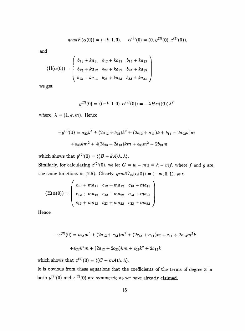
~J(~ ) (o ) = ((B + kt l )X. A). :(?) ( O ) = ((C + mil),\. A ) .

,where X = (1 . Il. rn) is the tangent vector ut the origin.

Proof of proposition 2 . In order to prove this. suppose that the curve cr<c,,> (x) =

(x. y (x). z(x)) lies on the surface F = O. Then F ( q k , , , (x)) = O. For simplicity ive

mi te cr in stead of û ( ~ . ~ ) . By differentiating both sides of the eqiiation we get

(gradF(cr(x)) . a' (x)) = O

which implies t hat

where

This expression holds for any surface F containing the g a p h of the curve U(X)? in

particular for F = u - ku = g - k f . where. f and g are the sanie functions in (2.5).

Since

y ' 2 ' ( ~ ) = ( ( - k . 1.0). ûe)(0)) = -,\HÛ((o))x'

where. A = (1. k. in). Hence

which shows that y ( 2 ) ( 0 ) = ( (B + ICA),\. A ) .

Similarly. for caiculating 2") (O) . we let G = - mu = h - rn f. where f and g are

the same functions in (2.5). Clearly. gradG,(a(O)) = ( -m. O. 1). and

+a22 k2m + (2ai2 + 2c23) km + q2k2 + 2ct2k

which shows t hat -(*)(O) = ((C + mA),\. A ) .

It is obvious from these equations that the coefficients of the terms of d e g e e 3 in

both Y ( ~ ) ( o ) and ~ ( ~ ~ ( 0 ) are sjmmetric as w e have already clairned.

Remark 1. These propositions can be easily extended t o arbitrary dimensions. but

we d o n t need to do this.

Our niain result in this section is the Following.

Theorem 2: 54circles theorem. Consider a sirnple bundle of circles passing

through the origin such that the set of tangent lines o j the circles contams a 54

generic lines. then there ens t s a local diffeomorphism about the o n g m mapping al[

the circles into struight lines if and only if al1 the circles rn the bundle pass through

one common point distinct from the ongin.

Proof. In one direction the proof is obvious. In fact. if the bundle passes through

the second point Q. t hen we can make an inversion with respect to a sphere centered

at t his point. But in the opposite direction. the theorem is rat her cornplicuted and

the proof is the following.

The equation for a simple bundle of circles with center a t (O. O. 0) has the following

form:

where. -4 = 4 k . m ) and B = B ( k . m) are some functions of the parameters k and

m. We show that the rectifiability of the bundle is equiwdent to the linearity of the

Functions A and B. \Lk wish to solve the equations for the circles in the bundle

up to terms of fourth order of smdlness. so by differentiating both equations with

respect to x for the Taylor series of y (x) and ~ ( x ) we obtain

4s) = mx + c2(k. m)x2 + u3(k m)x3 + &4(k. m)x4 + . . . a-here. by letting f = 1 + k2 + m2. we have

where 01 and are polynomials of degrees at rnost 21 - 1 in the two variables k and

m (proposition 1). and -4. B are. at the outset. just rational functions in k and m.

Lire want to show that -4 and B are polynomials of degree 1.

hlultiplyirig equat ions (2.8) by f yields

According to proposition 1. the functions (02, u3). (0s. us) and (O+ ul) are 2-tariable

polynomials of degee at most 3.5. and 7 in k. m respectively. Equations (2.10) are

satisfied for al1 values of (1. k. m) corresponding to circles in the bundle. Le.. by

at least a 54 directional vectors corresponding to 54 generic iines. According to

what we proved in Appendix 2. '-variable polynomials of degree 5 %-hich coincide at

54 direct ional vectors. coincide ident ically. so t hese equat ions are in fact ident it ies.

These identities irnpIy either: f divides (k& + m th). or: 1 divides both o2 and G2.

In the latter case equations (2.7) show that -4 and B are polynomials of degree 2.

So we may assume that f g = X'Q + rn ,vy2 for some polynomial g.

fg = k& + rnc2

= k A f + m B j (by equation (3.7))

= ( k A + mB)f

Thus kA + mB = g is a polynomial.

hluitiplying equations (2.9) by f yields

By the same reasoniiig as before. these equations are again identities. This shows

t hat eit her: / divides ( 0 3 + w i ) . or: J divides bot h 0 2 and 0. In the second case.

as before. ive are done. so we niay assume tliat /I(of + uf). Equation (2.8) give

so / ( m o 3 + ku3) = 2krn(of + w i ) + 2(k2 + m2)ec i?

Since we already know t hat /I (4 + ui) it FOUOIVS t hat f 102 c-. Thus ive also have

fl(q2 f &)? and thus fi& it cz and finally f!02 and flv?.

Since these polynomials are polynornials of degree 3 in k and m. .4(k m) and

B(k. rn) would be polynomials of degree 1. in k and rn .Le..

By using the symmetric relations in proposition 2 we see that b = cl = O and a = e.

Hence the fimctions -4 and B are in the form

These linear functions show that our rectifiabLe bundle of circles necessarily has the

form

where. Si = O. S2 = O and S3 = O are the eqiiations for certain non-tùngent spheres

pwsing througii tlie poiiit (0.0, O). We deiiute by Q tlie aecuiid point <jf iiitersectioii

of the spheres SI = O. S2 = O and S3 = O. All the circles in the bunclle pass tlirough

Q. In order to rectify such a bundle of circles. it suffices to take the point Q to

infinity via a conforma1 transformation. S o w the proof of theoreni 3 is complete.

2.2 Rectification of a Bundle of Spheres in Rn

In this section. we deal with the rectification of a bundle of spheres. To be more

precise, we shall concern two different types of spheres: the spheres of codirnension

1 and codimension 2 in Rn. As we shall see. everything is similar to that of circles

in R3 except that our discussion here is multi-dimensional. Let us first $ive some

definit ions and notations.

Rectifiable bundle of hypersurfaces. A bundle of surfaces in (n+ 1)-dimensional

space Rn+[ is said to be locally rectifiable if there is a local diffeornorphisni of the

space mapping each surface in the bundle to a segment of a hyperspace. By a bundle

of surfaces at a point p we mean an arbitrary collection of surfaces each of wliich

pass through p. As in the case of circles we cal1 t his point tlie center of the bundle

and the bundle itself is caUed a central bundle. A bundle is called simple if different

surfaces of the bundle have ditferent tangent spaces.

If a bundle of surfaces is locdiy rectifiable near the center of the bundle. t hen it is

simple. We are interested in the behavior of the surfaces in a rectifiable bundle near

the center. The h-vpersurfaces F,(x. y) = (x. y(x)). whereF,(O) = 0. v F ( 0 ) = cr =

(al, .... a,. 1) and x = (xl. .... 1,). with (x. y) E Pt' will be regarded as the graphs

of the surfaces passing through the origin. Bearing this notation in mind. we have

the following proposition:

Proposition 3. Suppose that a simple bundle of hypersurfaces Fa (x, y ) = (x. y(x))

svbject to the condition F,(O) = O . v F ( 0 ) = cr is locally rectifiable near the origin by

means of a Cm d~ffeomorphisrn. Then for euery r . 1 5 i 5 m. there erist n-rariable

polynomials P&-, . ( j = 1. .... n) of drgree at most (32 - 1 ) such that

For the proof as in the case of the circles. ive need a simple lenima whicli is an

immediate consequence of the implicit funct ion t heorem.

Lemma 2. Suppose that there exists a Cm function G : Rnil - R such that

Let

G(ri . .... x,. 9 ) = 1 a,, .... pn+, zT1 . . . ~ p y ~ ~ - ~ y(z) = bpi +,$ ... ir be the Taylor polynornials for the function G and y respectiriely such that

Then the coeficients bP,..,, is equal to some n-uoriable polyno~mials of degree (2i - 1 )

in the coeficiats a, ,...,,,, .

Proof of lemma 2. By the implicit hnction theorem. the equation

can be solved locally for the function y(x) and this function is a smooth function of

class Cm. in fact we have

Similarly by differentiating the above equation with respect to x, , we get

Solving these equations for y,,, a t the origin we obtain the desired polynoniials

for i = 2. Continiiing in t his fashion. we can consecutively get dl of the ot hcr

polynomials.

Proof of proposition 3. Consider a diffeoniorpliism Q rectifjping the bundle of

hypersurfaces F,(x). Let T be an arbitrary non-singular linear mapping of the

space. The diffeomorphism T o @ also rectifies the bundle Fa. By a siiitabIe choice

of T we can arrange that the rectifying diffeomorphisni has the identity differential

at the point O. The rectifying diffeomorphism is now given by

where

ft(.r) = x* + ... . l S 15 TL,

where . . . denotes the higher order terms.

In the (u . . . . un+ I ) space the bundle of surfaces Fa (x) is given by the eqirat ion

Consequent ly. the surfaces Fa (x) are given by the equat ion G, (1) = 0.

tvhere

Xow the coefficients a,, -.,,+, in the Taylor polynomials of the surfaces Ga depend

linearly on cr = (ai. . . . . a,. 1). Proposition now foliows From lemma 2.

Having proved the above proposition. ive are now ready to state the fundamental

theorem of rectification for the spheres of codimension 1 in Rn+'.

Theorem 3. Consider a rich bundle of sppheres i n Rnil passirtg through the origrn.

then there ezists a local difleoreornoiphism ubout the origin rnapping al1 the spheres into

hyperspaces if and on23 (/ al1 the spheres pass through one cornmon point distinct

fi-am the origin.

First Proof. The equations for a bundle of spheres with center at O can be easily

reduced to the form < a , x >= A < x . x >. where a = (m. .... a,. 1) and x =

(xl, .... r,+l). and A = A(a) is some function of the paranieters ai. .... a,. As in

the 3-dimerisional case of the circles. we show that the rectifiability of t his bundles

is equivalent to the linearity of the Function A. To do this ive consider the l u t

variable x n + ~ as a irnplicit functioii of the reniaining lariables. By differentiating

this variable partially with respect to any other independent variable ive get

where.

a x n + 1 ai = -- d~ (0)

Substituting 2.4 from the first equation into the second yields

By proposition 3 the functions

are n-vaciable polynomial functions of degree at most 5 and 3 in al. .... a, respec-

tively The last equat ion holds for all values of (ail : . . .. û,. 1) corresponding to spheres

in the bundle, i.e.. at l e s t for a generic !V-tuple of spheres. Since n-variable polyno-

mials of degree d which coincide at a generic N-tuple of spheres coincide identically.

d2rn (0). the above equation is in fact an identity. This implies that (1 + af) divides

Since the latter is a polynornial of degree at most three. it follorvs that A(&) is a

linear function of a. i.e..A(aj =< a.cr >. rvhere cl = (ui. .... u n i l ) is a cu~ i& iu t

vector in Rn-'. Thus the equation for a rectifiable bundle of spheres has the form:

This is equivalent to the systeni: x, = a, < r. x >. i = 1. .... n -+ 1. Mk see that ali

the spheres in the bundle passes through the single point

( ai ).i = 1 ..... n f l .

< a.a > Conversely, if the bundle pass through one point distinct from the center of the

bundle, then by making an inversion with respect to a sphere centered at the second

point. ive can easily map the bundle into hyperspaces.

Second proof. By the first proof. it is enough to prove the theoreni only in one

direction. This proof is absolutely independent of the fist proof and is given by

induction on n for a bundle containing at least rz + 5 spheres in Rn. Having said

that. we can now restate our theorem as: suppose that a bundle of spheres passing

throiigh the origin and containing at least n + 5 . (2 5 n ) spheres in Rn is locally

rectifiable. then al1 the spheres pass through one point distinct from the previous

one. For n = 2, this is just the 2-dimensional rectification problems of circles. For

n = 3 we have at least eight z-dimensional spheres al1 of which lie in R3. Fis one

sphere and take the intersection of the remaining spheres with the first. Let S be the

stereographic projection which send this fived sphere into a plane. If T is the desired

rectifying map, then the composition map T o S-' is a rnap rvhich send a bundie

of circles in a plane -the image of circles on the fked sphere under stereographic

projection- into straight lines. Since this bundle contains at l e s t T circles. by the

Sdimensional result it shodd pass through a second common point p distinct fiom

the point S(0). It follows t hat d l circles on the fked sphere and consequently al1

the spheres pass through which is distinct From the origin. Sow suppose

that the staternent is true for n = k . We will prove that it is true for n = k + 1. So

suppose that a collection of k-dimensional splieres pusing through the origin and

containing at least (k + 1) + 5 splieres iil R"" is iocally rrctifialle. tlieii aj aLuvr

we fbc one sphere and takc the intersection of this sphere with the reniaining ones.

Clearly the new collection will be a collection of (k - 1)-dimensional spheres which

contains at least (k + 5) spheres. By induction. this collection pass through another

point distinct from the origin. It follows that the main collection also pass through

this second point. The proof is complete.

Xext theorem shows that the same resiilt holds for the spheres of codiniension

2 in Rn. However there is a little difference between this and the previous case.

Since t here is a possibility of empty intersection arnong the ?-dimensional spheres

of &dimensional space f?. we will discuss this case separately and will apply the

induction proof for n = no + 4. where no is a positive integer.

Theorem 4. Conszder a rîch b,undle of spheres of codimension 2 in Rn passing

through the ongin. then there exists a local diffeomo~hism abod the ongin mapping

al1 the spheres into hyperspaces of the same dimension if and only if al1 the spheres

pass through one common point distinct from the origin.

Proof. First suppose tliat n = 4. In this case the bundle consists of 2-diniensional

spheres. Xow the equation for a simple bundle of spheres with center at (O. 0.0.0)

has the form a(+. y) = (x. y, r(x. y).t(x. y)) . where

z = k x + m y + A(xL +tj2 + r2+ t') t = nx + l y + B(x2 + + z2 + t 2 )

and. A = A(k. m. n. I ) and B = B(k. m. n. 2 ) are some rational functions of the

parameters k. m. rt: and 1. We show that the rectifiability of the bundle is equivalent

to the linearity of the functions il and B as welI as some relations among the

constant coefficients of these functions. Using the same argument as the proof of

theorem 2 for the partial derivatives of the hnctions :. t with respect to the variables

x, y we can easily show that the funct ions A. B are in fact linear funct ions of the

parameters ment ioned above. Siniilarly to find the symniet ric relations suppose

that the sphere n ( r . y j = jr. y, z j r . yj. tjr. y j j lies oii clle followiiig two 3-Fuida F =

u3 - kul - mu-. G = u, - nul - lu?.

where ui = j , ( x . y. i. t ) i = 1. .... 4 are the component Functions of rectifying dif-

feomorphism. By partial different iat ion of t hese equat ions Ive get

which imply that

It follows t hat t here exist four 4 x 4 symmet ric matrices -4. B. C. and D such t hat

y,,(O)=((C+kA+rnB)o.r) ~ , , (O)=( (D+nA+lB)u~ .w) .

where. L' = (1.0. k. n) and (L' = (O. 1. m. 1). This relations imply that

A = a k + h + c . B =an+bZ+d.

We see that the equation of our bundle reduces to the following form:

where, Si = 0. S2 = O, S3 = O and S4 = O are the equations for certain non-tangent

spheres passing through the point (0.0.0.0) in p. Lire denote by Q the second

point of intersection of the spheres SI = 0. S2 = O. S3 and S4 = O. Al1 the spheres

in the bundle pass t hrougli Q. In order to rect ifv such a bundle it sufices to take

the point Q to infinity via a conforma1 transformation. The proof for n = 4 is now

complete.

Next suppose that n = na + 1 aliere no is a non-negative integer. As we did

before. the proof for this part is given by induction on n for a bundle of splieres of

codimension 2 containing at least n + 50 spheres in Rn. For n = 5 . this is just the

bdimensional rectification problem For circles. Since by fixing one spliere and taking

the intersectioii of this fked sphere with the others we get a rectifiable bundle of at

least 54 circles in R3. Let S be the stereographic projection which send this h e d

sphere into the space R3. If T is the desircd rectifying map. then the composition

map ToS-' is a map nhich send a bundle of circles in the space R3 (i.e.. the image of

circles on the fised sphere under stereographic projection) int O straiglit lines. Since

this bundle contains at least 54 circles. by the bdimensional result it should pass

through a second point p distinct from the point S(0). I t follows t hat al1 the circles

on the h e d sphere and consequently al1 the spheres p a s t hrougli S-' (p) rvhich is

distinct from the origin. Non- suppose that the statement holcIs for n = k . IR will

prove that it holds For n = k + 1. So suppose that a collection of k - 1-dimensional

spheres passing through the origin and containing at l e s t k + 1 + 50 spheres in R'"

is locally rectiçiable. t hen we fi'c one sphere and take the intersection of this sphere

with the remaining ones. Clearly the new collection will be a collection of (k - 2)-

dimensional splleres which contains at least ( k + 50) spheres in Rk By induction.

this collection pass through another point distinct from the origin. It follows that

the main collection also pass through the same point. The proof is complete.

Chapter 3

Classification Theorems

Consider the space S of equations of spheres in Rn. i.e.. the space of non-zero poly-

nomials of the form

Clearly. every element of this forni is defined up to a factor. Tlius the space V

is isomorphic to the projective space RPn". A projective subspace L of V of

dimension k(k = 1. ... . n) is called a k-dimensional linear systern of spheres. Amoug

al1 dBerent linear systems. there are t hree systems which are closely related to the

three geometries of Lobachevski. Euclid. and Riemann : the linear systeni of al1

spheres orthogonal. respectively to a Lsed sphere of positive radius: xy=l 1: = 1.

zero radius: x:=L xf = 0. and imaginary radius: x:= x: = - 1 . These t hree

different linear systems can be defined as:

Definition 1. A n-dimensional net of spheres is any set of spheres. the equations

of which Lie in some n-dimensional iinear system but not in a q ( n - 1)-dimensional

linear system.

Definition 2. Characteristic map. A characteristic rnap of n-dimensional net is a

map @ : Rn - R F

defined by

+(-Y) = isl(.Yj : s2(Xj : ... : snT1{Xji

where. SI. sz. ... . and s, ,~ are any ( n + 1) independent quadratic polynoniials in the

space V . h characteristic niap @ depends on the choice of the polynomials s, and

is t herefore defined up to a projective transformation.

Definition 3. Degeiierate point. The point (xl. .. .. r,) of a characteristic map <P.

rvill be called a degenerate point of n dimensional net of spheres if @ has the zero

Jacobian at t hat point. The degenerate points of the t hree linear systems of spheres

indicated above consists. re~pectively. of the points on the sphere Er=, x: = 1. the

point (0. .... 0). and the empty set.

3.1 Rich Families of Circles in R~

Definition 4. Suppose that A is a faniily of circles in some domain U. It is called

a rich family. if there exists a sub-family r Ç h such that

(1). For each p E Ci t here existu a circle E r such that p E 7.

(2). If 7 E r and p E -,, then t here exists an open cone hPp -1t is assumed t hat the

cone depends continuously on the point p such that the tangent Line of 7 ac the

point p lies inside h',. and any other direction in Kp corresponds to a circle in T.

Next two theorems give complete description of all local diffeomorphisms which

rectify a rich family of circles in some domain Li.

Theorem 5. A rich family O/ circles in R3 in a neighborhood O/ the point p is

rectzfiable if and only zf there exists a g e r m of a dzffeomorphism

yzven by

where

with a non-zero Jacobian such that eoery circle in the familg is the incerse image of

a line under a. To prove this theorem. we need some simple facts which Ive state as the followiiig

two lemmas.

Lemma 1. Suppose that S is a sphere wrth center at O and radius r . Suppose Q rs

the inversion poznt of P wzth respect to S . i.e.. the points O. P. and Q are colinear --

and we have O P a OQ = r2. then any circle passing throvgh the points P and Q is

orthogonal to S . Conversely if c is a circle which is orthogonal to S . then for any

line L passing through O such that L n c = {P.Q} . P.Q are inuersron points with

respect to the sphere S .

Proof of lemma 1. Suppose that c is any circle passing through the points P and --

Q with T E S n c. then the number OP-OQ is the potver of the point O with respect -- -

to the circle c. Xow the relation O P OQ = r2 = 0T2 shows that OT is tangent

to the chde c at the point S. Thus c is orthogonal to S. The converse assertion

is immediately foliows by definit ion and the propert ies of the power of a point with

respect to a circle.

Lemma 2. Let S be the same sphere S in lemma 1. Let ci and cz are tmo orthogonal

circles to S such that cl n c2 = {P. Q } . Then the principal axïs of cl and c2 (i. e. .

the line joining the two cornmon points of the circles) passes through the point O. P. --

and Q and we have O P a OQ = r2.

Proof of lemma 2. The second assertion follows immediately from the converse

statement of lemma 1 after proving the first one. First assertion follows by rnapping

the sphere S ont0 a plane II via an inversion map. Since both circles cl and c?

are orthogonal to Ii. then it is the piane of syrnmetry such that P and Q are

symmetricd points with respect eo it. Clearly the line passing throiigh these two

points is perpendicular to ll. By taking the inverse images. cile origirlal l i m is

perpendiciilar to the sphere S. Yow a e are ready to prove theoreni 1.

Proof of theorem 5. Let us first suppose that the rich family of circles is rectifiable.

Let c = O be the equation for some circle iri the faniily passing througli the point

P. with a tangent lying inside the cone Kp. Let .4 and B be two points on the

circle c = O lying close to P but on different sides. The circles in the farnily passing

through the points .4 and B form rectifiable btindles by our assitmption. Hence by

theorem 2 of chapter 2. they pass through the points C and D respectively distinct

from A and B. Through each point Q close to the P. (Le.. Q contained in both K..,

and K B ) , there exist circles in the family of circles passing through the points A. C

and in the family of circles passing through the points B. D. Again by theorem 2

al1 circles in the family passing t hrough the point Q pass a single point R distinct -

from the point Q. Now suppose that the lines containing the segments and BD

intersect a t some point O. By definition of the power of the point O with respect -- -- -- --

to the circle c, ive have 0.4 OC = OB . OD. Let r' = 0.4 OC' = OB . OD and S

be the sphere with center at O and radius r. We wi1I show that the two points Q

and R are inversion points with respect to the sphere S- First of ail. by lemma 1.

we see that A and B are respectively the inversion points of C and D with respect

t o the sphere S. This shows that all circles passing through the points .4. C and B.

D are orthogonal to S. Secondly, by the above rernarks. there p a s circles cl and

cz in the families of circles passing t hrough A. C and B, D and bot h f a d e s are

orthogonal to the sphere S. then by lemma 2. the line passing through the points Q --

and R passes through the point O too, and we have OQ a OR = f2. This shows that

Q and R are inversion points with respect to the sphere S. and al1 circles passing

t hrough t hese two points are orthogonal to the spher2 S. According to the different

positions of the point O! vie have the following different cases.

Case (1). The point O lies outside c. In this case. we rnap the sphere S ont0 the

unit sphere with ceilter at the origin via a spherical transformation ( a conforma1

trÿnsformatiori wliicii iiiaps every çirçle tu a circle alid every apliera t u a spliere).

In fact. by using only a dilation followed by a translation. Since these two motions

are conformal niappings and they map circles into circles and spheres into spheres.

we see that any orthogonal farnily of circles on S will automatically be mapped into

an orthogonal farnily of circles on unit sphere centered a t the origin. By tliinking of

an orthogonal circle as an intersection of two orthogonal spheres. ive can write the

equations of the farnily of circles as a pair Si = O. S2 = O where. SI and S2 are the

equations of the spheres of the form

with different parameters a. b. c. By taking the homogeneous form of t hese equations

with respect to the coefficients a. b. c. i.e..

-42 + By + Cz + D(r2 + y' + 2' - 1) = 0.

we can w ~ i t e down the characteristic map as

9 3 $(x.y. zf = [x: y: : : 1 - x' -y- - z-1.

Case (2)). The point O is on the circle c. In this case. the sphere S is just a

single point O. In other words. we have a sphere of radius zero. By mapping this

single point to the origin. we see that all the circles or equivalently. al1 the spheres

orthogonal to this sphere are of the form

or by using an inversion ive get as + by + e + 1 = O which in turn gives rise to the

hornogeneous form: Ar + By + Cs + D = O. In this case. the characteristic rnap is

@(..y.-) = [r : y : 2 : Il.

Case (3). The point O lies inside c. In this case. the sphere S is an iniaginary

sphere. By mapping this sphere onto the imagina- unit sphere at the origin. Le..

rZ + + :' = - 1 for the equations of orthogonal faniily of spliere S we have

or equivalentk. for the hornogeneous form we get

Thus the characteristic map for this case is

To complete the proof ive only need to show that for each rich family of rectifiable

circles the characteristic map is the same from one point to another. To prove t his

last assertion. suppose that P. Q E LT such that P # Q. Since any curve joining

the t1i-o points P and Q is a h i t e curve or a segment. w can cover t his curve by

a finite nurnber of bdls such that the center of each bal1 lies in the nelT. Each

characteristic map is a analytic function and a- two characteristic maps coincide

in the intersection of their domain. so they coincide identically by the theorem of

analyt ic continuation.

Thus the equations for all the circles in our rectifiable family lie in tn70 different

linear combinat ions of the equations Si = O. S2 = O. S3 = O and S4 = O. Sloreover.

we can easily see that near a nondegenerate point of a rich funily there does not

exist a q rectifiable rich subfamily (this can be verified separately for the three h e a r

systems of circles). Near a nondegenerate point of the family, the family is rectified

by the chuacterist ic transformation

where

I t remains to show that up to a projective transformations there esist no other

rectibing maps. This is an inmediate consequence of lemma 3.

Lemma 3. .4 local diffeomorphism of the space which takes a rich family 01 lines into lines is a projective transformation.

Proof of Lemma 3. It is well-known that a home~morphisnl which sends all lines

into lincs is a projective transformation. The proof of this fact based on constructing

an everywhere Mobius fiat net [i].

To this end. suppose that four lines l,(i = 1. ... .4) in a plane n are in general position.

Suppose F is a map which sends these four lines into another four lines F( l , ) ( i =

1, .... 4) in general position. Sow for any projective transformation T. T(l,)(i =

1. ... , 4 ) are also in general position. Then there exists a projective transformation I/

such that U maps T(1,) into F(1,). So without loss of generality. we may assume that

T(1,) = F(1,) = m,, ( i = 1. .... 4). Suppose that -4. B. C. D. and a. b. c. d. are four

vertices of the quadrilateral formed respectively by I, and rn, . (i = 1. .... 4). Since

both maps F and T map the diagonals of the first quadrilateral to the diagonals of

the second one. It follows that F ( P ) = T ( p ) . where p and F ( p ) are the intersection

points of the pairs of the diagonals respectively.

Continuing in this way. we get a countable dense subset of some neighborhood such

that F = T on this subset. Since both F and T are continuous. we have F = T

on this neighborhood. Xow the proof of lemma 3 based on the same arowent .

If P is a point in the neighborhood U. then we apply the same reasoning for any

plane II passing through the point P. First of all. we can map any four lines in

general position into a parallelogram via a projective transformation. Secondly. by

definition of a rich faniily of lines for any point a E U. there exists a line 1 passing

though the point a. Since a E L. there exists a cone hi such that 1 lies inside

Ka. For a.ny other point b E 1. there esists mother cone 1Cb sucIl t h Z lies i l i d e

Kb. NOW we can easily construct a parallelograni such that a11 four sides as well as

its diameters contained in our rich faniily. Firially. we construct a Mobius put net

inside tliis parallelogram. al1 of whose lines lie in the rich faniily. This implies tliat

the rnapping F is locally projective. The connectedness of the region U now implies

that F is projective. We proved t hat

Theorem 6. Up to a projecticre transformation of the space of the image and a

conforma1 transformation of the space of the inuerse image. there e n s t exactly three

local difeomorphis.tns which rectify rich families of circles. Theyl are given 69:

(2) @(x. y.:) = [r : y : 2 : 11.

(3) @(r.y.:) = [x: g : 2 : 1 + x 2 f g 2 + $ .

Chapter 4

Applications in Riemannian

Geometry

As is well-known. there are three ciassical geometries in which the geodesics in

some local coordinate systeni are straight lines. Beltrami's theorem together with

the Minding-Riemann theorem both of which are n-dimensional results ensure that

t hese geometries are the oniy ones with t hese propert ies. Takinp rz = 3. rite will show

that there are precisely t hree classical geometries wit h geodesics as circles. This is of

course a consequence of the 3-dimensional extension of the Beltrami theorem which

we are going to prove by replacing straight lines with circles. Hon-ever. this result

d k e the previous statement does not hold in arbitraru dimensions. In fact. we will

see that there is a very natural metric in R' with geodesics as circles. but it does

not coincide wit h the t hree classical geometries obtained in the 3-dimensional case

-the metric does not have constant cmzture. We will also point out some remarks

between rectification and Riemannian geornetry which strict- speaking is not an

application but a part of rectification concept which fits best at this point.

4.1 Riemannian Geometry

In this section. first we give a little proof for the bdimensional estension of the

Beltrami theorem. Second. we recall the three rnetrics in which the geodesics are

straight lines. Then in the end. we use these metrics to calculate tlie corresponding

metrics wit h circlc geodesics.

Theorem 1: The 3-dimensional extension of the Beltrami theorem

Up tu a p~ojectioe transformation of the space of the image and u p to a Moboblus

transformation of the space of the inverse image. al1 metncs ln which the geodes-

ics are circles. up to a constant factor. are reduced to the three classzcal examples

mentioned abo ue.

Proof of theorem 1. First of all. note that ail geodesics (circles) passing through

one point is rectifiable bundle by the proposition in section 1.2. Secondly. by theoreni

2 of Chapter 2 any rectifiable bundle in R3 p a s through some other common point

distinct from the center. On the other hand. a11 geodesics in a region U form a rich

family- of circles. Wow by using theorem 5 together rvith theorem 6 of Chapter 3 ive

get the three different characteristic maps.

By theorem 6 of chapter 3. every characteristic map is a geodesic map on Rn(n =

2,3) . The Beltrami theorem now implies that (i has constant cilmature C. Applying

the SIinding-Ricmann theorem ive see that L7 isometric to an ellipt ic spitce if k > 0.

Euclidean if k = 0. and hyperbolic if k < 0.

To have a view of the nature of the metric g in the space of rectifiable families

of circles we first need to draw the attention to some models of geometries in which

the geodesics are straight lines [6].

Remarks. Since our results about the rectification of circles are 2 and 3 dimensional.

the foliowing discussion is only true for n = 2 and n = 3.

Clearly for k = 0. the mode1 is the Euclidean space R" with the corresponding

Riemaanian met ric

ds' = d$ + ... + drn.

Hence by the affine cliaracteristic map a(-) = x we have

For k < 0. we use the gnonionic projection of Dn onto Hn. where

and

Identify Rn with R" x (O) in Rn+l. The gnomonic projection p of ûn ont0 Hn is

defined to be the composition of vertical translation of D" by en, 1 followed by the

radial projection to Hn. An esplicit formula for p is given by

where

First we note that the element of hyperbolic arc length of Hn is

Let u = (1- ly12)-'12. For i = l . . . . ,n me have q = yiu and Z,+I = u. So for

i = 1, .... n. dzi = dyiu + yi(y-dy)~3. and d ~ , , ~ = ( I J . ~ Y ) ~ L . ~ . where g.dy denotes the

standard inner product hetween y = (y l . .... y,) and dy=(dyl. ... . dg,). Thus

For k > O, we sirnilarly use the gnomonic projection of Rn onto Sn, the unit sphere.

To do this.we identik Rn vit11 Rn x {O) in Rn+' . Then the gnomonic projection

is defined to be the composition of the vertical translation of Rn by e,,+l followed

by the radial projection to Sn. An explicit formula for v is given by

where 1 y + enTl 1 is the Euclidean nomi of y + e , , , ~ . Since the element of spherical

arc length of Sn is the element of Euclidean arc length of Rn+ restricted to Su. So

the arc length ds of Sn is given by

n t L ds' = d::.

t= 1

Let v = Jy +e,,J1 i = l . . . . .n? and-,+, = v . Byusingthegnomonicprojection.

we have

This gives us an elliptic mode1 in which al1 geodesics are straight lines in Rn.

Now we are ready to calculate the Riemannian metrics of' these three geometries

in which the geodesics at every point are circies.

Cleariy for k = O this is the standard metric

For the hyperbolic case, we set k = -1. and use the &ne characteristic niap

: R" + Rn defined by

Let w = (1 + lx12)-! Then yi = x, W. and dg, = ds, cl. - 2 x , ( r . d ~ ) up' i = 1. .... n.

Substituting these expressions into hyperbolic metric with geodesics as straight Lines

namely in (4.1) we get the following metric with geodesics as circles.

Finally for the elliptic case we set k = 1. and we use the affine characteristic

map @ : Rn - Rn defined by

x @(x) = = y.

1 - 1x12 Let t = (1 - Ixl2)-!

Then yi = x i t . anddyi = d x 1 t + 2 ~ , ( x . d x ) t 2 i = 1 ..... n. Substitut ing t hese expressions into eilipt ic metric ni t h geodesics as st raigtit lines

namely in (4.2) we get the foilowing metric with geodesics as circles.

4.2 Rectification and Riemannian Geometry

The farnily of al1 geodesics passing through one point on a Riemannian manifold

is alniays locally rectifiable by using the exponential rnap which takes the tangent

space to the manifold in such a way that al1 lines passing through one point become

geodesics. Conversely one can easily prove the following proposition.

Proposition. -4 simple bwtdle of curves in Rn pussing thrmgh a point p is locally

rectijiable if there exists a metric for which all the cvrves becorne geodesics.

Proof. Let @ be the rectifying diffeomorphism. Then for the Euclidean metric g.

9'g is the desired metric.

We close this section with one l u t remark which gives ii necessary and sufficient

condition between rectification and Riemannian geonietry in the ?-dimensional case.

Remark. Let us fix a nietric g in a doniain (; in R2. Let R be a faniily of al1

geodesics with respect to the metric g. Since t his farnily depends on two parameters.

we assume that it is written in the form F ( r . y: u. L') = O. Let us now regard x and

y as parameters and IL and v as variables. LVhen the iisual solvability conditions are

sat isfied. t his equation dcfines our two parame ters family of geodcsic by g = y (x: u. c)

in the (x, y) plane and its dual family v = ~ ( u : x. y) in the (u. c ) plane. Then the

dual family is also a family of geodesics with respect to some Riernannian metric h

if and only if both rnetrics g and h have constant cmatures . This statement is j tist

a reformulation of a main result in 2-dimensionai rectification problems [A].

Proof. Since both families are geodesic with corresponding metrics g and h. it

follows that they both satisfy the differential eqiiations y" = L(s. y: y') and c ' =

:\a!(-u. c: v' ) respect ively. where L. A! me cubic polynomials of y' and ut respectively.

These two conditions are sufficient for rectifiability of both families [dl. Theorem

1 now implies that both metrics have constant curvature. Conversely if they have

constant curvature. by the Minding t heoreni bot h are reduced to one of the classical

models which implies t hat the dual farnily is also a family of geodesics.

Appendix A

Preliminary Concepts

A. 1 Finite Difference Calculus

We start out with some facts from finite ciifference calculus which is usefiil in the

proof of a proposition in the ne.* section.

Definition 1. A function f : G - R defined on a commutative semigroiip G

with the zero element is said to be a polynomial of degree at most k if for any given

elements a 1. . . . . a, of the semigoup G. the funct ion

of the nonnegat ive integers r 1. . . . . x, is a polynomial of degree at most k.

We shall need the classical Taylor formula in finite differences for functions on

a lattice. To each element a E G. we assign two operators on the space of real

functions with domain G: the shiJt operator La defined by the formula

L,f(x) = f (x + a ) . x E G.

and the Jinite diflerence operator D, given by the formula

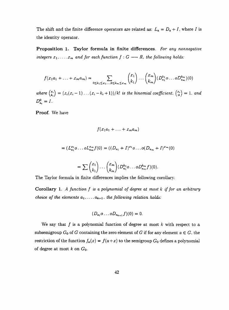
The shift and the finite difference operators are related as: La = Da + I . where I is

the ident ity operator.

Proposition 1. Taylor formula in finite differences. For an y nonnegatiue

mtegers XI.. . . . x, and for each function f : G - R. the folloluing holds:

urhere (;:) = ( r i ( x i - 1) . . . ( r i - k, + l ) ) / k ! is the binomial coeficient. (0) = 1 . and

D:, = I .

Proof. We have

= (L0:o . . . OL;; f ( O ) = ((D,, + I )=lo . . . o(Dam + I ) x m ( O )

The Taylor formula in finite differences implies the following corollary.

Corollary 1. .4 function f is a polynomial o f degrec at most k zf for an arbitrary

choice of the elernents al.. . . .ak+l. the jollowing relation holàs:

We Say that f is a polynomial hinction of degree at most k Mth respect to a

subsemigroup Go of G containing the zero element of G if for aqv element a E G. the

restriction of the function fa (x) = f (a +x) to the semigoup Go defines a polynomial

of degree at most k on Go.

Proposition 2. Let f be a polynomial function of degree at most k with respect to

a subsemigroup Go. Suppose that arnong the elernents al. . . . . a, of G. at least k + 1

elernents belong to the sernigroup Go. Then we have Damo. . . oDa, f G 0.

Proof. Let us enumerate the elements a i . . . . . a , so t hat the first A: + 1 elements

belong to the semigroup Go. Then we have

The function Da,+, o . . . oD,, vanishes at any point n E G. because the function

fa(.) = f (J + a ) is a polynomial on the seniigroup Go of degree at niost k.

Notation 1. We cal1 the expression x(x - 1) . . . (x - n + 1) in the âbove theorem

the discrete power fiirictiori" and we denote it bu x

previous proposition we get the following result .

Corollary 2. -4ny polynomial function i ( x l . . . . . x,)

"1. Using this notation in the

of n-variable XI.. . . .x, can be

'"". i = 1.. . . . n. k, = 1.. . . .d where. W t t e n as a polynomial function ln t e n s of x,

d = deg( f ) . Conversely any polynomial of this kind can be reduced into a usual

polynomial of the same degree.

A.2 Projective Geometry

We say that 2 points p, = [c,] E Pn are independent if the correspondng vectors rp,

are: equivalently if the span of the points is a subspace of dimension i - 1. Note

that any n + 2 points in Pn are dependent. while n + 1 are dependent if and only

if they Le in a hyperplane. We say that a finite set of points -4 c P is in general

position if no n + 1 or fewer of them are dependent.

Yow given any n-variable polynomial of degree d. t here corresponds its homogeneous

po1ynomia.I of the same degree. Listing al1 the rnonomials of t his polynomial in a

fked order we get the Veronese map @en by:

where

Definition 2. We say that S points p l . . . . . p s E Pn are d-good if there exists

a unique homogeneous cone of degree d containing these points. This is in turn

equivalent that the points

are in general position.

We will show that for any .V = (n2d) - 1. there exists at least one set of points

pi, 1 5 i 5 !V in fn such that a&,). 1 5 i 5 LV are in general position. More

strongly, one can easily pove that

is different frorn zero.

Remark 2. This implies that this set of points form an open subset of whole space

P" proving that the image of the generic points in P" are in general position.

To this end. we use the discrete power functions From the previous section to

define the affine Veronese map as follows:

where x,"=I 2 , = d.

We take the lattice points Pi,.*, = ( i l . ... in) in which O < x;=l i, 5 d with the fol-

lowhg order:

if and only if

ik < j k . or ix; = jk. i k - I < jk+

Corollary 3. Suppose that L = QI. . . . . Qs be the set of all points of the lattice

defined as above with the same ordering. then

is an ( X + 1 ) x ( X + 1 ) upper triangular mat& with non-zero entnes on the main

diagonal. where el is the first standard unit vector in R:'''.

proof. It is enough to calculate the above matr~u using the Veronese map.

The next proposition is a fact which we need in Chapter 3 in connection with

the projective transformation.

Proposition 3. Suppose that T : Rn - Rn be a one-to-one map which presenles

straight lines. Then T zs an aBne trasfonation.

Proof. First of al1 we show that if f : R - R is a one-to-one map such that

f (x + Y) = f (4 + f (y): f (XY) = f (4f (y)-

for all x? y in R. then f (x) = x. for ail x in R. To this end.we first observe that

f (0) = 0' f (1) = 1' / ( r n / n ) = mln. Since the rational aumbers are dense in the

real numbers, by assuming f to be continuous and using the limit theorem s e c m

show that f (x) = x, for d real numbers. However. we prove that the function f is

really continuous. Wote that the positive numbers are squares. Le.. if r is a positive

number, t hen r = rl/' . r'l'. So we have

f ( r ) = f ( r l / ' - r l / 2 ) = ~ ( ~ l / ? ) f ( ~ l / ? ) = [ f ( r l / ? ) ] 2 ,

which is a positive number. it foilows that f ( r ) is a positive number when r is a

pohitive iiu~libtir. Su far. ive have proved tliat !(ni in) = r ~ i , ' r i . aiid f prescrves

positivity. If a > b. then a - b > 0. and ive have f (a - b) > O. or equivalently

f ( a ) > f (b ) . Using t his propcrty one can easily show that f is a continuous function.

Thtis f (x) = .r. for al1 x in R.

Secondly. define LTl ( u ) = T ( P ) - T(0). then U1 has just the same properties as T

such that Ul (O) = O. Set CIl (e,) = c,. In other words. Lri niaps coordinate aves into

some other lines passing through the origin. Since Lii is also one-to-one. these lines

cire linearly independent. Defiiie the linear inap G2 such that

u a < , w,) = Et<, .r,et-

Set g = LTpLr l . clearly g(e t ) = et . This iniplies that g t d e s any coordinate m i s ont0

the same coordinate &.sis. We show that at each coordinate mis it is the identity

map. Suppose L be the two different copies of an arbitrary coordinate a i s . Take

0.1, a. b on the h s t copy and g(0 ) = O. g(l) = 1. g(n) . g (b) on the second one. Using

the fact that the parallel lines will niap into the parallel lines. we can easily show

that g(a + b) = g(a) + g(b) . g(ab) = g ( a ) g ( b ) . It follows that g ( a ) = a for al1 a E L.

Yow. we wish to show by induction that g is identity on OSI' plane. O S Y Z space

and so on. Suppose 2 E R' such that Z = Z + a where x. y lie on S and Y axes

respectively. Since these two axes are mapped ont0 the same axes. and two points X

and Y are fised by the identity automorphism. we deduce that g ( x ) = r . g ( y ) = y.

and finally two lines passing through two points x.;y and parallel to the axes are

mapped onto the lines passing through the points x. y and parallel to the axes. Thus

their intersection is 2. In other words. g(r ) = i for aLI 2 E R2. In the next step.

we consider O X Y Z space on which g maps al1 axes as weil as OXY plane onto

themselves and sends any point t such that 3 = Z + a. where 2 lies on 2-axis

and a lies on O X Y plane. The line passing throuph the point a and parallel to the

2-auis is mapped onto the same copy on the second space. Since the line Z lies on -.+

the O X Y plane. it is mapped ont0 itself. The vector A is paralle1 to 2 and passing

through the point 2. it niust be mapped onto a vector parallel to G? and passing

through the point 2. Clearly this vector mil1 be another copy of 3 in the second

space. Tlius two lines intersect at the sanie point t and lieuce ive have y ( t ) = t .

By induction on n ive can show that g(x) = x for al1 x E Ru. Therefore. g is an

identity transformation. Since g = U2 o Ui . we have Lrl = L!;' O g = L4 which is iri

lact a linear trasformation. But T ( c ) = & ( r ) + T(0) . it folloti-s that T is an affine

trasformation. this cornletes the proof.

A.3 Some Necessary Theorems

We close this Appetidix with the staternent of some well-known theorems which are

useful in proving sonie necessary results in our discussions.

1. Implicit function theorem. Suppose thaf f : Rn x Rm -r Rm is contznousely

differentiable in an open set containing (a . b ) and f (a . b) = O . Let 1L.I be the m x m

m a t e

(D,+J'(a. 6)) . 1 < i. j 5 m.

I ' d e t ( M ) # O. there is an open set .L c Rm containing h . uiith the folioming

propert y:

for each x E A there is a unique g ( s ) E B such that f (x. g(r)) = O . The function

g is dzgerentiable [IO].

2. The Minding-Riemann theorem. Let ( M . g ) be a Riemannian manifold of

dimension n > 2 and let k be a real nurnber. Then the folioun'ng are equiualent.

( 2 ) LW is of constant curvatum k .

(ii) If x E hl, then x has a neighborhood which is isornetnc to an open set on

s o m e S " i f k > O , R " i f k = O , H n i f k < n [ 3 . 5 ] .

Bibliography

[1] A. G. Khovanskü. Rectification of circles: Sib. Mat. Zh.. Il. So -4. 221-226 (1980).

[2] W. R. S harpe. Different i d geometry: Cartan's generalization of Klein's Erlangen

program; Springer-verlag 1997 Sew Yourk Inc.. GhIT So. 166 Th.4.3. p.352.

[3] J. A. Wolf. Spaces of constant curi-ature: 5th Edition. Publish or perish Inc.

1984 Th.2.4.11, p.69.

(41 V. 1. Arnold. Geonietrical uietliods in the theory of ODE: Springer-verlag.

Chap. 1.

[5] SI. P. Do carmo. Differential geometry of curves and surfaces: Prentice-Hall.

Englewood Cliffs. SJ . 1976.

[6] J. G. Ratcliffe. Foundations of hyperbolic manifolds: Spriner-verlag 1994 Sew

Yotuk Inc.. GTM 149. P. 192-197.

[7] F. Klein. Vorlesungen Uber Hohere Geomtrie: Chelsea publishing Company Sew

Yourk 1949.

[8] T. L. Hankins. Blood, dirt. and nomograrns. A particular History of graphs:

Annual meeting of the History of Science! San Diago, California. Sov. 1997.

[9] D. Hilbert, Slat hematical problems: Internat iond congres of Mat hemat ics at

Paris. 1900.(13th problemj.

[IO] M. Spivak. Calculus on manifold: W. A. Benjamin inc.. 1965.

[ll] P. Griffiths J. Harris: Principles of algebraic geometry, Wily 1978.

[12] V. 1. Arnold. Mathematical methods of classical mechanics: Second edition.

Springer-verlag, Yew Yourk Inc.. 1989.