recovery, corrosion analysis, and characteristics of
TRANSCRIPT
Recovery, Corrosion Analysis, and Characteristics of Military Munitions from Ordnance Reef (HI-06)
March 12, 2015
Robert George and Bill Wild Environmental Sciences, Energy, and Environmental Sustainability*,
Space and Naval Warfare Systems Center Pacific, 53475 Strothe Road, San Diego CA 92152
Shengxi Li, Raghu Srinivasan, Ryan Sugamoto, Christopher Carlson, Jeffery Nelson, and Lloyd Hihara
Hawai’i Corrosion Laboratory (HCL)**, Department of Mechanical Engineering University of Hawai’i, 2540 Dole Street, Holmes Hall, Room 302, Honolulu, HI 96822
*[email protected] **hawaiicorrosionlab.org
Approved for Public Release
i
Executive Summary Importance of Corrosion. Large numbers of munitions potentially exist on the seafloor of the world’s oceans, and while there is general knowledge of corrosion processes in seawater for metals that comprise underwater military munitions (UWMM) components, there is little or no understanding of specific corrosion behaviors for munitions, which impacts such important parameters as time to breach for initial munition constituents (MC) release, and time to depletion of MC inside the munition under continued corrosion. Corrosion scenarios include unexploded ordnance (UXO) on ranges; discarded military munitions (DMM) at other sites; conventional and nonconventional munitions; deep and shallow ocean environments; UWMM sites with variation in physico-chemical conditions in water column and sediment; and UWMM under three types of nominal exposure conditions - buried, partially buried, or resting on top of the sediment. The results of this study are broadly applicable, to varying degrees, for multiple types of UWMM under these types of corrosion scenarios. Objective of this Study. The overall objective of this effort was to evaluate corroded underwater military munitions (UWMM) and develop a scientific basis for informing predictive modeling of specific corrosion behaviors of shell casings associated with various classes of UWMM in the marine environment. Previous USN efforts have attempted to address corrosion in a similar manner using empirical evaluation of materials for specific munition casings and applying the results toward model development.1 The results of the UXO Corrosion Prediction Model (UXO-CPM) provided estimates for time to perforation for specific and non-specific ordnance shell casings under the three nominal types of exposure conditions described above. However, it is difficult to apply the predictions except to the class of munitions evaluated empirically in a specific corrosion context, resulting in having to treat other munitions in a more general corrosion context. The UXO-CPM also estimates time to perforation for shell casings under ideal conditions for the lifespan of the ordnance, but does not take into account abrasion or scour, exposure to air during low tides, dents, scratches or other physical damage to the casing, galvanic effects due to adjacent or touching metals, or adverse water or substrate qualities such as high temperature, low pH, high Redox potential, all of which could greatly increase casing corrosion rates. Focus of this Study. Corroded UWMM have been investigated here for purposes of developing a scientific approach for understanding specific corrosion behaviors associated various classes of UWMM in the marine environment. The initial focus has been to characterize corrosion behaviors associated with demilitarized DMM upon recovery from the seafloor after 60+ years. The overall effort was comprised of a field effort and a laboratory effort, both briefly described below. 1 “UXO Corrosion Prediction Model”, B. Sugiyama, W. Wild, R. George; International Corrosion Workshop, Newport News, VA (2010).

ii
Study Approach. Field efforts were focused on leveraging a technology demonstration in 2011 that was focused on recovering demilitarized DMM at the sea disposal site Hawaii 6 (HI-06), known locally as Ordnance Reef, treating the recovered munitions by explosive fill decomposition using the explosives hazard demilitarization system (EHDS), and finally recycling of the resulting empty metal shell casings.2 Photos from the field effort are shown in Figure 1 below. A selection of these empty metal casings were collected prior to the recycling step and brought into the laboratory for subsequent evaluation. All of the munitions corrosion samples were photo-documented prior to down-selection for corrosion evaluation and studies reported here. A subset of the EHDS-treated munitions casings is photo-documented below. Laboratory-based studies were undertaken to evaluate corrosion products and, if present, any calcareous deposits associated with DMM, along with compositional metallographic analysis and morphological analysis of DMM casing materials that include steel and copper. In addition, normal and galvanic corrosion on DMM were evaluated under the following conditions: aerated and deaerated artificial seawater and sodium chloride solutions (abiotic), real seawater (biotic), and in sandy marine sediment collected from the Ordnance Reef recovery site. The technical efforts described in this report seek to a) develop an initial understanding of potential corrosion mechanism(s), and b) identify critical parameters that will enhance prediction capabilities for casing failure that would allow penetration of seawater into the interior of the shell casing.
2 Geoffrey Carton, JC King and Josh Bowers, "Munitions-Related Technology Demonstrations at Ordnance Reef (HI-06), Hawaii," Marine Technology Society Journal, January/February 2012 46:63-82

i
Figure 1. Field effort to collect metal casings from recovered DMM during a 2011 technology demonstration by the US Army at HI-06 (Ordnance Reef). The top three rows of photos illustrate the ROV, shore-based ops center, and barge-based recovery and treatment technologies, and the remaining photos show the recovery and demilitarization process/operations.

ii
Figure 2. Examples of field-collected EHDS-treated munitions casings for corrosion studies. Samples collected and treated at the site were subsequently photo-documented and down-selected for corrosion studies at the Hawai’i Corrosion Laboratory (HCL).
iii
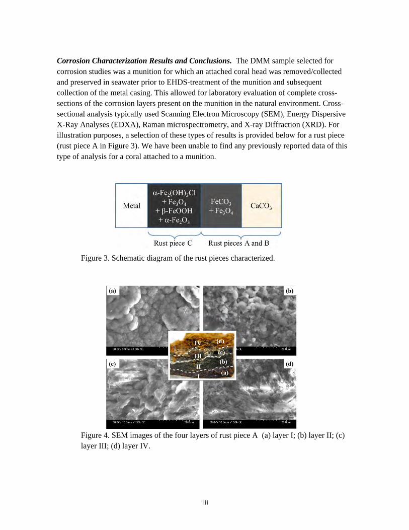
Corrosion Characterization Results and Conclusions. The DMM sample selected for corrosion studies was a munition for which an attached coral head was removed/collected and preserved in seawater prior to EHDS-treatment of the munition and subsequent collection of the metal casing. This allowed for laboratory evaluation of complete cross-sections of the corrosion layers present on the munition in the natural environment. Cross-sectional analysis typically used Scanning Electron Microscopy (SEM), Energy Dispersive X-Ray Analyses (EDXA), Raman microspectrometry, and X-ray Diffraction (XRD). For illustration purposes, a selection of these types of results is provided below for a rust piece (rust piece A in Figure 3). We have been unable to find any previously reported data of this type of analysis for a coral attached to a munition.
Figure 3. Schematic diagram of the rust pieces characterized.
Figure 4. SEM images of the four layers of rust piece A (a) layer I; (b) layer II; (c) layer III; (d) layer IV.
iv
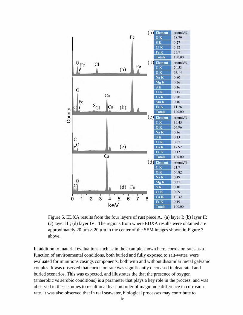
Figure 5. EDXA results from the four layers of rust piece A. (a) layer I; (b) layer II; (c) layer III; (d) layer IV. The regions from where EDXA results were obtained are approximately 20 µm × 20 µm in the center of the SEM images shown in Figure 3 above.
In addition to material evaluations such as in the example shown here, corrosion rates as a function of environmental conditions, both buried and fully exposed to salt-water, were evaluated for munitions casings components, both with and without dissimilar metal galvanic couples. It was observed that corrosion rate was significantly decreased in deaerated and buried scenarios. This was expected, and illustrates the that the presence of oxygen (anaerobic vs aerobic conditions) is a parameter that plays a key role in the process, and was observed in these studies to result in at least an order of magnitude difference in corrosion rate. It was also observed that in real seawater, biological processes may contribute to

v
differences compared to results in laboratory-prepared salt water, and should be considered, particularly if relying on laboratory-derived data and results for corrosion rate estimates. The presence, growth and deposition of corrosion products on the casings in seawater were observed to affect the corrosive process by interfering with galvanic activity for electrically coupled components. The magnitude of the impact on corrosion by such deposits or by biological growth will be dependent on the localized environments in which the munition resides.
Figure 6. Raman spectra from layer I of the rust piece A (a) dark-red region; (b) black region 1; (c) black region 2; (d) white salt crystal.
vi
05
10152025303540455055
rust piece C rust pieces A and B
Concreation layerIntermediate rust layer
Inner rust layer
Ato
mic
%
Position (a.u.)
Fe Cl Ca
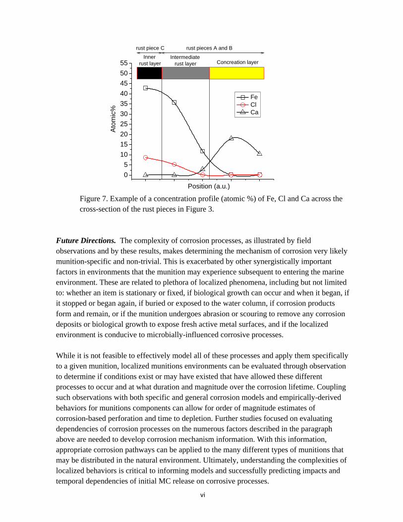
Figure 7. Example of a concentration profile (atomic %) of Fe, Cl and Ca across the cross-section of the rust pieces in Figure 3.
Future Directions. The complexity of corrosion processes, as illustrated by field observations and by these results, makes determining the mechanism of corrosion very likely munition-specific and non-trivial. This is exacerbated by other synergistically important factors in environments that the munition may experience subsequent to entering the marine environment. These are related to plethora of localized phenomena, including but not limited to: whether an item is stationary or fixed, if biological growth can occur and when it began, if it stopped or began again, if buried or exposed to the water column, if corrosion products form and remain, or if the munition undergoes abrasion or scouring to remove any corrosion deposits or biological growth to expose fresh active metal surfaces, and if the localized environment is conducive to microbially-influenced corrosive processes. While it is not feasible to effectively model all of these processes and apply them specifically to a given munition, localized munitions environments can be evaluated through observation to determine if conditions exist or may have existed that have allowed these different processes to occur and at what duration and magnitude over the corrosion lifetime. Coupling such observations with both specific and general corrosion models and empirically-derived behaviors for munitions components can allow for order of magnitude estimates of corrosion-based perforation and time to depletion. Further studies focused on evaluating dependencies of corrosion processes on the numerous factors described in the paragraph above are needed to develop corrosion mechanism information. With this information, appropriate corrosion pathways can be applied to the many different types of munitions that may be distributed in the natural environment. Ultimately, understanding the complexities of localized behaviors is critical to informing models and successfully predicting impacts and temporal dependencies of initial MC release on corrosive processes.

vii
Table of Contents
Executive Summary ..................................................................................................................................... i
1 Introduction .......................................................................................................................................... 8
2 Part 1: Characterization of the Corrosion Products from the Retrieved DMMs Before and After Exposure to the EHDS .......................................................................................................... 12 2.1 Objectives .............................................................................................................................................................. 12 2.2 Experimental ....................................................................................................................................................... 12 2.2.1 Raman Spectroscopy .......................................................................................................................... 12 2.2.2 Scanning Electron Spectroscopy and Energy Dispersive X-‐Ray Analyses ................... 12 2.2.3 X-‐Ray Diffraction ................................................................................................................................. 12
2.3 Results ..................................................................................................................................................................... 13 2.3.1 Raman spectroscopy results ........................................................................................................... 14 2.3.1.1 Corrosion Products from Steel Casing Before Exposure to EHDS ............................................ 14 2.3.1.2 Corrosion Products After Exposure to EHDS .................................................................................... 17 2.3.1.2.1 Corrosion Products on Steel Casing ............................................................................................... 17 2.3.1.2.2 Products on Copper Rotating band ................................................................................................ 18
2.3.2 SEM/EDXA results .............................................................................................................................. 19 2.3.2.1 Corrosion Products from Steel Casing Before Exposure to EHDS ............................................ 19 2.3.2.2 Corrosion Products After Exposure to EHDS .................................................................................... 23
2.3.3 XRD results ............................................................................................................................................. 25 2.3.3.1 Corrosion Products from Steel Casing Before Exposure to EHDS ............................................ 25 2.3.3.2 Corrosion Products After Exposure to EHDS .................................................................................... 26
2.4 Discussion .............................................................................................................................................................. 28 2.5 Conclusion ............................................................................................................................................................. 30 2.6 References ............................................................................................................................................................. 30
3 Part 2: Corrosion Experimentation with DMM Steel Casing and Copper Rotating Band Materials .......................................................................................................................................... 31 3.1 Objective ................................................................................................................................................................ 31 3.2 Background .......................................................................................................................................................... 31 3.3 Experimental Procedure ................................................................................................................................. 34 3.3.1 Material Characterization ................................................................................................................ 34 3.3.2 Polarization Experiments ................................................................................................................ 34 3.3.3 Artificial Seawater ZRA Experiment ............................................................................................ 36 3.3.4 Cell Conditions ...................................................................................................................................... 37 3.3.6 Electrolytes ............................................................................................................................................ 39
3.4 Results and Discussion ..................................................................................................................................... 41 3.4.1 Material Characterization ................................................................................................................ 41 3.4.2 Polarization Experiments ................................................................................................................ 43 3.4.3 Artificial Seawater ZRA Experiments ......................................................................................... 47 3.4.4 Real Seawater ZRA experiments ................................................................................................... 52
3.5 Conclusions ........................................................................................................................................................... 57 3.6 References ............................................................................................................................................................. 57

8
1 Introduction
Department of Defense sea disposal site Hawaii 6 (HI-06), known locally as Ordnance Reef, is a shallow-area fringing reef approximately 4 km x 2 km in size adjacent to the Waianae shoreline on Oahu. HI-06 was used for disposal of discarded military munitions (DMM) after World War II. It is estimated that at HI-06 there are approximately 20 different types of munitions, and over 8000 individual small to large caliber and other munitions3, which are likely to contain high explosives and may also contain propellants that present a potential hazard. A technology demonstration effort at HI-06 was conducted in 20114 to:
1) recover and demilitarize the DMM by degrading explosives and propellants
using the energetic hazard demilitarization system (EHDS), and
2) recycle the empty DMM casings. The recovery of munitions provided a unique opportunity to study DMM casing samples collected between steps 1 & 2 and examine some of the DMM specimens that have been under water at HI-06 for an estimated 60 years or more. To date, relatively little is known about the corrosion behavior and rates of undersea DMM, making it difficult to assess the timeline for and nature of DMM casing breaches due to corrosion, which would lead to the potential release of explosives and propellants into the marine environment. HI-06 is just one of many underwater where munitions are present in the aquatic environment, and corrosion studies of the casings will aid in understanding the mechanisms and release rates of the contents of munitions to the environment. Hence, the goals of this project were to:
1) Characterize the actual corrosion morphology of DMM retrieved from OR, 2) Identify the DMM materials, 3) Conduct corrosion studies on the DMM materials, 4) Compare the actual corrosion morphology of the DMM to that of generated in
the laboratory study, and 5) Use the results to develop a better understanding of DMM corrosion for the
3 Sonia Shjegstad Garcia, Kathryn MacDonald, Eric Heinen De Carlo, Mike L. Over, Tony Reyer, Jason Rolfe, “Discarded Military Munitions Case Study: Ordnance Reef (HI-06), Hawaii, Marine Technology Society Journal, Fall 2009 Volume 43, Number 4.
4 Geoffrey Carton, JC King and Josh Bowers, "Munitions-Related Technology Demonstrations at Ordnance Reef (HI-06), Hawaii," Marine Technology Society Journal, January/February 2012 46:63-82

9
ultimate purpose of gauging the time until initial release of the munitions fill and in ultimately estimating the duration of that release.
A typical Army or Navy artillery shell consists of a steel body and various components as shown below.
! Figure 1.1. Cross-section of typical artillery shells. [Department of the Army,
1950. Artillery Ammunition, Technical Manual 9-1901.] Most of the munitions recovered during the technology demonstration were
encrusted with calcareous deposits from coral growth. Prior to being released for the corrosion study, the recovered munitions were sectioned with a band saw to expose the
10
explosive filler. The sections were placed in trays and heated in radiant/convection batch ovens, called the explosive hazard decomposition system (EHDS) to thermally treat the explosive fill until non-explosive decomposition. The munitions were heated to 170 to 290°C for 60 to 70 minutes depending on the explosive filler. The explosive fillers encountered include Composition B, amatol, and Explosive D. Most of the artillery projectiles recovered were Explosive D filled.
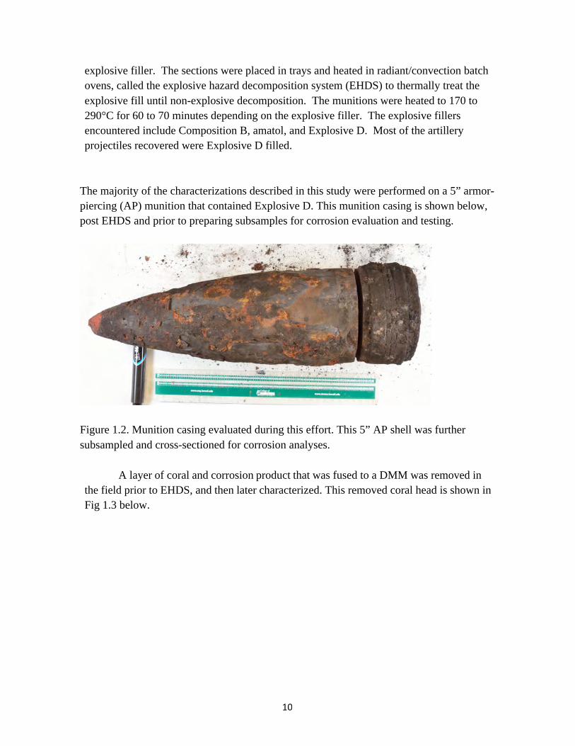
The majority of the characterizations described in this study were performed on a 5” armor-piercing (AP) munition that contained Explosive D. This munition casing is shown below, post EHDS and prior to preparing subsamples for corrosion evaluation and testing.
Figure 1.2. Munition casing evaluated during this effort. This 5” AP shell was further subsampled and cross-sectioned for corrosion analyses.
A layer of coral and corrosion product that was fused to a DMM was removed in the field prior to EHDS, and then later characterized. This removed coral head is shown in Fig 1.3 below.

11
Figure 1.3. Coral head removed from a 5” AP shell.
Corrosion products from the munition casing (steel body) and a thick layer of calcareous deposits that formed on copper rotating bands were also analyzed after being subjected to the EHDS. Scanning electron microscopy (SEM), energy dispersive X-ray analyses (EDXA), X-ray diffraction (XRD), and Raman spectroscopy were used to perform the materials characterization. The munition casing and rotating bands were analyzed using EDXA and optical emission spectroscopy (OES) to determine their elemental compositions. The casing was composed of plain carbon steel (UNS G10690), and the rotating bands were composed of pure copper (UNS C12210).
A sufficient amount of the ferrous casing material and copper rotating bands were sectioned and machined into specimens that were subjected to corrosion testing in 3.15 wt% NaCl, ASTM seawater, and real seawater. Potentiodynamic polarization tests were conducted in deaerated and aerated 3.15 wt% NaCl and ASTM seawater to determine the governing corrosion mechanisms. Zero-resistance ammeter (ZRA) experiments were conducted in deaerated and aerated 3.15 wt% NaCl and ASTM seawater to determine longer term effects of galvanic corrosion between the steel casing and copper rotating bands. ZRA tests were also conducted in real seawater with the steel- copper couples exposed to flowing water or buried in beach sand retrieved from the ocean on the Waianae coast. The remainder of this report is sectioned into Part 1 on the characterization of the original corrosion products from the retrieved munitions before and after exposure to the EHDS, and Part 2 on the corrosion experimentation of the munition steel casing and copper rotating band materials.

12
2 Part 1: Characterization of the Corrosion Products from the Retrieved DMMs Before and After Exposure to the EHDS
2.1 Objectives
The retrieval of the DMM from the seafloor of HI-06 after an estimated 60 or more years of exposure presented a unique opportunity to study and characterize the actual munitions corrosion morphology. External corrosion products were removed from the DMM before the casings were subjected to the EHDS. The removed corrosion products were kept submerged and in refrigerated seawater until examined, allowing the corrosion products to be analyzed in their natural state. The DMM after exposure to the EHDS were also examined. Since the DMM was banded with copper rotating bands, the effect on galvanic corrosion was investigated.
2.2 Experimental
2.2.1 Raman Spectroscopy
A Nicolet Almega XR dispersive Raman Spectrometer (Thermo Scientific Corp.) equipped with a Peltier-cold charge-coupled device (CCD) detector was used for the experiments. An objective with a magnification of 50× and an estimated spatial resolution of 1.6 µm was used. The instrument was operated with a green Nd:YAG laser with 532 nm wavelength. The laser power was always kept low at approximately 1 mW in order to avoid sample degradation by laser heating. An aperture of 100 µm pinhole was used, giving an estimated resolution in the range of 8.4 – 10.2 cm-1. The accumulation time was 120 seconds. Notice that Raman spectra for the rust pieces A and B (Figure 2.1) were obtained from wet samples.
2.2.2 Scanning Electron Spectroscopy and Energy Dispersive X-‐Ray Analyses A Hitachi S-3400N scanning electron microscopy (SEM) equipped with an
Oxford Instruments energy dispersive X-ray analyzer was used for elemental characterization of the rust pieces.
2.2.3 X-‐Ray Diffraction A Rigaku MiniFlex™ II benchtop X-ray diffraction (XRD) system equipped with

13
a Cu (Kα) radiation was used. XRD patterns were obtained on powders made from rust flakes scrapped off the specimens. The scans were done in the range of 3 – 90° (2(θ)). A scan speed of 0.01° (2θ)/min was used. All major XRD peaks were assigned to the compounds listed in the PDF cards [1].
2.3 Results
A very thick layer of coral mixed with rust formed on the outside of a projectile during its extended immersion in the ocean. Two pieces (specimens A and B in Figure 1) were removed from this coral and rust layer and were stored in seawater at 4 °C before characterization. After removing the outside coral layer, the projectile was demilitarized by pyrolysis during processing in the EHDS. Following the EHDS treatment, a third rust specimen (C in Figure 2.1) was chipped off the projectile and was stored in a dry box (1% RH).
Figure 2.1. (a) Schematic diagram showing the approximate locations in the projectile from where the three rust specimens were removed; (b) rust specimen A; (c) rust specimen B; (d) rust specimen C; (e) calcareous deposits on copper rotating band that were revealed after the piece was cleaned using an abrasive soda blast. Notice that large regions of the projectile were covered by a rust-and-coral layer and only two pieces of interest (A and B) were used for this study.
14
The cross-sectional view of the rust specimen A (Figure 2.1b) indicates four distinct layers based on colors: an innermost layer with a dark-red color (I), a black second layer (II), a mostly-white layer (III), and a yellow outermost layer (IV). This rust specimen generally represents the whole rust-and-coral layer in terms of the layered structure, even though the thickness of this rust-and-coral layer varies in different regions. Rust specimen B was selected to study the inside of the rust-and-coral layer (i.e., black region in Figure 2.1c). The rust specimen C (Figure 2.1d) represents the pyrolyzed corrosion products that were subjected to the EHDS.
A small specimen of the white layer on the copper rotating band in Figure 2.1e was chipped off for Raman spectroscopic analysis. The underside of the piece (that was attached to the projectile) was black.
2.3.1 Raman spectroscopy results
2.3.1.1 Corrosion Products from Steel Casing Before Exposure to EHDS Typical Raman spectra from different layers in the rust specimen A are shown in Figures 2.2 - 2.4. In yellow and red regions of the layer I, lepidocrocite (γ-FeOOH) with characteristic Raman peaks at 246, 377, 524, 652 and 1305 cm-1 [2] (not fully shown) were detected (Figure 2.2a). The relatively weak peak at 1008 cm-1 was attributed to the existence of trace amount of gypsum (CaSO4·2H2O)[3]. The Raman spectrum from a black region in layer I shows Raman peaks at 204, 280, 430, 506, 660 and 1008 cm-1
(Figure 2.2b). The peaks at 204 and 280 cm-1 are assigned to mackinawite (FeS).[4-8] The peaks at 430 and 506 correspond to green rust [7] and the peak at 660 was caused by magnetite (Fe3O4)[2]. Similar to that shown in Figure 2.2a, the peak at 1008 cm-1 came from gypsum. Another black region (Figure 2.2c) showed a strong Raman peak at 1008 cm-1 and several weak peaks which are characteristic of pure gypsum[3]. Finally, in this dark-red region (I), white crystals were also detected in a few scattered areas with Raman peaks at 205, 704 and 1085 cm-1, characteristic of aragonite (CaCO3) (Figure 2.2d)[9].

15
Figure 2.2. Raman spectra from layer I of the rust specimen A shown in Figure 2.1b. (a) dark-red region; (b) black region 1; (c) black region 2; (d) white salt crystal.
Typical Raman spectra from layer II of the rust specimen A show prominent peaks at 281 and 1083 cm-1 (Figure 2.3), which could be assigned to siderite (FeCO3) [10] or calcite (CaCO3) [11]. A broad peak at 667 cm-1 (Figure 3a) suggests a considerable amount of magnetite in this layer [2]. Notice that the peaks at 185 cm-1 are actually ghost peaks of the 532 nm layer system.

16
Figure 2.3. Raman spectra from layer II of the rust specimen A shown in Figure 1b. (a) black region 1; (b) black region 2.
Figure 2.4 shows typical Raman spectra from layer III of the rust specimen A (Figure 2.1b). Some regions in this layer are light brown in color and showed Raman spectra with five major peaks at 205, 705, 1003, 1085 and 1155 cm-1 (Figure 2.4a). The peaks at 205, 705 and 1085 cm-1 originated from aragonite, which is believed to be the major component of this layer. Similar to the case shown in Figure 2.2, the peak at 1003 cm-1 was caused by gypsum. The peaks at 1155 and 1520 cm-1 are actually typical Raman peaks of lichen from the coral [12]. The integration of lichen into carbonate minerals might explain the brown color. White regions in this layer have Raman signals mainly from aragonite (Figure 2.4b). The yellow coral layer (IV in Figure 2.1b) of the rust specimen A has similar Raman spectra as those shown in Figure 2.4.
17
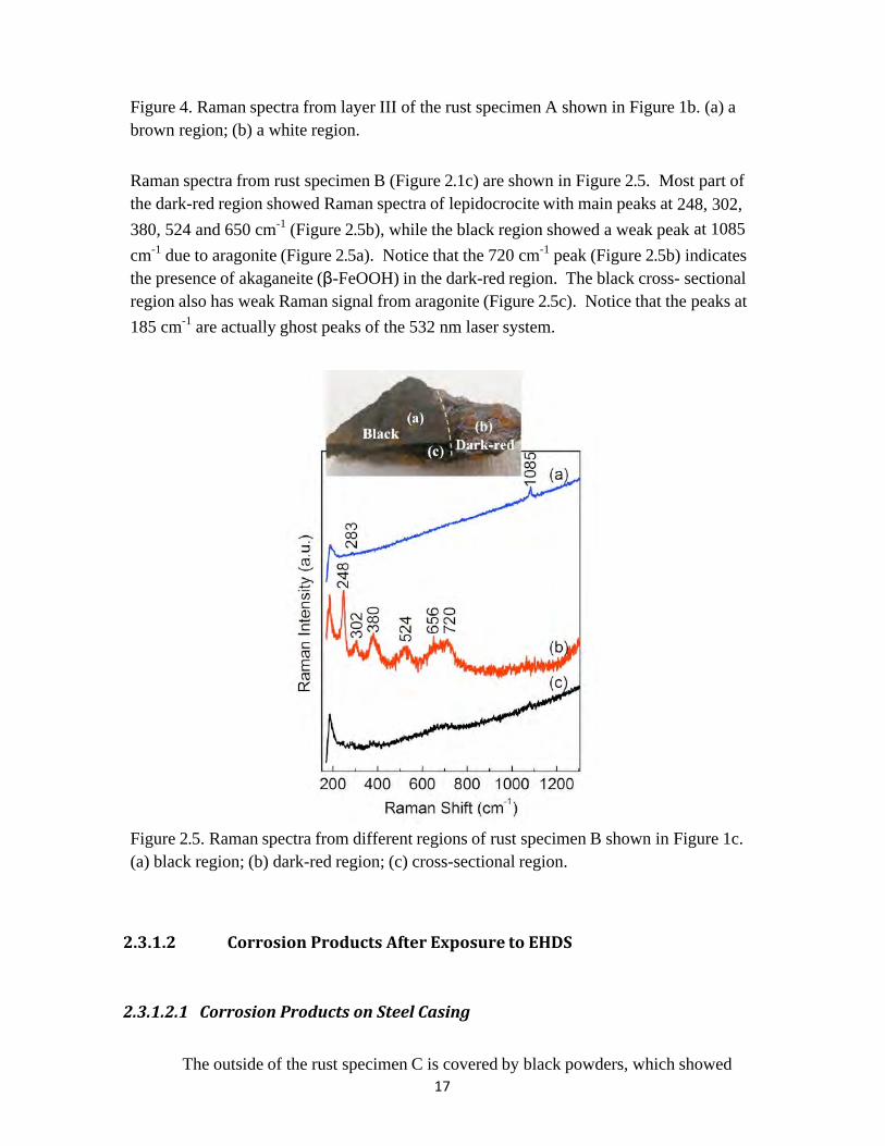
Figure 4. Raman spectra from layer III of the rust specimen A shown in Figure 1b. (a) a brown region; (b) a white region. Raman spectra from rust specimen B (Figure 2.1c) are shown in Figure 2.5. Most part of the dark-red region showed Raman spectra of lepidocrocite with main peaks at 248, 302, 380, 524 and 650 cm-1 (Figure 2.5b), while the black region showed a weak peak at 1085 cm-1 due to aragonite (Figure 2.5a). Notice that the 720 cm-1 peak (Figure 2.5b) indicates the presence of akaganeite (β-FeOOH) in the dark-red region. The black cross- sectional region also has weak Raman signal from aragonite (Figure 2.5c). Notice that the peaks at 185 cm-1 are actually ghost peaks of the 532 nm laser system.
Figure 2.5. Raman spectra from different regions of rust specimen B shown in Figure 1c. (a) black region; (b) dark-red region; (c) cross-sectional region.
2.3.1.2 Corrosion Products After Exposure to EHDS
2.3.1.2.1 Corrosion Products on Steel Casing
The outside of the rust specimen C is covered by black powders, which showed

18
Ram
an In
tens
ity (
a.u.
)
28
3 7
15
10
8
13
80
15
86
Raman spectra of carbon with two major peaks at 1354 and 1580 cm-1 (Figure 2.6b). Underneath the black powder, a gray layer (Figure 2.6a) showed weak Raman signal of akaganeite at 300 and 720 cm-1, and that of carbon at 1354 and 1580 cm-1. The black powder on the inside of rust specimen C showed strong peaks of carbon but also weak peaks at 291 and 411 cm-1, which are assigned to hematite (α-Fe2O3) (Figure 2.6c) [2]. The relatively strong peak at 666 cm-1 indicates the presence of a considerable amount of magnetite (Figure 2.6c) [2]. A region with red powders showed prominent peaks of hematite at 221, 291, 411, 495, 606, 656 and 1315 cm-1 (Figure 2.6d) [2]. The yellow rust in this rust specimen also has Raman signal of hematite (Figure 2.6e).
(a)
(b)
(c)
0 400 800 1200 1600 Raman Shift (cm-1)
(a) (b) Figure 2.6. a) Raman spectra from different locations of the rust specimen C shown in Figure 2.1d: Spectrum a - gray layer underneath the black powder on the outside; spectrum b - black powder on the outside; spectrum c - black powder in the inside; spectrum d - red rust; spectrum e - yellow rust. b) Raman spectra from different locations of the calcareous deposits on the copper rotating band shown in Figure 2.1e. Spectrum a – top surface of white layer; spectra b and c – black underside of white layer.
2.3.1.2.2 Products on Copper Rotating band
The top surface of the white layer bonded on top of the copper rotating band showed a Raman signal of siderite (FeCO3) with major peaks at 283, 715, and 1088 cm-1

19
(spectrum a, Figure 2.6b). The black deposit on the underside (region in contact with the copper rotating band) showed Raman signal of siderite in some regions together with weak Raman signal of carbon (i.e., peaks at 1380 and 1586 cm-1) (spectrum c, Figure 2.6b). Some regions of the black deposit showed Raman signal of pure carbon (spectrum b, Figure 2.6b). The carbon may have come from organic compounds pyrolyzed during processing in the EHDS.
2.3.2 SEM/EDXA results
2.3.2.1 Corrosion Products from Steel Casing Before Exposure to EHDS
SEM images and EDXA results from the four layers of the rust specimen A are shown in Figures 2.7 and 2.8, respectively. The first layer has a cotton-ball microstructure typical of steel rust (Figure 2.7a).
Figure 2.7. SEM images of the four layers of the rust specimen A. (a) layer I; (b) layer II; (c) layer III; (d) layer IV.
The high contents of Fe and O in this layer also suggest iron oxide as the major component (Figure 2.8a). Figure 2.7b and c show the fracture morphologies of layers II and III, respectively. The crystal facets of certain minerals can be seen in the two SEM images. EDXA results indicate that the minerals in layer II are mainly FeCO3 and CaCO3
(Figure 2.8b), while that in layer III is mostly CaCO3

20
(Figure 2.8c). Since Raman spectroscopic characterization showed that aragonite was the major component of layer III (Figure 2.4), it is reasonable to expect that the CaCO3 in layers II and III is aragonite rather than calcite. Therefore, the possibility of the two Raman peaks at 281 and 1083 cm-1 in Figure 2.3 coming from calcite can be eliminated. The fourth layer showed a porous, needle-like morphology (Figure 2.7d). A very high content of Ca suggests CaCO3 as the major component, which was proved to be aragonite by Raman spectroscopy (Figure 2.2d).
Figure 2.8. EDXA results from the four layers of the rust specimen A. (a) layer I; (b) layer II; (c) layer III; (d) layer IV. The regions from where EDXA results were obtained are approximately 20 µm × 20 µm in the center of the SEM images shown in Figure 2.7.
Figures 2.9 and 2.10 show the SEM images and EDXA results from the rust specimen B, respectively. The morphology of the black region (Figure 2.9a and b) is similar to that shown in Figure 2.7b, typical of the fracture surface of the inside of the rust pieces. EDXA results from this region indicate a relatively high content of Cu in some regions (Figure 2.10a), which is due to the fact that these regions could have been in contact with the copper rotating bands. The dark-red region (Figure 2.9c) has a
21
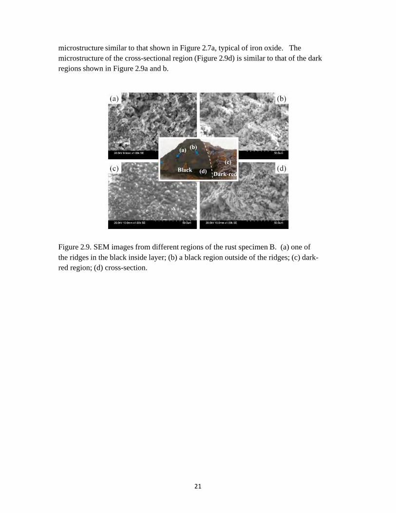
microstructure similar to that shown in Figure 2.7a, typical of iron oxide. The microstructure of the cross-sectional region (Figure 2.9d) is similar to that of the dark regions shown in Figure 2.9a and b.
Figure 2.9. SEM images from different regions of the rust specimen B. (a) one of the ridges in the black inside layer; (b) a black region outside of the ridges; (c) dark-red region; (d) cross-section.

22
Figure 2.10. EDXA results from different regions of the rust specimen B. (a) one of the ridges in the black inside layer; (b) a black region outside of the ridges; (c) dark-red region; (d) cross-section. The regions from where EDXA results were obtained were approximately 20 µm × 20 µm in the center of the SEM images shown in Figure 2.9.

23
2.3.2.2 Corrosion Products After Exposure to EHDS
Figures 2.11 and 2.12 show the SEM images and EDXA results from rust specimen C, respectively. The black powders from the outside had a very high content of C (Figure 2.12b), which came from the pyrolyzed organic materials that were attached to the DMM. The relatively high concentrations of potassium (K) and chlorine (Cl) (Figure 2.2b) are believed to come from sea salts originally. However, the reason why K is only present in the black powder on the outside of the rust specimen C, while other sea salt constituents (i.e., Na, Mg) were not detected is not clear.
Figure 2.11. SEM images from different regions of the rust specimen C. (a) a gray layer underneath the outer black powder; (b) outer black powder; (c) black powder in the inside; (d) red powder; (e) yellow powder. Other typical regions of this specimen (a: gray, c: red, d: black and e: yellow) have similar composition with high contents of Fe and O (Figure 2.12a, c, d and e), even though the observed morphologies are different (Figure 2.11a, c, d and e). The gray region is relatively compact while the others are porous. Notice that the rust crystals in the red region possess a well-defined pillar structure (Figure 2.11d). Also notice that
24
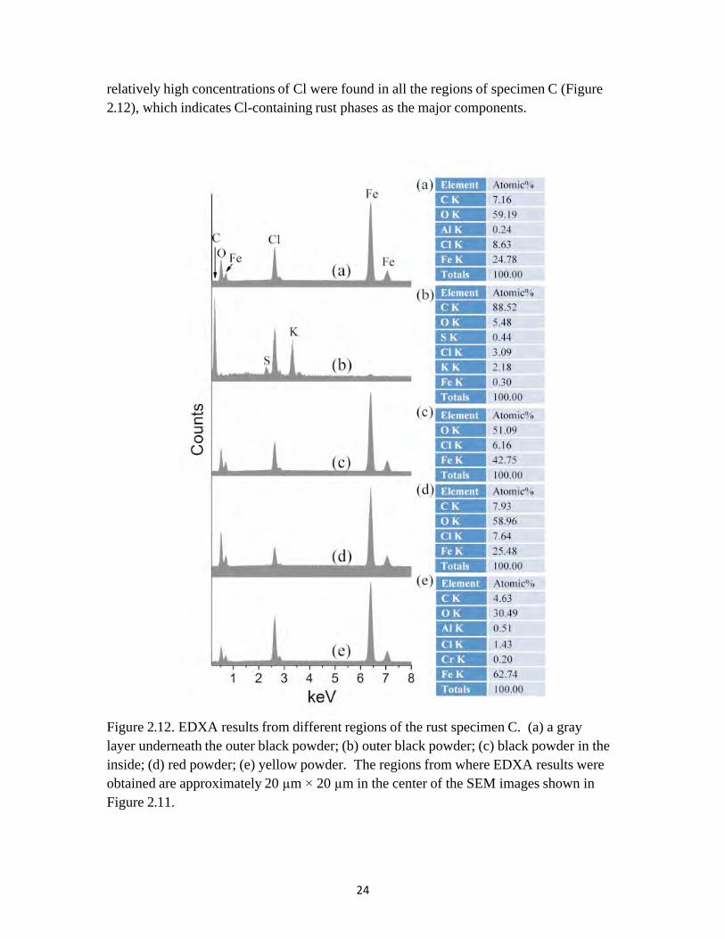
relatively high concentrations of Cl were found in all the regions of specimen C (Figure 2.12), which indicates Cl-containing rust phases as the major components.
Figure 2.12. EDXA results from different regions of the rust specimen C. (a) a gray layer underneath the outer black powder; (b) outer black powder; (c) black powder in the inside; (d) red powder; (e) yellow powder. The regions from where EDXA results were obtained are approximately 20 µm × 20 µm in the center of the SEM images shown in Figure 2.11.

25
2.3.3 XRD results
2.3.3.1 Corrosion Products from Steel Casing Before Exposure to EHDS
The XRD pattern (Figure 2.13a) from powders made of layers II and III of rust specimen A shows intense peaks of siderite, magnetite and aragonite [1], indicating they are the major components in the inner layers.
Figure 2.13. Powder XRD patterns of the rust pieces A and B. (a) powder made from the rust marked by region 1 in Figure 2.1b, representing layers I and II of the rust specimen A; (b) powder made from the coral layer marked by region 2 in Figure 2.1b, representing layer IV of the rust specimen A; (c) powder made from the rust flakes scratched from the black region shown in Figure 2.1c.

26
A small amount of akaganeite and lepidocrocite were also detected with extremely weak peaks (Figure 2.13a). Not surprisingly, powders made from the yellow coral layer showed XRD pattern of pure aragonite (Figure 2.13b). Powders made from the inner layer of the rust specimen B showed an XRD pattern (Figure 2.13c) similar to that shown in Figure 2.13a, but with weaker peaks from aragonite. This result indicates that siderite and aragonite are the major components in the inner layers of the rust specimens.
2.3.3.2 Corrosion Products After Exposure to EHDS
More corrosion product phases were detected from the rust specimen C (Figure 2.14). The XRD pattern of the black powder from the outside of the rust specimen C showed the presence of a considerable amount of magnetite and hematite (Figure 2.14a). Weak XRD peaks originated from α–Fe2(OH)3Cl and akaganeite suggest a small amount of those species in the black powder. Notice that an XRD peak for carbon was also detected, which agrees with the Raman spectroscopic characterization results shown in Figure 2.6 and the EDXA result shown in Figure 2.12b. The carbon is likely the result of the pyrolysis process used in the EHDS. Also notice that the detected XRD peaks for KCl corroborate the EDXA results shown in Figure 2.12b. The XRD pattern of black powder in the inside the rust specimen C showed α–Fe2(OH)3Cl, magnetite and akaganeite as the major components (Figure 2.14b). XRD patterns from other regions of this rust specimen were similar to that shown in Figure 2.14b, but with weaker peaks for magnetite and akaganeite (Figure 2.14c and d). The peaks at 22.40 and 29.71 degrees (question marks) are not yet identified.

27
Figure 2.14. Powder XRD patterns of the rust specimen C. (a) powder from the outer surface of the rust specimen C; (b) powder from the inside layer of the rust specimen C; (c) powder made from the rust specimen marked by the solid rectangular region 1 in Figure 1d; (d) powder made from the rust marked by the solid rectangular region 2 in Figure 2.1d.
28
2.4 Discussion As a micro-analysis technique, Raman spectroscopy is able to distinguish various corrosion product phases at the micron scale. During the Raman spectroscopic characterization of the rust from the DMM, lepidocrocite was detected in certain regions (Figures 2.2a and 2.5b). However, XRD results show only a very weak peak for lepidocrocite (Figure 2.13a). Therefore, XRD is superior to Raman spectroscopy in determining the relative amounts of the various rust phases. Another discrepancy between the XRD and Raman results is the detection of mackinawite. Since mackinawite is not stable [5], it may only exist in wet conditions (for Raman analysis) and transformed into other phases after the dehydration of the sample in a dry box (for XRD analysis). Another reason why mackinawite was not detected using XRD might be due to the relatively small amount of S as indicated by the EDXA results (Figures 2.8, 2.10 and 2.12). A third discrepancy between the XRD and Raman results is the detection of gypsum. It is possible that only a small amount of gypsum presents in the inner layers of rust specimen A and did not generate prominent XRD peaks.
Although offering only elemental information, EDXA results helped distinguish various compounds that did not show any difference during Raman analysis. For example, the EDXA results in Figure 2.8 indicate the presence of siderite instead of calcite in the layer II of the rust specimen A. Also, EDXA results corroborate the XRD analysis. The high content of Cl (Figure 2.12) in the pyrolyzed rust layer agrees well with the detection of α–Fe2(OH)3Cl using XRD analysis (Figure 2.6). Another interesting EDXA result was the elemental distributions of Fe, Cl and Ca over the cross-section of the rust pieces, as summarized in Figure 2.15. Since iron oxide formed in the inner layers of the rust-and-coral layer and coral are in the outer layers, higher content of Fe occurred in the inner layers and higher content of Ca occurred in the outer layers (Figure 2.15). The reason why Cl has a higher content in the inner layers is due to the migration of Cl ions from seawater to the actively dissolving metal/corrosion product interface. The hydrolysis of Fe2+ generated by corrosion rendered an acidic environment with excess positive charge, which attracts Cl- anions by migration from the surrounding solution.

29
Figure 2.15. Concentration profiles (atomic % from EDXA) of Fe, Cl and Ca across the cross-section of the rust pieces.
Raman spectroscopy, which enabled phase identification on the micron scale, is complementary to powder XRD analysis, which showed detailed phase information of a bulk corrosion product. The pyrolyzed rust layer (specimen C) is composed of mainly α–Fe2(OH)3Cl, with formation facilitated by high content of Cl (Figure 2.12), and likely the high temperature in the EHDS. Since α–Fe2(OH)3Cl was absent from specimens A and B, which were removed from the DMM before the EHDS process, it is likely that elevated temperature induced the formation of α–Fe2(OH)3Cl.
For specimens A and B, which were not subjected to pyrolysis, the Fe-containing species found in the layer near to the DMM surface were lepidocrocite (γ-FeOOH), magnetite (Fe3O4), akaganeite (β-FeOOH), and mackinawite (FeS). Previous work [5] has found β–Fe2(OH)3Cl as the main phase precipitated on an iron ingot immersed in the sea for 2000 years. This iron hydroxychloride was believed to be characteristic of corrosion in anoxic and chlorinated medium. A possible reason for the discrepancy between our results and those from literature is that γ-FeOOH and (β-FeOOH) form in relatively short-time immersion (60+ years in this study) and ages to β–Fe2(OH)3Cl after very long immersion times (up to 2000 years). The presence of magnetite was related to a process before marine corrosion[5]. It is believed that the hot forging process of the ingot might have generated a magnetite layer. However, the exact source of magnetite formed on the projectile is not clear. The presence of FeS is likely related to the presence of sulfate reducing bacteria.
The intermediate rust layer is mainly composed of siderite. The formation of siderite is associated with intense bacterial activity and the concomitant large amount of carbon dioxide and carbonate species[5].

30
2.5 Conclusion
Using three complementary techniques, the rust species that formed on DMMs immersed in the ocean for 60+ years were successfully identified. The main phases in the innermost rust layer are lepidocrocite (γ-FeOOH) and magnetite (Fe3O4). Siderite (FeCO3) was detected as the major component of the intermediate rust layer in between the innermost rust layer and the outer coral layer.
2.6 References 1. ICDD, International Centre for Diffraction Data PDF-2 2008. 2. deFaria, D.L.A., S.V. Silva, and M.T. deOliveira, Raman microspectroscopy of
some iron oxides and oxyhydroxides. Journal of Raman Spectroscopy, 1997. 28: p. 873-878.
3. RRUFF™, Gypsum. http://rruff.info/chem=s,%20o/display=default/R040029. 4. Ph. Refait, D.D.N., M. Jeannin, S. Sable, M. Langumier, R. Sabot,
Electrochemical formation of green rusts in deaerated seawater-like solutions. Electrochimica Acta, 2011. 56: p. 6481-6488.
5. Rémazeilles, C., et al., Mechanisms of long-term anaerobic corrosion of iron archaeological artifacts in seawater. Corrosion Science, 2009. 51: p. 2932-2941. 6. Pineau, S., et al., Formation of the Fe(II–III) hydroxysulphate green rust during
marine corrosion of steel associated to molecular detection of dissimilatory sulphite-reductase. Corrosion Science, 2008. 50: p. 1099-1111.
7. Boughriet, A., et al., Identification of newly generated iron phases in recent anoxic sediments: 57Fe Mossbauer and micro-Raman spectroscopic studies. Journal of Chemical Society Faraday Transactions, 1997. 93: p. 3209-3215.
8. Bourdoiseau, J.A., et al., Characterisation of mackinawite by Raman spectroscopy: Effects of crystallisation, drying and oxidation. Corrosion Science, 2008. 50: p. 3247-3255.
9. RRUFF™, Aragonite. http://rruff.info/chem=ca,%20c,%20o/display=default/R040078. 10. RRUFF™, Siderite. http://rruff.info/siderite/display=default/R040034. 11. RRUFF™, Calcite. http://rruff.info/calcite/display=default/R040070. 12. WU, http://eps.wustl.edu/files/epsc/BUF_Figure1_5.pdf, (Washington Univeristy
in St. Louis, Department of Earth and Planetary Sciences).

31
3 Part 2: Corrosion Experimentation with DMM Steel Casing and Copper Rotating Band Materials
3.1 Objective
The objectives of this research were 1) to conduct metallographic analysis on the munitions to identify the alloying elements in the steel casing and copper rotating bands, and 2) to understand the galvanic corrosion between the steel casings and the copper rotating bands. Potentiodynamic polarization and zero-resistant ammeter (ZRA) electrochemical experiments were conducted on electrodes made from the steel casing and copper rotating band in simulated (sodium chloride and ASTM seawater solutions) and real seawater. Polarization experiments were used to identify the governing corrosion mechanisms, and ZRA experiments were used to determine the steady-state galvanic current density (iGalv (A/cm2)) between steel and copper. The steady-state values in ZRA experiments were the average values for the last 20 hours of the experiments. Results from polarization and ZRA experiments conducted in the simulated seawaters were correlated. The iGalv from long-term ZRA experiments were used to calculate the corrosion rate in grams per meter squared per day (gmd) using Faraday’s law. Electrodes from polarization and ZRA experiments were analyzed with a Hitachi S- 3400N Scanning Electron Microscopy (SEM) and Oxford Instruments Energy Dispersive
X-ray Analysis (EDXA) for elemental analysis.
3.2 Background
Steel munitions casings coupled to copper is susceptible to galvanic corrosion. Galvanic corrosion is defined as accelerated corrosion of a metal due to electrical contact with a more noble metal in a corrosive environment [1]. The material, which usually has a lower corrosion potential (ECorr) or open circuit potential (OCP), is more active and acts as the anode where oxidation takes place. The material, which has a higher (positive) ECorr, is less active or more noble and acts as the cathode where hydrogen evolution and/or oxygen reduction take place.
The three conditions for a galvanic couple to exist are:
1. At least two different conductive materials must be involved 2. The materials must be in electrical contact so that current can flow between them

32
3. Both materials must be submersed in a corrosive medium or electrolyte
If any one of these three conditions is removed, galvanic corrosion will not occur [2].
Steel alloys generally become anodic when coupled to copper because they are more active than copper in the galvanic series [3]. At the anode, Fe2+ ions and electrons are generated (equation 1) as a result of oxidation in the galvanic cell. These electrons are consumed at the copper cathode surface (more noble metal) either by hydrogen evolution (equation 2), oxygen reduction (equation 3), or both. Hydrogen evolution takes place if the cell is deaerated. The H+ protons are formed as a result of water dissociation (H2O = H+ + OH-). Oxygen reduction and/or hydrogen evolution take place if the cell is aerated.
Anodic reaction:
(1) Cathodic reactions:
1. Hydrogen evolution: (2)
2. Oxygen reduction: (3)
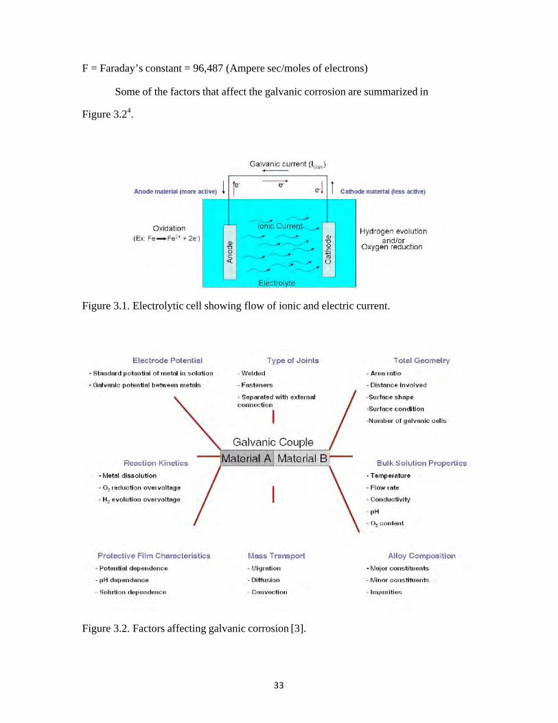
The flow of electrons causes a current flow in the electric conductor equal in
magnitude to the ionic current flowing in the opposite direction in the electrolyte (Figure 3.1). Lack of electrolyte or an electrolyte void of charge carriers ceases the ionic current, thus limiting galvanic corrosion.
According to Faraday’s law (equation 4), the amount of current flowing between the anode and the cathode is directly proportional to the amount of anodic material (steel in this case) that is dissolved [4].
(4)
M = mass of Al dissolved to produce galvanic current (g) Ar = atomic weight of Fe (g) ICorr = current generated (Amperes)
t = time (sec)
n = moles of electrons per moles of Fe reacted
33
F = Faraday’s constant = 96,487 (Ampere sec/moles of electrons)
Some of the factors that affect the galvanic corrosion are summarized in
Figure 3.24.
Figure 3.1. Electrolytic cell showing flow of ionic and electric current.
Figure 3.2. Factors affecting galvanic corrosion [3].

34
3.3 Experimental Procedure
3.3.1 Material Characterization Steel and copper samples were sand blasted and cut from the demilitarized DMM.
The samples were then ground using a Buehler Ecomet® 6 variable speed grinder- polisher and with 180-grit SiC paper followed by 320-grit and 600-grit SiC papers. Samples were then successively polished to a mirror-like finish using Buehler micro- cloth and slurries of 1 micron alpha alumina, 0.3 micron alpha alumina, and 0.05 micron gamma alumina powder. The samples were then examined with SEM and EDXA for elemental analysis.
Polished steel and copper samples were also chemically analyzed by Hurst Metallurgical Research Laboratory, Inc., Texas. Chemical analysis test was performed using Thermo Jarell Ash AtomComp 81, S/N 26094 optical emission spectrometer with Angstron S-1000 readout and control systems [5].
3.3.2 Polarization Experiments
Anodic polarization of steel and cathodic polarization of copper electrode was conducted with a Princeton Applied Research PARSTAT 2273 potentiostat. Steel and copper electrodes were prepared with an exposed surface area of 1 cm2. The electrical connections were made using a copper wire and silver conductive epoxy (MG Chemicals 8331-14g) and cured in an oven at 70oC for 20 minutes. The metal samples were then mounted in a 0151 Hysol epoxi-patch adhesive and glass tubes and cured in an oven at 70oC for 2 hours. The electrodes were ground using a Buehler Ecomet® 6 variable speed grinder-polisher. The surface area that was exposed was ground flat with 180-grit SiC paper followed by 320-grit, and 600-grit SiC papers. Electrodes were then successively polished to a mirror-like finish using Buehler micro-cloth and slurries of 1 micron alpha alumina, 0.3 micron alpha alumina, and 0.05 micron gamma alumina powder. Figure 3.3 shows a typical steel and copper electrode.
35
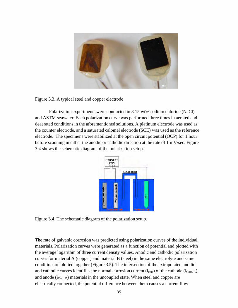
Figure 3.3. A typical steel and copper electrode
Polarization experiments were conducted in 3.15 wt% sodium chloride (NaCl) and ASTM seawater. Each polarization curve was performed three times in aerated and deaerated conditions in the aforementioned solutions. A platinum electrode was used as the counter electrode, and a saturated calomel electrode (SCE) was used as the reference electrode. The specimens were stabilized at the open circuit potential (OCP) for 1 hour before scanning in either the anodic or cathodic direction at the rate of 1 mV/sec. Figure 3.4 shows the schematic diagram of the polarization setup.
Figure 3.4. The schematic diagram of the polarization setup.
The rate of galvanic corrosion was predicted using polarization curves of the individual materials. Polarization curves were generated as a function of potential and plotted with the average logarithm of three current density values. Anodic and cathodic polarization curves for material A (copper) and material B (steel) in the same electrolyte and same condition are plotted together (Figure 3.5). The intersection of the extrapolated anodic and cathodic curves identifies the normal corrosion current (icorr) of the cathode (iCorr, A) and anode (iCorr, B) materials in the uncoupled state. When steel and copper are electrically connected, the potential difference between them causes a current flow

36
between them, which could be measured using an ammeter. This measured current is equal to the galvanic current (iGalv) that is identified at the intersection of the cathodic curve of material A (the cathode) and the anodic curve of material B (the anode). The galvanic current between the electrodes is higher than the normal corrosion current iCorr,B
of material B, which is the anode in the galvanic couple. This increase in current due to galvanic effect causes corrosion rate of the active material B (steel) to increase when electrically coupled to a noble material A (copper) in a corrosive environment. It should also be noted that the galvanic current does not account for local corrosion on the anode that is caused by cathodic reactions simultaneously occurring on the anode. Depending on the materials in the galvanic couple and the environment, the local corrosion on the anode may or may not be negligible. The total corrosion of the anode in the galvanic couple is equal to the galvanic component plus the local component.
Figure 3.5. Hypothetical polarization curves
3.3.3 Artificial Seawater ZRA Experiment
The change in galvanic corrosion rate over a period of time was measured using
the ZRA technique. Short-circuit current between the two electrically connected materials is related to the rate of the mass loss of the active metal due to the galvanic effect [6].
The steel and cooper electrodes were fabricated with a surface area of 2 cm2
(Figure 3.6). Electrodes were prepared similar to the procedure explained in the polarization experiment section (see section 4.2).

37
Figure 3.6. Steel-copper electrode couple for short-term ZRA experiments
The ZRA experiments were conducted in a three-electrode setup in 3.15 wt% NaCl, and ASTM seawater. A saturated calomel electrode (SCE) was used as a reference electrode to measure the galvanic potential (EGalv). Ionic contact between the electrolytic cell and the reference cell was made by a Luggin (capillary) probe. The iGalv and the EGalv
values of the couple were measured using a ZRA manufactured by ACM Instruments. Measured iGalv and EGalv values were recorded in VOLT101 data loggers manufactured by MadgeTech, Inc., NH. Figure 3.7 shows the schematic diagram of the ZRA connections. Resistance through the electrolyte was minimized by placing the steel and copper electrodes side by side with the exposed electrode areas immersed in the solution. The tip of the Luggin probe was placed within a few millimeters to the exposed area of the electrode. The iGalv and corresponding EGalv for each experiment were recorded with data loggers every 15 seconds for 5 days to achieve steady state values.
Figure 3.7. The schematic diagram of the ZRA setup.
3.3.4 Cell Conditions
The electrolytic cell for polarization and short-term ZRA experiments was a
jacketed vessel in which the temperature was maintained at 30oC using a Fisher Scientific

38
Isotemp refrigerated circulator 9500. The cell was aerated by sparging compressed air through a fritted glass dispersion tube at volumetric rate of 320-370 ml/minute at 1 atmospheric pressure. The natural convection in the cell was kept relatively constant for each experiment by maintaining a uniform gas dispersion rate. The deaerated condition was achieved by sparging the cell with nitrogen gas with a purity of at least 99.999%. 3.3.5 Real Seawater ZRA Experiments The iGalv between steel and copper electrodes were measured in real seawater for 14 days. The electrical connection between steel and copper electrodes immersed in real seawater was made through a 330-ohm resistor and MadgeTech Volt 101A-160mv data logger to measure iGalv. The SCE was placed inside the same cell where the electrodes were placed and was connected electrically to the steel electrode through a MadgeTech Volt 101A data logger to measure EGalv. The iGalv and corresponding EGalv for each couple were recorded with data loggers every 15 seconds for 14 days to achieve steady state values.
Three sets of steel-copper couples were placed in a two-liter cell (i.e., a bucket). Another three sets of steel-copper couples were placed in another two-liter cell buried in sea sand to a depth of 2 inches (Figure 3.8). The two cells were fixed to the bottom of 30 in. x 12.5 in. x 12.5 in. glass tank (aquarium) using silicone sealant. Real seawater was then added to the tank (approximately five gallons) so that the two cells were completely immersed inside the seawater. The glass tank was maintained at 30oC using an automatic aquarium heater. One aquarium pump was installed inside each glass tank to circulate the water in the bath. This setup maintained a uniform temperature and natural convection throughout the glass tank. The glass tank was partially covered to keep the evaporation of the solution to a minimum. The partial covering of the glass tank also ensured an aerated condition. The dissolved oxygen inside the two cells was measured using a HOBO Dissolved Oxygen logger. Figure 3.8 shows the schematic setup with couples immersed in different conditions inside the glass tank. Figure 3.9 shows a photo of the actual apparatus.
Figure 3.8. The schematic diagram of the long-term ZRA setup.
39
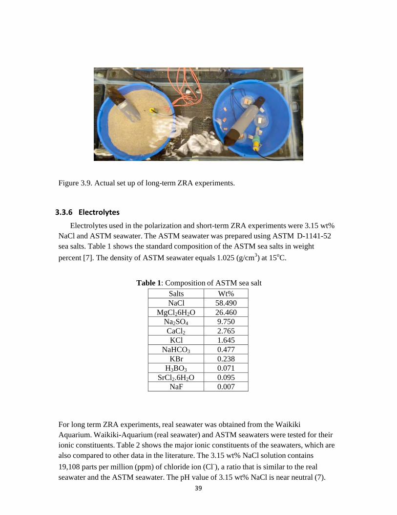
Figure 3.9. Actual set up of long-term ZRA experiments.
3.3.6 Electrolytes Electrolytes used in the polarization and short-term ZRA experiments were 3.15 wt%
NaCl and ASTM seawater. The ASTM seawater was prepared using ASTM D-1141-52 sea salts. Table 1 shows the standard composition of the ASTM sea salts in weight percent [7]. The density of ASTM seawater equals 1.025 (g/cm3) at 15oC.
Table 1: Composition of ASTM sea salt
Salts Wt% NaCl 58.490
MgCl26H2O 26.460 Na2SO4 9.750 CaCl2 2.765 KCl 1.645
NaHCO3 0.477 KBr 0.238
H3BO3 0.071 SrCl2.6H2O 0.095
NaF 0.007
For long term ZRA experiments, real seawater was obtained from the Waikiki Aquarium. Waikiki-Aquarium (real seawater) and ASTM seawaters were tested for their ionic constituents. Table 2 shows the major ionic constituents of the seawaters, which are also compared to other data in the literature. The 3.15 wt% NaCl solution contains 19,108 parts per million (ppm) of chloride ion (Cl-), a ratio that is similar to the real seawater and the ASTM seawater. The pH value of 3.15 wt% NaCl is near neutral (7).

40
The pH values of ASTM seawater and real seawater were 8.2 and 7.9, respectively.
Table 2: The major ionic constituents of different types of seawater
Ions
Waikiki* (ppm)
ASTM
Seawater* (ppm)
IAPSO (ppm)
The Oceans, Prentice- Hall,Inc.,
New York,1942 (ppm) Calcium, Ca++
429.50 516.66 432 400.1
Magnesium, Mg++
1513.58
1731.60
1348
1272
Sodium, Na+ 10461.5 10118 11266 10556.1
Potassium, K+ 356.13 396.74 411 380
Chloride, Cl- 19581.5 20488 19900 18980
Sulfate, SO4--
2663.46 2596.6 2712 2649 Bromide, Br-
61.10 141.57 67 64.6 *Analysis performed by Dr. Huebert, Dept. of Oceanography, University of Hawai‘i.
Sea sand in shoreline water was collected off the coast of Waianae, close to Ordnance Reef (HI-06) (Figure 3.10). The geographic coordinates of the sea sand collection location are listed in Table 3.
Table 3: geographic coordinates of the sea sand pick up location
Latitude Longitude
N 21.537187 W 158.231694
Figure 3.10. Oahu map.

41
3.4 Results and Discussion
3.4.1 Material Characterization
Figure 3.11 shows steel casing and copper rotating band of a DMM similar to that used in this study. Preliminary elemental analyses were conducted in-house using EDXA.
(a) (b)
Figure 3.11. a) steel casing of DMM, and b) copper rotating band on steel casing of DMM.
Figure 3.12 shows the SEM image and EDXA results of steel samples. The weight and atomic percentage of the steel samples obtained from EDXA are shown in Table 4. The major elemental composition of the DMM steel samples consists of iron, carbon, manganese, and aluminum. The origin of aluminum is likely due to residue from polishing with alumina powder, and the carbon may be due a combination of carbon present in the steel, hydrocarbon contamination, or pyrolysis of organic materials during energetic hazard demilitarization system (EHDS) treatment of DMM at HI-06 prior to sample receipt.
Figure 3.13 shows the SEM image and EDXA results of copper samples. The weight and atomic percentage of the copper samples obtained from EDXA are shown in Table 5. The major elemental composition of copper samples consists of copper, carbon, aluminum, and silicon. The origin of aluminum and silicon is likely due to residue from polishing with alumina powder and grinding with silicon carbide grinding paper, respectively, and the carbon may be due to hydrocarbon contamination or pyrolysis of organic materials during EHDS treatment.

42
a b
Figure 3.12. SEM (a) and EDXA (b) results of steel samples
Table 4: The weight and atomic percentage of the steel samples Element Weight% Atomic%
C K 4.75 18.48 Al K 0.77 1.33 Mn K 0.81 0.69 Fe K 95.05 79.50
(a) (b)
Figure 3.13. SEM (a) and EDXA (b) results of copper samples
Table 5: The weight and atomic percentage of the copper samples
Element
Weight%
Atomic% C K 17.94 47.04 O K 4.71 9.27 Al K 0.49 0.57 Si K 2.31 2.60 Cu L 81.74 40.53
43
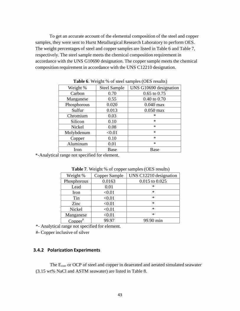
To get an accurate account of the elemental composition of the steel and copper samples, they were sent to Hurst Metallurgical Research Laboratory to perform OES. The weight percentages of steel and copper samples are listed in Table 6 and Table 7, respectively. The steel sample meets the chemical composition requirement in accordance with the UNS G10690 designation. The copper sample meets the chemical composition requirement in accordance with the UNS C12210 designation.
Table 6. Weight % of steel samples (OES results) Weight % Steel Sample UNS G10690 designation
Carbon 0.70 0.65 to 0.75 Manganese 0.55 0.40 to 0.70
Phosphorous 0.020 0.040 max Sulfur 0.013 0.050 max
Chromium 0.03 * Silicon 0.10 * Nickel 0.08 *
Molybdenum <0.01 * Copper 0.10 *
Aluminum 0.01 * Iron Base Base
*-Analytical range not specified for element.
Table 7. Weight % of copper samples (OES results) Weight % Copper Sample UNS C12210 designation
Phosphorous 0.0163 0.015 to 0.025 Lead 0.01 * Iron <0.01 * Tin <0.01 * Zinc <0.01 *
Nickel <0.01 * Manganese <0.01 *
Copper# 99.97 99.90 min
*- Analytical range not specified for element. #- Copper inclusive of silver
3.4.2 Polarization Experiments
The Ecorr or OCP of steel and copper in deaerated and aerated simulated seawater
(3.15 wt% NaCl and ASTM seawater) are listed in Table 8.

44
Table 8. The Ecorr or OCP (VSCE) of steel and copper in simulated seawater 3.15 Wt% NaCl
(Deaerated) 3.15 Wt% NaCl
(Aerated) ASTM Seawater
(Deaerated) ASTM Seawater
(Aerated) Steel -0.762 -0.624 -0.771 -0.612
Copper -0.352 -0.249 -0.354 -0.257
In both the deaerated and aerated conditions, the copper electrodes were significantly more noble than the steel electrodes; hence, the steel will be the anode and the copper will be the cathode in the galvanic couple. Hence, the steel should corrode at a higher rate in the galvanic couple compared to the uncoupled state.
Anodic curves of steel were obtained by polarizing the steel electrodes from the OCP in the positive direction, and cathodic curves of copper were obtained by polarizing the copper electrodes from the OCP in the negative direction. Figure 3.14 show the anodic curve of steel and cathodic curve of copper in deaerated 3.15 wt% NaCl.
Figure 3.14. Cathodic and anodic polarization of copper and steel in deaerated 3.15 wt % NaCl at 30 oc. Scan rate=1mv/s

45
Figure 3.15. Cathodic and anodic polarization of copper and steel in aerated 3.15 wt % NaCl at 30 oc. Scan rate=1mv/s.
The iGalv value in the deaerated condition was lower than the iGalv value in the aerated condition. The cathodic curve of copper in deaerated condition (due to hydrogen evolution) and the cathodic curve of copper in aerated condition (due to oxygen reduction) controls the galvanic current for the steel-copper couple in 3.15 wt% NaCl solution as the steel anodic curve does not readily polarize. The steel-copper couple is primarily under cathodic control.
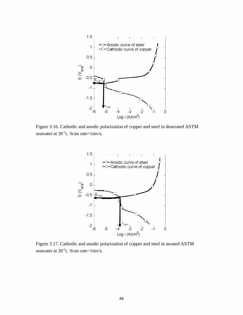
Figure 3.16 shows the anodic curve of steel and cathodic curve of copper in deaerated ASTM seawater. Figure 3.17 show the anodic curve of steel and cathodic curve of copper in aerated ASTM seawater. The iGalv value in the deaerated condition was lower than the iGalv value in the aerated condition. The iGalv and EGalv values in ASTM seawater were similar to that in 3.15 wt% NaCl (Table 9).
46
Figure 3.16. Cathodic and anodic polarization of copper and steel in deaerated ASTM seawater at 30 oc. Scan rate=1mv/s.
Figure 3.17. Cathodic and anodic polarization of copper and steel in aerated ASTM seawater at 30 oc. Scan rate=1mv/s.

47
Table 9. The iGalv (µA/cm2) and EGalv (VSCE) values in simulated seawater (polarization experiments) 3.15 Wt%
NaCl (Deaerated)
ASTM Seawater (Deaerated)
3.15 Wt% NaCl
(Aerated)
ASTM Seawater (Aerated)
iGalv (µA/cm2) 7.9 6.3 173 158 EGalv(VSCE) -0.749 -0.756 -0.569 -0.575
3.4.3 Artificial Seawater ZRA Experiments
Figure 3.18 shows the iGalv profile of steel coupled to copper in aerated 3.15 wt% NaCl and ASTM seawater obtained from ZRA experiments.
Figure 3.18. The iGalv profile of steel coupled to copper in aerated 3.15 wt% NaCl and ASTM seawater.
The steady state iGalv values of steel coupled to copper in aerated 3.15 wt% NaCl were significantly higher than the steady state iGalv values in aerated ASTM seawater. The difference in corrosion rates could be due to the presence of other ions in seawater, though Cl- concentrations of ASTM seawaters are comparable to the 3.15 wt% NaCl. Calcium and magnesium ions present in the seawater electrolytes can react with the hydroxyl ions (OH-) ions generated on the cathode as a result of oxygen reduction (and proton reduction) to form calcium carbonate and magnesium hydroxide films on the

48
copper surface (cathodic site) [8 and 9].
(precipitate) (5)
(precipitate) (6) This film formation lowered the galvanic corrosion rate in seawaters by stifling oxygen reduction at the cathodic sites. Dissolved carbon-di-oxide (CO2) in aqueous systems reacts to form carbonic acid (H2CO3) via the following reaction:
(7)
Carbonic acid dissociates into bicarbonate (HCO3-) and carbonate (CO3
2-) according to the following equations
(8)
(9)
The equilibrium constant Ka1 for the dissociation of carbonic acid into bicarbonate is 4.47 x 10⁻⁷ and the equilibrium constant Ka2 for the dissociation of bicarbonate into carbonate is 4.65 x 10⁻⁷. The pKa1 and pKa2 values are 6.35 and 10.35, respectively [10].
Figure 3.19 shows a graphical summary of the relative concentrations of the three carbonate species (H2CO3, HCO3
-, and CO32-) in the pH range of 0 to 14.
Figure 3.19. The distribution of carbonate species as a fraction of total dissolved carbonate (CT) in relation to solution pH [10].

49
As mentioned earlier, the pH values of ASTM seawater and real seawater were 8.2 and 7.9, respectively. At these pH values, the relative concentration HCO3
- is higher than the other carbonate species. The bicarbonate and hydroxyl ions (generated on the cathode) as a result of oxygen reduction in the aerated condition reacts with calcium ions present in the seawater to form calcium carbonate (equation 6).
Figure shows the SEM picture of copper electrode after short-term ZRA experiment in aerated ASTM seawater. EDXA results confirmed the deposits of calcium and magnesium (Figure 3.20 and Table 10).
Figure 3.20. SEM micrograph of copper electrode after short-term ZRA experiment in aerated ASTM seawater
Figure 3.21. EDXA results on copper electrode after short-term ZRA experiments in aerated ASTM seawater.
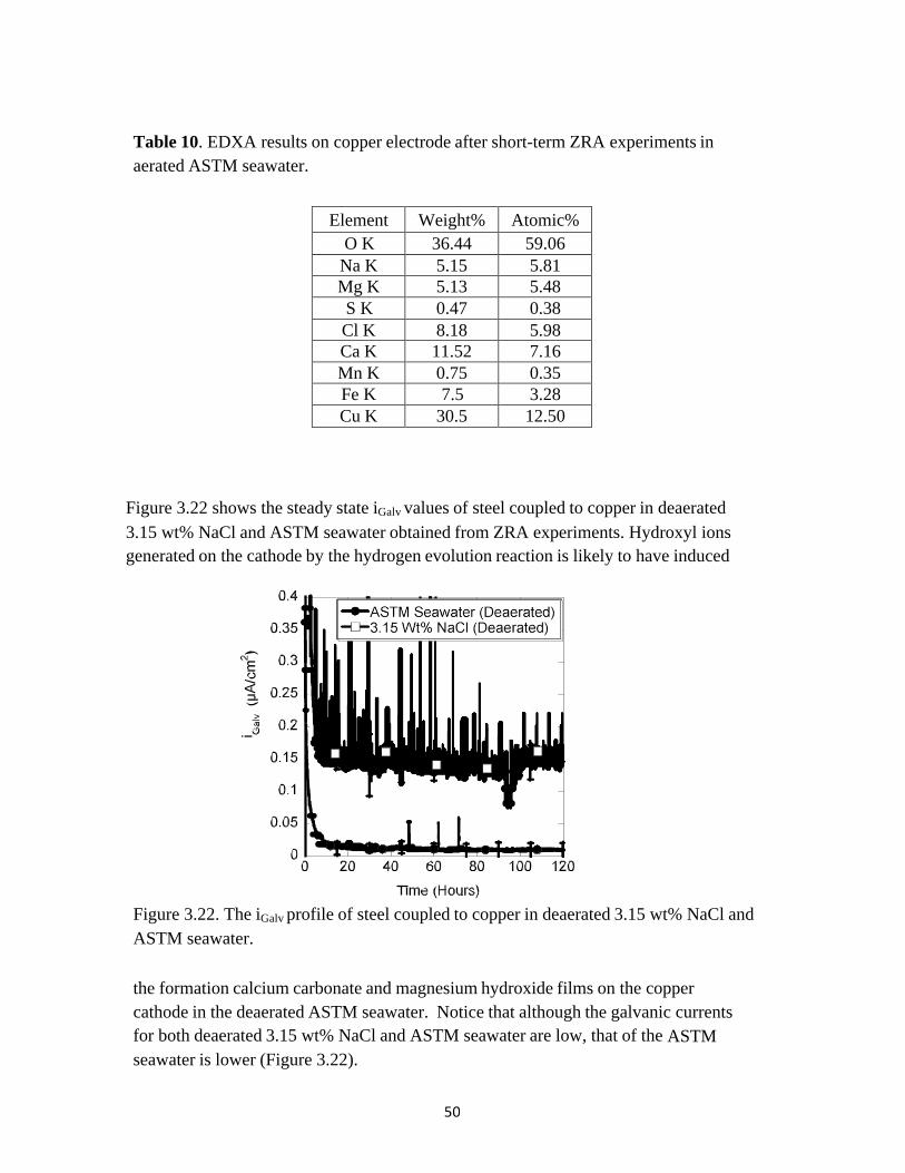
50
Table 10. EDXA results on copper electrode after short-term ZRA experiments in aerated ASTM seawater.
Element Weight% Atomic% O K 36.44 59.06
Na K 5.15 5.81 Mg K 5.13 5.48 S K 0.47 0.38 Cl K 8.18 5.98 Ca K 11.52 7.16 Mn K 0.75 0.35 Fe K 7.5 3.28 Cu K 30.5 12.50
Figure 3.22 shows the steady state iGalv values of steel coupled to copper in deaerated 3.15 wt% NaCl and ASTM seawater obtained from ZRA experiments. Hydroxyl ions generated on the cathode by the hydrogen evolution reaction is likely to have induced
Figure 3.22. The iGalv profile of steel coupled to copper in deaerated 3.15 wt% NaCl and ASTM seawater.
the formation calcium carbonate and magnesium hydroxide films on the copper cathode in the deaerated ASTM seawater. Notice that although the galvanic currents for both deaerated 3.15 wt% NaCl and ASTM seawater are low, that of the ASTM seawater is lower (Figure 3.22).
51
The polarization results in aerated seawaters were similar to those in 3.15 wt% NaCl; whereas, the galvanic corrosion rates in seawaters were lower than those in 3.15 wt% NaCl solution based on the steady-state values from ZRA experiments. The steady state iGalv values from the ZRA experiments were recorded after 120 hours; whereas, the polarization experiments were run for 1 to 2 hours to obtain the iGalv
value. The ZRA iGalv values at the initial period were comparable with the polarization iGalv values. This observation may indicate that a calcareous film have precipitated on cathodic copper electrodes over time.
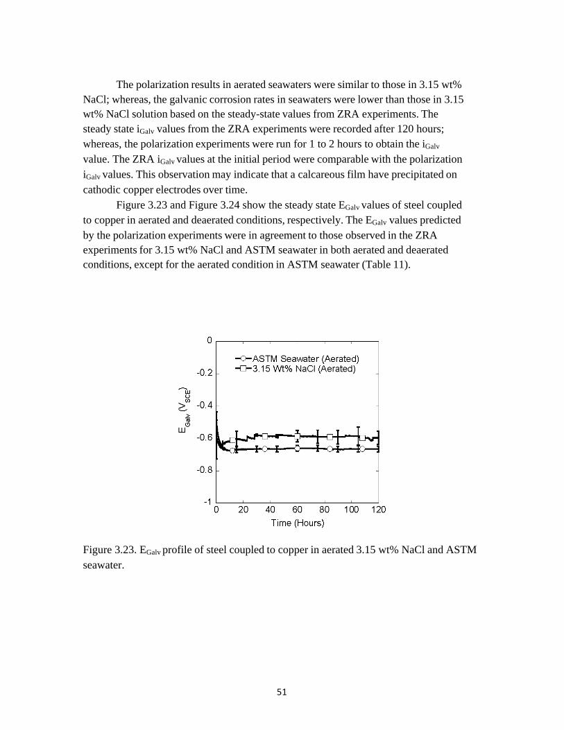
Figure 3.23 and Figure 3.24 show the steady state EGalv values of steel coupled to copper in aerated and deaerated conditions, respectively. The EGalv values predicted by the polarization experiments were in agreement to those observed in the ZRA experiments for 3.15 wt% NaCl and ASTM seawater in both aerated and deaerated conditions, except for the aerated condition in ASTM seawater (Table 11).
Figure 3.23. EGalv profile of steel coupled to copper in aerated 3.15 wt% NaCl and ASTM seawater.

52
Figure 3.24. EGalv profile of steel coupled to copper in deaerated 3.15 wt% NaCl and ASTM seawater.
Table 11. The EGalv (VSCE) values from polarization and short-term ZRA experiments
ASTM Seawater (Deaerated)
ASTM Seawater (Aerated)
3.15 Wt% NaCl (Deaerated)
3.15 Wt% (Aerated)
Polarization -0.756 -0.575 -0.749 -0.569
Short-term ZRA
-0.767
-0.666
-0.756
-0.597
3.4.4 Real Seawater ZRA experiments
The galvanic current between steel and copper in real seawater under immersed
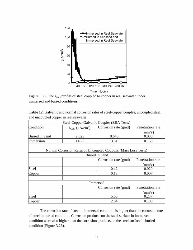
and buried conditions is shown in Figure 3.25. The long-term ZRA experiments were run for 14 days (336 hours). The steady state igalv values in immersed and buried conditions were 14.25 and 2.62 µA/cm2. The iGalv between the electrically connected steel and copper electrodes is related to the rate of the mass loss of the active metal (steel) due to the galvanic effect (Faraday’s law), as shown in equation 4. Corrosion rates in grams per meter squared per day (gmd) were calculated from the steady state iGalv values obtained from the long-term ZRA experiments. The calculated corrosion rates of steel coupled to copper in gmd are shown in the Table 12.
53
Figure 3.25. The iGalv profile of steel coupled to copper in real seawater under immersed and buried conditions. Table 12. Galvanic and normal corrosion rates of steel-copper couples, uncoupled steel, and uncoupled copper in real seawater.
Steel-Copper Galvanic Couples (ZRA Tests) Condition iGalv (µA/cm2) Corrosion rate (gmd) Penetration rate
(mm/y) Buried in Sand 2.625 0.646 0.030 Immersion 14.25 3.51 0.163
Normal Corrosion Rates of Uncoupled Coupons (Mass Loss Tests) Buried in Sand
Corrosion rate (gmd) Penetration rate (mm/y)
Steel 0.42 0.020 Copper 0.18 0.007
Immersed Corrosion rate (gmd) Penetration rate
(mm/y) Steel 5.06 0.237 Copper 2.64 0.108
The corrosion rate of steel in immersed condition is higher than the corrosion rate of steel in buried condition. Corrosion products on the steel surface in immersed condition were also higher than the corrosion products on the steel surface in buried condition (Figure 3.26).

54
Figure 3.26. Corrosion products on the steel surface in real seawater under immersed and buried conditions.
The higher corrosion rate in immersed condition was due to higher dissolved oxygen content when compared to the buried condition. The average dissolved oxygen content in immersed condition was 5.9 mg/L whereas the average dissolved oxygen content in buried condition is less than 1 mg/L. The cathodic reaction in immersed condition is oxygen reduction due to the availability of dissolved oxygen; whereas, the cathodic reaction in buried condition is primarily hydrogen evolution due to less/or negligible oxygen. As shown in polarization experiments, the galvanic corrosion of steel coupled to copper is under cathodic control. Hence, the galvanic corrosion in the immersed condition driven by the oxygen reduction was higher than the galvanic corrosion in the buried condition driven by hydrogen evolution. The iGalv values in the immersed condition diminished greatly from the initial values. A similar trend was observed in artificial ASTM seawater ZRA experiments. Like the ASTM seawater, real seawater also contains ions such as calcium and magnesium (Table 2) that resulted in the formation of calcareous deposits on the cathodic sites. SEM and EDXA results on the copper electrode under immersed conditions showed calcium and magnesium deposits (Figure 3.27, Figure 3.28, Table 13).
Note that the penetration rate of the steel electrode due to galvanic corrosion is relatively low at only 0.163 mm/y in the immersed condition (Table 12). This is caused by calcareous deposits on the copper electrode inhibiting oxygen reduction and therefore lowering the galvanic current. The steel electrode, however, has a total corrosion rate equal to the galvanic component plus a local component caused by cathodic reactions occurring on the steel surface. Hence, the total corrosion rate of the steel electrode is likely greater than that reported in Table 12, which only accounts for the galvanic component. The local component could be in the range of the normal corrosion rate of the

55
uncoupled steel coupons (Table 12). The corrosion rates in Table 12 could be used as a first approximation to estimate the degree of corrosion of the DMM. More studies are needed to obtain longer-term corrosion rates.
Figure 3.27. SEM results on the copper electrode under immersed condition in real seawater
Figure 3.28. EDXA results on the copper electrode under immersed condition

56
Table 13. EDXA results on the copper electrode under immersed condition
Element Weight% Atomic% O K 34.33 59.06
Na K 3.25 5.81 Mg K 6.45 5.48 S K 0.37 0.38 Cl K 7.56 5.98 Ca K 14.73 7.16 Fe K 7.79 3.28 Cu K 36.9 12.50
The EGalv values between steel and copper in immersed and buried conditions in real seawater are shown in Figure 3.29. The EGalv values are much more negative in the buried condition due to the lack of dissolved oxygen. The EGalv values from real seawater ZRA experiments did not agree with the EGalv values obtained from artifical seawater ZRA experiments. This could be due to biological activity over a period of time in real seawater.
Figure 3.29. EGalv profile of steel coupled to copper in real seawater under immersed And buried conditions.

57
3.5 Conclusions The OES analysis identified the DMM casings as high-carbon 1069 steel (UNS G10690), and the rotating band was 99.7 % pure copper (UNS C12210). The galvanic corrosion rates predicted by the polarization experiments in aerated 3.15 wt% NaCl were in agreement to those in aerated ASTM seawater. In ZRA experiments, the initial galvanic currents were high and comparable to those determined using the polarization method; however, the galvanic currents diminished with time in real and ASTM seawater when compared to those in 3.15 wt% NaCl solutions. The calcareous deposits on the copper cathode in the aerated seawaters inhibited oxygen reduction resulting in a decrease in the galvanic current with time compared to that in 3.15 wt% NaCl solution where calcareous deposits do not form. The discrepancies in iGalv values from polarization and ZRA experiments suggest that polarization experiments are good at predicting the mechanisms of galvanic corrosion (e.g., cathodic control in this case); whereas, ZRA experiments are more useful in determining the changes in iGalv over a longer period of time.
The real seawater ZRA experiments showed the corrosion rate of steel coupled to copper under the immersed (0.163 mm/y) condition was much higher than those buried a few inches under sand (0.030 mm/y) due to lack of dissolved oxygen in the buried condition. It should be noted that the penetration rate of steel in the immersed condition due to galvanic corrosion does not represent total corrosion rate, which also includes a local component due to cathodic reactions occurring on the steel that cannot be measured by the ZRA technique. The local corrosion rates could be roughly estimated to be equal to the normal corrosion rates of the uncoupled steel coupons. More testing, however, is needed to obtain reliable long-term galvanic, local, and normal corrosion rates.
3.6 References 1. ASTM G15-92. Standard Terminology Related to Corrosion and Corrosion Testing,
Philadelphia, 1992. 2. Hack, H.P., Galvanic Corrosion, ASTM, 1988 3. Uhlig, Herbert H., “Corrosion Handbook”, John Wiley & Sons Inc., 1948. 4. Uhlig, H.H., Corrosion Handbook, John Wiley & Sons Inc., 1948. 5. Hurst Metallurgical Research Laboratory, Inc., Texas 6. Babion, R., “Predicting Galvanic Corrosion Using Electrochemical
Techniques”,NACE, 1976. 7. Lake Products Inc., Co.
58
8. Deslouis, C., Festy D., Gil O. et al., “Characterization of Calcareous Deposits in Artificial Sea Water by Impedance Techniques,” Electrochemica Acta, Vol. 45, 2000, pp.1837-1845.
9. Hartt W, Culberson C, Smith S., “Calcareous deposits on metal surfaces in Seawater - a critical review,” Corrosion, Vol. 40, No.11, 1984, pp.609-618.
10. Mark M. Benjamin, “Water Chemistry”, McGraw-Hill Series, 2002.