record linkage in health data: a simulation study record linkage simulation.pdf · 4.3 simulation...
TRANSCRIPT

CBS | 2014 Record Linkage in Health Data: a simulation study 3
2014 Scientific Paper
Adelaide Ariel (GGZ inGeest)Bart Bakker (Statistics Netherlands, VU University)Mark de Groot (Utrecht University)Gerard van Grootheest (GGZ inGeest, VU University Medical Centre)Jan van der Laan (Statistics Netherlands)Jan Smit (GGZ inGeest, VU University Medical Centre)Bep Verkerk (GGZ inGeest)
Record Linkage in Health Data: a simulation study

CBS | 2014 Record Linkage in Health Data: a simulation study 3
Contents
1. Introduction 41.1 Project background 41.2 Challenges 51.3 Study goals 51.4 Study approach 7
2. Record linkage theory 82.1 Record linkage: an introduction 82.2 Record linkage methods 11
3. Record linkage: a literature review 153.1 Deterministic record linkage 163.2 Probabilistic record linkage 173.3 Privacy-preserving record linkage 193.4 Assessing linkage quality 203.5 Summary 20
4. Record linkage simulation 214.1 Introduction 214.2 Methods 234.3 Simulation results 294.4 Summary of the simulation results 34
5. Conclusions 37
I. Appendix I. Simulation datasets and errors 39
I.1 Simulation datasets 39I.2 Data population 39I.3 Methods for introduction of errors in linkage variables 42
II. Appendix I. Blocking results 45
III. Appendix I. Simulation results for other I. linkage keys 46
References 57
Glossary 62
Authors 63
CBS | 2014 Record Linkage in Health Data: a simulation study 4
1. Introduction
1.1 Project background
Record linkage is becoming more and more common in statistical and academic research. Linking records makes it possible to combine data from different sources to answer research questions that are very difficult to answer using data from just one source. The advantages of combining different sources have been demonstrated by among others Newcombe et al., (1959); Wallgren and Wallgren (2007); and Bakker and Daas (2012). In many situations, record linkage is an efficient way to collect data and can reduce the inconvenience of asking sensitive questions (Fournel et al., 2009; Herings, 1993). The challenge in record linkage is to link records that belong to the same individual from different sources. Missed links lead to the same problems as nonresponse in surveys. If certain groups of individuals are more difficult to link, estimations could be biased. Similarly, incorrect links, defined as combining the information of two different persons into one record, lead to errors that are similar to measurement error (Bakker and Daas, 2012). The quality of linkage procedures and thus the reliability of the datasets are difficult to determine, and this constitutes a major issue in record linkage.
In health research, linkage has become a popular way to combine data, despite the sensitivity of the information and strict regulations for preventing disclosure of information. Biobanks – collections of biomedical samples with medical, genetic and/or genealogic data (see glossary of terms) – can be greatly enriched by linking them to certain registers, for example for assessing the effect of exposures on health outcomes (Pukkala, 2008). The same holds for longitudinal cohort health data, i.e. information about particular groups of persons. In the Netherlands, many high-quality medical and socioeconomic registers, covering more general population groups, are available for linkage to biobanks and cohorts (Bakker, 2002). The potential of record linkage in health research has been extensively demonstrated (Vink et al., 2006; Eussen et al., 2010; Bozkurt et al., 2009; Schelleman et al., 2006; Bergman et al., 2000). For example, linkage of the Netherlands Cancer Register to the nationwide Dutch Pathology database (PALGA) has been proven to be useful to study the risk and prognosis of endometrial cancer after treatment with tamoxifen (Bergman et al., 2000). Also, linking pharmacy records to biobanks has provided an opportunity to investigate the interactions between thiazide diuretics and genetic variation in the renin-angiotensin-system on the risk of type 2 diabetes mellitus (Bozkurt et al., 2009).
In spite of the fact that record linkage has proven its value in research, it is not just a case of simply following a protocol. Researchers who intend to enrich their data with information from another source need to choose an approach that takes into account the available identifying variables in both sources, a linkage algorithm that combines records based on those variables, and all ethical and legal issues involved. In the present paper, we demonstrate the influence that the choice of variables and linkage algorithms has on linkage results, but also the importance of the properties of the data sources.
The current paper was written as part of Biolink NL, one of the so-called rainbow projects funded by the Dutch Biobanking and Biomolecular Resources Research Infrastructure (BBMRI-NL). BBMRI-NL aims to stimulate collaboration and data sharing between research
CBS | 2014 Record Linkage in Health Data: a simulation study 5
institutes (mostly biobanks), building on existing infrastructures, resources and technologies. The Biolink NL project is a combined effort of researchers from a number of academic research institutes and Statistics Netherlands.
1.2 Challenges
In general, universities and research institutes wishing to enrich their data by linking their own source to external data sources face three challenges. Firstly, privacy laws restrict the use of personal identifiers that can be used to identify the same person in different datasets. Research cohorts are not allowed to store the National Identification Number (NIN, in Dutch: Burger Service Nummer, BSN or Citizen Service Number) in any form. Typically, only personal identifiers such as name, date of birth, etc. are available in their data. Data linkage based on NIN requires permission from the authority concerned and is regulated by a strict protocol to warrant confidentiality. However, even when the NIN can be used for linking, many biobanks or cohorts contain individuals without a NIN.
Secondly, as both biobanks and registers are governed by the statutory legal framework, linking them to other registers may be restricted by law. In addition, access to individual medical registers and biobanks is controlled by various parties with different regulations and committees. Some biobanks use an informed consent procedure that allows their data to be linked with other registers, whereas others do not have such an explicit consent procedure.
Thirdly, and this is not only a challenge for universities and research institutes but also for statistical offices, there is an emerging need to assess linkage quality. Linkage quality is seldomly assessed and almost never on a regular basis after implementation of a new or changed linkage procedure. Linkage quality can be determined by means of a validation, typically by comparing the consistency or the plausibility of research variables (also known as content variables, for example disease history, medicine use, etc.) in the linked records, if the access to such variables is not restricted. While such a procedure is legitimate, one should be aware of potential discrepancies between the content variables due to possible differences in definitions. Moreover, if the target population is changed, the validation must be performed again.
Most of the aforementioned challenges apply to biobanks and research institutes, but not to Statistics Netherlands, which has a unique legal position allowing it to use the NIN for linkage purposes. The compilation of social statistics, including health statistics, is largely based on linked register data (Arts et al., 2000b; de Bruin et al., 2003). These linkages are based on the NIN and therefore linkage quality is high, but Statistics Netherlands is still very interested in the further development of linkage methods. Nowadays, big data mean that large volumes of information are becoming available alongside registers and survey data. The possibilities for linking such data are limited, because the number of potential linkage variables is usually small, and unique identifiers are missing. In this respect, the challenge is to develop new linkage methods that take these aspects into account.
1.3 Study goals
The main goal of the present study is to compare the performance of various record linkage methods in health data when only personal identifiers can be used for linkage. The study

CBS | 2014 Record Linkage in Health Data: a simulation study 6
findings will be published into two white papers. The present – first – paper compares the properties of different linkage methods using simulation datasets, while a second report will be published after real datasets have been linked in three or four demonstration projects.
Previous studies have shown that the combination of personal identifiers provides a feasible alternative if a unique identifier such as the NIN is not available (see for example, Van den Brandt et al., 1990a; Pasquali et al., 2010; Meray et al., 2007; Newcombe et al., 1992). The strength of such combinations is determined by the number of identifiers included, as well as their individual discriminative power (Newcombe et al., 1992; Reitsma, 1999). Although it is tempting to increase the power of the linkage key by combining as many identifiers as possible, in practice variable values contain errors and may change in the course of time, leading to discrepancies in the linkage keys. Moreover, some personal information may not be used as a linkage variable because of privacy concerns.
For example, the identifier surname can be a powerful linkage variable. At the same time, this identifier is error-prone and considered highly sensitive, which restricts its usage even when encrypted. In most situations, the use of this identifier requires additional work such as pre-processing in order to reduce any inconsistency due to either spelling variation or typographical errors. Therefore, it is necessary to recognize in which situations surname should be included for linking.
In this study, we investigate the performance of record linkage methods when certain combinations of personal identifiers are used as linkage variables, taking into consideration that these are not error-free. We select a set of identifiers likely to be present in real data. Another aspect affecting linkage success is the size of the data sources involved. For example, linking large datasets may increase the likelihood of linking the wrong records; it is important to take this into account, as this project comprises various sized data sources.
The overall goal of our study is to improve existing record linkage practice, with the following sub goals:1. To identify which combinations of personal identifiers are indispensable to obtain an
acceptable proportion of correct links;2. To compare the performance of deterministic and probabilistic approaches;3. To describe the influence of dataset size and quality on linkage results.
For both practical and privacy-related reasons, we first evaluate record linkage methods using simulated datasets, in which the true links are known. We compare their performance with different combinations of linkage variables, focusing on identifiers commonly available in cohorts and registers. Because in reality very few databases are completely error-free, errors were introduced into the simulation as well.
We intend to apply the same linkage methods to real data and work together with researchers who have more detailed knowledge of the research topic in the near future. Using these real datasets, we plan to identify which population subgroups, if any, are more difficult to link than others, and hence could give rise to selection bias and inaccurate research outcomes. The findings of these linkages will be presented in a separate white paper.

CBS | 2014 Record Linkage in Health Data: a simulation study 7
1.4 Study approach
This paper consists of five chapters. In the following chapter we introduce the basic theory of record linkage methods. Chapter 3 is a short literature review that focuses on record linkage methodology.
Chapter 4 describes in detail how the datasets for linkage simulation were created in such a way that these resemble existing data in biobanks and registers, including specific population characteristics and varying data quality. Subsequently, the performance of different linkage approaches is compared, using these simulated files.
In short, the following steps were taken:
1. Linkage variables selection. We want to link records using identifiers that are highly discriminative when combined and that are commonly available in registers and biobanks. Content-specific variables, such as types of disease, should be used only as optional linkage variables or as a tool to validate the linking results.
2. Dataset simulation. Different registers and biobanks cover different parts of the population. For example, the general population register (in Dutch: Gemeentelijke Basisadministratie personen, GBA) covers the vast majority of the Dutch population, while a specific disease cohort register covers a specific part of the population and does not necessarily reflect the Dutch population. Because of these differences, a particular linkage strategy may work perfectly for a certain type of register (or combination thereof), but might be less suitable for another type. Because our goal is to examine a linkage strategy that can handle different types of registers and biobanks, it is desirable to test the same methodology on various types of data:
− A dataset covering the population in general (such as the GBA) − A dataset covering a specific part of the population (such as specific disease registrations) − A dataset covering a very specific part of the population (such as birth cohort, females,
twins register)
We created simulation datasets that have the properties of the specific datasets proposed above. Chapter 4 describes how, and Appendix I contains more details.
3. Data error simulation. To simulate various degrees of data quality, we introduced errors into the identifiers. For example, the postal code may not be up-to-date and the date of birth may not be always known for non-natives (Arts et al., 2000). Furthermore, we introduced realistic typographical errors (Oberaigner, 2007; Christen and Pudjijono, 2009).
4. Record linkage simulation. We evaluated the chosen linkage methods in a number of scenarios based on both availability and quality of the linking variables, as well as different overlaps between data sources.
The final chapter summarises the conclusions from the simulation study.

CBS | 2014 Record Linkage in Health Data: a simulation study 8
2. Record linkage theory
This chapter describes a number of factors to be considered when data from different sources need to be linked. Following this, we provide the description of deterministic and probabilistic method in more detail.
2.1 Record linkage: an introduction
Biobanks, research, and health care organizations may have information related to the same individual. This information is kept in their records for specific purposes; for example to monitor health progress, or to detect possible side effects of medicine (Herings, 1993), etc. Each database containing these records has been developed independently to serve a certain organization’s specific purpose, and not other purposes. When combined, records from these data sources can provide substantial information about an individual. Two kinds of combined data can be distinguished: those that consist of records on different persons who share the same characteristics, and those that consist of records on the same person. While the former can be achieved by aggregating the records with respect to the relevant characteristics, the latter requires linking these records at a person level. In most health research, linking records at a person level is preferred (Newcombe, 1994; Reitsma, 1999). Record linkage can be defined as combining different records concerning the same person into one record (Fellegi and Sunter, 1969; Newcombe et al., 1959; Winkler, 2006).
The main challenge in record linkage is to establish whether records from different sources concern the same person. If there is no unique identifier across the data sources1), a set of variables (or fields/attributes) that exist in all records can be used to assist in the decision process. The variables used for linking can be referred to as linkage variables, while the set of all these variables together is called a linkage key: every variable provides a piece of information, and together they form certain information about a specific person (or subject, or entity in a more general sense). Note that information provided by the variables is not uniform: some variables render more information (i.e. are more discriminative) than others. Generally, when two records share the same values on their common variables, they probably refer to the same person (Newcombe et al., 1959).
Deterministic and probabilistic record linkage methods, or a combination the two, are the most commonly applied methods in record linkage. In a deterministic approach, every linkage variable used generally has the same level of importance. If they concur, this would suggest that the respective records belong to the same person and this pair can be considered as a link. In practice, a deterministic approach can be implemented less strictly; for example by leaving out some linkage variables deemed less important, or by relaxing the match criteria for certain variables. A probabilistic approach, on the other hand, explicitly signifies that linkage variables vary in both their discriminative power and quality, and hence agreement or disagreement on them should be treated differently. Agreement on a highly discriminative variable will receive a higher weight than other variables, while disagreement on a variable with a low error rate will have a higher penalty. The overall score on this agreement and disagreement indicates whether a record pair can be linked. This feature makes probabilistic
1) Or databases.
CBS | 2014 Record Linkage in Health Data: a simulation study 9
methods, although computationally more complex, more attractive than deterministic ones. In addition to deterministic and probabilistic methods, new techniques are being developed in database and data mining research, such as rule-based record comparison methods (Hernandez and Stolfo, 1995), machine learning (Elfeky et al., 2002), and Bayesian decision model (Verykios et al., 2002).
The choice for a deterministic or a probabilistic approach depends on the availability and quality of linkage variables. For instance, when the variables are of high quality, a deterministic approach is often preferred over probabilistic methods (L.Gu et al., 2003). When a lower data quality is assumed, a probabilistic approach is often chosen (van Herk-Sukel et al., 2012; Herings, 1993; Reitsma, 1999). In practice, particularly when the data size is very large, a combination of deterministic and probabilistic methods will be used. In the following subsections we discuss the selection procedure for linkage variables, potential errors in these variables and privacy considerations.
2.1.1 Choosing linkage variablesDifferent registrations may hold a different set of variables about the same person. These variables can be divided into the following groups.
− Primary variable: a variable that uniquely identifies each person (e.g. NIN); − Personal identifiers: variables related to general information about a person (e.g. name,
date of birth, sex, address, postal code); − Content (research) variables: variables related to specific information about a person (e.g.
types of disease this person has).
If for any reason a primary variable cannot be used as a linkage variable, personal identifiers, and to some extent content variables, will be used as a substitute. Ideally, these variables should be time invariant, be registered using the same definition, and not be correlated, in order to avoid redundancy of information. The use of content variables in combination with personal identifiers is often not preferred, because of privacy issues. For our simulation, we chose a conservative approach and considered identifiers that are commonly available in registrations: surname, date of birth, sex, and postal code.
2.1.2 Errors in linkage variablesTo link records from different data sources, researchers use variables shared by these data sources and establish whether the values in the different data sources that correspond to the same variable match. These variables may be of various types, and each type poses a different challenge. For instance, evaluating similarity between two names requires a different approach than judging similarity of two different time periods. The former may need some knowledge on semantics and morphology, while the latter can be directly observed. The task of evaluating similarity between variables is far from trivial, due to errors or inconsistency in the variables.
In general, linkage variables can be categorized as follows: − String (name, address, postal code, text representations of a date, etc.); − Numeric (age, measurement values such as blood pressure, cholesterol level, etc.); − Categorical (gender, ethnic group, education level, marital status, etc.).
In most situations, the patterns of errors or inconsistencies in the records are specific to the type of variables:
CBS | 2014 Record Linkage in Health Data: a simulation study 10
− String variables could be prone to spelling mistakes. When typing string variables into a registration, various errors may occur: mistakenly added extra strings (insertion), accidently placing the strings in a wrong order (transposition), accidentally removing some characters (deletion), and randomly changing some characters (replacement).
− Numeric variables are more likely to have inconsistencies due to rounding, which is subject to personal preferences especially when there is no explicit convention in writing them.
− Categorical variables were thought to be more rigid as they typically consist of only a short code and hence minimize potential errors in typing them. However, when errors or inconsistencies occur, for example in a situation involving judgment for classification, their effect on misclassifications would be serious.
These errors occur variably, depending on the protocol used in the registration systems, as different registration systems may employ different approaches in how they register, store and update the information. For instance, the same variable may be saved as a numeric type in one system, but as a string in another; surname prefix may be saved separately in one system but saved together with the surname elsewhere; the existence of the postal code is checked upon entry in one system but not in another, etc. Also, they vary by how familiar one is with the inputs: for example, typing unfamiliar names might result in more mistakes than typing familiar names.
All these factors result in significant inconsistency when records from different systems need to be linked. A standardization procedure during the processing stage is usually effective only for certain problems, mostly related to variations in the variable types and, to some extent, typographical errors. For other problems, such as different surname for the same person, different address due to the time-lag, or different criteria for the same disease, these cannot be solved by standardization alone.
Based on all the factors that may cause errors, we distinguish two types of potential errors in linkage variables: random errors and systematic errors.
Random errors. We define random errors as errors that do not depend on the identifier value and may thus occur in any record. How these errors occur, however, is not random. For instance, for string variables it is assumed that most errors arise from the middle position of the string, as people usually tend to type the first characters more carefully (Porter and Winkler, 1997).
Systematic errors. We define systematic errors as errors that are more likely to take place in records with certain values; thus their occurrence does depend on a specific identifier. For instance, typing the name of a foreigner is more likely to result in more errors than typing a familiar name (see Oberaigner, 2007). Likewise, married women may be registered under their maiden name in one registration system and under their partner’s name in the other system. Such inconsistencies are hard to detect.
2.1.3 Privacy considerationsBecause medical files contain sensitive information, it is common practice to separate personal identifying variables from clinical or medical information. Researchers who wish to analyze the linked data receive datasets that do not contain identifying variables.
CBS | 2014 Record Linkage in Health Data: a simulation study 11
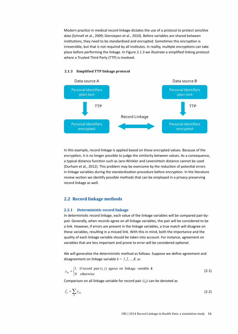
Modern practi ce in medical record linkage dictates the use of a protocol to protect sensiti ve data (Schnell et al., 2009; Giersiepen et al., 2010). Before variables are shared between insti tuti ons, they need to be standardized and encrypted. Someti mes this encrypti on is irreversible, but that is not required by all insti tutes. In reality, multi ple encrypti ons can take place before performing the linkage. In Figure 2.1.3 we illustrate a simplifi ed linking protocol where a Trusted Third Party (TTP) is involved.
Personal Identifiers -‐plain text-‐
Personal Identifiers -‐encrypted-‐
Data source A
TTP
Personal Identifiers -‐plain text-‐
Personal Identifiers -‐encrypted-‐
Data source B
TTP
Record Linkage
In this example, record linkage is applied based on these encrypted values. Because of the encrypti on, it is no longer possible to judge the similarity between values. As a consequence, a typical distance functi on such as Jaro-Winkler and Levenshtein distance cannot be used (Durham et al., 2012). This problem may be overcome by the reducti on of potenti al errors in linkage variables during the standardizati on procedure before encrypti on. In the literature review secti on we identi fy possible methods that can be employed in a privacy preserving record linkage as well.
2.2 Record linkage methods
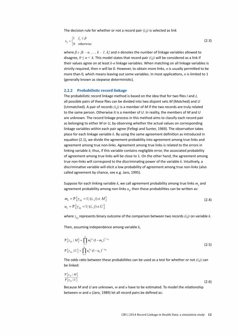
2.2.1 Deterministic record linkageIn deterministi c record linkage, each value of the linkage variables will be compared pair-by-pair. Generally, when records agree on all linkage variables, the pair will be considered to be a link. However, if errors are present in the linkage variables, a true match will disagree on these variables, resulti ng in a missed link. With this in mind, both the importance and the quality of each linkage variable should be taken into account. For instance, agreement on variables that are less important and prone to error will be considered opti onal.
We will generalize the deterministi c method as follows. Suppose we defi ne agreement and disagreement on linkage variable k = 1,2,…,K as
yi, j
kij =1 if record pair ( ) agrees on linkage variable kk0 otherwise
(2.1)
Comparison on all linkage variable for record pair (i,j) can be denoted as
fij kijk
=∑γ (2.2)
2.1.3 Simplified TTP linkage protocol
CBS | 2014 Record Linkage in Health Data: a simulation study 12
The decision rule for whether or not a record pair (i,j) is selected as link
xf
ijij=≥
1
0
β
otherwise
(2.3)
where β ε {k – n, ... , k – 1, k} and n denotes the number of linkage variables allowed to disagree, 0 ≤ n < k. This model states that record pair (i,j) will be considered as a link if their values agree on at least k-n linkage variables. When matching on all linkage variables is strictly required, then n will be 0. However, to obtain more links, n is usually permitted to be more than 0, which means leaving out some variables. In most applications, n is limited to 1 (generally known as stepwise deterministic).
2.2.2 Probabilistic record linkageThe probabilistic record linkage method is based on the idea that for two files I and J, all possible pairs of these files can be divided into two disjoint sets M (Matched) and U (Unmatched). A pair of records (i,j) is a member of M if the two records are truly related to the same person. Otherwise it is a member of U. In reality, the members of M and U are unknown. The record linkage process in this method aims to classify each record pair as belonging to either M or U, by observing whether the actual values on corresponding linkage variables within each pair agree (Fellegi and Sunter, 1969). The observation takes place for each linkage variable k. By using the same agreement definition as introduced in equation (2.1), we divide the agreement probability into agreement among true links and agreement among true non-links. Agreement among true links is related to the errors in linking variable k; thus, if this variable contains negligible error, the associated probability of agreement among true links will be close to 1. On the other hand, the agreement among true non-links will correspond to the discriminating power of the variable k. Intuitively, a discriminative variable will elicit a low probability of agreement among true non-links (also called agreement by chance, see e.g. Jaro, 1995).
Suppose for each linking variable k, we call agreement probability among true links mk and agreement probability among non-links uk, then these probabilities can be written as:
m i j M
u i j U
k kij
k kij
= = ∈{ }= = ∈{ }P | ( , )
P | ( , )
γ
γ
1
1 (2.4)
where γkij represents binary outcome of the comparison between two records (i,j) on variable k.
Then, assuming independence among variable k,
P | ( )
P | ( )
γ
γ
γ γ
γ γ
kij k kk
K
kij k k
M m m
U u u
kij kij
kij
{ } = −
{ } = −
−
=
−
∏ 1
1
1
1
1 kkij
k
K
=∏1
(2.5)
The odds ratio between these probabilities can be used as a test for whether or not (i,j) can be linked:
P |
P |
γ
γkij
kij
M
U{ }{ } (2.6)
Because M and U are unknown, m and u have to be estimated. To model the relationship between m and u (Jaro, 1989) let all record pairs be defined as:
CBS | 2014 Record Linkage in Health Data: a simulation study 13
gM
ij =∈( , )
( , )1 00 1
if record pair (i,j) if record pair (i,,j) ∈
U (2.7)
and suppose the complete data vector can be defined as
G = γ ij ijg, (2.8)
The complete data likelihood involving all record pairs (i,j) can be written as
f m u p pg M p g Uij ij ij iji j
( | , , ) P( | ) ( ) P( | )( , )
G = + −∏ γ γ1
(2.9)
where p represents the proportion of record pairs (i,j) that belong to M, and (1-p) for the proportion of record pairs belong to U, accordingly.
Solving equation (2.9) directly to obtain m, u, and p is impossible, as the values for agreement indicator in equation (2.1) are observable, while the values for the indicator variable in equation (2.7) are unknown. To solve this problem, one can apply an Expected-Maximization (EM) algorithm proposed by Dempster et al. (1977).
An EM algorithm consists of two steps: expectation and maximization steps, which are executed iteratively. It starts by using initial estimates of the parameters: in our case m, u, and p). These initial estimates are used to construct the values of the missing variable (in our case g). This procedure is called the expectation step. Once the values of g have been obtained, they will be used as inputs for equation (2.9) where the new values for m, u, and p will be obtained by maximizing this equation. The whole process is repeated until the estimates for m, u, and p converge. Because this approach is an approximation method, it is advisable to repeat the whole procedure using different values for initial estimates. Jaro (1989) provided practical details on how to obtain g, m, u, and p by using an EM algorithm and argued that the algorithm is relatively stable as long as the initial values for m estimates are higher than those for u estimates. Bauman Jr. (2006) shared his code for the implementation of EM algorithm in SAS.
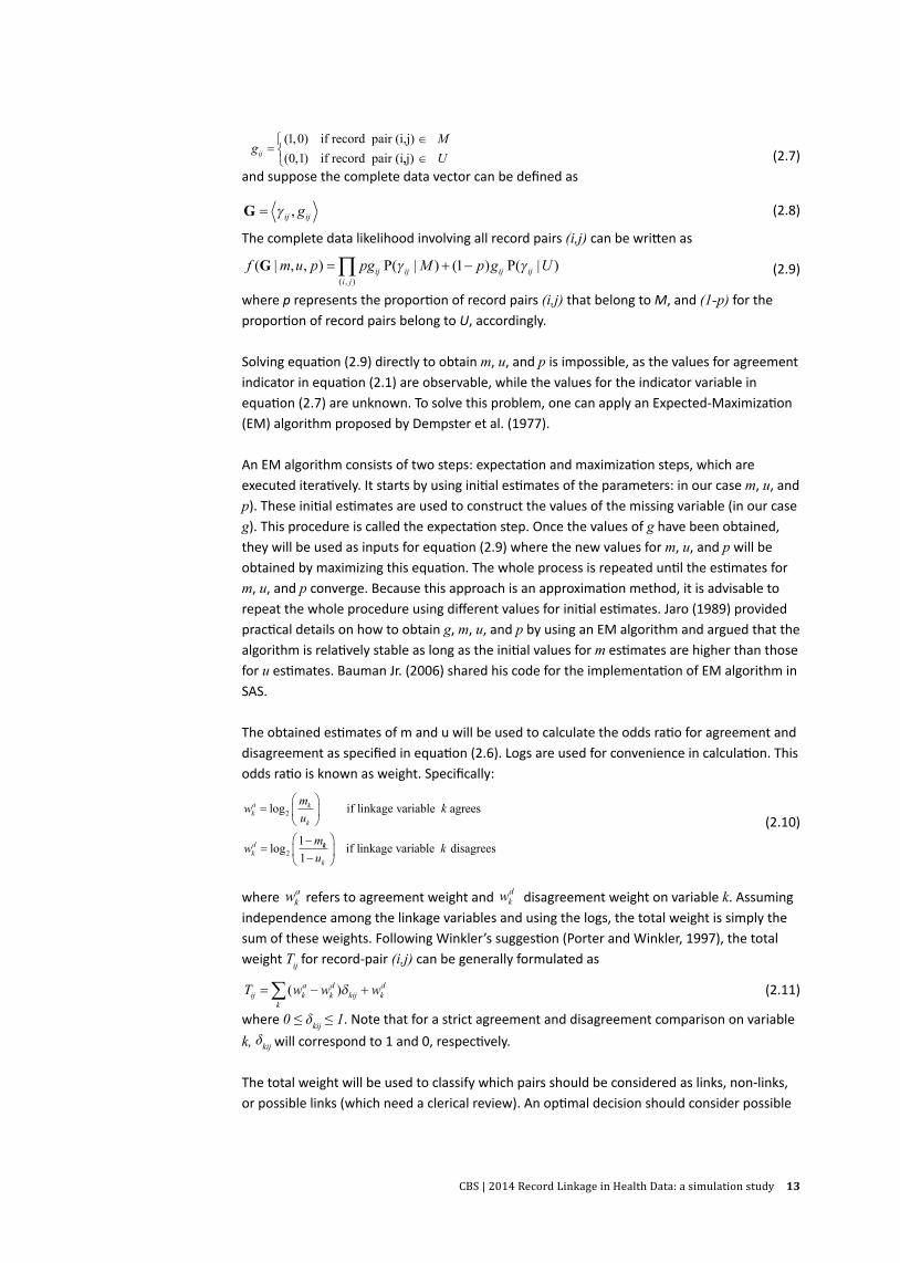
The obtained estimates of m and u will be used to calculate the odds ratio for agreement and disagreement as specified in equation (2.6). Logs are used for convenience in calculation. This odds ratio is known as weight. Specifically:
w mu
k
w m
ka k
k
kd
=
=−
log
log
2
2
1
if linkage variable agrees
kk
kuk
1−
if linkage variable disagrees
(2.10)
where wka refers to agreement weight and wk
d disagreement weight on variable k. Assuming independence among the linkage variables and using the logs, the total weight is simply the sum of these weights. Following Winkler’s suggestion (Porter and Winkler, 1997), the total weight Tij for record-pair (i,j) can be generally formulated as
T w w wij ka
kd
kij kd
k= − +∑ ( )δ
(2.11)
where 0 ≤ δkij ≤ 1. Note that for a strict agreement and disagreement comparison on variable k,
δkij
will correspond to 1 and 0, respectively.
The total weight will be used to classify which pairs should be considered as links, non-links, or possible links (which need a clerical review). An optimal decision should consider possible
CBS | 2014 Record Linkage in Health Data: a simulation study 14
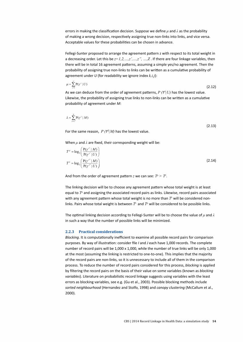
errors in making the classification decision. Suppose we define μ and λ as the probability of making a wrong decision, respectively assigning true non-links into links, and vice versa. Acceptable values for these probabilities can be chosen in advance.
Fellegi-Sunter proposed to arrange the agreement pattern z with respect to its total weight in a decreasing order. Let this be z=1,2,…,z’,…,z’’, …,Z . If there are four linkage variables, then there will be in total 16 agreement patterns, assuming a simple yes/no agreement. Then the probability of assigning true non-links to links can be written as a cumulative probability of agreement under U (for readability we ignore index k,i,j):
µ γ==∑P( | )'
z
z
z
U1 (2.12)
As we can deduce from the order of agreement patterns, P (ϒ1|U) has the lowest value. Likewise, the probability of assigning true links to non-links can be written as a cumulative probability of agreement under M:
λ γ==∑ P( | )
''
z
z z
Z
M
(2.13)For the same reason, P (ϒZ|M) has the lowest value.
When μ and λ are fixed, their corresponding weight will be:
T MU
T MU
z
z
z
z
µ
λ
γγ
γγ
=
=
logP( | )
P( | )
logP( | )
P( | )
'
'
''
''
2
2
(2.14)
And from the order of agreement pattern z we can see: Tμ > Tλ.
The linking decision will be to choose any agreement pattern whose total weight is at least equal to Tμ and assigning the associated record pairs as links. Likewise, record pairs associated with any agreement pattern whose total weight is no more than Tλ will be considered non-links. Pairs whose total weight is between Tλ and Tμ will be considered to be possible links.
The optimal linking decision according to Fellegi-Sunter will be to choose the value of μ and λ in such a way that the number of possible links will be minimized.
2.2.3 Practical considerationsBlocking. It is computationally inefficient to examine all possible record pairs for comparison purposes. By way of illustration: consider file I and J each have 1,000 records. The complete number of record pairs will be 1,000 x 1,000, while the number of true links will be only 1,000 at the most (assuming the linking is restricted to one-to-one). This implies that the majority of the record pairs are non-links, so it is unnecessary to include all of them in the comparison process. To reduce the number of record pairs considered for this process, blocking is applied by filtering the record pairs on the basis of their value on some variables (known as blocking variables). Literature on probabilistic record linkage suggests using variables with the least errors as blocking variables, see e.g. (Gu et al., 2003). Possible blocking methods include sorted neighbourhood (Hernandez and Stolfo, 1998) and canopy clustering (McCallum et al., 2000).
CBS | 2014 Record Linkage in Health Data: a simulation study 15
Matching. In addition to exact matching, similar matching can be incorporated in the weights in the probabilistic approach. In similar matching, the value δkij in equation (2.11) will be between 0 and 1, and will lead to a lower weight if two values of the same linkage variable are similar than if they are exactly the same. The Jaro-Winkler distance method (Porter and Winkler, 1997) is widely used in record linkage to calculate similarity between two strings. Other popular methods are Levenshtein distance (Levenhstein, 1966) and the n-gram method (Churches and Christen, 2004a).
Linking. Alternative methods include the Bayesian decision model, where the cost of making a misclassification is minimized (Verykios et al., 2002) and a mathematical programming model where the total weight is maximized (Jaro, 1989).
SummaryThis chapter has presented a basic and general theoretical background on record linkage. It has explained that the choice of linkage variables is often determined by availability in the data sources and is limited by privacy regulations. Linkage methods include the use of different algorithms, that can be either classified as deterministic or probabilistic. The next chapter reviews the literature on the theory of record linkage in health care settings.
3. Record linkage: a literature review
This section summarizes how deterministic and probabilistic methods are applied in the health data context. A literature review was conducted for this purpose.
As record linkage covers a very broad range of applications – marketing, fraud detection, government administration, healthcare research – the terminology used varies. In order to gain some idea of the terminology, we started by looking for published and unpublished papers that provide an overview of record linkage or a literature review on record linkage. This resulted in papers written by researchers in various fields, ranging from government researchers to university scholars (Silveira and Artmann, 2009; L.Gu et al., 2003; Winkler, 2006).
We used the following terms: ‘record link*’ and (health or epidemi* or cohort) in Web of Knowledge and PiCarta to narrow our search to published papers only2). To take into account the most recent technological developments, we included papers published from 2007 onwards, with some exceptions. We only included papers in which the linkage methods were explained.
As methods and data sources vary considerably, it is difficult to compare the linkage success of different studies. This review aims to identify certain conditions that are required to achieve successful linkage, and to learn how others assessed the correctness of the linkage.
2) The authors wish to thank Caroline Planting and the VUMC library staffs who have helped us searching and finding the papers.
CBS | 2014 Record Linkage in Health Data: a simulation study 16
3.1 Deterministic record linkage
In the deterministic method, all linkage variables used for comparison have the same level of importance. This implies that, generally, agreement on all linkage variables is required to infer that the corresponding pair of records belongs to the same person (a link).
The literature related to the application of the deterministic method suggests that there are two ways to evaluate agreement between linkage variables:
1. Exact matching. Agreement or disagreement is determined by directly observing whether the values of every linkage variable are exactly the same. Generally, this can be done in two ways: fully matching or partial matching. Fully matching uses the complete or full value of the linkage variables; for example, matching on the full surname, the complete date of birth, the complete address. Partial matching, on the other hand, uses only a partial value of the linkage variables, such as a substring of the first four characters of the surname.
2. Similar matching. While exact matching compares the value directly, similar matching compares the value in a less stringent way. It makes use of a number of criteria to judge whether two different values can be considered similar, i.e. whether their difference is still within an acceptable margin.
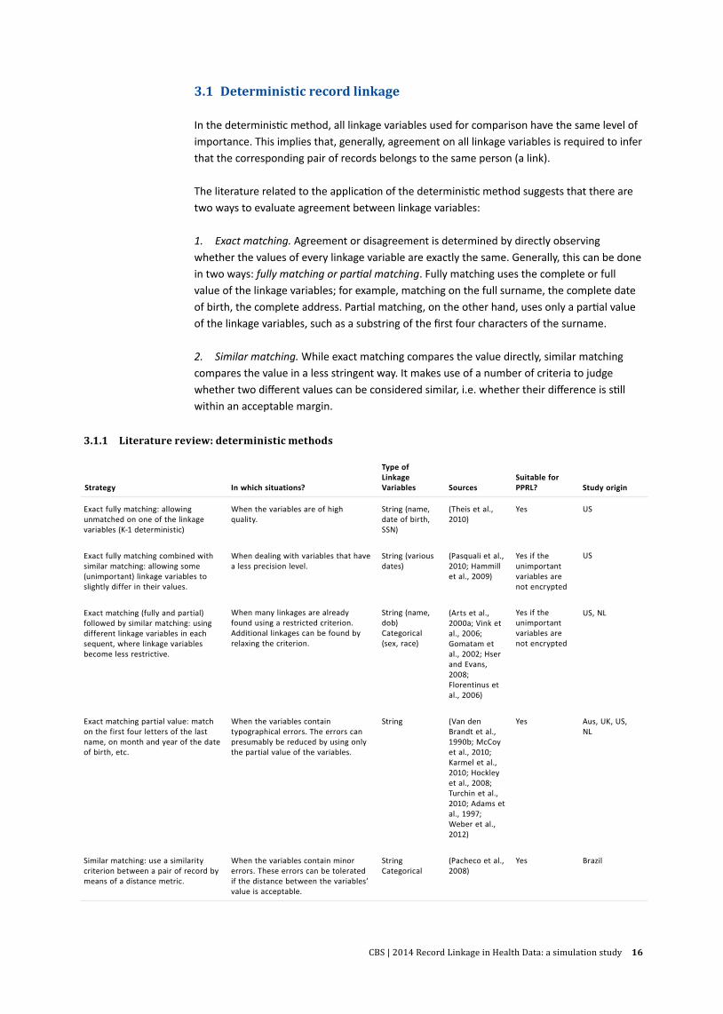
3.1.1 Literature review: deterministic methods
Strategy In which situations?
Type of Linkage Variables Sources
Suitable for PPRL? Study origin
Exact fully matching: allowing unmatched on one of the linkage variables (K-1 deterministic)
When the variables are of high quality.
String (name, date of birth, SSN)
(Theis et al., 2010)
Yes
US
Exact fully matching combined with similar matching: allowing some (unimportant) linkage variables to slightly differ in their values.
When dealing with variables that have a less precision level.
String (various dates)
(Pasquali et al., 2010; Hammill et al., 2009)
Yes if the unimportant variables are not encrypted
US
Exact matching (fully and partial) followed by similar matching: using different linkage variables in each sequent, where linkage variables become less restrictive.
When many linkages are already found using a restricted criterion. Additional linkages can be found by relaxing the criterion.
String (name, dob) Categorical (sex, race)
(Arts et al., 2000a; Vink et al., 2006; Gomatam et al., 2002; Hser and Evans, 2008; Florentinus et al., 2006)
Yes if the unimportant variables are not encrypted
US, NL
Exact matching partial value: match on the first four letters of the last name, on month and year of the date of birth, etc.
When the variables contain typographical errors. The errors can presumably be reduced by using only the partial value of the variables.
String
(Van den Brandt et al., 1990b; McCoy et al., 2010; Karmel et al., 2010; Hockley et al., 2008; Turchin et al., 2010; Adams et al., 1997; Weber et al., 2012)
Yes
Aus, UK, US, NL
Similar matching: use a similarity criterion between a pair of record by means of a distance metric.
When the variables contain minor errors. These errors can be tolerated if the distance between the variables’ value is acceptable.
String Categorical
(Pacheco et al., 2008)
Yes
Brazil

CBS | 2014 Record Linkage in Health Data: a simulation study 17
Most applications of the deterministic method in the reviewed papers apply exact matching, and to a lesser extent, similar matching, simply because exact matching is more convenient as – unlike similar matching – it involves objective judgment. The disadvantage of exact matching, particularly fully matching, is that true links will be missed when there are errors in the linkage variables. Therefore researchers seldom use the deterministic method in just a single run. Instead, they use a stepwise or sequential approach, where either partial matching or similar matching is done in subsequent steps included.
The literature summary is given in Table 3.1.1. We classify and group similar algorithms into one strategy for ease of comparison. Each strategy is case-dependent, which means that it has been proposed to suit a specific problem related to both the availability and the quality of the linkage variables, as well as the size of the datasets. Reporting the linkage results will be less helpful because the datasets and their quality are not the same in these studies. On the other hand, knowing the reasons that researchers chose a particular strategy gives us a fair amount of information to assess whether this strategy will work for the Biolink record linkage. In addition, we also examine whether the strategies will also work in Privacy-preserving record linkage (PPRL).
3.2 Probabilistic record linkage
As opposed to the deterministic method, in the probabilistic method each linkage variable has a certain weight. These weights are determined by the discriminative power and possible errors. The overall weight of the linkage variables is used to decide whether or not a corresponding record pair can be linked, as described in section 2.2.2.
Users of probabilistic methods must take into consideration the following aspects of m and u estimation, weight assignment, and the choice of cut-off value.
Estimation on m and u. The complete data log-likelihood as originally proposed by Dempster et al. (1977) (see equation 2.9 in section 2.2.2) takes all record pairs into account. Because the number of non-links is very dominant, there will be bias in the estimation of m and p. To correct for this, the data log-likelihood should be adjusted to obtain sensible m and p estimates (Yancey, 2002). The literature provides a number of ways to obtain m and u:
1. Using prior information on the probability distribution of the linkage variables as well as the probabilities of different type of error resulting from the record generation process (Fellegi and Sunter, 1969). For example, one can calculate m as equal to one minus the error rate of the identifier, if this is known (Jaro, 1995).
2. Using standard estimation methods, such as expectation maximization (EM) algorithm and maximum likelihood estimation (MLE) (Tromp et al., 2011; Jaro, 1995; Dempster et al., 1977), with some adjustment. Thus, instead of using all record pairs, only the frequency of the patterns will be used (see, e.g., (Tromp et al., 2011; Jaro, 1995)).
3. Using a fuzzy algorithm. For example, by observing the number of agreements, disagreements, and no-decisions (when at least one value is missing) on each linkage variable, for each pair of records selected by a series of random sampling (with replacement) and pairing them as a Cartesian product. The average value of these numbers is used
CBS | 2014 Record Linkage in Health Data: a simulation study 18
to estimate m (in this case m refers to the reliability of the linkage variables) and u (the probability of matching by chance) (Victor and Mera, 2001).
Weight assignment. The weights are calculated as described in section 2.2.2, with some alteration to deal with missing data. For example, Tromp et al. (2006) do not apply a penalty for a variable whose value is missing. Instead, they give no weight value as no decision concerning agreement or disagreement can be made.
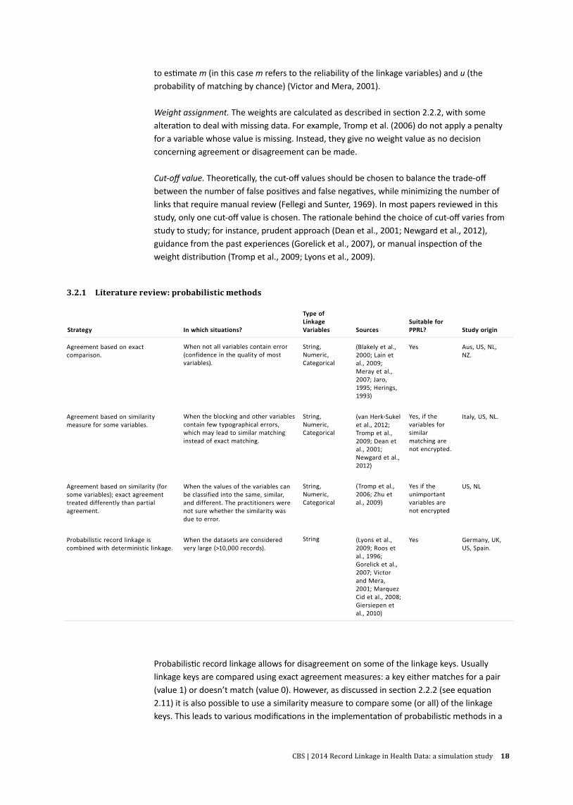
Cut-off value. Theoretically, the cut-off values should be chosen to balance the trade-off between the number of false positives and false negatives, while minimizing the number of links that require manual review (Fellegi and Sunter, 1969). In most papers reviewed in this study, only one cut-off value is chosen. The rationale behind the choice of cut-off varies from study to study; for instance, prudent approach (Dean et al., 2001; Newgard et al., 2012), guidance from the past experiences (Gorelick et al., 2007), or manual inspection of the weight distribution (Tromp et al., 2009; Lyons et al., 2009).
Probabilistic record linkage allows for disagreement on some of the linkage keys. Usually linkage keys are compared using exact agreement measures: a key either matches for a pair (value 1) or doesn’t match (value 0). However, as discussed in section 2.2.2 (see equation 2.11) it is also possible to use a similarity measure to compare some (or all) of the linkage keys. This leads to various modifications in the implementation of probabilistic methods in a
3.2.1 Literature review: probabilistic methods
Strategy In which situations?
Type of Linkage Variables Sources
Suitable for PPRL? Study origin
Agreement based on exact comparison.
When not all variables contain error (confidence in the quality of most variables).
String, Numeric, Categorical
(Blakely et al., 2000; Lain et al., 2009; Meray et al., 2007; Jaro, 1995; Herings, 1993)
Yes
Aus, US, NL, NZ.
Agreement based on similarity measure for some variables.
When the blocking and other variables contain few typographical errors, which may lead to similar matching instead of exact matching.
String, Numeric, Categorical
(van Herk-Sukel et al., 2012; Tromp et al., 2009; Dean et al., 2001; Newgard et al., 2012)
Yes, if the variables for similar matching are not encrypted.
Italy, US, NL.
Agreement based on similarity (for some variables); exact agreement treated differently than partial agreement.
When the values of the variables can be classified into the same, similar, and different. The practitioners were not sure whether the similarity was due to error.
String, Numeric, Categorical
(Tromp et al., 2006; Zhu et al., 2009)
Yes if the unimportant variables are not encrypted
US, NL
Probabilistic record linkage is combined with deterministic linkage.
When the datasets are considered very large (>10,000 records).
String
(Lyons et al., 2009; Roos et al., 1996; Gorelick et al., 2007; Victor and Mera, 2001; Marquez Cid et al., 2008; Giersiepen et al., 2010)
Yes
Germany, UK, US, Spain.
CBS | 2014 Record Linkage in Health Data: a simulation study 19
number of papers, mostly to accommodate specific problems faced during implementation. We summarize our review on the application of probabilistic methods in table 3.2.1. In this table, the first three strategies describe different ways of handling similarity measures in probabilistic linkage. The fourth combines deterministic linkage (which requires exact matching) with probabilistic linkage.
3.3 Privacy-preserving record linkage
In privacy-preserving record linkage, the original values of linkage variables are not revealed during linkage, as both data sources encrypt their variables beforehand. If variables in both data sources are consistent and error-free, the encrypted values concerning the same person will also be the same. However, it is difficult to judge similarity (or close agreement) between two encrypted variables when the original values contain errors.
A number of strategies have been proposed to perform string comparisons in the privacy-preserving environment when the linkage variables contain errors. We summarize them as follows.
− Partial use of linkage variables strategy (Weber et al., 2012). This strategy makes use of part of the linkage variables (e.g. the first four letters of the surname), based on the notion that typographical errors are less likely to occur in the beginning of a string. The encryption takes place on this partial format.
− Phonetic filtering strategy (Quantin et al., 2005; Fournel et al., 2009). This strategy aims to reduce the effect of typographical errors by transforming similar phonetic sounds into the same code. For example, Meijer and Meyer are phonetically similar and are thus assigned the same code. The resulting phonetic codes are encrypted and the comparisons are made on these encrypted values. The Soundex and Metaphone (Karakasidis and Verykios, 2009) algorithm can be used to reduce variations in surnames based on English pronunciation for example.
− n-gram strategy (Durham et al., 2012; Churches and Christen, 2004b; Trepetin, 2008) This method aims to localize the effect of typographical errors by ‘cutting’ a string into a series of n-overlap fragments. In record linkage, bigram or 2-gram is considered sufficient. As an example, the bigrams of Meijer consist of the following elements: _M, me, ei, ij, je, er, r_. Every combination of the elements is encrypted and the similarity between two names is determined by calculating how many bigrams they share. Clearly, such a method requires a huge capacity to store all possible combinations of the n-gram.
− n-gram in combination with bloom filter strategy (Schnell et al., 2009). This approach basically employs the n-gram strategy, but in a compact format, and is considered more secure. In this method, instead of encrypting each combination of the elements separately, independent hash functions are used to encrypt each element and store the results in an array of fragments of a predefined length. All fragments are initialized to 0, and those corresponding to the encrypted element are set to 1. Similarity between two bloom filters is evaluated by comparing them fragment by fragment. It is possible that two different functions map two different elements into the same fragments, thus increasing the likelihood of false links. Kirsch and Mitzenmacher (2008) suggest that two independent hash functions are adequate to minimize the occurrence of false positives.

CBS | 2014 Record Linkage in Health Data: a simulation study 20
3.4 Assessing linkage quality
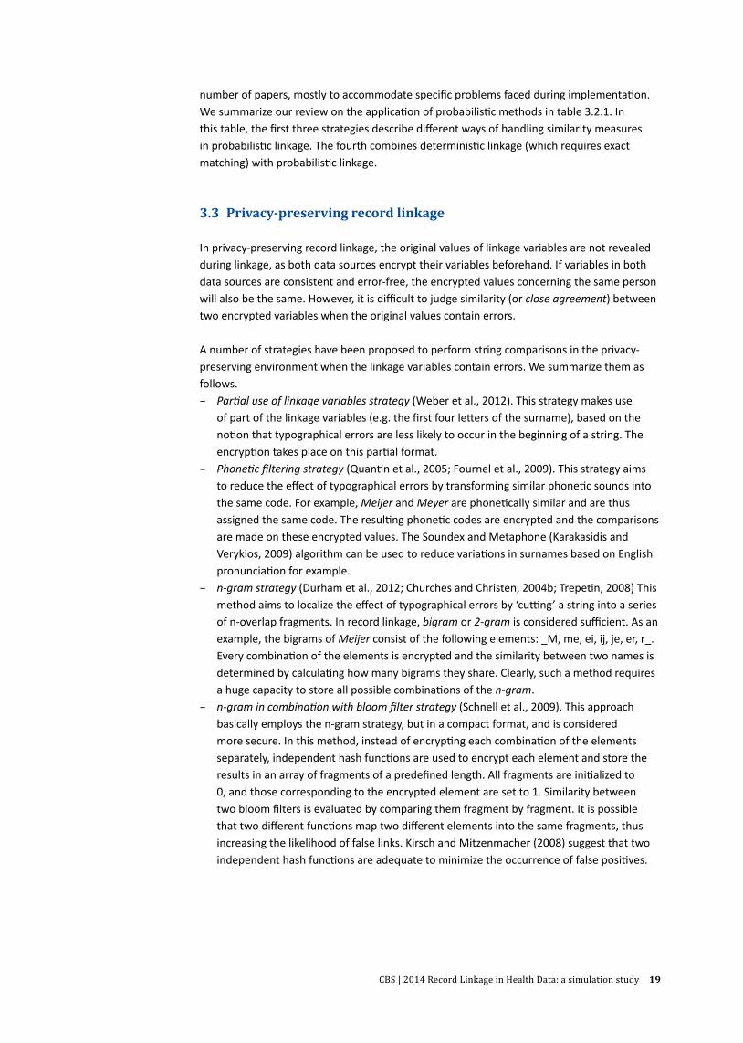
To assess the correctness of the linkage, it is essential to know whether the links obtained actually refer to the same entity, i.e. whether they are true links. If true links are known, the number of false positives (false links) and false negatives (false non-links) can be calculated. Figure 3.4.1 depicts possible combinations between real and observed values.
As in practice real values are often unknown, researchers use an approximation with additional information to infer which links are probably true links. Their approaches vary depending on the quality of their data and the availability of the information. In general, they can be summarized as follows.
− Manual or clerical review (see for example: Karmel et al., 2010; Meray et al., 2007; Victor and Mera, 2001; Zhu et al., 2009; Turchin et al., 2010). This is considered as the gold standard, although it is expensive and time-consuming. Therefore, in practice, only a sample of the linkages are chosen for evaluation.
− With the aid of a sensitive or unique identifier, such as a full name or a Social Service Number (e.g. Weber et al., 2012). These identifiers should be complete and of high quality.
− Comparison using different linkage keys, i.e. cross-validation (see e.g. Lyons et al., 2009; DuVall et al., 2010; Hser and Evans, 2008; Herings, 1993), or using a different linkage method; for example, by comparing the result of deterministic linkage to probabilistic linkage (e.g. Adams et al.,1997). This approach is seen as an inexpensive alternative and there is thus no restriction on the number of links that can be included for evaluation.
In privacy-preserving record linkage, where all linkage variables are encrypted and an access to content variables is prohibited, direct assessment of the linking results is not possible. However, since the occurrences of false positives, and to a lesser extent false negatives, can have a serious effect on the research conclusions, some researchers request permission from the authority to examine the correctness of the linkage using real identifiers (e.g. Weber et al., 2012; Giersiepen et al., 2010).
3.5 Summary
The literature on linkage in health care provides several solutions for the difficulties caused by errors within personal identifiers such as names, birthdates, and addresses. Small variations exist within the deterministic approach, such as exact full matching, partial (substring) exact matching or similar (e.g. phonetic) matching. Probabilistic linkage algorithms make use of weights and cut-off values, which can be varied depending on the situation. In this way,
3.4.1 Real value and possible linking outcomes
Real value
True Link True Non-link
Observation Link True Positive (TP) False Positive (FP)
Non-link False Negative (FN) True Negative (TN)

CBS | 2014 Record Linkage in Health Data: a simulation study 21
researchers are flexible in allowing disagreement between records. Several techniques for both deterministic and probabilistic methods for privacy-preserving record linkage have been described. In the following chapter we use information from this review and describe how the simulation study on record linkage in a health-care setting was performed.
4. Record linkage simulation
4.1 Introduction
The potential for the use of biobanks, registers and health care databases for research can be greatly enhanced by linking them with external data collections. The main purpose of record linkage in health research is to bring together information on individual persons recorded in various data sources. In the previous chapters we have discussed the added value of linkage and the challenges of working with health data, have given a theoretical background, and presented an overview of the literature. Given all these theoretical possibilities for methodological choices, we have tried to investigate and visualise how these choices actually impact linkage in a simulation study. In this chapter, we describe this simulation study to give more insight into the impact of practical choices for linking methodology.
4.1.1 AimWe conducted a simulation of typical applications involving linkage of biobanks and registers without a unique identifier in either data source; unique (universal) identifiers such as national identification numbers (NIN; or in Dutch Burger Service Nummer/BSN) can often not be used as they are intentionally not included or may not be used because of legal restrictions. Other linkage variables must then be selected in combination with an appropriate linkage algorithm. The aim of the simulation study was to compare generic linkage procedures that can be used to link health research data without a unique identifier.
The following sections explain the scope, goal and outcome, and set-up of the simulations. Ideal linkage means that all records in one data source concerning one person are linked to all records in the other data source concerning exactly the same person. At the same time no false positive and no false negative linkages are made. Section 4.2.4 explains in more detail how linkage quality is assessed according to the research question to be studied with the created dataset.
4.1.2 Scope For the purpose of health care research, the result of linking two or more data sources to create enriched datasets depends not only on the nature of the data sources and accuracy of source data, but also on how the properties of the different sources relate to each other. In other words, we can define two properties, because establishing the correct links and discarding the wrong links depend on both (i) the possible combinations and (ii) the ease of detecting or identifying individual persons in a dataset. In this simulation we translate these properties to factors that vary in datasets typically used in ‘real life’ health care research.
CBS | 2014 Record Linkage in Health Data: a simulation study 22
Size influences the number of possible links, either correct or wrong, between data sources. What is the effect of varying source sizes on link quality? And similarly: what is the effect of variation in the degree of shared individuals or overlap between data sources.
The variation in the type of population covered by the data source influences identification of individuals. To illustrate this we created simulation datasets from registers covering the entire Dutch population and registers covering a specific part of the population, such as people with a specific disease, or women treated for fertility problems. The variation in the type of dataset is expected to influence the identification of persons by effects on variability in the linkage keys caused by the selective design (e.g. women, certain age cohorts, frequently moving students, etc.) and availability of linkage keys in the data source. Furthermore, errors in the quality or accuracy of these identifiers caused by things like typing errors, changes of address and name changes through marriage all affect identification.
Within the scope of the simulation, we attempted to cover and address examples of the abovementioned variation by creating dedicated simulation datasets (see 4.2.1). This enabled us to manipulate and investigate the following factors related to these types of datasets and that may pose challenges for linkage: a. Variation in size and type of registration
− Variation in the size of the registrations − Variation in the type of population they cover (i.e., population characteristics);
b. Variation in the proportion of a shared population (overlap);c. Variation in available linkage variables. Datasets differ in terms of the available linkage
variables as a result of differences in design or confidentiality aspects;d. Accuracy of linkage variables. Various errors will be introduced in the datasets to mimic
inaccuracy of data entry and data conversions.
Factors a, b, and d are covered by the creation of a variety of simulation datasets and by the simulation (see 4.1.2) determining which datasets will be linked in the simulations. Factor c is simulated by manipulating the inclusion of linkage variables in the linkage key.
This outline of typical data-related challenges of health care data sources defines the scope of our simulation in terms of variation affecting the data sources. In addition, we provide some guidance on how to perform this linkage.
4.1.3 Deliverables Given the aim and scope described above, the simulation should result in the following deliverables :
1. Development of a linkage strategy that takes into account the variations in health care data sources: differences in size and type, overlap, available linkage variables and accuracy or error level of linkage variables (see 4.1.2).
2. A specific description of a scenario in which no surnames are available as linkage variables, as in reality names may be excluded from datasets for confidentiality reasons.
The simulations will result in linkages showing different performances depending on input and methods that make them more or less suitable for certain research questions. The end product of this whitepaper will be a recommendation that provides guidance to decide on how the ideal linkage should be applied in specific situations, depending on available data sources and research requirements.
CBS | 2014 Record Linkage in Health Data: a simulation study 23
4.1.4 Questions the simulations should answerSumming up the considerations mentioned in the previous sections, the simulation should answer the following questions to serve as input for methodological choices for linking a given combination of datasets:1. Which linking method is suitable given the following variations: size and type of
registrations, possible overlap size, accuracy and error, and exclusion of surname from the linkage key?
2. What choice of linkage key (combination of linkage variables, see 4.2.1) is most appropriate?
4.2 Methods
The methods used for this simulation study are described in terms of the design of the simulation, performance indicators and quality, and the simulation procedure. We start with the design of the simulation to explain what is simulated and what type of data are used. To enable the evaluation of our simulation efforts, our definition of quality of linkage in this whitepaper is elaborated in more detail in section 4.2.4. Lastly in section 4.3 we describe the simulation procedure and the results.
4.2.1 Simulation design In the design of the simulation we explain the creation of datasets, the addition of errors, dimensions or variations to be explored in the simulation, the choice of linkage keys and lastly the algorithms used and their specific applications.
Simulation datasetsTo mimic real life representative electronic health care registers encountered in research linkage, the simulation datasets should vary in size and population coverage.
Therefore, we created the following basic datasets as combinations of size and type: − Large dataset: represents the Dutch population in general (160,000 records) − Medium dataset: represents a specific population group (16,000 records) − Small dataset: represents a more specific population (1,600 records)
To mimic the properties of the various types of datasets, we analysed three existing real life datasets for frequency distributions of sex, names, years of birth, and postal codes (geographical distribution) to construct a blueprint of the dataset types. The frequency distributions were then included in the algorithm to create the simulation datasets. Basic sets containing a unique identifier, surname, date of birth, sex, and postal code, as well as ethnic code, were generated. More details on the creation of simulation datasets are given in Appendix I. No records from any of the abovementioned data sources themselves were included.
The large dataset was based on the characteristics of the ‘general population statistics’ of Statistics Netherlands, obtained from the 2011 figures in StatLine.
The medium dataset was based on the properties of the cancer statistics from the Dutch Cancer Register (in Dutch: Nederlandse Kanker Registratie/NKR). Patients included in this register have been diagnosed with cancer and have been treated by a healthcare professional who reports to this register. As the risk for cancer is age dependent and, for many cancers,

CBS | 2014 Record Linkage in Health Data: a simulation study 24
has a familial or environmental component, age, family names, and addresses may not be randomly distributed.
The small dataset was created based on a blueprint of OMEGA, a female cohort registration based on data from the Dutch fertility clinics in 1996. Variability in the content of linkage variables in this dataset is further restricted as it contains only women.
The first step in creating the basic simulation datasets is illustrated in Figure 4.2.1.1. Within these basic datasets, linkage combination sets, such as small-medium, small-large, and medium-large, were created by adding a different-sized sample from the smallest set of the two to the larger one. Thus in the actual linkage process, records sampled from the smallest set and added to the larger set should be traced back in that combination set. By varying the size of the sample of the smallest set to 10, 60 or 90 percent of the smaller set, we could control the overlap between the datasets.
4.2.1.1 Creation of simulation datasets – steps 1 and 2
10% sample
Fields Id surname date of birth sex postal code
Large (general)
160k
16
k 1.
6k
10% sample
10 % Base set 1.
6k +
160
k 0.
16k
+ 16
k 0.
16k
+ 16
0k
60% sample
Large
Large
60 %
9.6k
+ 1
60k
0.96
k +
16k
0.96
k +
160k
90% sample
90% sample
Large
90 %
14.4
k +
160k
1.
44k
+ 16
k 1.
44k
+ 16
0k
sam
ple
sam
ple
sam
ple
Large Large
Medium Medium Medium
60% sample 90% sample
60% sample 90% sample
10% sample 60% sample 90% sample
Large Large Large
Large Large
Medium (specific)
(general)
Small (very specific)
Step 1Generate basic sets
Step 2Combine sets to create overlap

CBS | 2014 Record Linkage in Health Data: a simulation study 25
Just as in real life, the datasets contain errors. As the precise numbers and types of errors in the real datasets we used for prototyping are unknown, we applied typical errors as mentioned in the literature (Arts et al., 2000; Oberaigner, 2007; Christen and Pudjijono, 2009). We distinguish between random errors that affect linkage variables equally (mostly typographical errors), and systematic errors that occur more often in specific groups. Specifically, we introduced the following errors:
1. Random errors are usually caused by typing errors: inserting a new character, removing a character, replacing a character with another, or wrong placement of a character. For our simulation, these errors translate to minor changes in surname, date of birth, or postal code.
2. Systematic errors occur typically in records with specific values. We assumed the following systematic errors:
– Women of a certain age were more likely to be married and use their partner’s surname;
– Young people and senior citizens were more likely to change their address ; – Non-native people were more likely to have a ‘standard’ or missing date of birth; – Residents of urban areas were more likely to move within their neighbourhood.
Appendix I contains a detailed overview of the types of errors added to records of the simulation sets.
Dimensions explored in simulation Using the simulated datasets, we created a number of possible linking scenarios, which are the combinations of the following factors or dimensions:
− Data source combinations with various sizes and specific types of the population covered. Three combinations between any of the three basic simulation sets were made linking medium (specific) data to large (general) data, small (very specific) data to large data, and small to medium data, or M-L, S-L, and S-M, respectively.
− Overlap size. Three levels of overlap between datasets were defined (small: 10 percent, medium: 60 percent, and large: 90 percent). Samples of 10 percent, 60 percent, and 90 percent (small, medium, large overlap) of the smallest dataset in any combination were drawn and added to the larger dataset.
− Error rates. Three rates – respectively 10 percent, 20 percent, and 30 percent of records with at least one error.
Thus, a possible linking scenario would be: linking small data to medium data, where the overlap size is small and the data have a 10 percent error rate.
Each of three data source combinations (medium-large, small-medium, small-large) will have (3×3) nine unique combinations of overlap level and error rate. As sampling of records for overlap and application of errors are random processes, creating a total of nine simulation sets to cover all combinations of overlap and error size for each data source combination is not sufficient. Therefore, we extend the number of simulation datasets to 40 for each data source combination, which we believe will adequately cover the linking scenarios and the random process.
Choice of linkage keysWe assume that the personal identifiers surname, date of birth, sex and postal code are commonly available in many registrations. However, privacy concerns may prohibit using all of

CBS | 2014 Record Linkage in Health Data: a simulation study 26
them at once, as this could easily lead to disclosure of sensitive personal information. To take into account these real-life restrictions, we need to include this aspect in our simulations. To find smaller subsets of linkage variables that still provide satisfactory linking results, we chose four combinations of three linkage variables and compared their performance with a scenario where all four linkage variables are used:
− all identifiers, versus − surname, date of birth, sex − surname, date of birth, postal code − surname, sex, postal code − sex, date of birth, postal code
Chapter 2 contains a more theoretical discussion of the considerations for linkage variables. It should also be noted that the identifiers are not error-free, and some (e.g. surname) are more error prone than others. We use surnames without their prefixes, which means that people named ‘van den Kamp’ share the same surname as people named ‘Kamp’.
Selection of linking methods and algorithmsLinking health care data requires linking methods that are able to deal with errors in the identifiers and that can ideally also be used with encrypted identifiers, as this is required to comply with privacy requirements. Based on the literature review, the following algorithms are deemed to be capable of handling errors in the identifiers:
1. Deterministic In this linking algorithm, in general all linkage variables should match exactly on content. This simple method has proven to be effective in many situations, especially when data quality is high. In simulations using the linkage variable surname, only the first four characters will be used to reduce the effect of typing errors in this identifier.
2. Probabilistic In these algorithms, every agreement and disagreement on the value of the identifier will receive an agreement weight (reward) and a disagreement weight (penalty) respectively. The net weight determines whether or not the pair should be considered to be a link, a possible link (requiring manual review), or a non-link. The choice of a certain threshold may be subjective. A higher threshold is more stringent, as it will result in more correct links, but at the cost of missing other links (that receive lower weights due to identifier errors). Fellegi-Sunter suggested choosing a threshold in such a way that the number in the category of undetermined ‘possible links’ is minimal (see Chapter 3 for more details).a. Simple probabilistic If ‘surname’ is included for linking, agreement or disagreement on this
identifier will be based on the first four characters of the surname.b. Jaro-Winkler The Jaro-Winkler method calculates the similarity between two names. The
probabilistic method that makes use of Jaro-Winkler will not penalize two names that are not exactly the same; rather, based on their similarity, the respective pair will be assigned a weight that is lower than that assigned for total agreement (i.e. the weight is adjusted to the similarity level). In this simulation, the Jaro-Winkler method is only applicable if surname is included for linking.
c. Bigram Unlike Jaro-Winkler, Bigram does not calculate the similarity between two names. Instead, it cuts a name into a series of two overlapping characters and calculates the shared proportion of these between two names (see Chapter 3 for more details). In this simulation, the Bigram method is only applied if surname is included for linking. In practice, the Bloom filter is used for this method (see 3.3). However, evaluation of Bigram in combination with the Bloom filter is beyond the scope of this simulation, as it requires choices on the hash functions used and filter length.

CBS | 2014 Record Linkage in Health Data: a simulation study 27
The literature finds that Jaro-Winkler is superior for name linkage, but it cannot be applied with encrypted identifiers (Durham et al., 2012). However, it is included here to check how far it outperforms the other methods. The Bigram method does not perform as well as Jaro-Winkler, but it can handle encrypted identifiers. The Bigram method requires a more sophisticated linking protocol, which makes it attractive to check whether the simple probabilistic can do the task and achieve similar results. This would make it an interesting alternative for Bigram.
4.2.2 BlockingBlocking is essential in the probabilistic linking method to enhance computation efficiency. The main goal of blocking is to remove all pairs that are not good candidates for linking (Newcombe et al., 1959). Blocking is applied by filtering the record-pairs on the basis of their value on a number of variables (blocking variables). Although it is desirable to use error-free blocking variables (Fellegi and Sunter, 1969), in most practical situations it is not realistic to expect them to be completely error-free. For this reason, blocking is often applied in a multi-pass way; i.e. other blocking variables are used as a subsequent filter to capture candidate matches missed by initial blocking (variables).
For both practical and fairness considerations, in the simulations we apply the same blocking scheme to all linking scenarios by using only partial value of the identifiers to block. Specifically, we use the combination of the year of birth and the first two digits of the postal code as blocking variables. Our main goal in this case is to obtain a selection for candidate matches that is large enough to enable comparisons between various linking scenarios. With this blocking scheme, the number of pairs for comparison varies from around 8,000 (S-M) to more than 600,000 (M-L), see further details in Appendix II.
For real datasets, it is advisable to use a multi-pass approach for blocking, in order to compensate for the uncertainty in the quality of the blocking variables.
4.2.3 Determinating weight thresholdsIn the probabilistic method, a cut-off value is the minimum weight value required for the record pairs to be classified as a link. A higher cut-off value results in a smaller number of links, and vice versa. Fellegi and Sunter (Fellegi and Sunter, 1969) advised choosing two cut-offs, to distinguish links from possible links and non-links. The cut-offs were selected by balancing the rates of false positives and false negatives in such a way that the number of possible links is minimized. These rates were calculated from the estimated m and u probabilities. However, the estimation of m and u may be susceptible to bias (Jaro, 1995), especially when overlap is small (Fienberg and Manrique-Vallier, 2009). Alternatively, if the true link status is known, the cut-off can be chosen in such a way that the number of false positives and false negatives is minimized (van der Laan, 2013).
In this simulation study, we propose an alternative approach to determine a cut-off value that does not rely directly on the estimation of m and u probability, and that can be applied if the true link status is unknown. Our approach is based on the assumption that the deterministic method will yield mainly correct links, i.e. it has a high precision, but because of errors in the linking variables, it will miss a number of links. The literature suggests that probabilistic methods can cope with errors in the linkage variables, and can thus identify more links (see e.g. Tromp et al., 2006; Dean et al., 2001; Newgard et al., 2012). Our idea is that appropriate weight thresholds can be chosen in such a way that the number of links obtained by probabilistic linkage should equal the number of links obtained by deterministic linkage,
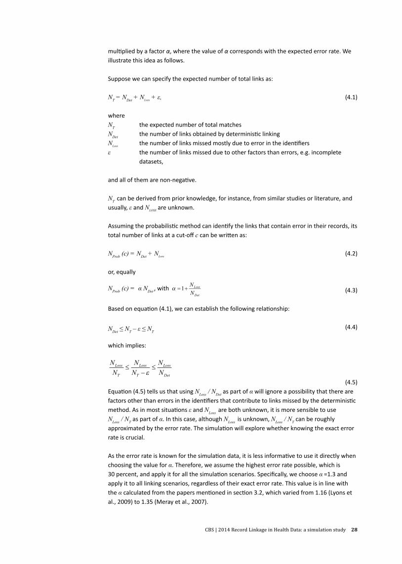
CBS | 2014 Record Linkage in Health Data: a simulation study 28
multiplied by a factor α, where the value of α corresponds with the expected error rate. We illustrate this idea as follows.
Suppose we can specify the expected number of total links as:
NT = NDet + NLoss + ε, (4.1)
whereNT the expected number of total matchesNDet the number of links obtained by deterministic linkingNLoss the number of links missed mostly due to error in the identifiersε the number of links missed due to other factors than errors, e.g. incomplete datasets,
and all of them are non-negative.
NT can be derived from prior knowledge, for instance, from similar studies or literature, and usually, ε and NLOSS are unknown.
Assuming the probabilistic method can identify the links that contain error in their records, its total number of links at a cut-off c can be written as:
NProb (c) = NDet + NLoss (4.2)
or, equally
NProb (c) = α NDet , with α = +1 NNLoss
Det (4.3)
Based on equation (4.1), we can establish the following relationship:
NDet ≤ NT – ε ≤ NT (4.4)
which implies:
NN
NN
NN
Loss
T
Loss
T
Loss
Det
≤−
≤ε
(4.5)Equation (4.5) tells us that using NLoss / NDet as part of α will ignore a possibility that there are factors other than errors in the identifiers that contribute to links missed by the deterministic method. As in most situations ε and NLoss are both unknown, it is more sensible to use NLoss / NT as part of α. In this case, although NLoss is unknown, NLoss / NT can be roughly approximated by the error rate. The simulation will explore whether knowing the exact error rate is crucial.
As the error rate is known for the simulation data, it is less informative to use it directly when choosing the value for α. Therefore, we assume the highest error rate possible, which is 30 percent, and apply it for all the simulation scenarios. Specifically, we choose α =1.3 and apply it to all linking scenarios, regardless of their exact error rate. This value is in line with the α calculated from the papers mentioned in section 3.2, which varied from 1.16 (Lyons et al., 2009) to 1.35 (Meray et al., 2007).
CBS | 2014 Record Linkage in Health Data: a simulation study 29
It is important to note that the α chosen in this study is quite high. When applied appropriately, the deterministic linkage method can still identify links whose records contain some minor error, which implies that in a real situation, a reasonable value for α would be lower than 1 plus the error rate. Nevertheless, our main motivation for choosing a relatively high value for α is to observe to what extent such a value is applicable or is justified across all possible linking scenarios covered in our simulation. This information can be particularly useful if the error rate is unknown.
4.2.4 Performance indicators and quality criteriaIn this simulation, we use precision and sensitivity as performance indicators. Precision is defined as the proportion of correct links found in the linkage divided by the total number of links obtained. Sensitivity is defined as the ratio between correct links and the total number of true links in the dataset.
In terms of quality, we aim to achieve the highest precision and highest sensitivity possible. In practice, high precision corresponds with lower sensitivity, and vice versa. The optimal balance depends on the specific research application for which the linkage is performed. In this simulation, we report both precision and sensitivity without giving rigid guidance on which weighs heavier.
4.3 Simulation results
The simulation results will be presented as follows:1. First, the effect of the threshold on linkage performance will be investigated in section
4.3.1. 2. Next, the cut-off will be set as described previously, and the effect of overlap, linkage
method and error rate on the performance will be investigated in section 4.3.2.3. Section 4.3.3 summarizes the performance of linking methods, given the data source
combination, overlap size, and available linkage variables, mostly because these factors are observable. Thus we hope to come up with a linking strategy based on these factors.
4.3.1 Varying the cut-off values In the probabilistic linking method, the number of links obtained depends on the cut-off value used as the threshold. The higher the cut-off value, the smaller the number of links obtained, as only record pairs with a higher weight value will be selected as links. Record pairs with a high weight value are more likely to be true links, and accordingly, those with a low weight value are least likely to be true links. However, although selecting only pairs with the highest weight value would be a reasonable option, as this would result in a virtually non-existent number of false links, this might exclude correct links that, because of errors or inconsistencies in their attributes or variables, receive a lower weight than they should. Fewer cases for analysis because of false negatives or missed links could cause bias (Tromp et al., 2009). Therefore, in practice researchers attempt to optimize the trade-off between the number of additional links and the respective number of possible false links (see e.g. Karmel et al., 2010).

CBS | 2014 Record Linkage in Health Data: a simulation study 30
4.3.1.1 The number of total links obtained at each cut-off divided by the number of total links obtained by 4.3.1.1 deterministic linkage (i.e., α)
data[[xvar]][sel]
data
[[yva
r]][s
el]
S−M
100
120
140
160
180
200
data[[xvar]][sel]
data
[[yva
r]][s
el]
S−L
data[[xvar]][sel]
data
[[yva
r]][s
el]
M−L
0.1
data[[xvar]][sel]
data
[[yva
r]][s
el]
100
120
140
160
180
200
data[[xvar]][sel]
data
[[yva
r]][s
el]
data[[xvar]][sel]
data
[[yva
r]][s
el]
0.6
data[[xvar]][sel]
data
[[yva
r]][s
el]
0 5 10 15 20 25
100
120
140
160
180
200
data[[xvar]][sel]
data
[[yva
r]][s
el]
0 5 10 15 20 25
data[[xvar]][sel]
data
[[yva
r]][s
el]
0 5 10 15 20 25
0.9
Cut−off
Num
ber o
f lin
ks /
num
ber o
f lin
ks d
eter
min
istic
met
hod
(%)
Ove
rlap
Datasets
DeterministicProb.Simple
Prob.JaroProb.Bigram
α= 1.3 α= 1.3 α= 1.3
α= 1.3 α= 1.3 α= 1.3
α= 1.3 α= 1.3 α= 1.3
data[[xvar]][sel]
data
[[yva
r]][s
el]
S−M
20
40
60
80
100
data[[xvar]][sel]
data
[[yva
r]][s
el]
S−L
data[[xvar]][sel]
data
[[yva
r]][s
el]
M−L
0.1
data[[xvar]][sel]
data
[[yva
r]][s
el]
20
40
60
80
100
data[[xvar]][sel]
data
[[yva
r]][s
el]
data[[xvar]][sel]
data
[[yva
r]][s
el]
0.6
data[[xvar]][sel]
data
[[yva
r]][s
el]
0 5 10 15 20 25
20
40
60
80
100
data[[xvar]][sel]
data
[[yva
r]][s
el]
0 5 10 15 20 25
data[[xvar]][sel]
data
[[yva
r]][s
el]
0 5 10 15 20 25
0.9
Cut−off
Prec
isio
n (%
)
Ove
rlap
Datasets
DeterministicProb.Simple
Prob.JaroProb.Bigram
4.3.1.2 The average precision at different cut-off values

CBS | 2014 Record Linkage in Health Data: a simulation study 31
We start by observing the weight distribution. Although this information is usually displayed in a histogram, we choose to plot a series of cut-off values against the respective number of retrieved links. We do this by plotting the number of retrieved links obtained by probabilistic methods divided by the number obtained by deterministic ones (i.e. we plot α obtained at each cut-off value or α[c]). The results are shown in Figure 4.3.1.1. Subsequently, we plot the corresponding precision and sensitivity values, which are presented in Figures 4.3.1.2 and 4.3.1.3, respectively. In these figures, only the results obtained by using all identifiers are reported. For the other linkage keys, the results are presented in Appendix III.
Based on the results presented in Figure 4.3.1.1, we observe the following: − The effect of overlap size. The results suggest a strong correlation between overlap size
and variations in the values of α in the linking methods, particularly at lower cut-off values. The smallest overlap, in this case 10 percent, gives the largest variations. This is because retrieved links at lower cut-off values are strongly dominated by record pairs that share only partial values on some identifiers. When the overlap size is largest, 90 percent, the variations practically disappear.
− The effect of data source combination. A weaker correlation is found between variations in the number of retrieved links and data source combination. We see in Figure 4.3.1.1 that the variation is less pronounced for small datasets linked with moderate sized datasets (S-M), even at lower cut-off values. This is because the number of pairs – and therefore also the number of possible links – strongly depends on the size of the datasets.
− The effect of error rate. The variation in the number of retrieved links correlates least with the error rate (results not shown). This means there is still a large variation at lower cut-
4.3.1.3 The average sensitivity at different cut-off values
data[[xvar]][sel]
data
[[yva
r]][s
el]
S−M
60
70
80
90
100
data[[xvar]][sel]
data
[[yva
r]][s
el]
S−L
data[[xvar]][sel]
data
[[yva
r]][s
el]
M−L
0.1
data[[xvar]][sel]
data
[[yva
r]][s
el]
60
70
80
90
100
data[[xvar]][sel]
data
[[yva
r]][s
el]
data[[xvar]][sel]
data
[[yva
r]][s
el]
0.6
data[[xvar]][sel]
data
[[yva
r]][s
el]
0 5 10 15 20 25
60
70
80
90
100
data[[xvar]][sel]
data
[[yva
r]][s
el]
0 5 10 15 20 25
data[[xvar]][sel]
data
[[yva
r]][s
el]
0 5 10 15 20 25
0.9
Cut−off
Sens
itivi
ty (%
)
Ove
rlap
Datasets
DeterministicProb.Simple
Prob.JaroProb.Bigram
CBS | 2014 Record Linkage in Health Data: a simulation study 32
offs, regardless of the error rate. We presume that the simulated error rates, in our case up to 30 percent, are not large enough to result in noticeable differences in the patterns.
− The effect of linkage key. The results shown in Figure 4.3.1.1 are based on use of all identifiers for linking. If only a subset of identifiers is used (see results in Appendix III), we still observe the same patterns shown in Figure 4.3.1.1, but only for the combination of surname-date of birth-postal code, and date of birth-sex-postal code.
Furthermore, the pattern of the number of retrieved links is in accordance with the precision. Based on the assumption that the number of retrieved links usually corresponds to precision, we would expect from Figure 4.3.1.1, for instance, that in the case of a small overlap and linked datasets with at least 16,000 records each (M-L), a cut-off value close to 15 should lead to a relatively high precision. Lastly, the number of retrieved links is less likely to correspond to sensitivity. The results in Figure 4.3.1.3 indicate that overall sensitivity patterns are not greatly influenced by overlap size and data source combination. This suggests that it would be less straightforward to detect the sensitivity level based on the number of retrieved links alone.
Conclusion. As these figures indicate, a large overlap will be less problematical than a small overlap, in the sense that high precision is less probable with a small overlap than with large overlap. In addition, the results suggest that plotting the α would help us detect a possible overlap size. Figure 4.3.1.1 shows that when the overlap is the largest, the value of α is less than 1.3, which implies that even though α is fixed at 1.3, the number of additional links obtained by probabilistic methods will be less than 30 percent. In other words, a relatively high α will not affect the performance of the probabilistic methods if the overlap is large, which suggests that it is not necessary to know the error rate beforehand and thus in this case, a high value of α can be chosen. This is not the case for the smallest overlap. In the following section we discuss the implication of choosing such a value for α.
4.3.2 Setting the cut-off valueThis section discusses the precision and sensitivity with respect to the error rate when α = 1.3 is applied for the cut-off, regardless of the overlap size, data source combination and error rate. We aim to investigate when such a choice is justified. Figures 4.3.2.1 and 4.3.2.2 show precision and sensitivity respectively, specified for each error rate.
− Effect of overlap size. When the overlap size is the smallest (in our case 10 percent), as shown in Figure 4.3.1.1 the number of retrieved links fluctuates greatly between the linking methods. As a result, applying the same value of α would also lead to differences in the precision level between the linking methods when the overlap size is small. For the simple probabilistic method, this gives a precision close to that of the deterministic method, while for Jaro-Winkler and Bigram, it results in a much lower precision, especially when the error rate is the smallest. We suspect this occurs because the deterministic method performs very well when the error rate is low. Because Jaro-Winkler and Bigram provide a higher number of retrieved links than the simple probabilistic method, this would also increase the probability of false links. When the overlap size increases, all probabilistic linking methods perform much better than the deterministic linking method.
− Effect of data source combination. Linkage of relatively small datasets (in our case a small dataset linked to a medium-sized dataset, S-M) poses less of a challenge than linkage of large datasets. For the latter case, it would be more likely to increase the number of false positives, particularly in combination with small overlap size.
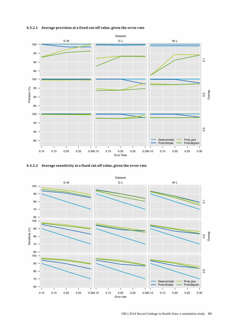
CBS | 2014 Record Linkage in Health Data: a simulation study 33
4.3.2.1 Average precision at a fixed cut-off value, given the error rate
data[[xvar]][sel]
data
[[yva
r]][s
el]
S−M
85
90
95
100
data[[xvar]][sel]
data
[[yva
r]][s
el]
S−L
data[[xvar]][sel]
data
[[yva
r]][s
el]
M−L
0.1
data[[xvar]][sel]
data
[[yva
r]][s
el]
85
90
95
100
data[[xvar]][sel]
data
[[yva
r]][s
el]
data[[xvar]][sel]
data
[[yva
r]][s
el]
0.6
data[[xvar]][sel]
data
[[yva
r]][s
el]
0.10 0.15 0.20 0.25 0.30
85
90
95
100
data[[xvar]][sel]
data
[[yva
r]][s
el]
0.10 0.15 0.20 0.25 0.30
data[[xvar]][sel]
data
[[yva
r]][s
el]
0.10 0.15 0.20 0.25 0.30
0.9
Error Rate
Prec
isio
n (%
)
Ove
rlap
Datasets
DeterministicProb.Simple
Prob.JaroProb.Bigram
4.3.2.2 Average sensitivity at a fixed cut-off value, given the error rate
data[[xvar]][sel]
data
[[yva
r]][s
el]
S−M
60
70
80
90
100
data[[xvar]][sel]
data
[[yva
r]][s
el]
S−L
data[[xvar]][sel]
data
[[yva
r]][s
el]
M−L
0.1
data[[xvar]][sel]
data
[[yva
r]][s
el]
60
70
80
90
100
data[[xvar]][sel]
data
[[yva
r]][s
el]
data[[xvar]][sel]
data
[[yva
r]][s
el]
0.6
data[[xvar]][sel]
data
[[yva
r]][s
el]
0.10 0.15 0.20 0.25 0.30
60
70
80
90
100
data[[xvar]][sel]
data
[[yva
r]][s
el]
0.10 0.15 0.20 0.25 0.30
data[[xvar]][sel]
data
[[yva
r]][s
el]
0.10 0.15 0.20 0.25 0.30
0.9
Error rate
Sens
itivi
ty (%
)
Ove
rlap
Datasets
DeterministicProb.Simple
Prob.JaroProb.Bigram

CBS | 2014 Record Linkage in Health Data: a simulation study 34
− Effect of error rate. As we see in Figures 4.3.2.1 and 4.3.2.2, the performance of the deterministic method is in line with the level of error. This confirms the notion that the deterministic method is the most appropriate for linking high quality data (in this case small error numbers in the linking variables). In such situations, applying probabilistic methods would not lead to significant improvement. In fact, especially when both overlap size and error rates are relatively small (in this case 10 percent), the deterministic method is able to achieve high precision and sensitivity. As sensitivity is already high, using probabilistic methods by setting α=1.3 would be less effective as it might give additional links that would be mostly incorrect. This can be resolved by lowering the predefined value allowed for the maximum number of additional links (α would be less than 1.3), which implies that both the deterministic and probabilistic method would yield a similar number of links. On the other hand, probabilistic methods are more capable in terms of dealing with high error rates than the deterministic method, especially when the overlap is large.
− Effect of linkage key. If not all identifiers are used for linking, the deterministic method is still able to maintain high precision, as opposed to probabilistic methods. Specifically, the combinations name-date of birth-postal code and date of birth-sex-postal code would yield similar precision to when all identifiers are used for linking, and are even able to improve sensitivity. (See Appendix III for the figures.)
Conclusion. The deterministic linking method seems to be the safest choice when overlap is small and the error rate is expected to be small. Probabilistic methods can effectively deal with high error rate, but only when the overlap is large. One possible explanation for this is that in the case of a large overlap, any link identified by the probabilistic method has a higher chance of being correct than when overlap is small. If the error rate is low, no substantial improvement can be made.
4.4 Summary of the simulation results
In this section we summarize the simulation results. Specifically, we observe to which extent data source combination, overlap size as well as available identifiers for linking influence the performance of the linking methods. For the sake of brevity, we choose precision and sensitivity as the criteria for performance measurement. The average of precision and sensitivity are presented in Figures 4.4.1 and 4.4.2 respectively.
Figures 4.4.1 and 4.4.2 confirm the general expectation that there is a trade-off between precision and sensitivity. On average, the deterministic method provides the highest precision level at the cost of resulting in the lowest sensitivity level. The probabilistic method, on the other hand, is believed to be capable of increasing the sensitivity level, although at the cost of a lower precision level. In our case, in general all probabilistic methods evaluated lead to a slightly lower precision level, but are able to increase the sensitivity level to around 10 percent on average. However, there are certain situations where this is not the case.
Our simulation results indicate that no single method outperforms all others in each of the linking scenarios included in this study. This implies that the choice of linkage method depends on certain linking scenarios. This motivates us to evaluate the performance of the linking methods, based on a number of observable factors: linkage keys, overlap size and data source combination. We discuss these factors in more detail below.

CBS | 2014 Record Linkage in Health Data: a simulation study 35
− The influence of data source combination − Small to medium-sized datasets (S-M): This data source combination appears to be the
easiest case. All linking methods manage to achieve similar precision levels when all identifiers were used. But there are still some differences in performance when not all identifiers were used for linking and the overlap is smallest.
− Small to large datasets (S-L): This data source combination seems to be the most challenging linkage compared to the other types. Even when all identifiers were used for linking, we observe that Jaro-Winkler and Bigram methods underperformed when the overlap is not high (in our simulation to 60 percent).
− Medium to large datasets (M-L): This data source combination shows some similarity with the previous type, but performs less well. The probabilistic linking methods are able obtain high precision close to that obtained by deterministic method when the overlap increases (in this case 60%).
− The influence of overlap size − Small overlap: Generally, the performance of the deterministic method would be less
influenced by overlap size, than that of the probabilistic methods. All probabilistic methods perform poorly when overlap size is small, even when all identifiers are used for linking.
● ● ●●
●● ●
● ●●
●● ●
●
●● ●
●
S−M
707580859095
100 ● ●
●
●
●●●
●
●
●
●●
●
●
●●
●
●
S−L● ●
●
●
●● ●
●
●
●
● ●
●
●
● ●
●
●
M−L
0.1
● ● ● ● ●● ● ●●
●
● ● ●
●
● ● ●
●
707580859095
100 ● ●●
●
●● ●
● ●
●
● ●
●
●
● ●●
● ● ● ●
●
●● ●
● ●
●
●
● ● ●
●
● ●
●
0.6
● ● ● ● ●● ● ●●
●
● ●●
●
● ● ●
●
all ndp nsd nsp sdp
707580859095
100 ● ● ●●
●● ●● ●
●
●
●● ●
●●
●●
all ndp nsd nsp sdp
● ● ●●
●● ●●
●
●
●● ●
●
●
● ●
●
all ndp nsd nsp sdp
0.9
Link key
Prec
isio
n (%
)
Ove
rlap
Datasets
DeterministicProb.Simple
Prob.JaroProb.Bigram
4.4.1 Precision (average), given the linkage key
* All (all identifiers are used for linking), ndp (surname-dob-postal code), nsd (surname-sex-dob), nsp (surname-sex-postal code), and sdp (sex-dob-postal code).

CBS | 2014 Record Linkage in Health Data: a simulation study 36
− Medium and large overlap: When the overlap is relatively large (in this case 60 percent) the probabilistic methods result in a precision level similar to that of the deterministic method, but with a much higher sensitivity level. When the overlap is largest, the precision level of the probabilistic methods is close to that of the deterministic method, while the sensitivity level is greatly improved.
− The influence of linkage keys − All identifiers: When all identifiers are used for linking, we expect to obtain the highest
precision regardless of the linking method used. For the deterministic method, this high precision level is accompanied by a much lower sensitivity level. The probabilistic methods employed in this study yield a precision level close to that of the deterministic method, but with a much higher sensitivity level. The simple probabilistic method gives a precision level slightly lower than that of the deterministic method, followed by Jaro-Winkler and Bigram. The simple probabilistic method has a lower sensitivity level than Jaro-Winkler and Bigram.
− Subset of identifiers: If not all identifiers are used for linking, leaving out the identifier surname would still lead to high precision, but only for the deterministic method. The deterministic method and, to a lesser extent, the simple probabilistic method can handle fewer variables and still provide high precision. However, when the identifier date of birth is excluded for linking, the performance of the deterministic method is poorest. The simple probabilistic method performs poorest when the identifier surname is excluded, except in the situation where only relatively small datasets are linked (in our case at most 16,000 records). On the other hand, the precision level of
4.4.2 Sensitivity (average), given the linkage key*
●●
●●
●
●●
●
●
●
● ● ●●● ● ●
●
S−M
75
80
85
90
95
100
●●
●
●
●
● ●
●
●
●
● ●
●
●
● ●
●
●
S−L
● ●
●
●●
● ●
● ●
●
● ●
●
●● ●
●
●
M−L
0.1
●●
●●
●
● ● ● ● ●
● ●● ●● ●
● ●
75
80
85
90
95
100
●●
●●
●
●
●
●●
●
● ●●
●● ●●
●
●●
●
●●
●●
●●
●
● ●●
●●
● ●
●
0.6
●●
● ●
●
● ● ●● ●
● ●● ●● ●
● ●
all ndp nsd nsp sdp
75
80
85
90
95
100
●●
●●
●
●●
●●
●
● ● ●●
● ●●
●
all ndp nsd nsp sdp
● ●
●
●●
●●
● ●
●
● ●●
●● ●
●
●
all ndp nsd nsp sdp
0.9
Link key
Sens
itivi
ty (%
)
Ove
rlap
Datasets
DeterministicProb.Simple
Prob.JaroProb.Bigram
* All (all identifiers are used for linking), ndp (surname-dob-postal code), nsd (surname-sex-dob), nsp (surname-sex-postal code), and sdp (sex-dob-postal code).
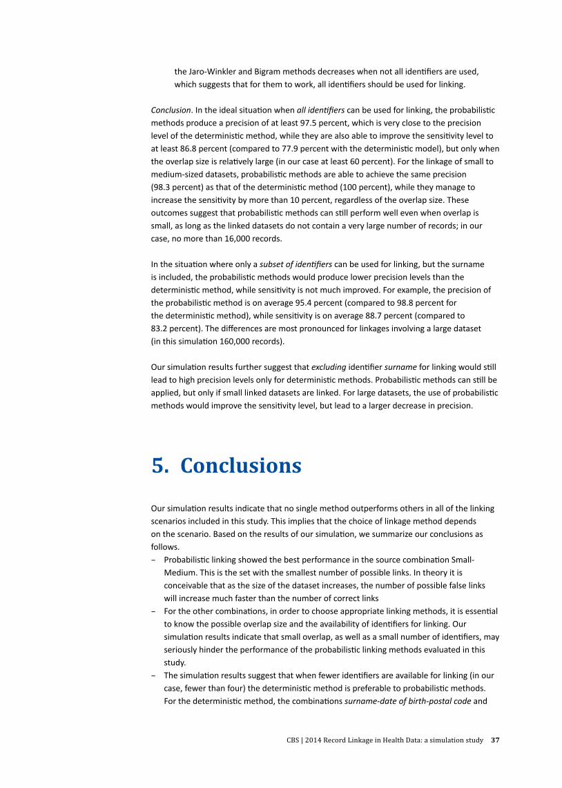
CBS | 2014 Record Linkage in Health Data: a simulation study 37
the Jaro-Winkler and Bigram methods decreases when not all identifiers are used, which suggests that for them to work, all identifiers should be used for linking.
Conclusion. In the ideal situation when all identifiers can be used for linking, the probabilistic methods produce a precision of at least 97.5 percent, which is very close to the precision level of the deterministic method, while they are also able to improve the sensitivity level to at least 86.8 percent (compared to 77.9 percent with the deterministic model), but only when the overlap size is relatively large (in our case at least 60 percent). For the linkage of small to medium-sized datasets, probabilistic methods are able to achieve the same precision (98.3 percent) as that of the deterministic method (100 percent), while they manage to increase the sensitivity by more than 10 percent, regardless of the overlap size. These outcomes suggest that probabilistic methods can still perform well even when overlap is small, as long as the linked datasets do not contain a very large number of records; in our case, no more than 16,000 records.
In the situation where only a subset of identifiers can be used for linking, but the surname is included, the probabilistic methods would produce lower precision levels than the deterministic method, while sensitivity is not much improved. For example, the precision of the probabilistic method is on average 95.4 percent (compared to 98.8 percent for the deterministic method), while sensitivity is on average 88.7 percent (compared to 83.2 percent). The differences are most pronounced for linkages involving a large dataset (in this simulation 160,000 records).
Our simulation results further suggest that excluding identifier surname for linking would still lead to high precision levels only for deterministic methods. Probabilistic methods can still be applied, but only if small linked datasets are linked. For large datasets, the use of probabilistic methods would improve the sensitivity level, but lead to a larger decrease in precision.
5. Conclusions
Our simulation results indicate that no single method outperforms others in all of the linking scenarios included in this study. This implies that the choice of linkage method depends on the scenario. Based on the results of our simulation, we summarize our conclusions as follows.
− Probabilistic linking showed the best performance in the source combination Small-Medium. This is the set with the smallest number of possible links. In theory it is conceivable that as the size of the dataset increases, the number of possible false links will increase much faster than the number of correct links
− For the other combinations, in order to choose appropriate linking methods, it is essential to know the possible overlap size and the availability of identifiers for linking. Our simulation results indicate that small overlap, as well as a small number of identifiers, may seriously hinder the performance of the probabilistic linking methods evaluated in this study.
− The simulation results suggest that when fewer identifiers are available for linking (in our case, fewer than four) the deterministic method is preferable to probabilistic methods. For the deterministic method, the combinations surname-date of birth-postal code and

CBS | 2014 Record Linkage in Health Data: a simulation study 38
date of birth-sex-postal code yield a level of precision similar to when all four identifiers were used. The exclusion of identifier surname in deterministic linking even leads to a higher sensitivity, regardless of data source combination and overlap size. On the other hand, the exclusion of date-of-birth leads to much lower precision, even for large overlap. A possible implication for this is that when the deterministic method is applied in a stepwise manner, where one identifier is relaxed sequentially, it would be better not to relax the date of birth identifier.
− Jaro-Winkler performs slightly better than the Bigram method. Both perform particularly well in situations where overlap is highest (in our case 90 percent), and all identifiers (in our case four) are available for linking. The results suggest that these methods can be applied to improve the performance of the deterministic method (i.e. improving sensitivity), given these conditions.
− The performance of simple probabilistic linkage is similar to Jaro-Winkler and Bigram. In fact, the simple probabilistic method is more effective when the overlap is fairly small (up to 60 percent in this case). The reason Jaro-Winkler does not perform better might be the limited variation in the Dutch names included in our simulated data.
− The application of the proposed method in determining the weight threshold as proposed in section 4.2.3 depends on the overlap. When overlap is small, it is essential to know the exact error rate, and if this information is lacking, it is advisable to choose a rather conservative approach, namely a low value for α. When overlap is large, it is not necessary to know the exact error rate and a high value can be chosen to reflect the possible error rate. Further investigation is needed to assess the effectiveness of this method when real datasets are linked.
The simulation study described here provided useful information about dataset characteristics that influence the performance of different linkage strategies. Nevertheless, real life linkage may not always resemble these controlled circumstances and therefore lead to different conclusions. For example, the error rates of real datasets are usually unknown. Variables may have changed since they were recorded, especially if a database has not been updated for some time. Other differences may result from the greater variation in names that occurs in the population, and certain subgroups may be more difficult to link than the general population. Databases vary greatly in their number of records and certain databases contain a much higher number of records than our simulated datasets. In such situations it may be useful to apply a deterministic linkage first, followed by a probabilistic approach.
Having compared several linkage approaches in a simulated setting where true links are known, the next step is to apply the same linkage methods to real life datasets in which error rates and true links are unknown. We are doing this in a number of demonstration projects that include health care data. These demonstration projects have been chosen in such a way that they differ from each other in terms of population characteristics, time span of data collection, number of records per dataset, and expected overlap between the linked data sources. In a separate white paper we shall describe how each method performs under these different circumstances, and in the end provide a practical guide for researchers who wish to link their data to external registrations.
CBS | 2014 Record Linkage in Health Data: a simulation study 39
I. Appendix I. Simulation datasets and errors
I.1 Simulation datasets
Purpose: to develop simulation datasets that are representative for registers or biobanks involved in the record linkage project Biolink NL.
We assume that the population in a general register covers most of the populations in the other registers. However, while population characteristics in a general register reflect the general population, the population characteristics in the other registers do not necessarily. We specify the population characteristics of the registers based on variations on the following attribute values:
General population characteristics: male-female, a large age interval, and large variations in ethnic groups;Specific population characteristics: male-female, a smaller age interval, and small variations in ethnic groups;Very specific population characteristics: only female, relatively similar age (or a very small age interval), and small variations in
ethnic groups.
Although ethnicity can usually be approximated by surname, this is not always straightforward. For example, people may use their partner’s name, and children usually take their father’s name, while he may belong to a different ethnic group. To resolve this problem, we use surnames not to represent ethnicity per se, but to represent variations in the datasets. For example, when we assume a large variation in ethnic groups, a higher number of unique surnames will be used, while a small variation will be represented by a smaller number of unique surnames. We do identify each record with an ethnicity code (in this case we use only two groups: native and non-native). This code, possibly in combination with other attributes such as sex and age, will be used as a guidance when errors are introduced in the datasets.
I.2 Data population
A pool containing the values of the identifiers will be used to generate simulated datasets. We start by constructing a set of surnames and a set of postal codes that are selected from the real values. Approximately 300,000 unique surnames were present in the municipal database in 2007 (representing a total population of around 16.3 million people), while 470,000 postal codes were in use in 2005 (source of information: Meertens Institute of Genealogy and TNT Post). Rescaling these numbers to adjust for the size of our simulation datasets (with a maximum number of records of around 160,000), we use 3,000 unique most popular Dutch names and 5,000 postal codes. These values serve as a pool for the surnames and postal codes from which we draw the values for the simulation datasets. Postal codes are selected in proportion to the density of the Dutch population.

CBS | 2014 Record Linkage in Health Data: a simulation study 40
The following sections describe in more detail how the datasets are created. The summary will be given in Table I.2.2.
I.2.1 General population characteristicsThe following restrictions are taken into consideration when constructing a dataset reflecting the overall general population:
− Each person is assigned to a household. − A household consists of at least one adult. − A household consisting of at least two persons may have different surnames. − Approximately 37 percent of total households are one-person households (source of
information: household figure 2011 SN). − One postal code will be assigned to 20–25 households (source of information: TNT Post). − A surname can be shared by more than one person. Approximately 10 percent of the total
population share a few surnames. − The ratio between men and women is equal. − The variation in ethnic groups is large (23 percent non-native)
I.2.2 Specific population characteristicsThe following restrictions are taken into consideration when constructing a dataset reflecting a specific population:
− No households are used when generating this dataset. Instead, we use the following information:
− Specific age interval relates to the occurrence of a specific disease − Specific sex relates to the occurrence of a specific disease − Small variation in ethnic groups (10 percent non-native)
I.2.3 Very specific population characteristicsThe following restrictions are taken into consideration when constructing a dataset reflecting a very specific population:
− No households are used when generating this dataset. Instead, we use the following information:
− A small age interval − Only one sex (female) − Small variation in ethnic groups (less than 10 percent non-native)
I.2.4 Simulation dataset sizesFor our simulation, we adjust the size of each dataset proportionally to its original data size, which leads to the following sizes:
− Dataset representing general population: 160,000 (individual) records − Dataset representing specific population: 16,000 (individual) records − Dataset representing a very specific population: 1,600 (individual) records

CBS | 2014 Record Linkage in Health Data: a simulation study 41
I.2.1 Creation of simulation datasets
10% sample
Fields Id surname date of birth sex postal code
Large (general)
160k
16
k 1.
6k
10% sample
10 % Base set
1.6k
+ 1
60k
0.16
k +
16k
0.16
k +
160k
60% sample
Large
Large
60 %
9.6k
+ 1
60k
0.96
k +
16k
0.96
k +
160k
90% sample
90% sample
Large
90 %
14.4
k +
160k
Erro
r lev
els
1.44
k +
16k
1.44
k +
160k
sam
ple
sam
ple
sam
ple
Large Large
Medium Medium Medium
60% sample 90% sample
60% sample 90% sample
10% sample 60% sample 90% sample
Large Large Large
Large Large
Medium (specific)
(general)
Small (very specific)
Step 1 Generate basic sets
Step 2 Combine sets to create overlap
10% sample
10% sample 60% sample
Large
Large
90% sample
90% sample
Large Large
Medium Medium Medium
60% sample 90% sample
60% sample 90% sample
10% sample 60% sample 90% sample
Large Large Large
Large Large
10 % 10 %
20 %
30 %
60 % 90 %
Step 3 Apply three error levels
Step 4 Increase the number of sets
For each linkage type (row):‐Repeat step 2&3 four times (9 sets * 4 repeats=36 sets)‐Add 4 random linkage sets
‐‐> 40 sets per type
I.2.2
Population General Specific Very specific
Sources of information Statline, Meertens Dutch Cancer Register (NKR)
Dutch National CancerInstitute (NKI)
Total number of records created 160,000 16,000 1,600
Unique number of surname (%) 19 30 * 575
Sex (in %) male 501 522 −
female 499 478 100
Ethnicity (in %) native 798 90 .0* 924
non-native 202 10 .0* 76
Age category (in %) 0–20 yr 176 11 0
21–45 yr 429 47 46
46–65 yr 268 354 949
66–80 yr 99 293 04
older than 80 yr 29 294 001
Household type (in %) one-person household 370 n.a n.a
other household 630 n.a n.a
Postal code region (in %) North 106 10 .6* 10 .6*
East 202 20 .2* 20 .2*
West 477 47 .7* 47 .7*
South 215 21 .5* 21 .5*
* Assumption

CBS | 2014 Record Linkage in Health Data: a simulation study 42
Step 1. Generate basic simulation sets with ID, sex, birth date, postal code, and surname Step 2. Generate nine linkage combinations from three data source combinations at three levels of overlap. Step 3. Repeat step 2 and apply three different error levels (10, 20 and 30 percent) to the whole simulation set.Step 4. Repeat steps 2 and 3 until the fourth run, resulting in 36 sets per data source combination. Subsequently, four additional sets are created with random selection from the error levels and overlap sizes, to achieve a total of 40 sets per data source combination.
I.3 Methods for introduction of errors in linkage variables
Error generation requires knowledge of the typical error distribution in the real data. Because we have no prior information on this, we consulted the relevant literature (Arts et al., 2000a; Oberaigner, 2007; Christen and Pudjijono, 2009) on observation of errors in real data. It distinguishes the following types of errors:
− Typographical errors (insertion, deletion, transposition, substitution) − Optical recognition errors (1 and l) − Phonetic errors (ph versus f) − Missing values
For our simulation study, we include typographical errors and missing values, and we add another type of error that we believe is more relevant for the Dutch situation. Specifically, we distinguish two main types of error:
− Random errors − Systematic errors
I.3.1 Random errorsWe define random errors as errors that may occur in any record and that are mostly typographical errors. Their occurrence does not depend on the attributed value (linkage variable value). However, these errors may not occur randomly. For instance, for string variables, it is commonly assumed that most errors occur in the middle position of the string (Porter and Winkler, 1997).
I.3.2 Systematic errorsThese errors occur in certain records; in other words, their occurrence depends on the linkage variable value. To illustrate this, we consider the following errors to occur depending on the value of certain variable:
− Name inconsistency is more likely to occur for women in certain age groups; − Name errors are more likely to occur among non-native persons; − Some kind of standard date of birth is more likely to be assigned to non-native people, as
the real value may be unknown; − Differences in postal code are more likely to occur for those living in urban areas, for
young people, and older people.
Systematic errors are stronger than random errors. For example, a random error may consist of ‘Chang’ becoming ‘Channg’, but in the case of a systematic error, it may become ‘Zhang’. Also, the value may be totally different; for example ‘Chang’ can become ‘de Jong’ if the person uses his/her partner’s name.
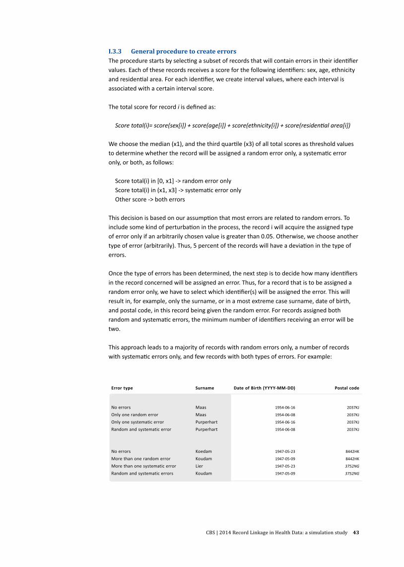
CBS | 2014 Record Linkage in Health Data: a simulation study 43
I.3.3 General procedure to create errorsThe procedure starts by selecting a subset of records that will contain errors in their identifier values. Each of these records receives a score for the following identifiers: sex, age, ethnicity and residential area. For each identifier, we create interval values, where each interval is associated with a certain interval score.
The total score for record i is defined as:
Score total(i)= score(sex[i]) + score(age[i]) + score(ethnicity[i]) + score(residential area[i])
We choose the median (x1), and the third quartile (x3) of all total scores as threshold values to determine whether the record will be assigned a random error only, a systematic error only, or both, as follows:
Score total(i) in [0, x1] -> random error only Score total(i) in (x1, x3] -> systematic error only Other score -> both errors
This decision is based on our assumption that most errors are related to random errors. To include some kind of perturbation in the process, the record i will acquire the assigned type of error only if an arbitrarily chosen value is greater than 0.05. Otherwise, we choose another type of error (arbitrarily). Thus, 5 percent of the records will have a deviation in the type of errors.
Once the type of errors has been determined, the next step is to decide how many identifiers in the record concerned will be assigned an error. Thus, for a record that is to be assigned a random error only, we have to select which identifier(s) will be assigned the error. This will result in, for example, only the surname, or in a most extreme case surname, date of birth, and postal code, in this record being given the random error. For records assigned both random and systematic errors, the minimum number of identifiers receiving an error will be two.
This approach leads to a majority of records with random errors only, a number of records with systematic errors only, and few records with both types of errors. For example:
Error type Surname Date of Birth (YYYY-MM-DD) Postal code
No errors Maas 1954-06-16 2037KJ
Only one random error Maas 1954-06-08 2037KJ
Only one systematic error Purperhart 1954-06-16 2037KJ
Random and systematic error Purperhart 1954-06-08 2037KJ
No errors Koedam 1947-05-23 8442HK
More than one random error Koudam 1947-05-09 8442HK
More than one systematic error Lier 1947-05-23 3752NG
Random and systematic errors Koudam 1947-05-09 3752NG
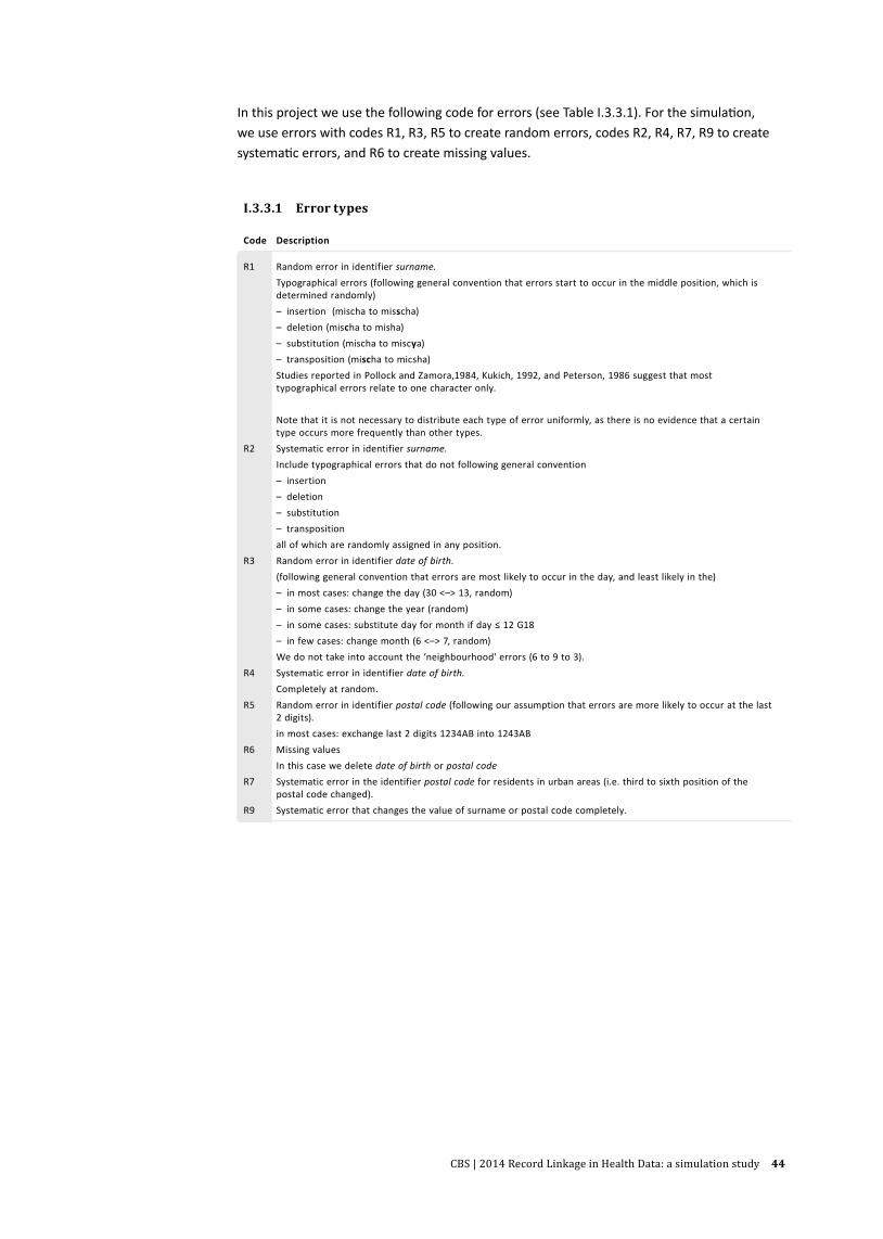
CBS | 2014 Record Linkage in Health Data: a simulation study 44
In this project we use the following code for errors (see Table I.3.3.1). For the simulation, we use errors with codes R1, R3, R5 to create random errors, codes R2, R4, R7, R9 to create systematic errors, and R6 to create missing values.
I.3.3.1 Error types
Code Description
R1 Random error in identifier surname.Typographical errors (following general convention that errors start to occur in the middle position, which is determined randomly)– insertion (mischa to misscha)– deletion (mischa to misha)– substitution (mischa to miscya)– transposition (mischa to micsha)Studies reported in Pollock and Zamora,1984, Kukich, 1992, and Peterson, 1986 suggest that most typographical errors relate to one character only.
Note that it is not necessary to distribute each type of error uniformly, as there is no evidence that a certain type occurs more frequently than other types.
R2 Systematic error in identifier surname.Include typographical errors that do not following general convention– insertion– deletion– substitution– transpositionall of which are randomly assigned in any position.
R3 Random error in identifier date of birth.(following general convention that errors are most likely to occur in the day, and least likely in the)– in most cases: change the day (30 <–> 13, random)– in some cases: change the year (random)– in some cases: substitute day for month if day ≤ 12 G18– in few cases: change month (6 <–> 7, random)We do not take into account the ‘neighbourhood' errors (6 to 9 to 3).
R4 Systematic error in identifier date of birth.Completely at random.
R5 Random error in identifier postal code (following our assumption that errors are more likely to occur at the last 2 digits).in most cases: exchange last 2 digits 1234AB into 1243AB
R6 Missing valuesIn this case we delete date of birth or postal code
R7 Systematic error in the identifier postal code for residents in urban areas (i.e. third to sixth position of the postal code changed).
R9 Systematic error that changes the value of surname or postal code completely.

CBS | 2014 Record Linkage in Health Data: a simulation study 45
II. Appendix II. Blocking results
II.2 Blocking results
Overlap Error
Average number of pairs in
blocking
Average number of
True Positives in blocking
Total number of
True Positives a/b
a b %
S-M 01 01 8,262 159 160 994
S-M 01 02 8,644 156 160 974
S-M 01 03 9,221 154 160 965
S-M 06 01 9,556 948 960 987
S-M 06 02 11,224 930 960 968
S-M 06 03 11,634 911 960 949
S-M 09 01 12,150 1,419 1,440 985
S-M 09 02 12,089 1,397 1,440 970
S-M 09 03 15,185 1,367 1,440 949
S-L 01 01 56,474 158 160 985
S-L 01 02 63,813 157 160 983
S-L 01 03 79,899 151 160 946
S-L 06 01 60,297 944 960 984
S-L 06 02 78,920 923 960 961
S-L 06 03 75,065 910 960 947
S-L 09 01 60,398 1,412 1,440 981
S-L 09 02 68,672 1,392 1,440 966
S-L 09 03 76,899 1,360 1,440 944
M-L 01 01 427,973 1,541 1,600 963
M-L 01 02 472,520 1,506 1,600 941
M-L 01 03 582,814 1,411 1,600 882
M-L 06 01 453,165 9,241 9,600 963
M-L 06 02 511,257 8,861 9,600 923
M-L 06 03 602,118 8,646 9,600 901
M-L 09 01 465,063 13,862 14,400 963
M-L 09 02 595,455 13,418 14,400 932
M-L 09 03 673,702 12,907 14,400 896

CBS | 2014 Record Linkage in Health Data: a simulation study 46
III. Appendix III. Simulation results for other III. linkage keys

CBS | 2014 Record Linkage in Health Data: a simulation study 47
4.3.1.1A The number of total links obtained at each cut-off divided by the number of total links obtained by 4.3.1.1A deterministic. Linkage key: Surname – Date of Birth – Postal code (ndp)
4.3.1.2A The average of precision. Linkage key: Surname – Date of Birth – Postal code (ndp)
data[[xvar]][sel]
data
[[yva
r]][s
el]
S−M
100
120
140
160
180
200
data[[xvar]][sel]
data
[[yva
r]][s
el]
S−L
data[[xvar]][sel]
data
[[yva
r]][s
el]
M−L
0.1
data[[xvar]][sel]
data
[[yva
r]][s
el]
100
120
140
160
180
200
data[[xvar]][sel]
data
[[yva
r]][s
el]
data[[xvar]][sel]
data
[[yva
r]][s
el]
0.6
data[[xvar]][sel]
data
[[yva
r]][s
el]
0 5 10 15 20 25
100
120
140
160
180
200
data[[xvar]][sel]
data
[[yva
r]][s
el]
0 5 10 15 20 25
data[[xvar]][sel]
data
[[yva
r]][s
el]
0 5 10 15 20 25
0.9
Cut−off
Num
ber o
f lin
ks /
num
ber o
f lin
ks d
eter
min
istic
met
hod
(%)
Ove
rlap
Datasets
DeterministicProb.Simple
Prob.JaroProb.Bigram
α= 1.3 α= 1.3 α= 1.3
α= 1.3 α= 1.3 α= 1.3
α= 1.3 α= 1.3 α= 1.3
data[[xvar]][sel]
data
[[yva
r]][s
el]
S−M
20
40
60
80
100
data[[xvar]][sel]
data
[[yva
r]][s
el]
S−L
data[[xvar]][sel]
data
[[yva
r]][s
el]
M−L
0.1
data[[xvar]][sel]
data
[[yva
r]][s
el]
20
40
60
80
100
data[[xvar]][sel]
data
[[yva
r]][s
el]
data[[xvar]][sel]
data
[[yva
r]][s
el]
0.6
data[[xvar]][sel]
data
[[yva
r]][s
el]
0 5 10 15 20 25
20
40
60
80
100
data[[xvar]][sel]
data
[[yva
r]][s
el]
0 5 10 15 20 25
data[[xvar]][sel]
data
[[yva
r]][s
el]
0 5 10 15 20 25
0.9
Cut−off
Prec
isio
n (%
)
Ove
rlap
Datasets
DeterministicProb.Simple
Prob.JaroProb.Bigram
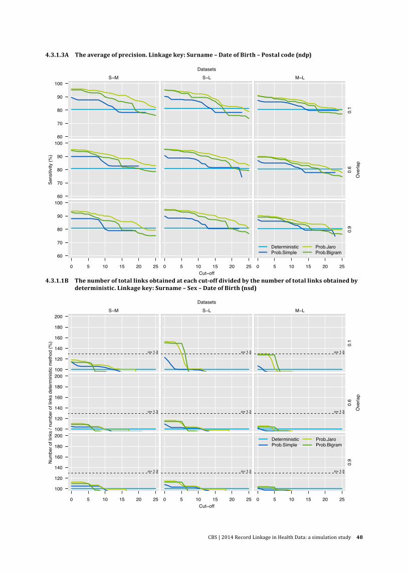
CBS | 2014 Record Linkage in Health Data: a simulation study 48
4.3.1.3A The average of precision. Linkage key: Surname – Date of Birth – Postal code (ndp)
4.3.1.1B The number of total links obtained at each cut-off divided by the number of total links obtained by 4.3.1.1B deterministic. Linkage key: Surname – Sex – Date of Birth (nsd)
data[[xvar]][sel]
data
[[yva
r]][s
el]
S−M
60
70
80
90
100
data[[xvar]][sel]
data
[[yva
r]][s
el]
S−L
data[[xvar]][sel]
data
[[yva
r]][s
el]
M−L
0.1
data[[xvar]][sel]
data
[[yva
r]][s
el]
60
70
80
90
100
data[[xvar]][sel]
data
[[yva
r]][s
el]
data[[xvar]][sel]
data
[[yva
r]][s
el]
0.6
data[[xvar]][sel]
data
[[yva
r]][s
el]
0 5 10 15 20 25
60
70
80
90
100
data[[xvar]][sel]
data
[[yva
r]][s
el]
0 5 10 15 20 25
data[[xvar]][sel]
data
[[yva
r]][s
el]
0 5 10 15 20 25
0.9
Cut−off
Sens
itivi
ty (%
)
Ove
rlap
Datasets
DeterministicProb.Simple
Prob.JaroProb.Bigram
data[[xvar]][sel]
data
[[yva
r]][s
el]
S−M
100
120
140
160
180
200
data[[xvar]][sel]
data
[[yva
r]][s
el]
S−L
data[[xvar]][sel]
data
[[yva
r]][s
el]
M−L
0.1
data[[xvar]][sel]
data
[[yva
r]][s
el]
100
120
140
160
180
200
data[[xvar]][sel]
data
[[yva
r]][s
el]
data[[xvar]][sel]
data
[[yva
r]][s
el]
0.6
data[[xvar]][sel]
data
[[yva
r]][s
el]
0 5 10 15 20 25
100
120
140
160
180
200
data[[xvar]][sel]
data
[[yva
r]][s
el]
0 5 10 15 20 25
data[[xvar]][sel]
data
[[yva
r]][s
el]
0 5 10 15 20 25
0.9
Cut−off
Num
ber o
f lin
ks /
num
ber o
f lin
ks d
eter
min
istic
met
hod
(%)
Ove
rlap
Datasets
DeterministicProb.Simple
Prob.JaroProb.Bigram
α= 1.3 α= 1.3 α= 1.3
α= 1.3 α= 1.3 α= 1.3
α= 1.3 α= 1.3 α= 1.3

CBS | 2014 Record Linkage in Health Data: a simulation study 49
4.3.1.2B The average of precision. Linkage key: Surname – Sex – Date of Birth (nsd)
4.3.1.3B The average of sensitivity. Linkage key: Surname – Sex – Date of Birth (nsd)
data[[xvar]][sel]
data
[[yva
r]][s
el]
S−M
707580859095
100
data[[xvar]][sel]
data
[[yva
r]][s
el]
S−L
data[[xvar]][sel]
data
[[yva
r]][s
el]
M−L
0.1
data[[xvar]][sel]
data
[[yva
r]][s
el]
707580859095
100
data[[xvar]][sel]
data
[[yva
r]][s
el]
data[[xvar]][sel]
data
[[yva
r]][s
el]
0.6
data[[xvar]][sel]
data
[[yva
r]][s
el]
0 5 10 15 20 25
707580859095
100
data[[xvar]][sel]
data
[[yva
r]][s
el]
0 5 10 15 20 25
data[[xvar]][sel]
data
[[yva
r]][s
el]
0 5 10 15 20 25
0.9
Cut−off
Prec
isio
n (%
)
Ove
rlap
Datasets
DeterministicProb.Simple
Prob.JaroProb.Bigram
data[[xvar]][sel]
data
[[yva
r]][s
el]
S−M
60
70
80
90
100
data[[xvar]][sel]
data
[[yva
r]][s
el]
S−L
data[[xvar]][sel]
data
[[yva
r]][s
el]
M−L
0.1
data[[xvar]][sel]
data
[[yva
r]][s
el]
60
70
80
90
100
data[[xvar]][sel]
data
[[yva
r]][s
el]
data[[xvar]][sel]
data
[[yva
r]][s
el]
0.6
data[[xvar]][sel]
data
[[yva
r]][s
el]
0 5 10 15 20 25
60
70
80
90
100
data[[xvar]][sel]
data
[[yva
r]][s
el]
0 5 10 15 20 25
data[[xvar]][sel]
data
[[yva
r]][s
el]
0 5 10 15 20 25
0.9
Cut−off
Sens
itivi
ty (%
)
Ove
rlap
Datasets
DeterministicProb.Simple
Prob.JaroProb.Bigram
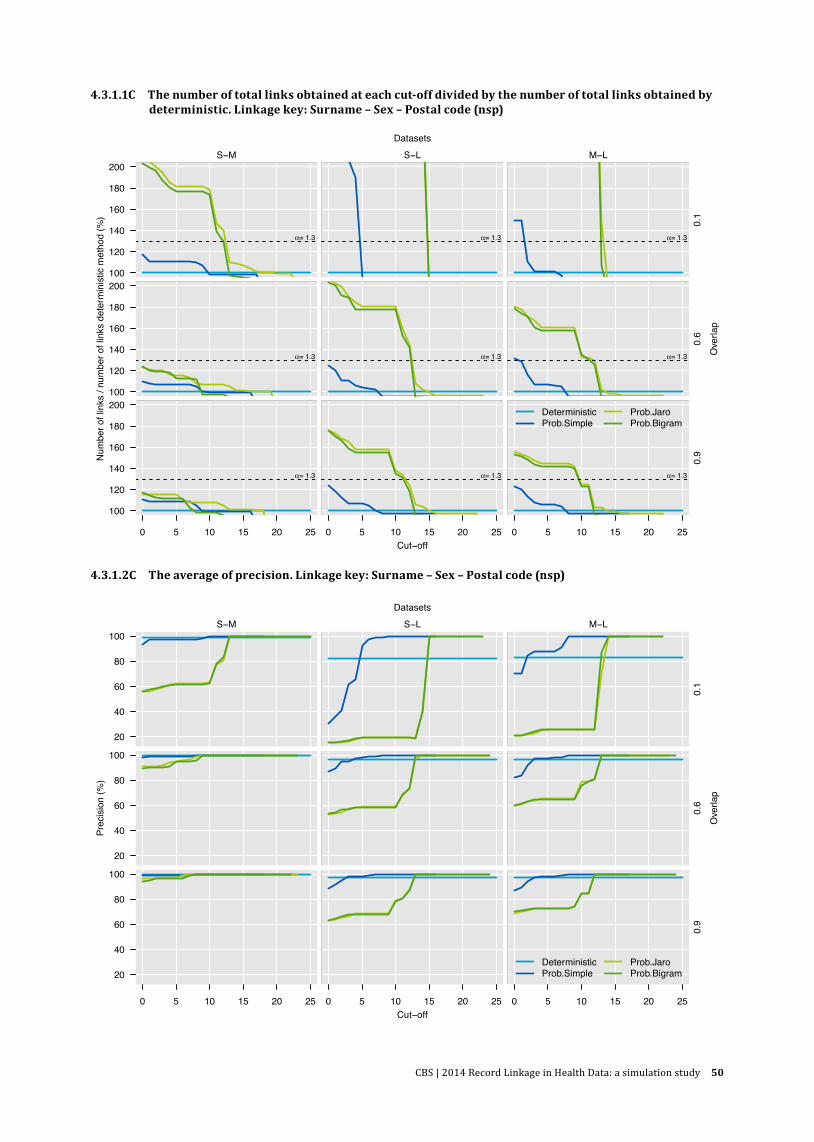
CBS | 2014 Record Linkage in Health Data: a simulation study 50
4.3.1.1C The number of total links obtained at each cut-off divided by the number of total links obtained by 4.3.1.1B deterministic. Linkage key: Surname – Sex – Postal code (nsp)
4.3.1.2C The average of precision. Linkage key: Surname – Sex – Postal code (nsp)
data[[xvar]][sel]
data
[[yva
r]][s
el]
S−M
100
120
140
160
180
200
data[[xvar]][sel]
data
[[yva
r]][s
el]
S−L
data[[xvar]][sel]
data
[[yva
r]][s
el]
M−L
0.1
data[[xvar]][sel]
data
[[yva
r]][s
el]
100
120
140
160
180
200
data[[xvar]][sel]
data
[[yva
r]][s
el]
data[[xvar]][sel]
data
[[yva
r]][s
el]
0.6
data[[xvar]][sel]
data
[[yva
r]][s
el]
0 5 10 15 20 25
100
120
140
160
180
200
data[[xvar]][sel]
data
[[yva
r]][s
el]
0 5 10 15 20 25
data[[xvar]][sel]
data
[[yva
r]][s
el]
0 5 10 15 20 25
0.9
Cut−off
Num
ber o
f lin
ks /
num
ber o
f lin
ks d
eter
min
istic
met
hod
(%)
Ove
rlap
Datasets
DeterministicProb.Simple
Prob.JaroProb.Bigram
α= 1.3 α= 1.3 α= 1.3
α= 1.3 α= 1.3 α= 1.3
α= 1.3 α= 1.3 α= 1.3
data[[xvar]][sel]
data
[[yva
r]][s
el]
S−M
20
40
60
80
100
data[[xvar]][sel]
data
[[yva
r]][s
el]
S−L
data[[xvar]][sel]
data
[[yva
r]][s
el]
M−L
0.1
data[[xvar]][sel]
data
[[yva
r]][s
el]
20
40
60
80
100
data[[xvar]][sel]
data
[[yva
r]][s
el]
data[[xvar]][sel]
data
[[yva
r]][s
el]
0.6
data[[xvar]][sel]
data
[[yva
r]][s
el]
0 5 10 15 20 25
20
40
60
80
100
data[[xvar]][sel]
data
[[yva
r]][s
el]
0 5 10 15 20 25
data[[xvar]][sel]
data
[[yva
r]][s
el]
0 5 10 15 20 25
0.9
Cut−off
Prec
isio
n (%
)
Ove
rlap
Datasets
DeterministicProb.Simple
Prob.JaroProb.Bigram

CBS | 2014 Record Linkage in Health Data: a simulation study 51
data[[xvar]][sel]
data
[[yva
r]][s
el]
S−M
60
70
80
90
100
data[[xvar]][sel]
data
[[yva
r]][s
el]
S−L
data[[xvar]][sel]
data
[[yva
r]][s
el]
M−L
0.1
data[[xvar]][sel]
data
[[yva
r]][s
el]
60
70
80
90
100
data[[xvar]][sel]
data
[[yva
r]][s
el]
data[[xvar]][sel]
data
[[yva
r]][s
el]
0.6
data[[xvar]][sel]
data
[[yva
r]][s
el]
0 5 10 15 20 25
60
70
80
90
100
data[[xvar]][sel]
data
[[yva
r]][s
el]
0 5 10 15 20 25
data[[xvar]][sel]
data
[[yva
r]][s
el]
0 5 10 15 20 25
0.9
Cut−off
Sens
itivi
ty (%
)
Ove
rlap
Datasets
DeterministicProb.Simple
Prob.JaroProb.Bigram
4.3.1.3C The average of sensitivity. Linkage key: Surname – Sex – Postal code (nsp)
4.3.1.1D The number of total links obtained at each cut-off divided by the number of total links obtained by 4.3.1.1B deterministic. Linkage key: Sex– Date of Birth – Postal code (sdp)
data[[xvar]][sel]
data
[[yva
r]][s
el]
S−M
100
120
140
160
180
200
data[[xvar]][sel]
data
[[yva
r]][s
el]
S−L
data[[xvar]][sel]
data
[[yva
r]][s
el]
M−L
0.1
data[[xvar]][sel]
data
[[yva
r]][s
el]
100
120
140
160
180
200
data[[xvar]][sel]
data
[[yva
r]][s
el]
data[[xvar]][sel]
data
[[yva
r]][s
el]
0.6
data[[xvar]][sel]
data
[[yva
r]][s
el]
0 5 10 15
100
120
140
160
180
200
data[[xvar]][sel]
data
[[yva
r]][s
el]
0 5 10 15
data[[xvar]][sel]
data
[[yva
r]][s
el]
0 5 10 15
0.9
Cut−off
Num
ber o
f lin
ks /
num
ber o
f lin
ks d
eter
min
istic
met
hod
(%)
Ove
rlap
Datasets
DeterministicProb.Simple
Prob.JaroProb.Bigram
α= 1.3 α= 1.3 α= 1.3
α= 1.3 α= 1.3 α= 1.3
α= 1.3 α= 1.3 α= 1.3

CBS | 2014 Record Linkage in Health Data: a simulation study 52
4.3.1.2D The average of precision. Linkage key: Sex– Date of Birth – Postal code (sdp)
4.3.1.3D The average of sensitivity. Linkage key: Sex– Date of Birth – Postal code (sdp)
data[[xvar]][sel]
data
[[yva
r]][s
el]
S−M
40
60
80
100
data[[xvar]][sel]
data
[[yva
r]][s
el]
S−L
data[[xvar]][sel]
data
[[yva
r]][s
el]
M−L
0.1
data[[xvar]][sel]
data
[[yva
r]][s
el]
40
60
80
100
data[[xvar]][sel]
data
[[yva
r]][s
el]
data[[xvar]][sel]
data
[[yva
r]][s
el]
0.6
data[[xvar]][sel]
data
[[yva
r]][s
el]
0 5 10 15
40
60
80
100
data[[xvar]][sel]
data
[[yva
r]][s
el]
0 5 10 15
data[[xvar]][sel]
data
[[yva
r]][s
el]
0 5 10 15
0.9
Cut−off
Prec
isio
n (%
)
Ove
rlap
Datasets
DeterministicProb.Simple
Prob.JaroProb.Bigram
data[[xvar]][sel]
data
[[yva
r]][s
el]
S−M
60
70
80
90
100
data[[xvar]][sel]
data
[[yva
r]][s
el]
S−L
data[[xvar]][sel]
data
[[yva
r]][s
el]
M−L
0.1
data[[xvar]][sel]
data
[[yva
r]][s
el]
60
70
80
90
100
data[[xvar]][sel]
data
[[yva
r]][s
el]
data[[xvar]][sel]
data
[[yva
r]][s
el]
0.6
data[[xvar]][sel]
data
[[yva
r]][s
el]
0 5 10 15
60
70
80
90
100
data[[xvar]][sel]
data
[[yva
r]][s
el]
0 5 10 15
data[[xvar]][sel]
data
[[yva
r]][s
el]
0 5 10 15
0.9
Cut−off
Sens
itivi
ty (%
)
Ove
rlap
Datasets
DeterministicProb.Simple
Prob.JaroProb.Bigram
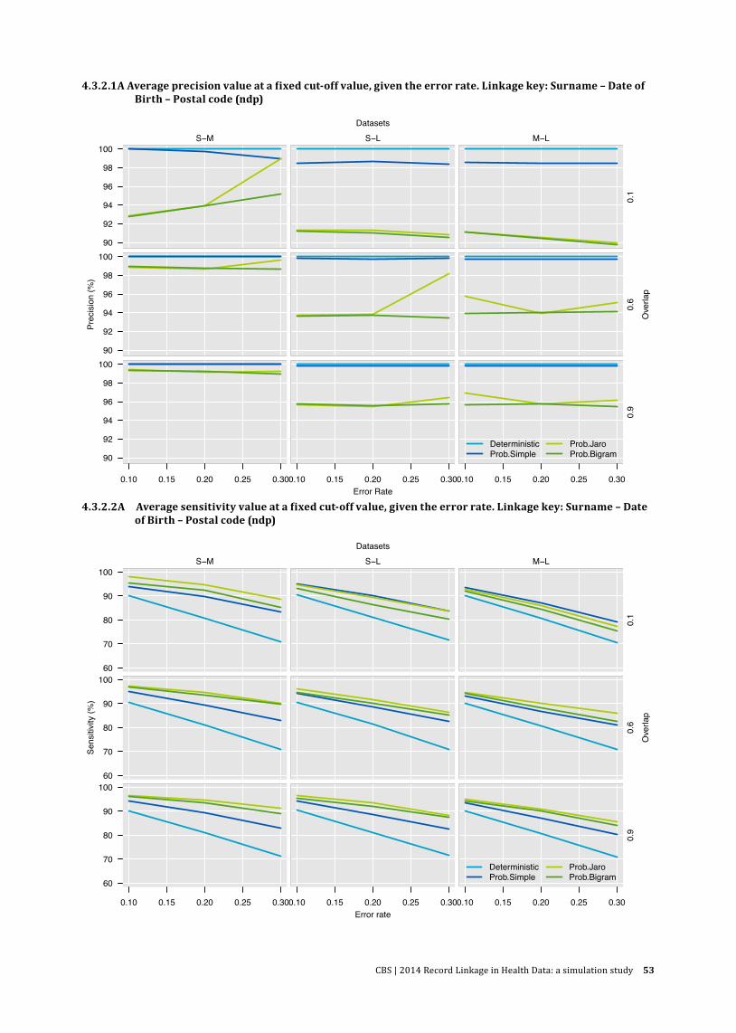
CBS | 2014 Record Linkage in Health Data: a simulation study 53
4.3.2.1A Average precision value at a fixed cut-off value, given the error rate. Linkage key: Surname – Date of 4.3.1.1B Birth – Postal code (ndp)
4.3.2.2A Average sensitivity value at a fixed cut-off value, given the error rate. Linkage key: Surname – Date 4.3.1.1B of Birth – Postal code (ndp)
data[[xvar]][sel]
data
[[yva
r]][s
el]
S−M
90
92
94
96
98
100
data[[xvar]][sel]
data
[[yva
r]][s
el]
S−L
data[[xvar]][sel]
data
[[yva
r]][s
el]
M−L
0.1
data[[xvar]][sel]
data
[[yva
r]][s
el]
90
92
94
96
98
100
data[[xvar]][sel]
data
[[yva
r]][s
el]
data[[xvar]][sel]
data
[[yva
r]][s
el]
0.6
data[[xvar]][sel]
data
[[yva
r]][s
el]
0.10 0.15 0.20 0.25 0.30
90
92
94
96
98
100
data[[xvar]][sel]
data
[[yva
r]][s
el]
0.10 0.15 0.20 0.25 0.30
data[[xvar]][sel]
data
[[yva
r]][s
el]
0.10 0.15 0.20 0.25 0.30
0.9
Error Rate
Prec
isio
n (%
)
Ove
rlap
Datasets
DeterministicProb.Simple
Prob.JaroProb.Bigram
data[[xvar]][sel]
data
[[yva
r]][s
el]
S−M
60
70
80
90
100
data[[xvar]][sel]
data
[[yva
r]][s
el]
S−L
data[[xvar]][sel]
data
[[yva
r]][s
el]
M−L
0.1
data[[xvar]][sel]
data
[[yva
r]][s
el]
60
70
80
90
100
data[[xvar]][sel]
data
[[yva
r]][s
el]
data[[xvar]][sel]
data
[[yva
r]][s
el]
0.6
data[[xvar]][sel]
data
[[yva
r]][s
el]
0.10 0.15 0.20 0.25 0.30
60
70
80
90
100
data[[xvar]][sel]
data
[[yva
r]][s
el]
0.10 0.15 0.20 0.25 0.30
data[[xvar]][sel]
data
[[yva
r]][s
el]
0.10 0.15 0.20 0.25 0.30
0.9
Error rate
Sens
itivi
ty (%
)
Ove
rlap
Datasets
DeterministicProb.Simple
Prob.JaroProb.Bigram
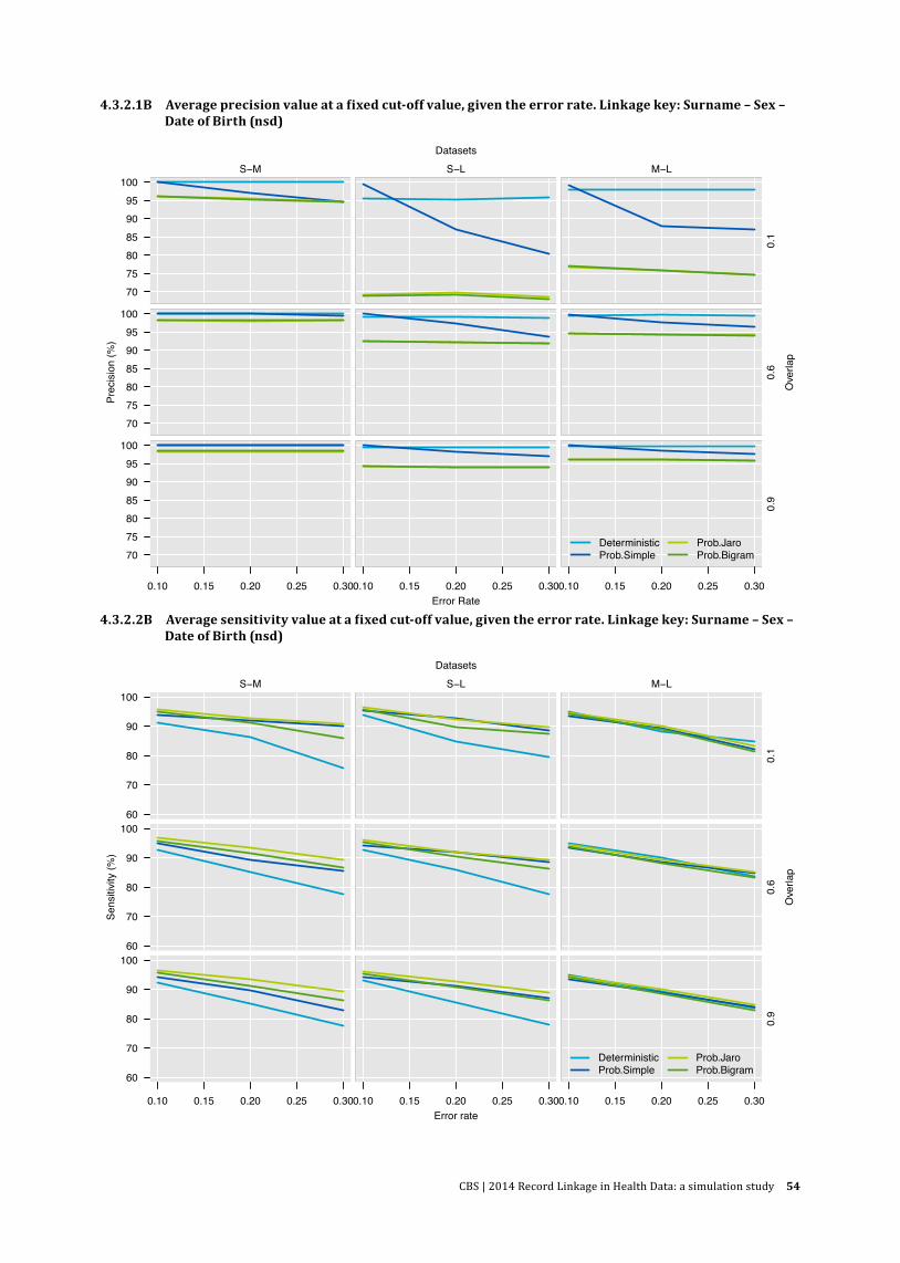
CBS | 2014 Record Linkage in Health Data: a simulation study 54
4.3.2.1B Average precision value at a fixed cut-off value, given the error rate. Linkage key: Surname – Sex – 4.3.1.1B Date of Birth (nsd)
4.3.2.2B Average sensitivity value at a fixed cut-off value, given the error rate. Linkage key: Surname – Sex – 4.3.1.1B Date of Birth (nsd)
data[[xvar]][sel]
data
[[yva
r]][s
el]
S−M
707580859095
100
data[[xvar]][sel]
data
[[yva
r]][s
el]
S−L
data[[xvar]][sel]
data
[[yva
r]][s
el]
M−L
0.1
data[[xvar]][sel]
data
[[yva
r]][s
el]
707580859095
100
data[[xvar]][sel]
data
[[yva
r]][s
el]
data[[xvar]][sel]
data
[[yva
r]][s
el]
0.6
data[[xvar]][sel]
data
[[yva
r]][s
el]
0.10 0.15 0.20 0.25 0.30
707580859095
100
data[[xvar]][sel]
data
[[yva
r]][s
el]
0.10 0.15 0.20 0.25 0.30
data[[xvar]][sel]
data
[[yva
r]][s
el]
0.10 0.15 0.20 0.25 0.30
0.9
Error Rate
Prec
isio
n (%
)
Ove
rlap
Datasets
DeterministicProb.Simple
Prob.JaroProb.Bigram
data[[xvar]][sel]
data
[[yva
r]][s
el]
S−M
60
70
80
90
100
data[[xvar]][sel]
data
[[yva
r]][s
el]
S−L
data[[xvar]][sel]
data
[[yva
r]][s
el]
M−L
0.1
data[[xvar]][sel]
data
[[yva
r]][s
el]
60
70
80
90
100
data[[xvar]][sel]
data
[[yva
r]][s
el]
data[[xvar]][sel]
data
[[yva
r]][s
el]
0.6
data[[xvar]][sel]
data
[[yva
r]][s
el]
0.10 0.15 0.20 0.25 0.30
60
70
80
90
100
data[[xvar]][sel]
data
[[yva
r]][s
el]
0.10 0.15 0.20 0.25 0.30
data[[xvar]][sel]
data
[[yva
r]][s
el]
0.10 0.15 0.20 0.25 0.30
0.9
Error rate
Sens
itivi
ty (%
)
Ove
rlap
Datasets
DeterministicProb.Simple
Prob.JaroProb.Bigram
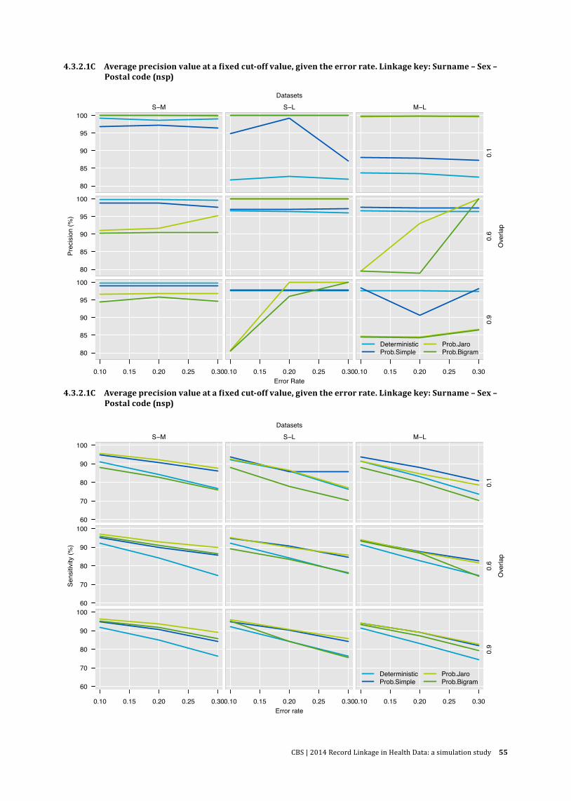
CBS | 2014 Record Linkage in Health Data: a simulation study 55
4.3.2.1C Average precision value at a fixed cut-off value, given the error rate. Linkage key: Surname – Sex – 4.3.1.1B Postal code (nsp)
4.3.2.1C Average precision value at a fixed cut-off value, given the error rate. Linkage key: Surname – Sex – 4.3.1.1B Postal code (nsp)
data[[xvar]][sel]
data
[[yva
r]][s
el]
S−M
80
85
90
95
100
data[[xvar]][sel]
data
[[yva
r]][s
el]
S−L
data[[xvar]][sel]
data
[[yva
r]][s
el]
M−L
0.1
data[[xvar]][sel]
data
[[yva
r]][s
el]
80
85
90
95
100
data[[xvar]][sel]
data
[[yva
r]][s
el]
data[[xvar]][sel]
data
[[yva
r]][s
el]
0.6
data[[xvar]][sel]
data
[[yva
r]][s
el]
0.10 0.15 0.20 0.25 0.30
80
85
90
95
100
data[[xvar]][sel]
data
[[yva
r]][s
el]
0.10 0.15 0.20 0.25 0.30
data[[xvar]][sel]
data
[[yva
r]][s
el]
0.10 0.15 0.20 0.25 0.30
0.9
Error Rate
Prec
isio
n (%
)
Ove
rlap
Datasets
DeterministicProb.Simple
Prob.JaroProb.Bigram
data[[xvar]][sel]
data
[[yva
r]][s
el]
S−M
60
70
80
90
100
data[[xvar]][sel]
data
[[yva
r]][s
el]
S−L
data[[xvar]][sel]
data
[[yva
r]][s
el]
M−L
0.1
data[[xvar]][sel]
data
[[yva
r]][s
el]
60
70
80
90
100
data[[xvar]][sel]
data
[[yva
r]][s
el]
data[[xvar]][sel]
data
[[yva
r]][s
el]
0.6
data[[xvar]][sel]
data
[[yva
r]][s
el]
0.10 0.15 0.20 0.25 0.30
60
70
80
90
100
data[[xvar]][sel]
data
[[yva
r]][s
el]
0.10 0.15 0.20 0.25 0.30
data[[xvar]][sel]
data
[[yva
r]][s
el]
0.10 0.15 0.20 0.25 0.30
0.9
Error rate
Sens
itivi
ty (%
)
Ove
rlap
Datasets
DeterministicProb.Simple
Prob.JaroProb.Bigram
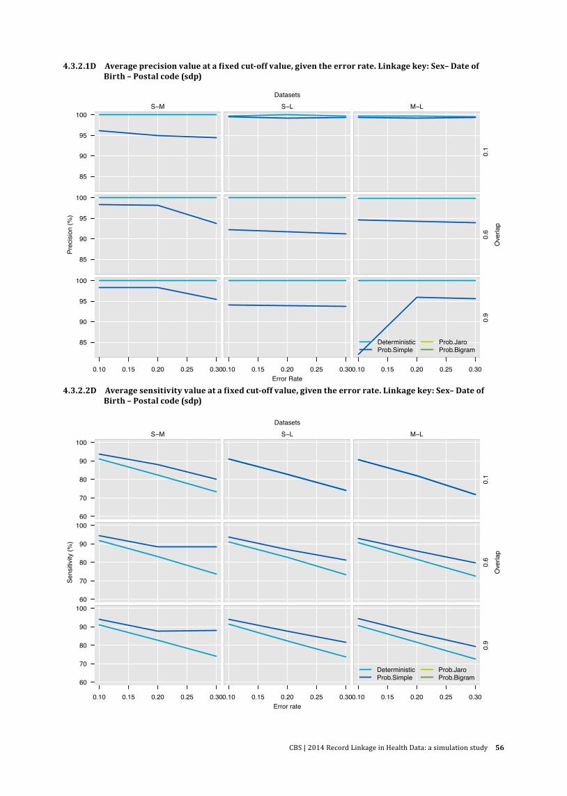
CBS | 2014 Record Linkage in Health Data: a simulation study 56
data[[xvar]][sel]
data
[[yva
r]][s
el]
S−M
85
90
95
100
data[[xvar]][sel]
data
[[yva
r]][s
el]
S−L
data[[xvar]][sel]
data
[[yva
r]][s
el]
M−L
0.1
data[[xvar]][sel]
data
[[yva
r]][s
el]
85
90
95
100
data[[xvar]][sel]
data
[[yva
r]][s
el]
data[[xvar]][sel]
data
[[yva
r]][s
el]
0.6
data[[xvar]][sel]
data
[[yva
r]][s
el]
0.10 0.15 0.20 0.25 0.30
85
90
95
100
data[[xvar]][sel]
data
[[yva
r]][s
el]
0.10 0.15 0.20 0.25 0.30
data[[xvar]][sel]
data
[[yva
r]][s
el]
0.10 0.15 0.20 0.25 0.30
0.9
Error Rate
Prec
isio
n (%
)
Ove
rlap
Datasets
DeterministicProb.Simple
Prob.JaroProb.Bigram
4.3.2.1D Average precision value at a fixed cut-off value, given the error rate. Linkage key: Sex– Date of 4.3.1.1B Birth – Postal code (sdp)
4.3.2.2D Average sensitivity value at a fixed cut-off value, given the error rate. Linkage key: Sex– Date of 4.3.1.1B Birth – Postal code (sdp)
data[[xvar]][sel]
data
[[yva
r]][s
el]
S−M
60
70
80
90
100
data[[xvar]][sel]
data
[[yva
r]][s
el]
S−L
data[[xvar]][sel]
data
[[yva
r]][s
el]
M−L
0.1
data[[xvar]][sel]
data
[[yva
r]][s
el]
60
70
80
90
100
data[[xvar]][sel]
data
[[yva
r]][s
el]
data[[xvar]][sel]
data
[[yva
r]][s
el]
0.6
data[[xvar]][sel]
data
[[yva
r]][s
el]
0.10 0.15 0.20 0.25 0.30
60
70
80
90
100
data[[xvar]][sel]
data
[[yva
r]][s
el]
0.10 0.15 0.20 0.25 0.30
data[[xvar]][sel]
data
[[yva
r]][s
el]
0.10 0.15 0.20 0.25 0.30
0.9
Error rate
Sens
itivi
ty (%
)
Ove
rlap
Datasets
DeterministicProb.Simple
Prob.JaroProb.Bigram
CBS | 2014 Record Linkage in Health Data: a simulation study 57
References
Adams MM, Wilson HG, Casto DL, Berg CJ, McDermott JM, Gaudino JA, McCarthy BJ. 1997. Constructing reproductive histories by linking vital records. American Journal of Epidemiology 145:339–348.
Arts K, Bakker BFM, van Lith E. 2000. Linking administrative registers and household surveys. Netherlands Official Statistics, 15, 16–22. Netherlands Official Statistics.
Bakker BFM. 2002. Statistics Netherlands’ approach to social statistics: the social statistical dataset. OECD Statistics Newsletter 2002:4–6.
Bakker BFM, Daas P. 2012. Some methodological issues of register based research. Statistica Neerlandica 66:2–7.
Bauman Jr. GJ. 2006. Computations of weights for probabilistic record linkage using the EM algorithm. Brigham Young University.
Bergman L, Beelen MLR, Gallee MPW, Hollema H, Benraadt J, van Leeuwen FE. 2000. Risk and prognosis of endometrial cancer after tamoxifen for breast cancer. Lancet 356:881–887.
Blakely T, Woodward A, Salmond C. 2000. Anonymous linkage of New Zealand mortality and Census data. Australian and New Zealand Journal of Public Health 24:92–95.
Bozkurt O, de Boer A, Grobbee DE, de Leeuw PW, Kroon AA, Schiffers P, Klungel OH. 2009. Variation in Renin-Angiotensin System and Salt-Sensitivity Genes and the Risk of Diabetes Mellitus Associated With the Use of Thiazide Diuretics. American Journal of Hypertension 22:545–551.
Christen P, Pudjijono A. Accurate synthetic generation of realistic personal information. 2009; Bangkok, Thailand. 507–514.
Churches T, Christen P. 2004a. Blind data linkage using n-gram similarity comparisons. 126.
Churches T, Christen P. 2004b. Some methods for blindfolded record linkage. Bmc Medical Informatics and Decision Making 4:9.
de Bruin A, de Bruin EI, Gast A, Kardaun JWPF, van Sijl M, Verweij GJG. 2003. Koppeling van LMR- en GBA-gegevens: methode, resultaten en kwaliteitsonderzoek. Statistics Netherlands.
Dean JM, Vernon DD, Cook L, Nechodom P, Reading J, Suruda A. 2001. Probabilistic linkage of computerized ambulance and inpatient hospital discharge records: A potential tool for evaluation of emergency medical services. Annals of Emergency Medicine 37:616–626.
Dempster AP, Laird NM, Rubin DB. 1977. Maximum Likelihood from Incomplete Data Via Em Algorithm. Journal of the Royal Statistical Society Series B-Methodological 39:1–38.

CBS | 2014 Record Linkage in Health Data: a simulation study 58
Durham E, Xue Y, Kantarcioglu M, Malin B. 2012. Quantifying the correctness, computational complexity, and security of privacy-preserving string comparators for record linkage. Information Fusion 13:245–259.
DuVall SL, Kerber RA, Thomas A. 2010. Extending the Fellegi-Sunter probabilistic record linkage method for approximate field comparators. Journal of Biomedical Informatics 43:24–30.
Elfeky MG, Verykios VS, Elmagarmid AK. TAILOR: A Record Linkage Toolbox. 2002.
Eussen SR, de Jong N, Rompelberg CJ, Garssen J, Verschuren W, Klungel OH. 2010. Effects of the use of phytosterol/-stanol-enriched margarines on adherence to statin therapy. Pharmacoepidemiology and Drug Safety 19:1225–1232.
Fellegi IP, Sunter AB. 1969. A Theory for Record Linkage. Journal of the American Statistical Association 64:1183–1210.
Fienberg SE, Manrique-Vallier D. 2009. Integrated methodology for multiple systems estimation and record linkage using a missing data formulation. Asta-Advances in Statistical Analysis 93:49–60.
Florentinus SR, Souverein PC, Griens FAMG, Groenewegen PP, Leufkens HGM, Heerdink ER. 2006. Linking community pharmacy dispensing data to prescribing data of general practitioners. Bmc Medical Informatics and Decision Making 6.
Fournel I, Schwarzinger M, Binquet C, Benzenine E, Hill C, Quantin C. 2009. Contribution of record linkage to vital status determination in cancer patients. Studies in health technology and informatics 150:91–95.
Giersiepen K, Bachteler T, Gramlich T, Reiher J, Schubert B, Novopashenny I, Schnell R. 2010. Performance of record linkage for cancer registry data linked with mammography screening data. Bundesgesundheitsblatt-Gesundheitsforschung-Gesundheitsschutz 53:740–747.
Gomatam S, Carter R, Ariet M, Mitchell G. 2002. An empirical comparison of record linkage procedures. Statistics in Medicine 21:1485–1496.
Gorelick MH, Knight S, Alessandrini EA, Stanley RM, Chamberlain JM, Kuppermann N, Alpern ER. 2007. Lack of agreement in pediatric emergency department discharge diagnoses from clinical and administrative data sources. Academic Emergency Medicine 14:646–652.
Gu LF, Li JY, He HX, Williams G, Hawkins S, Kelman C. 2003. Association rule discovery with unbalanced class distributions. Ai 2003: Advances in Artificial Intelligence 2903:221–232.
Hammill BG, Hernandez AF, Peterson ED, Fonarow GC, Schulman KA, Curtis LH. 2009. Linking inpatient clinical registry data to Medicare claims data using indirect identifiers. American Heart Journal 157:995–1000.
Herings RMC. 1993. PHARMO: A record linkage system for postmarketing surveillance of prescription drugs in The Netherlands. Utrecht University.

CBS | 2014 Record Linkage in Health Data: a simulation study 59
Hernandez MA, Stolfo SJ. 1998. Real-world data is dirty: data cleansing and the merge/purge problem. Journal of Data Mining and Knowledge Discovery 2; 2–87.
Hernandez MA, Stolfo SJ. The Merge/Purge Problem for Large Databases. 1995; 127–138.
Hockley C, Quigley MA, Hughes G, Calderwood L, Joshi H, Davidson LL. 2008. Linking Millennium Cohort data to birth registration and hospital episode records. Paediatric and Perinatal Epidemiology 22:99–109.
Hser YI, Evans E. 2008. Cross-system data linkage for treatment outcome evaluation: Lessons learned from the California Treatment Outcome Project. Evaluation and Program Planning 31:125–135.
Jaro MA. 1989. Advances in Record-Linkage Methodology As Applied to Matching the 1985 Census of Tampa, Florida. Journal of the American Statistical Association 84:414–420.
Jaro MA. 1995. Probabilistic Linkage of Large Public-Health Data Files. Statistics in Medicine 14:491–498.
Karakasidis A, Verykios V. Privacy Preserving Record Linkage Using Phonetic Codes. 2009; 101–106.
Karmel R, Anderson P, Gibson D, Peut A, Duckett S, Wells Y. 2010. Empirical aspects of record linkage across multiple data sets using statistical linkage keys: the experience of the PIAC cohort study. Bmc Health Services Research 10; 4.
Kirsch A, Mitzenmacher M. 2008. Less hashing, same performance: Building a better Bloom filter. Random Structures & Algorithms 33:187–218.
L.Gu, R.Baxter, D.Vickers, C.Rainsford. 2003. Record linkage: Current practice and future directions. Canberra: CSIRO Mathematical and Information Science.
Lain SJ, Algert CS, Tasevski V, Morris JM, Roberts CL. 2009. Record linkage to obtain birth outcomes for the evaluation of screening biomarkers in pregnancy: a feasibility study. Bmc Medical Research Methodology 9; 8.
Levenhstein VI. 1966. Binary codes capable of correcting deletions, insertions and reversals. Soviet Physics Doklady 10:707–710.
Lyons RA, Jones KH, John G, Brooks CJ, Verplancke JP, Ford DV, Brown G, Leake K. 2009. The SAIL databank: linking multiple health and social care datasets. Bmc Medical Informatics and Decision Making 9; 3.
Marquez Cid M, Chirlaque M, Navarro C. 2008. DataLink Record Linkage Software Applied to the Cancer Registry of Murcia, Spain. Methods of Information in Medicine 47:448–453.
McCallum A, Nigam K, Ungar L. Learning to Match and Cluster Large High Dimensional Data Sets for Data Integration. 2000; 169–170.
CBS | 2014 Record Linkage in Health Data: a simulation study 60
McCoy SI, Jones B, Leone PA, Napravnik S, Quinlivan EB, Eron JJ, Miller WC. 2010. Variability of the Date of HIV Diagnosis: A Comparison of Self-Report, Medical Record, and HIV/AIDS Surveillance Data. Annals of Epidemiology 20:734–742.
Meray N, Reitsma JB, Ravelli AC, Bonsel GJ. 2007. Probabilistic record linkage is a valid and transparent tool to combine databases without a patient identification number. Journal of Clinical Epidemiology 60:883–891.
Newcombe HB. 1994. Cohorts and Privacy. Cancer Causes & Control 5:287–291.
Newcombe HB, Fair ME, Lalonde P. 1992. The Use of Names for Linking Personal Records. Journal of the American Statistical Association 87:1193–1204.
Newcombe HB, Kennedy JM, Axford SJ, James AP. 1959. Automatic Linkage of Vital Records. Science 130:954–959.
Newgard C, Malveau S, Staudenmayer K, Wang N, Hsia RY, Mann N, Holmes JF, Kuppermann N, Haukoos JS, Bulger EM and others. 2012. Evaluating the Use of Existing Data Sources, Probabilistic Linkage, and Multiple Imputation to Build Population-based Injury Databases Across Phases of Trauma Care. Academic Emergency Medicine 19:469–480.
Oberaigner W. 2007. Errors in survival rates caused by routinely used deterministic record linkage methods. Methods of Information in Medicine 46:420–424.
Pacheco AG, Saraceni V, Tuboi SH, Moulton LH, Chaisson RE, Cavalcante SC, Durovni B, Faulhaber JC, Golub JE, King B and others. 2008. Validation of a Hierarchical Deterministic Record-Linkage Algorithm Using Data From 2 Different Cohorts of Human Immunodeficiency Virus-Infected Persons and Mortality Databases in Brazil. American Journal of Epidemiology 168:1326–1332.
Pasquali SK, Jacobs JP, Shook GJ, O’Brien SM, Hall M, Jacobs ML, Welke KF, Gaynor J, Peterson ED, Shah SS and others. 2010. Linking clinical registry data with administrative data using indirect identifiers: Implementation and validation in the congenital heart surgery population. American Heart Journal 160:1099–1104.
Porter EH, Winkler WE. 1997. Approximate string comparison and its effect on an advanced record linkage system. SRD research report .
Pukkala E. 2008. Biobanks and registers in Epidemiological Research on Cancer In: Dilmer J, editor. Methods in Biobanking. Berlin: Springer Verlag. p 127–164.
Quantin C, Binquet C, Allaert FA, Cornet B, Pattisina R, Leteuff G, Ferdynus C, Gouyon JB. 2005. Decision analysis for the assessment of a record linkage procedure – Application to a perinatal network. Methods of Information in Medicine 44:72–79.
Reitsma JB. 1999. Registers in cardiovascular epidemiology. UVA University.
Roos LL, Walld R, Wajda A, Bond R, Hartford K. 1996. Record linkage strategies, outpatient procedures, and administrative data. Medical Care 34:570–582.

CBS | 2014 Record Linkage in Health Data: a simulation study 61
Schelleman H, Stricker BHC, Verschuren WMM, de Boer A, Kroon AA, de Leeuw PW, Kromhout D, Klungel OH. 2006. Interactions between five candidate genes and antihypertensive drug therapy on blood pressure. Pharmacogenomics Journal 6:22–26.
Schnell R, Bachteler T, Reiher J. 2009. Privacy-preserving record linkage using Bloom filters. Bmc Medical Informatics and Decision Making 9.
Silveira DP, Artmann E. 2009. Accuracy of probabilistic record linkage applied to health databases: systematic review. Revista de saude publica 43:875–882.
Theis MK, Reid RJ, Chaudhari M, Newton KM, Spangler L, Grossman DC, Inge RE. 2010. Case Study of Linking Dental and Medical Healthcare Records. American Journal of Managed Care 16:E51–E56.
Trepetin S. 2008. Privacy-preserving string comparisons in record linkage system: a review. Information Security Journal: A global perspective 17:253–266.
Tromp M, Reitsma JB, Ravelli ACJ, Meray N, Bonsel GJ. 2006. Record linkage: making the most out of errors in linking variables. AMIA Annual Symposium proceedings / AMIA Symposium AMIA Symposium 779–783.
Tromp M, van Eijsden M, Ravelli A, Bonsel G. 2009. Anonymous non-response analysis in the ABCD cohort study enabled by probabilistic record linkage. Paediatric and Perinatal Epidemiology 23:264–272.
Tromp M, Ravelli AC, Bonsel GJ, Hasman A, Reitsma JB. 2011. Results from simulated data sets: probabilistic record linkage outperforms deterministic record linkage. Journal of Clinical Epidemiology 64:565–572.
Turchin A, Shubina M, Murphy SN. 2010. I am Not Dead Yet: Identification of False-Positive Matches to Death Master File. AMIA Annual Symposium proceedings / AMIA Symposium AMIA Symposium 2010:807–811.
Van den Brandt PA, Schouten LJ, Goldbohm RA, Dorant E, Hunen PMH. 1990. Development of A Record Linkage Protocol for Use in the Dutch Cancer Registry for Epidemiologic Research. International Journal of Epidemiology 19:553–558.
van der Laan DJ. 2013. Optimal threshold when training data are available. Personal Communication.
van Herk-Sukel MP, Lemmens VE, van de Poll-Franse L, Herings RM, Coebergh JW. 2012a. Record linkage for pharmacoepidemiological studies in cancer patients. Pharmacoepidemiology and Drug Safety 21:94–103.
Verykios VS, Moustakides GV, Elfeky MG. 2002. A Bayesian Decision Model for Cost Optimal Record Matching. The VLDB Journal 12:28–40.
Victor TW, Mera RM. 2001. Record linkage of health care insurance claims. Journal of the American Medical Informatics Association 8:281–288.

CBS | 2014 Record Linkage in Health Data: a simulation study 62
Vink J, Sadrzadeh S, Lambalk C, Boomsma D, I. 2006. Heritability of polycystic ovary syndrome in a Dutch twin-family study. Journal of Clinical Endocrinology & Metabolism 91:2100–2104.
Wallgren A, Wallgren B. 2007. Register-based Statistics: Administrative Data for Statistical Purposes. New York: Wiley.
Weber SC, Lowe HJ, Das A, Ferris TA. 2012. A simple heuristic for blindfolded record linkage. Journal of the American Medical Informatics Association, 19, e157–e161.
Winkler WE. 2006. Overview of record linkage and current research directions.
Yancey W. Improving EM Algorithm Estimates for Record Linkage Parameters. 2002.
Zhu VJ, Overhage MJ, Egg J, Downs SM, Grannis SJ. 2009. An Empiric Modification to the Probabilistic Record Linkage Algorithm Using Frequency-Based Weight Scaling. Journal of the American Medical Informatics Association 16:738–745.
Glossary
Biobank A collection of biomedical samples along with medical, genetic, genealogic, and other data about the donors (subjects), for research purposes. (Brandsma, M., Meerjarenplan BBMRI-NL Fase 1 (2009–2012), 2010, p 25).
Unlike registers and cohorts, a biobank usually contains objects without complete personal data.
CohortAny designated group of persons followed or traced over a period of time to examine health or mortality experience. Cohorts can be subsets of registers and databases.
Example: The DCIS (Ductal Carcinoma in Situ) cohort is a part of the National Cancer Register in the Netherlands: all women diagnosed with DCIS as the first tumour between 1989–2004.
DatabaseAn electronic data collection that is systematically organized and has a logical structure and relationship. Data from registers, cohorts, or biobanks can be stored in a database.
RegisterA collection of data about samples or subjects designed to fulfil a specific purpose.A register is a database whose records meet all the criteria defined by the purpose of the register.
Example: the National Cancer Register in the Netherlands (NKR) collects data on patients who have developed cancer, while Dutch Municipal Administration (GBA) registers the Dutch population.

CBS | 2014 Record Linkage in Health Data: a simulation study 63
Authors
Adelaide Ariel is a methodologist within the Biolink NL project at GGZ inGeest in Amsterdam. She selected the linkage methods for evaluation, designed and performed the simulations, and drafted the paper.
Bart F.M. Bakker is the manager of the Methodology team at Statistics Netherlands in The Hague and professor at the Faculty of Social Sciences of VU University Amsterdam. He was overall responsible for the outcomes of the record linkage simulation.
Mark C. H. de Groot is a researcher at the department of Pharmacoepidemiology and Clinical Pharmacology of the Utrecht University. He has been involved in multiple health data linkages in The Netherlands.
Gerard van Grootheest works as a data manager and biobank coordinator at the research department of GGZ inGeest and the department of Psychiatry of the VU University medical center in Amsterdam, and is part-time project manager of Biolink NL.
Dingeman Jan van der Laan is a methodologist at the Methodology team of Statistics Netherlands in The Hague. He specialises in probabilistic record linkage of general population registers.
Johannes H. Smit is managing director of research of the Department of Psychiatry, director of the Cohort Research knowledge centre at the VU University medical center in Amsterdam, and professor at the chair ‘Methodology of longitudinal psychiatric research’. He is one of the principal investigators of the Biolink NL project.
Bep C.M. Verkerk has worked as a data manager and quality coordinator at various research institutes and health registries. She co-developed the simulation sets and carried out the various linkage algorithms for the current paper.
The current paper was written as part of Biolink NL, one of the so-called rainbow projects funded by the Dutch Biobanking and Biomolecular Resources Research Infrastructure (BBMRI-NL).

CBS | 2014 Record Linkage in Health Data: a simulation study 64
PublisherStatistics NetherlandsHenri Faasdreef 312, 2492 JP The Haguewww.cbs.nl
Prepress: Statistics Netherlands, GrafimediaPrinted by: Statistics Netherlands, GrafimediaDesign: Edenspiekermann
InformationTelephone +31 88 570 70 70, fax +31 70 337 59 94 Via contact form: www.cbs.nl/information
Where to [email protected] +31 45 570 62 68ISBN 978 90 357 1786-6
© Statistics Netherlands, The Hague/Heerlen 2014. Reproduction is permitted, provided Statistics Netherlands is quoted as the source.
Explanation of symbols
. Data not available * Provisional figure ** Revised provisional figure (but not definite) x Publication prohibited (confidential figure) – Nil – (Between two figures) inclusive 0 (0.0) Less than half of unit concerned empty cell Not applicable 2013–2014 2013 to 2014 inclusive 2013/2014 Average for 2013 to 2014 inclusive 2013/’14 Crop year, financial year, school year, etc., beginning in 2013 and ending in 2014 2011/’12–2013/’14 Crop year, financial year, etc., 2011/’12 to 2013/’14 inclusive Due to rounding, some totals may not correspond to the sum of the separate figures.
60261 201401 X-47