reconstruction of european forest managemnt from 1600 to 2010.pdf

BGD12, 5365–5433, 2015

Forest ManagementReconstruction

M. J. McGrath et al.

Title Page

Abstract Introduction

Conclusions References

Tables Figures

J I

J I

Back Close

Full Screen / Esc

Printer-friendly Version

Interactive Discussion

Discussion

Paper

|D

iscussionP

aper|

Discussion

Paper

|D

iscussionP

aper|

Biogeosciences Discuss., 12, 5365–5433, 2015www.biogeosciences-discuss.net/12/5365/2015/doi:10.5194/bgd-12-5365-2015© Author(s) 2015. CC Attribution 3.0 License.

This discussion paper is/has been under review for the journal Biogeosciences (BG).Please refer to the corresponding final paper in BG if available.

Reconstructing European forestmanagement from 1600 to 2010

M. J. McGrath1, S. Luyssaert1, P. Meyfroidt2, J. O. Kaplan3, M. Buergi4, Y. Chen1,K. Erb5, U. Gimmi3, D. McInerney1,*, K. Naudts1, J. Otto1,**, F. Pasztor1, J. Ryder1,M.-J. Schelhaas6, and A. Valade7

1Laboratoire des sciences du climat et l’environnement, IPSL, CEA-CNRS-UVSQ, 91191 Gifsur Yvette, France2F.R.S.-FNRS & Université catholique de Louvain, Earth and Life Institute, Georges LemaîtreCentre for Earth and Climate Research, 3 Place Pasteur, 1348 Louvain-la-Neuve, Belgium3Institute of Earth Surface Dynamics, Université de Lausanne, Géopolis, 1015 Lausanne,Switzerland4Swiss Federal Research Institute, Zürcherstrasse 111, 8903 Birmensdorf, Switzerland5Institute of Social Ecology, Alpen-Adria-University Klagenfurt-Wien-Graz, Schottenfeldgasse29, 1070 Vienna, Austria6Alterra, Droevendaalsesteeg 3, 6708 PB Wageningen, the Netherlands7Institut Pierre Simon Laplace, Place Jussieu 4, 75010 Paris, France*now at: Coillte Teoranta, Irish State Forestry Board, Newtownmountkennedy, Co. Wicklow,Ireland**now at: Helmholtz-Zentrum Geesthacht, Climate Service Center 2.0, Hamburg, Germany

5365

http://www.biogeosciences-discuss.net

http://www.biogeosciences-discuss.net/12/5365/2015/bgd-12-5365-2015-print.pdf

http://www.biogeosciences-discuss.net/12/5365/2015/bgd-12-5365-2015-discussion.html

http://creativecommons.org/licenses/by/3.0/

BGD12, 5365–5433, 2015



Title Page



Tables Figures

J I

J I

Back Close

Full Screen / Esc



Discussion

Paper

|D

iscussionP

aper|

Discussion

Paper

|D

iscussionP

aper|

Received: 15 February 2015 – Accepted: 13 March 2015 – Published: 8 April 2015

Correspondence to: S. Luyssaert ([email protected])

Published by Copernicus Publications on behalf of the European Geosciences Union.

5366





BGD12, 5365–5433, 2015



Title Page



Tables Figures

J I

J I

Back Close

Full Screen / Esc



Discussion

Paper

|D

iscussionP

aper|

Discussion

Paper

|D

iscussionP

aper|

Abstract

European forest use for fuel, timber and food dates back to pre-Roman times. Century-scale ecological processes and their legacy effects require accounting for forest man-agement when studying today’s forest carbon sink. Forest management reconstruc-tions that are used to drive land surface models are one way to quantify the im-5

pact of both historical and today’s large scale application of forest management ontoday’s forest-related carbon sink and surface climate. In this study we reconstructEuropean forest management from 1600 to 2010 making use of diverse approaches,data sources and assumptions. Between 1600 and 1828, a demand-supply approachwas used in which wood supply was reconstructed based on estimates of historical10

annual wood increment and land cover reconstructions. For the same period demandestimates accounted for the fuelwood needed in households, wood used in food pro-cessing, charcoal used in metal smelting and salt production, timber for constructionand population estimates. Comparing estimated demand and supply resulted in a spa-tially explicit reconstruction of the share of forests under coppice, high stand manage-15

ment and forest left unmanaged. For the reconstruction between 1829 and 2010 asupply-driven back-casting method was used. The method used age reconstructionsfrom the years 1950 to 2010 as its starting point. Our reconstruction reproduces themost important changes in forest management between 1600 and 2010: (1) an in-crease of 593 000 km2 in conifers at the expense of deciduous forest (decreasing by20

538 000 km2), (2) a 612 000 km2 decrease in unmanaged forest, (3) a 152 000 km2 de-crease in coppice management, (4) a 818 000 km2 increase in high stand management,and (5) the rise and fall of litter raking which at its peak in 1853 removed 50 Tg dry litterper year.

5367





BGD12, 5365–5433, 2015



Title Page



Tables Figures

J I

J I

Back Close

Full Screen / Esc



Discussion

Paper

|D

iscussionP

aper|

Discussion

Paper

|D

iscussionP

aper|

1 Introduction

European forest use for fuel, timber and food dates back to pre-Roman times (Per-lin, 2005). Diverse forest uses have been documented for western Europe (UK, Bel-gium, Denmark, Netherlands, Germany, Switzerland), southern Europe (Spain, Italy,Greece), eastern Europe (Hungary) and northern Europe (Sweden, Finland) (Kirby5

et al., 1998; Emanuelsson, 2009). Common uses fell into two broad categories: tim-ber removal (harvesting, thinning, and coppicing) and non-timber removal (branches,leaves, and undergrowth removed for livestock usage through litter raking, pollarding,and grazing). One of the most visible legacies of centuries-long intensive forest use isa shift in species distribution across central Europe where forest managers replaced10

a substantial share of the deciduous vegetation by coniferous tree species (Kuusela,1994). This anecdotal evidence in combination with references to increasing restric-tions on common forest use (Farrell et al., 2000) supports the hypothesis that Euro-pean forests have been intensively used for centuries, with forest cover reaching lowsaround the year 1850 followed by a turnaround in forest area (Mather, 1992; Meyfroidt15

and Lambin, 2011).In the last decades forest management has been reported to have important impacts

on the carbon balance (Schlamadinger and Marland, 1996), resulting in its inclusion inthe Kyoto Protocol as a tool to mitigate climate change and to buy time while CO2 emis-sions from land cover change and fossil fuel burning could be reduced. More recently,20

evidence is accumulating that forest management (defined as forest remaining for-est but undergoing tree or other biomass removal, clear cuts, fire suppression, and/orspecies change) may also have substantial effects on the atmospheric CO2 concen-tration (Hudiburg et al., 2011, 2013; Keith et al., 2014) and may also affect the surfaceclimate through changes in albedo, evapotranspiration and surface roughness (Jack-25

son et al., 2005, 2008; Randerson et al., 2006; Rotenberg and Yakir, 2010; Luyssaertet al., 2014; Otto et al., 2014). Hence, to fully understand the impact of large scale ap-plication of forest management, taking into consideration only the carbon balance is not

5368





BGD12, 5365–5433, 2015



Title Page



Tables Figures

J I

J I

Back Close

Full Screen / Esc



Discussion

Paper

|D

iscussionP

aper|

Discussion

Paper

|D

iscussionP

aper|

sufficient. Models need to be developed to examine the effects of forest managementon the surface climate (e.g., Naudts et al., 2014). Simulation experiments with thesemodels, driven by historical management reconstructions, can help to better appreciatethe impact and legacy of historical forest management on today’s climate. Future pro-jection experiments, driven by realistic forest management scenarios, are a first step to5

quantify the potential impact of forest related policies.About a decade ago the land cover change community faced similar issues and

made substantial progress through reconstructing land cover changes. At presentthese reconstructions are mainly derived from combining reconstructed populationdensities with agricultural models, guided or constrained by historical research, ar-10

chaeological findings and pollen records (e.g., Fyfe et al., 2014). Although individualreconstructions differ considerably (Kaplan et al., 2012), it has been recognized thatland cover changes (including deforestation for the purpose of agricultural expansion)have contributed almost 20 ppm to today’s elevated atmospheric CO2 concentrationsand that this contribution is not just limited to the last decades but goes back at least15

1000 (Pongratz et al., 2009b) and possibly even 6000 years (Olofsson and Hickler,2008). Understanding past impacts of land cover changes on today’s carbon balanceand surface and atmospheric climate has helped to better appreciate the impact of hu-mans on their environment (Pongratz et al., 2009a; Pitman et al., 2009; Kaplan et al.,2010) and to develop numerical models that can simulate the impact of future changes20

in land cover (Pitman et al., 2011).Similar to the historical land cover studies, several groups have studied the impact of

forest management on the contemporary (1950–2010) forest carbon sink over Europe(Seidl et al., 2011; Bellassen et al., 2011b; Zaehle et al., 2006). These groups reducedforest management to “age class management”, which consists of regular thinning fol-25

lowed by a clear cut. By doing so the model can be driven by an age class reconstruc-tion, rather than a management reconstruction. Several methods have been proposedand used for age class reconstructions of European forests (Bellassen et al., 2011b;Seidl et al., 2011; Vilén et al., 2012). As a result, forest age reconstruction exists for the

5369





BGD12, 5365–5433, 2015



Title Page



Tables Figures

J I

J I

Back Close

Full Screen / Esc



Discussion

Paper

|D

iscussionP

aper|

Discussion

Paper

|D

iscussionP

aper|

period 1950 to 2010 over Europe. A first attempt to create a forest management mapfor the year 2000 for Europe was completed by Hengeveld et al. (2012). However, whilethis map originally started off as an effort to indicate the current management strate-gies across Europe, it ended as a map which depicts optimal management strategiesbased on purely rational forest managers. Although this effort could be a valuable start-5

ing point for developing future forest management scenarios, it is of limited interest forhistorical reconstructions.

In this manuscript, we reconstructed historical forest management for four contrast-ing but widely used management strategies (see Sect. 2.4.1) with the purpose to spin-up soil carbon and biomass pools for the year 1600 for European-wide simulations.10

Management reconstructions from 1600 to 2010 are needed to drive transient modelexperiments simulating the impact of forest management on the carbon budget as wellas the surface and atmospheric climate. In this paper, we present the data sourcesand algorithms that were used to construct the forest management maps in as great ofdetail as possible. Application of these maps in model experiments will be the subject15

of future studies.

2 Material and methods

2.1 General approach

Annual spatially explicit wood demand and supply was estimated for the period from1600 to 1829, based on various sources (Table 1). Wood supply was based on20

estimates of historical annual wood increment and land cover reconstructions (seeSect. 2.3). Demand accounted for the fuelwood needed in households, wood usedin food processing, charcoal used in metal smelting and salt production, and timberfor construction (see Sect. 2.2). The estimate was based on reconstructed individualneeds and population estimates. Coppice management was assumed to satisfy the fu-25

elwood demand whereas charcoal and construction wood were assumed to come from

5370





BGD12, 5365–5433, 2015



Title Page



Tables Figures

J I

J I

Back Close

Full Screen / Esc



Discussion

Paper

|D

iscussionP

aper|

Discussion

Paper

|D

iscussionP

aper|

deforestation and high stand management. Comparing estimated demand and supplyresulted in spatially explicit reconstructions of the share of forests under coppice, highstand management and forest left unmanaged (see Sect. 2.4.1). For the reconstructionbetween 1829 and 2010 a supply-driven back-casting method was used. The methodused a 1950 to 2010 age reconstruction as its starting point. The general idea of such5

an approach is straightforward: a high stand 90 years old at the end of 1950 must havebeen cut and replanted at the end of 1860, before which it was either a high standor a coppice. If, based on the demand and supply approach, it was decided that thestand was already under high stand management in 1859, and the rotation length ofthe species is 120 years then the stand was assumed to be 120 years old in 1859.10

The above approaches for 1600 to 1828 and 1829 to 2010 resulted in 0.5◦×0.5◦ reso-lution maps containing the amount of forest area (in m2) required to be managed underhigh stands and coppice to satisfy estimated wood demand (from 1600–1828) andage class reconstructions (1829–2010). Usage with ORCHIDEE-CAN (Naudts et al.,2014), the land surface model of our choice, requires that the previously assigned15

management types and surface areas are assigned to specific tree species or speciesgroups. The final product is thus a map which describes the forest area, the area ofeach species and the management strategy used for that species for each pixel. Allvariables may change from one year to the next.

Finding comprehensive data to parametrize and validate these historical activities is20

not currently possible. Hence, a variety of proxy information was used. These proxies,their usage and underlying assumptions are discussed in more detail below. We delib-erately separated the carbon removal activities into various forms of wood harvestingand litter raking, which is expected to allow easier incorporation of future advancesinto the proposed procedure. As such, the resulting maps should be considered as25

a starting point rather than a final data product.

5371





BGD12, 5365–5433, 2015



Title Page



Tables Figures

J I

J I

Back Close

Full Screen / Esc



Discussion

Paper

|D

iscussionP

aper|

Discussion

Paper

|D

iscussionP

aper|

2.2 Reconstructing wood and litter demand for 1600–1828

Historical wood demand primarily comes from the following sectors: fuelwood, indus-trial charcoal production (e.g., iron smelting, salt and glass production), and timber(e.g., shipbuilding and construction). Although each of these sectors is treated in a dif-ferent way in this manuscript, most estimates rely on historical population maps avail-5

able in the HYDE 3.1 database (Klein Goldewijk et al., 2011). These maps are onlyavailable for certain years, e.g., 1600, 1700, 1710, 1720, etc. Instead of using the mapfor 1600 to cover the whole range of 1601 to 1699, we used linear interpolation to fill inthe missing years. The same is true for the decadal data, i.e., 1701–1709, 1711–1719,etc. up until 2005, which is the latest year in the database.10

2.2.1 Fuelwood demand (1600–1828)

Before electricity became available, household energy requirements can be divided intotwo categories: cooking and heating. The energy required for cooking depends on thelocal diet because different foodstuffs and food quality require different cooking times.The amount of wood required for cooking in pre-industrial Europe ranged from 533 to15

1067 kg per person per year. The lower number comes from using wood itself as thefuel, while the higher number comes from converting wood to charcoal first. Despite thelower efficiency, charcoal is often preferred as a fuel, in particular in urban areas, dueto lower transport costs and lower production of particulate matter. To simplify mattersthese general estimates were assumed valid across Europe.20

The required energy for heating depends on temperature, housing insulation, num-ber of people in the household, furnace efficiency and other heat sources. As a first ap-proximation we accounted for heat as by-product of cooking and the additional heatingrequirement was calculated solely based on temperature, more specifically heating-degree-days. Heating-degree-days quantify the total energy that is needed to keep the25

minimum indoor temperature above a threshold. It is calculated by multiplying the num-ber of days by the number of degrees the mean temperature is below a temperature

5372





BGD12, 5365–5433, 2015



Title Page



Tables Figures

J I

J I

Back Close

Full Screen / Esc



Discussion

Paper

|D

iscussionP

aper|

Discussion

Paper

|D

iscussionP

aper|

threshold, generally set at 15.5 ◦C in Europe (Spinoni et al., 2015). Heating degreedays range from around 1000 to 4000 from the Mediterranean to Scandinavia, respec-tively. The heat released from cooking was estimated to already heat 50 to 400 m3 ofair per year up to this threshold in Scandinavia and the Mediterranean, respectively.An additional 30 m3 of air were assumed to have been heated to compensate for the5

fact that heat from cooking in summer did not contribute to the heat requirements dur-ing winter. This required an additional 24 to 97 kg of wood per person per year fromthe Mediterranean to Scandinavia, assuming a heating efficiency of 10 %. Wood de-mand for heating was calculated as the product of air volume, air density, heat capacityof air, heating degree days and heating efficiency divided by the wood caloric values10

(Table 1).The above numbers for cooking and heating were combined to give four fuelwood

estimates, using different combinations of (1) fuelwood demand calculated based on100 % charcoal usage or 100 % wood usage, and (2) European heating demand basedon Scandinavian or Mediterranean per capita heating wood demand. Given the inher-15

ent uncertainty in these numbers, a simple mean was calculated between all four sce-narios to give the final fuelwood demand maps.

2.2.2 Industrial wood and charcoal demand (1600–1828)

Between 1600 and 1828, wood and charcoal were used in the industrial productionof salt, beer, metal and glass. Certain of these uses require a higher temperature than20

what can be achieved using wood directly, e.g., iron smelting, although other large scaleuses, e.g., brewing, could have made use of either wood or charcoal. For simplicity, weassumed that salt, beer and distillates were produced with wood as the fuel source,while ceramics, glass and metal works used charcoal as a fuel source.

By 1600 much of the salt production from brine springs had stopped in favour of sea25

salt production and rock salt mines (Bergier, 1989), which consume much less woodthan the evaporation of brine. We incorporated only production from sites which areknown to have operated after 1600 (Table 2). For these sites, the period of operation,

5373





BGD12, 5365–5433, 2015



Title Page



Tables Figures

J I

J I

Back Close

Full Screen / Esc



Discussion

Paper

|D

iscussionP

aper|

Discussion

Paper

|D

iscussionP

aper|

the average annual production over different periods, and the salt content of the brineare known. The amount of wood required depended on the production volume and thesalt content of the brine (Bergier, 1989). For brine with a concentration of 250 kgm−3,400 kg of wood produced 400 kg of salt, while ten times as much wood was needed forthe same amount of salt at a brine concentration of 50 kgm−3 (Radkau, 2012). We used5

a linear function to interpolate between these concentrations. Given that the spatialresolution of our maps is on the order of 50 km and that pipeworks rarely extended morethan 40 km (Bergier, 1989; Mantel, 1990), all of the wood demand from salt productionwas placed in the pixel where the brine spring was located.

In northern and eastern Europe, where grape cultivation was difficult or impossible,10

beer was consumed daily by all social classes. Alcoholic beverages were an importantsource of the much needed caloric intake (Sournia, 1990) and a popular medicine(Aymard, 1979). We assumed an average annual consumption of 300 l of beer anddistillates per person per year, which consumed 4.8 kg of wood per litre of beverage(Unger, 2004). Drinks but also food were prepared, served, consumed, processed,15

stored and transported in ceramics consuming 360 kg wood per person per year forproducing 45 kg ceramics per person per year (Petrie, 2012; Sinopoli, 1999). Spatialpopulation estimates (Klein Goldewijk et al., 2011) were scaled by these per capitademands to provide spatially explicit wood demands maps for 1600–1828.

Historical annual per capita usage of metals has been reported to be 1.5 kg for iron20

and lead and to range between 0.2 and 0.0002 kg for copper, silver, gold, tin, andzinc (Table 1). Total wood requirements for metal works were calculated assuming that81 kg of wood, prior to charcoal conversion, was needed to smelt 1 kg of metal and bymaking use of the HYDE population estimates (Klein Goldewijk et al., 2011). The glassindustry also consumed charcoal mainly for potash production, and less for the melting25

process itself (Mantel, 1990). As there were many local production sites and productioncould be easily moved to regions with accessible wood resources (Perlin, 2005), thehistorical production has been poorly documented. During the Napoleonic era (Warde,2006), however, wood demand for glass and iron production has been estimated up

5374





BGD12, 5365–5433, 2015



Title Page



Tables Figures

J I

J I

Back Close

Full Screen / Esc



Discussion

Paper

|D

iscussionP

aper|

Discussion

Paper

|D

iscussionP

aper|

to 3 Mm3 each in central Europe. In the absence of other data, we assumed the wooddemand for glass and iron as identical between 1600 and 1828.

2.2.3 Timber production (1600–1828)

The use of wood as a building material varied both spatially and temporally, and itwas often substituted by loam, stone, straw and brick. By restricting our estimate to5

between the years 1600 and 1828, the use of concrete in homes or other structures canmostly be ignored, since its use was largely abandoned after Roman times until after1850 (Sutherland et al., 2001). We assumed that the share of other building materialsremained constant during 1600–1828 in Europe and that building construction betterrelates to gross domestic production (GDP) than to population, as more productive10

societies were able to build larger houses and buildings.Spatially explicit estimates for gross domestic production per capita of Europe for

the time period from 1600 to 1828 were created using the gross domestic productionper capita, expressed in the hypothetical international currency Geary-Khamis dollars(GK$), for years and countries for which it has been previously estimated (Bolt and van15

Zanden, 2013). When needed, missing values were filled through spatial or temporalinterpolation. Next, estimates of wood used for construction in Spain and England in1660 and 1700 (Table 1), were combined with spatially interpolated gross domesticproduction estimates to calculate a construction wood usage of 18×10−5 and 7.2×10−5 m3 person−1 GK$−1 for Spain and England, respectively. For simplicity, the result20

was rounded to 10−5 m3 person−1 GK$−1 and used for all of Europe. Subsequently, thisvalue was scaled to the spatially explicit gross domestic production estimate between1600 and 1828.

Timber shortage was early on reported as a critical issue, especially for naval ship-yards (Perlin, 2005). However, this shortage was due to very specific requirements,25

e.g. long sailing masts or specially shaped oak wood for the body, and not becauseof a general lack of timber (Appuhn, 2000; Radkau, 2012). Shipbuilding demand was

5375





BGD12, 5365–5433, 2015



Title Page



Tables Figures

J I

J I

Back Close

Full Screen / Esc



Discussion

Paper

|D

iscussionP

aper|

Discussion

Paper

|D

iscussionP

aper|

estimated to be around 1 % of the total wood demand by the end of the 1700s, witha lower demand in earlier periods (Warde, 2006). Despite its political, military and eco-nomic importance we neglected the impact of shipbuilding activities on the historicalwood demand in Europe due to its comparatively minor significance regarding totalwood consumption.5

2.2.4 Litter demand (1600–1828)

Towards the end of the middle ages, farmers began to keep their cattle inside dur-ing winter, which led to a demand of forest litter to absorb animals’ wastes (Mantel,1990). Initially forest litter was used as it was easily available, cheap and, contrary tostraw, had no other uses such as construction (Binding et al., 1986). In spring, the10

waste-soaked litter would then be spread on the fields as a form of fertilizer. From1750 throughout the 1800s litter demand increased significantly (Selter, 1995; Schenk,1996) in the course of the agrarian modernization, which promoted indoor feeding ofcattle year round (Mantel, 1990). The expanding railroad network, however, made strawmore easily available for areas without grain production, and forest litter collection was15

abandoned towards the end of the 1800s and beginning of the 1900s. From this, itwas assumed that litter raking started at a modest level during the first years of oursimulations (1600), peaks in the mid-1800s, and fades out afterwards.

European maps of litter demand were based on historical livestock estimates (Kraus-mann et al., 2013), taken to be equal to 0.6, 0.5, and 0.3 headof livestockperson−1 for20

northern, central, and southern Europe, respectively. For this application, the dividingparallels between northern, central and southern Europe were taken to be respectively55 and 45◦ N latitude. It has been reported that 200 to 480 kg of dry litter were col-lected per livestock unit per year (Bürgi, 1999). We further assumed that 480 kg litterper livestock unit per year corresponded to the peak demand for the study period (see25

Sect. 2.4.1).First, litter maps were generated from the livestock density maps using peak demand

for all years from 1600 to 1828 and 1829 to 2010. Next, these initial litter maps were5376





BGD12, 5365–5433, 2015



Title Page



Tables Figures

J I

J I

Back Close

Full Screen / Esc



Discussion

Paper

|D

iscussionP

aper|

Discussion

Paper

|D

iscussionP

aper|

multiplied by a correction factor (Table 1) to account for the temporal evolution in lit-ter demand. The correction factor was tuned to give the desired behaviour, based onhistorical information from Switzerland (Bürgi, 1999).

2.3 Reconstructing wood supply

Wood supply was calculated from annual forest area and wood increment estimates.5

Wood increment was assumed to differ for coppice and high stand management andthus partly depends on the wood demand.

2.3.1 Forest area and species composition (1600–2010)

Historical forest area was reconstructed by making use of three different data sources:(1) the tree species maps of Brus et al. (2012), (2) the land cover map of Poulter et al.10

(2015) (further abbreviated as P&M), and (3) the historical land use maps of Kaplanet al. (2012, 2009) (further abbreviated as K&K). Maps (1) and (2) were combinedby taking the fractions of bare soil, grasses, and crops inside Europe from P&M. Theforests inside Europe from the P&M map were replaced by the more detailed speciescomposition fractions in the Brus et al. (2012) map, scaling the sum of the Brus et al.15

(2012) fractions to be equal to the total forested fractions present in the P&M map insideEurope. Details about the correspondence of the forest species in Brus et al. (2012)and the plant functional types (PFTs) used in the ORCHIDEE land surface model canbe found in Naudts et al. (2014).

The European tree species map (Brus et al., 2012) is only available for the year 200020

whereas the P&M map is available for 2000, 2005 and 2010. As we are interested inhistorical forest management back to 1600, this combined species/land cover map hadto be extended through historical land use maps. Although the same procedure couldbe done with any historical land use map (such as those of Pongratz et al., 2009b),we have chosen to use the K&K maps because they were developed over Europe25

5377





BGD12, 5365–5433, 2015



Title Page



Tables Figures

J I

J I

Back Close

Full Screen / Esc



Discussion

Paper

|D

iscussionP

aper|

Discussion

Paper

|D

iscussionP

aper|

and they have a strong anthropogenic signal compared to many alternative land usereconstructions.

Our reconstruction contained 28 PFTs whereas the historical maps of K&K, whichwere used to reconstruct the historical forest area, only contain three classes, i.e.,crop, pasture and forest. The procedure used to convert the three land cover classes5

into the 28 classes was based on that of de Noblet-Ducoudré et al. (2010). In brief, fora given year x, per pixel, the crop fractions in the P&M maps were scaled to matchthe total crop fraction from the K&K map for year x; the ratio of C3 to C4 crops on thehistorical K&K map were kept identical throughout the period, as the K&K maps do notdistinguish between C3 and C4 vegetation. If there were no crops on a pixel in P&M10

but there were crops in the same pixel on the historical K&K map, the C3/C4 ratio ofthe neighbouring pixels on the P&M map was used to determine the C3/C4 ratio inour reconstruction. Throughout this study, neighbouring pixels were defined as pixelstouching either an edge or a vertex of the current pixel, i.e., there are eight possibleneighbours.15

Next, the amount of grassland on the pixel was computed using the pasture fractionon the K&K map and following a procedure similar to the crop fraction above. The K&Kmaps have a pasture fraction, while the contemporary P&M map only has C3 and C4grass fractions; C3 and C4 refer to the photosynthetic pathway in the grass and give noindication of management. The extent of unmanaged grassland is therefore not known.20

If the pasture fraction on the K&K map was lower than what was present on the P&Mmap, the reconstruction takes the P&M grassland fraction, under the assumption thatmanaged and non-managed grasslands can coexist on the same pixel and that presentday non-managed grasslands fraction is at its historical low. If the K&K pasture fractionwas greater than the grassland fraction present on the P&M map, our reconstruction25

made use of the K&K fraction and the difference in surface area was made up byleaving crops untouched and reducing the forest fraction. The C3/C4 ratio was treatedin the same way as for crops, i.e., kept constant for each pixel throughout the period.If the fractions of crop or pasture usage were greater than the total vegetative fraction

5378





BGD12, 5365–5433, 2015



Title Page



Tables Figures

J I

J I

Back Close

Full Screen / Esc



Discussion

Paper

|D

iscussionP

aper|

Discussion

Paper

|D

iscussionP

aper|

present on P&M, we did not increase the vegetative fraction. Instead, all forests werereplaced. In essence, we assumed that the non-vegetative fraction of the pixel has notchanged in the past 400 years. Furthermore, all sub-grid level water was classified asbare soil.

Over the course of the past several hundred years, the species composition of Euro-5

pean forests has changed as much as the extent of the forests. The largest differenceis the large-scale planting of coniferous species, resulting in modern forests which aresignificantly more conifer-rich than historical forests (Kuusela, 1994). While forests inEurope have been heavily managed for centuries, and while human activities had cer-tainly changed the species composition at certain scales already before 1600 (i.e., the10

introduction of chestnut Castanea sativa Mill.), it’s likely that the composition of growthforms (e.g., coniferous vs. non-coniferous forests) in 1600 closely resembled that ofnatural vegetation on scales of tens of kilometres, which is what we are interested inhere. Therefore, we have scaled the conifer fraction of the forests on our pixels in 1600to be equal to that found in the natural vegetation map of Bohn et al. (2000).15

The question remains how to make the transition from the conifer fraction in 1600towards the conifer fraction found in our reconstruction for the year 2010. For this pur-pose, the European countries were divided into “early” and “late” conversion countries.Early countries, i.e. Germany, the Netherlands, Belgium and Switzerland, began exper-imenting with large-scale conifer plantations sooner than the rest of Europe (Mantel,20

1990; Bürgi and Schuler, 2003). In these countries, the conifer fraction is kept constantfrom 1600 to 1800, then linearly increased to the 2010 conifer fraction. For the rest ofEurope, the same linear transformation starts in 1850. This represents one possibletransformation method, simulating a slow establishment of conifer plantations.

2.3.2 Wood production (1600–1829)25

Contemporary mean annual wood increment for 16 European countries calculated fromforest inventory data ranges from 0.6 m3 ha−1 in Greece to 9.5 m3 ha−1 in Germany, witha value of 3.8 m3 ha−1 for the combined productivity of all countries listed (Table S3 in

5379





BGD12, 5365–5433, 2015



Title Page



Tables Figures

J I

J I

Back Close

Full Screen / Esc



Discussion

Paper

|D

iscussionP

aper|

Discussion

Paper

|D

iscussionP

aper|

Ciais et al., 2008b). The same study demonstrates that annual forests productivity in-creased from 250 to 350 Tg between 1970 and 1990, without a significant increase inthe forested area. For Austria annual wood increment was reported to double between1830 and 2010, with most of the change happening in the past few decades (Erb et al.,2013). This suggests that European forests are more productive now than historically5

(Spiecker, 1999; Pretzsch et al., 2014), probably in part due to improved management,nitrogen deposition and carbon dioxide fertilization. Therefore, using current productiv-ity numbers to estimate the historical wood supply would be incorrect.

We used the increment estimates of Ciais et al. (2008b) for each of the countrieslisted, filling in countries for which no estimates were available by taking an average of10

the neighbouring pixels. To correct for the increase in productivity, we differentiated be-tween countries in western Europe, where nitrogen deposition is the greatest, i.e, UK,France, Germany, Switzerland, Netherlands, Ireland, Denmark, Belgium, and Austria,and the rest of Europe. Annual increments for forest in western Europe were scaleddown by a factor of 2 prior to 1920, in accordance with what is reported by Erb et al.15

(2013). After 1920 we linearly increase the productivity of every country to its currentvalue by 1990. This gives estimates for forest productivity in Germany, France and Eng-land around 1700–1800 which are within the 2.8 to 3.8 m3 ha−1 of timber independentlyreported for the same time period (Warde, 2006). Despite the simplifications underlyingthis approach, central European countries have the highest productivity throughout the20

reconstruction which we believe correctly reflects an earlier implementation of moreadvanced sylvicultural practices in central Europe.

The annual wood increment gives a maximum annual wood supply for sustainableharvests. To simplify the calculations it was assumed that the annual increment washarvested annually. Hence, this approach does not require to explicitly account for25

clearcuts and other management interventions.Wood production maps from 1600 to 1828 were made by using the historical forest

maps above (see Sect. 2.3.1) and the productivity estimates. For each year between1600 and 1828 (the final year of the wood demand maps), the total forest area in a grid

5380





BGD12, 5365–5433, 2015



Title Page



Tables Figures

J I

J I

Back Close

Full Screen / Esc



Discussion

Paper

|D

iscussionP

aper|

Discussion

Paper

|D

iscussionP

aper|

cell was estimated. This area is compared to the forest area for the same grid cell inthe following year. If the forest area in the current year is greater than the forest areain the subsequent year, this difference is multiplied by the annual wood increment forthat pixel and the resulting wood amount stored as “land cover change”. If the currentforest area is less than the subsequent year’s forest area, the newly planted area will5

be taken into account only in the following year. In any case, the rest of the forest areafor the current year is multiplied by the increment and stored under “harvest”. For thefinal year of the calculation (1828), “land cover change” is still available, as the historicalPFT maps have been created up until the present day and therefore the map from 1829exists and can be used even if the demand map is not calculated for 1829.10

2.4 Reconstructing forest management

2.4.1 Defining forest management strategies

Although forest management has developed a wide range of locally-appropriate andspecies-specific strategies, the nature of this study requires a limited number of con-trasting strategies that are expected to be relevant at the spatial resolution (e.g.,15

50km×50 km) of global and regional modeling studies. To this aim four managementstrategies were distinguished based on their expected impact on the biogeochemi-cal and biophysical processes: (1) FM1: no human intervention. Expected to result intall, vertically and horizontally complex canopies with a closed nutrient cycle. (2) FM2:high stands with thinning and harvesting based on stem diameter and stand density.20

Expected to result in tall, homogeneous canopies with open nutrient cycles. (3) FM3:coppicing with harvesting of aboveground biomass, based on stem diameter. Expectedto result in medium-high, homogeneous canopies with open nutrient cycles. Note thatat present it is not possible to simulate coppicing-with-standards in ORCHIDEE-CAN.(4) FM4: short rotation coppicing with harvesting of all aboveground biomass based25

on age, using rotations of less than 6 years. Expected to result in short, homogeneous

5381





BGD12, 5365–5433, 2015



Title Page



Tables Figures

J I

J I

Back Close

Full Screen / Esc



Discussion

Paper

|D

iscussionP

aper|

Discussion

Paper

|D

iscussionP

aper|

canopies with intensive nutrient exports and possibly requiring fertilisation to maintainproductivity.

We have chosen not to divide our management strategies into biogeographic regionssince we considered that regardless of region and species composition, the net bio-geochemical result from the different management types is to transfer woody-biomass5

(and carbon) from the forest into an agricultural PFT or to remove it completely from theecosystem (as harvest). The net biophysical result will be driven by changes in canopystructure and vegetation height. We believe that the first order effect of forest man-agement can be quantified without accounting for management differences betweenbiogeographic regions. The lack of available data for parametrization and validation10

discourages introducing too much detail at this time.

2.4.2 Two sets of forest management maps

Using the demand and supply estimate, a first set of general maps (GEN-MAP) wasmade but independent of the historical land cover maps (see Sect. 2.3.1). These mapslist the forest area under each management type required to meet the wood demand15

(see Sect. 2.2; from 1600 to 1828) and match the reconstructed age class structure(see Sects. 2.4.4 and 2.4.5; from 1829 to 2010) for each pixel. In the GEN-MAPS, wereport only the land areas of high stand management and coppicing required. Shortrotation coppice are not included in these maps, as short rotation coppices were notused significantly historically. Unmanaged forest is not included in the maps since that20

fraction is estimated as a residual of the total amount of forest area on a given pixel,and land cover data are not used in this step. If the total forest area required in GEN-MAP is greater than the forest area found in a given pixel on a historical land covermap, the user will have to decide how to prioritize and manage this conflict.

Rather than simply assigning forest areas to the different management types as is25

the case for the GEN-MAPS, we went one step further and assigned forest area andtree species to the different management types. The resulting maps (ORC-MAP) canbe directly read into the ORCHIDEE-CAN model. These maps take into account the

5382





BGD12, 5365–5433, 2015



Title Page



Tables Figures

J I

J I

Back Close

Full Screen / Esc



Discussion

Paper

|D

iscussionP

aper|

Discussion

Paper

|D

iscussionP

aper|

historical land cover maps as well as a few model-specific constraints (see Sect. 2.4.6),resulting in maps which list, for every pixel, the amount of forest required under coppice,high stand and short rotation coppice management to meet demand and age-classinformation. The ORC-MAPS, as opposed to the GEN-MAPs, do contain fractions ofunmanaged forest, although there is no short rotation coppice area.5

2.4.3 GEN-MAP (1600–1828)

The general maps before 1828 simply represent how much forest is required to satisfythe wood demand. Initially, only high stand management and coppicing were consid-ered. The reason for this is that our pre-1829 maps are based entirely on wood de-mand. The approach assumes that coppicing is done to meet fuelwood demand (see10

Sect. 2.2.1), while industrial wood demand (see Sect. 2.2.2) was met using high stands.A simplified approach to calculate historical forest productivity is used here, as outlinedin Sect. 2.3.2. In order to distinguish between high stand and coppice systems, theproductivity for a pixel estimated as explained in Sect. 2.3.2 was decreased by 10 %for high stand forests and increased by 10 % for coppice. This differential productivity15

reflects the fact that the historical productivity estimates are averages over all forestages, while the productivity of coppice systems will be higher because they don’t haveto grow a complete new root system after harvest (Bursehel and Huss, 2003).

These productivity estimates were then used to calculate the area of managedforests that needs to exist on this pixel to meet the wood demand. All fuelwood for20

cooking and heating was assumed to come from coppicing whereas all other woodwas assumed to come from high stand forests. For example, if 120 m3 of fuelwood isrequired in a pixel where coppice produces 3.0 m3 ha−1, 40 ha of forest is coppiced forthis year. Note that in the GEN-MAP approach the required surface area under man-agement may be greater than the total area of the pixel if the demand is very high.25

5383





BGD12, 5365–5433, 2015



Title Page



Tables Figures

J I

J I

Back Close

Full Screen / Esc



Discussion

Paper

|D

iscussionP

aper|

Discussion

Paper

|D

iscussionP

aper|

2.4.4 GEN-MAP (1829–1949)

The period after 1829 was characterized by the onset of so-called scientific forest man-agement (Farrell et al., 2000) resulting in the abandonment of coppicing, pollarding andlitter raking in favour of a production-oriented forestry, which is still used today, i.e., highstand management. Following 1829, our forest management reconstruction therefore5

gradually replaced coppicing by high stand management such that it reproduces thereconstructed modern European age class structure (Vilén et al., 2012). Although non-timber forest usage (e.g., litter raking) persists at present on local scales (Kirby et al.,1998), it is no longer considered significant for large-scale modeling applications overEurope.10

Age class reconstructions are available in five-year intervals from 1950 until 2010and include the following age classes: 1–20, 21–40, 41–60, 61–80, 81–100, 101–120,and > 120 years (Vilén et al., 2012). To our knowledge, this age reconstruction is theonly European age reconstruction that has been validated (Vilén et al., 2012) and theyear 1950 was therefore used as the target age structure for our management recon-15

struction. The age classes reconstruction does not cover all European countries. Themost notable missing countries in terms of surface area are Belarus and Ukraine. Wetherefore used an iterative filling procedure under the assumption that the age classstructure of neighbouring pixels is likely to be correlated. For this, any European pixelswhich were not found on the age class map but were touching pixels that were on the20

age class map were given a target distribution equal to the average of neighbouring pix-els. This procedure was repeated until all pixels were given a value. After the iterationshad finished, a few pixels, mostly small islands, remained untouched. For these pixelswe used the value of the nearest neighbouring pixel. In addition, the areas for each ageclass were interpolated between the years of the reconstruction to give maps for every25

year between 1950 and 2010. Note that the European age class reconstruction (Vilénet al., 2012) contains no direct information on the applied forest management.

5384





BGD12, 5365–5433, 2015



Title Page



Tables Figures

J I

J I

Back Close

Full Screen / Esc



Discussion

Paper

|D

iscussionP

aper|

Discussion

Paper

|D

iscussionP

aper|

We applied a so-called backcasting age reconstruction (Bellassen et al., 2011a) thatis mainly based on an assumed rotation length (Table 4; Kuusela, 1994). The backcast-ing method was employed to give the desired amount of high stand management forevery pixel between 1829 and 1950. This implies that 1829 is the first year in which thereconstruction method switches from “demand-driven” to “backcasting”. The backcast-5

ing algorithm formalized the following assumptions: (1) between 1829 and 1949 therewas a strong trend towards high stand management to better match the changing woodmarket, (2) a stand converted to high stand management remained under high standmanagement with the sole exception being a revival of coppice management during theWorld Wars and inter-bellum, and (3) unmanaged forest were converted to production10

systems because forest protection was negligible.In addition to its straightforward implementation the backcasting algorithm needs to

deal with several specific cases. For the 1829 map, we checked the fraction of forestsunder high stand management in 1828 which was estimated by the demand basedapproach (see Sect. 2.4.3). If the surface area of forests underhigh stand management15

in 1829 is greater than the area we would expect based on A121 in 1950, the FMdistribution for 1828 was also used for 1829 on the pixel (Fig. 1a). If the fraction of highstand forest in 1828 is less than expected based on A121, forests under coppice in1828 were converted into high stand management in 1829 until a forest area of at leastA121 was obtained in 1829 (Fig. 1b). If we had no coppice in 1828, the amount of high20

stand forests was increased while keeping the coppice fraction at zero (Fig. 1c) so thatthe total amount of managed forest required in the pixel increases. This procedure wasrepeated for all age classes and to obtain smoother maps, it was assumed that 1/20 ofthe forest in, for example, age class A101 was planted every year between 1830–1849.

Coppicing is known to have been important (Emanuelsson, 2009; Bursehel and25

Huss, 2003) and it still exists in significant quantities especially in southern Europe andFrance (Kuusela, 1994), however, it is uncertain how much coppice forest existed his-torically. Since coppiced forests were seldom on rotations longer than 35 years (Burse-hel and Huss, 2003; Kuusela, 1994), we assumed that the fraction of coppice forests on

5385





BGD12, 5365–5433, 2015



Title Page



Tables Figures

J I

J I

Back Close

Full Screen / Esc



Discussion

Paper

|D

iscussionP

aper|

Discussion

Paper

|D

iscussionP

aper|

a pixel is smaller than the amount of forests in the 1–20 and 21–40 year age classes.We further assumed that 50 % of forests between 1–40 years old in 1950 were undercoppice management throughout their life thus, in our example, dating back to 1910when the 40 year old forest was planted (Fig. 1a–c).

The following two cases provided respectively an upper bound on the area of high5

stand forest or a lower bound on the area of coppice in a pixel between 1828 and1949. The algorithm checked and accounted for these cases only after the proceduredescribed in the previous paragraphs was performed. (1) The area of high stand forestin 1828 may have been larger than required by the age class maps for 1950. In thiscase, we created a linear transition between the areas in 1828 and 1950. This repre-10

sented a situation of early modern forestry, with conversion of coppice to high standsoccurring earlier than what can be observed in the age-class data (Fig. 1a). (2) Thereis a possibility that the amount of coppice in 1828 was less than what was requiredin 1950. In this case, the amount of coppice was held constant until 1910. Between1910 and 1950, the amount of coppice was increased linearly to the required amount15

in 1950 (Fig. 1c). Increasing coppice accounted for increased forest usage during thefirst (1914–1918) and second (1939–1945) World War.

Furthermore, the amount of coppice area between 1829 and 1950 could face oneof two situations. Either the amount of coppice forest in 1828 was greater than whatis required in 1950, or it is less. In the former case, we convert coppice area to high20

stands as required to reproduce the age reconstruction. For example, assume that in1850 there are 10 000 ha of coppice and no high stands, and in 1950 there are 1000 haof coppice and 4000 ha of 81–100 year old forest, and no other age classes popu-lated (Fig. 2a). From 1850–1869, the amount of coppice forest needs to be reduced by200 ha per year to match the amount of high stand forest by 1950 (the total 4000 ha is25

converted evenly over the 1850–1869 time period). In addition, 1000 ha of high standis introduced between 1910–1950, as our method takes 50 % of the youngest two ageclasses in 1950 as coppices, implying that the other 50 % are managed as high stands.This method will not bring new forest under management until there are no further cop-

5386





BGD12, 5365–5433, 2015



Title Page



Tables Figures

J I

J I

Back Close

Full Screen / Esc



Discussion

Paper

|D

iscussionP

aper|

Discussion

Paper

|D

iscussionP

aper|

pice forests to convert, which does not happen in this case (Fig. 2b). As the GEN-MAPSare not constrained by actual forest area on the pixel, these “new forests” are not takenfrom any other management type.

Following the algorithm outlined above we created general management maps from1829 to 1949 which include the forest area needed per pixel to match the wood demand5

in 1828 and reconstructions of Vilén et al. (2012) in 1950, ignoring any historical mapsdetailing forest area. This means that values of forest area given during this time periodmay be substantially larger than the total area of the pixel.

2.4.5 GEN-MAP (1950–2010)

The percentage of coppiced forest in many European countries including in Belgium,10

Luxembourg, France, Hungary, Italy, the former Yugoslavia, Albania, Bulgaria, Spain,Portugal, and Greece varied from 10 to 50 % in 1990 (Kuusela, 1994). The area un-der coppice was linearly decreased from the 1950 value to its 1990 value reported inKuusela (1994). Missing data were assigned coppiced areas based on nearest neigh-boring pixels. For Finland, Sweden, and Norway a target fraction of 0.01 was set as15

these regions do not have an extensive history of coppicing (Emanuelsson, 2009). Allpixels were assumed to contain the same percentage of coppiced forest area as thecountry value in 1990 and the 1990 coppiced areas were held constant until 2010. Themaps from 1950 to 2010 have the same total forest area as Vilén et al. (2012).

2.4.6 ORC-MAPS (1600–2010)20

The GEN-MAPS described above are 0.5◦ resolution maps containing the forest area(in m2) required to be managed under high stands and coppice management to sat-isfy the estimated wood demand from 1600 to 1828 and the age reconstruction mapsof Vilén et al. (2012) from 1829 to 2010. For usage by the ORCHIDEE-CAN model,however, the assigned management types need to be: (1) allocated to a specific tree25

5387





BGD12, 5365–5433, 2015



Title Page



Tables Figures

J I

J I

Back Close

Full Screen / Esc



Discussion

Paper

|D

iscussionP

aper|

Discussion

Paper

|D

iscussionP

aper|

species or species groups, and (2) combined with historical land cover maps to respectthe total forest area within a pixel.

An ORCHIDEE-CAN specific map lists a single forest management strategy for eachplant functional type (PFT) on a pixel. The ORCHIDEE-CAN model targeted in thisstudy consists of 28 PFTs, including bare soil, three grassland types, three agricultural5

types, and 21 forest types. Some of these forest PFTs are parametrised to represent in-dividual tree species, while others are more general metaclasses (Naudts et al., 2014).The first step is to decide which PFTs are allowed to be managed in which style? Ob-viously none of the non-forest PFTs can be managed as forests. Additionally, coniferscannot be coppiced due to phylogenetic constraints (with the exception of Taxa baccata10

L.). This leaves twelve deciduous PFTs which can be left unmanaged or be managedas a high stand or a coppice. The nine coniferous PFTs can only be managed as a highstand or left unmanaged.

For each year between 1600 and 2010, our land cover reconstruction (seeSect. 2.3.1) and the GEN-MAPS map (see Sects. 2.4.3, 2.4.4 and 2.4.5) were con-15

sulted. For each pixel, the forest PFTs were sorted by size from largest to smallest, interms of surface area. Priority was given to coppice management because under ourassumptions, coppice provided wood for primary needs such as cooking and heating.Hence, deciduous PFTs, starting from the dominant species, were put under coppicemanagement if the demand required that more than 15 % of the pixel was put under20

coppice management. If so, PFTs were managed as coppice until the total coppiceforest area in GEN-MAP was exceeded or there are no more deciduous PFTs. At thatpoint, whether solely conifers or both conifers and deciduous PFTs were available de-pended on the pixel. Starting from the largest stand, these were put under high standmanagement only if the demand required that more than 15 % of the pixel was put25

under high stand management. If so, PFTs were managed as high stand until the to-tal high stand area in GEN-MAP was exceeded or there were no more forest PFTs.The 15 % threshold was introduced to avoid artefacts from the fact that one PFT isassigned a single management strategy. For example, a pixel dominated by few PFTs,

5388





BGD12, 5365–5433, 2015



Title Page



Tables Figures

J I

J I

Back Close

Full Screen / Esc



Discussion

Paper

|D

iscussionP

aper|

Discussion

Paper

|D

iscussionP

aper|

say 90 % of PFT1 and 10 % of PFT2, and with a low fuelwood requirement, say 5 %would nevertheless be for 90 % under coppice because the algorithm dictates to startwith the dominant PFT. The 15 % threshold protected against this artefact. Any remain-ing forests were left unmanaged.

Furthermore, a cap was set on the maximal share of unmanaged forest within a pixel5

during the 20th century. The cap starts at 100 % in 1910 (i.e., a whole pixel can be leftunmanaged) and reduces to 15 % by 1950.

3 Results and Discussion

3.1 Land cover reconstruction

As a base layer for our management reconstructions, we used the reconstruction of10

land cover change by Kaplan et al. (2012). Pre-industrial agricultural land use in Eu-rope is substantially higher than in other common reconstructions (Pongratz et al.,2008; Klein Goldewijk et al., 2011). Following Kaplan et al. (2012), our reconstructionmirrors their central assumption that European countries experienced forest transitionsduring the mid 1800s (Mather, 1992; Mather et al., 1999; Mather and Fairbairn, 2000;15

Meyfroidt and Lambin, 2011). In Europe, forest area reached its all time low around1850 after which encroachment and afforestation made the forest area increase againto surpass the forest area of 1600 only in the late 1900s (Fig. 3). In this study, forestarea was further detailed by filling-in tree species fractions and their spatial and tem-poral dynamics. The 539 000 km2 increase in conifer area outnumbers the decrease20

in deciduous forest by 55 000 km2. While conifers made up 29 % of the forest area in1600, their present day share has increased to over 56 %. Since 1600, the net increasein conifer forests is thus the single most important net land dynamic and exceeds thenet change in agricultural land by a factor of ten (Fig. 3).

It is well documented that Europe’s present day species distribution does not reflect25

its natural vegetation (Kuusela, 1994; Kenk and Guehne, 2001). It has been estimated

5389





BGD12, 5365–5433, 2015



Title Page



Tables Figures

J I

J I

Back Close

Full Screen / Esc



Discussion

Paper

|D

iscussionP

aper|

Discussion

Paper

|D

iscussionP

aper|

that between years 1500 and 2000 about 1300 different vascular plants species wereintroduced in Germany alone (Scherer-Lorenzen et al., 2000). Most of these neophyteswere introduced for agricultural uses but at least 11 tree species were introduced inforestry (Schulze et al., 2015). In addition to introducing new species, humans arethought to have affected the distribution and share of tree species by favouring one5

species over another. Favouring beech (Fagus sylvatica L.), for example, is thoughtto be responsible for the decrease of fir (Abies alba Mill.) (Tinner and Lotter, 2006).For the period under study, planting conifer species outside their natural growing area(e.g., Pinus sylvestris L. and Picea abies H. Karst.), the introduction of new species(e.g., Pseudotsuga menziesii Franco and Picea sitchensis Carriére) (Schulze et al.,10

2015), the conversion of mixed boreal forest into homogeneous conifer forests (Gaoet al., 2015) and the onset of a production-oriented forestry all contributed to a dramaticchange in European species distribution. Recent efforts in converting conifer forestback to mixed or deciduous forest (Kenk and Guehne, 2001; Zerbe, 2002) were notaccounted for and, therefore, not reflected in our reconstruction (Fig. 3). Although such15

efforts received substantial attention in the forestry literature, their large scale spatialextent remains to be quantified (Kenk and Guehne, 2001).

In this study, the reconstruction of changes in species distribution is based on anec-dotal evidence as found in historical archives (Mantel, 1990) and forced to matchpresent day observations (Brus et al., 2012). Although our reconstruction uses na-20

tional estimates for trends in conifer coverage, the neighbourhood function that wasused to decide which conifer species was planted during conversion accounts indi-rectly for climatic preferences of tree species. By design, however, our reconstructioncannot be expected to reproduce small scale patterns such as the preferential use ofspruce at elevated cool sites. This limitation is partly compensated for by the rather25

coarse resolution (i.e., 0.5◦ ×0.5◦) of the reconstruction.

5390





BGD12, 5365–5433, 2015



Title Page



Tables Figures

J I

J I

Back Close

Full Screen / Esc



Discussion

Paper

|D

iscussionP

aper|

Discussion

Paper

|D

iscussionP

aper|

3.2 Demand and supply (1600–1828)

The 410 year time span of our reconstruction by far exceeds the 100 to 150 yearlife expectancy of a European forest. Living archives for forest management are thusabsent for most of our reconstruction period. Given that forest management aims atsatisfying diverse resource demands, we believe that in the absence of these archives,5

forest management can be reconstructed by making use of wood demand and sup-ply estimates. Between 1600 and 1828, our estimates indicate that more than half ofthe wood demand came from the industrial production of ceramics, glass, beer, dis-tillates and metal works (Fig. 4). The remaining demand was mainly for constructionand fuelwood with wood for salt production being negligible. These estimates assume10

unlimited access to forest resources. However, as early as 1717, the estimated de-mand exceeds the estimated supply in our reconstruction. Given that Sylva or A Dis-course of Forest-Trees and the Propagation of Timber in His Majesty’s Dominions bythe English writer John Evelyn (1664) and Colbert‘s ordinance from 1669, known asl’aménagement forestier, were likely inspired by locally decreasing forest resources,15

a European-wide cross-over five decades later seems reasonable. If our estimatesreflect history, the cross-over may have reshaped society by triggering a search for al-ternative energy sources and by playing a role in the colonial wars in search of woodresources to close the demand–supply gap (Perlin, 2005); two events of which theconsequences still affect today’s society.20

The demand–supply gap suggests unresolved issues with our estimates on the de-mand side, the supply side or both the demand and supply sides. At the European scaleour historical supply and demand estimates are of the same magnitude as present daywood production and consumption which provides empirical evidence that our histor-ical estimates are at least feasible. Furthermore, independent estimates for fuelwood25

demand indicate that our estimates are on the low end (Table 3). A cross check ofthe charcoal demand based on our methodology against a single independent esti-mate indicates a five fold overestimate by our method for England in 1700 (Table 3).

5391





BGD12, 5365–5433, 2015



Title Page



Tables Figures

J I

J I

Back Close

Full Screen / Esc



Discussion

Paper

|D

iscussionP

aper|

Discussion

Paper

|D

iscussionP

aper|

The mismatch in surface area was further amplified because we used a productivityof 4 m3 ha−1 whereas the independent estimate used 6.5 m3 ha−1. The latter seemscloser to present forest production than to historical production expected in 1700. ForFinland, however, total wood demand obtained with our methodology appears to be onthe low side (Table 3). Validation against independent estimates thus suggest that our5

demand estimate has a realistic order of magnitude and leans towards the low end ofavailable estimates.

Similar to our approach for construction wood, the demand for glass and iron couldhave been scaled to gross domestic production. Given the negligible share of the wooddemand for glass production, its scaling method is likely not relevant for our reconstruc-10

tion. Such a scaling method could, however, more easily account for the decreasingmarginal consumption of wood with increasing gross domestic production per capita.Such an approach would increase realism by partly decoupling wood demand frompopulation growth but requires more data to establish the relationship between grossdomestic production per capita and the consumption of glass, metal and construction15

wood.As both the total forested area and the production per unit of land area increased

between 1600 and 2010, the estimate for historical wood supply should be lower thanthe present day supply. The increase in area of forest land since 1600 is well estab-lished and is reflected in numerous historical documents as well as regional maps20

dating back to the late 1700s. One of the most compelling examples of such mapsare the Ferraris maps which archived land cover of the Austrian Netherlands (nowlargely Belgium) with great detail (Ferraris, 1777). When combined with more recenttopographic surveys, a clear and objective picture emerges of the land cover changes.Similar maps exist across Europe, e.g., Atlas de Trudaine (France, 1740–1780), Atlas25

of Napoleonic Cartography in Italy (1795–1815) and the Gyllenhielms atlas (Småland,Sweden, 1633–1655). It is this type of information that forms the scientific basis of landcover reconstructions including that of Kaplan et al. (2012), which was used in thisstudy.

5392





BGD12, 5365–5433, 2015



Title Page



Tables Figures

J I

J I

Back Close

Full Screen / Esc



Discussion

Paper

|D

iscussionP

aper|

Discussion

Paper

|D

iscussionP

aper|

It is well established that productivity has increased over the past six decades andthis increase has been attributed to: (1) the use of more productive, often exotic,species (for example Pseudotsuga menziesii Franco and Picea sitchensis Carriére),(2) elevated atmospheric nitrogen deposition (Jarvis and Linder, 2000; Magnani et al.,2007; Spiecker, 1999), (3) CO2 fertilisation (Norby et al., 2005, 2010) and climate5

change (McMahon et al., 2010; Fang et al., 2014), (4) an almost complete abandon-ment of practices such as forest grazing (Hobbs, 1996; Brathen et al., 2007) and litterraking (Dzwonko and Gawron, 2002; Bürgi and Gimmi, 2007; Gimmi et al., 2012), and(5) a more scientific approach to forest management (Farrell et al., 2000). Combininghistorical archives with bookkeeping methods suggests that productivity has increased10

by 100 % since 1830 (Erb et al., 2013). Resampling Fagus sylvatica L. and Picea abiesH. Karst. showed increased tree growth of 32 to 77 % and increased stand volumegrowth of 10 to 30 % since 1870 (Pretzsch et al., 2014). An analysis covering the pe-riod 1970 to 1990 documents a general increase in productivity all over Europe by 25 %in 20 years time (Ciais et al., 2008b). The 100 % increase in productivity applied in this15

study should thus be considered a high rather than a low estimate. Consequently, ourestimate of historical wood supply should be considered low rather than high.

If site-level productivity by 1600 was only reduced by 30 % and thus agreed withrelatively short-term observations (Pretzsch et al., 2014; Ciais et al., 2008b), the de-mand would not have exceeded the supply until after 1815. Applying present day def-20

initions to forest and harvest for our reconstruction could also have contributed to anunderestimation of the wood supply. When pressure on forest resources was high, itcannot indeed be excluded that branches, twigs and litter were collected and burned.Although it is labour intensive, stumps may have been uprooted and used for charcoalproduction (Perlin, 2005) which could increase the supply by 15 to 25 % in the bo-25

real and temperate zone and even 25 to 50 % for Mediterranean species (Fernández-Martínez et al., 2014). Furthermore, the strict separation between forest and agricul-tural lands emerged only at the onset of scientific forestry and modern nation-states(Mather, 1992; Meyfroidt and Lambin, 2011). The aforementioned early maps con-

5393





BGD12, 5365–5433, 2015



Title Page



Tables Figures

J I

J I

Back Close

Full Screen / Esc



Discussion

Paper

|D

iscussionP

aper|

Discussion

Paper

|D

iscussionP

aper|

firm that hedges, tree rows and solitary trees between and within fields and grazinglands were abundant in agricultural landscapes, in particular in the extensive heath-lands used for rough grazing. A tree cover of 15 % across agricultural lands, suggestingcommon use of agroforestry, would delay the cross-over by 15 years. Finally, importing25 Tg of wood C, which is a quarter of today’s import (Ciais et al., 2008a), would have5

delayed the cross-over by 40 years. It seems unlikely, however, that fewer people witha much smaller logistical capacity than today could have imported such a volume evenfrom Europe’s forest rich colonies.

The reconstruction of wood demand applies a relationship between population den-sity, economic development, and consumption. However, wars and collapses of polit-10

ical systems may have decoupled population growth from wood demand for years todecades. Our reconstructions, for example, show no drop in demand during the ThirtyYears War (1618–1648), as is expected based on building dates of roughly 200 000woody structures across Europe (Büntgen). During wars and crises forest resourcesmay even have regenerated from earlier (over)use (Mather et al., 1999). Regions with15

resource scarcity may have imported commodities such as glass and iron rather thanimporting the wood to produce these products themselves. Furthermore, we may haveoverestimated the share of charcoal which in turn would lead to a substantial overes-timation of the wood demand. A unit of energy released by charcoal required twice asmuch wood in its production compared to burning wood directly (see Table 1). Recy-20

cling may have been more common than thought, e.g., decommissioned constructionwood may have been used as fuelwood. Recycling all construction wood as fuelwoodwould reduce the wood demand by 25 % and delay the cross-over by 60 years.

During the centuries under study, industrial procedures evolved, e.g., slag from Ro-man iron works was re-used thus requiring less energy for smelting (Perlin, 2005),25

a procedure was discovered to use coked coal rather than charcoal for the extractionof iron (Perlin, 2005), and as a consequence wood as a construction material wasreplaced by iron (Perlin, 2005). It is not clear whether these increases in efficiency re-sulted in higher production for the same amount of wood consumption or effectively

5394





BGD12, 5365–5433, 2015



Title Page



Tables Figures

J I

J I

Back Close

Full Screen / Esc



Discussion

Paper

|D

iscussionP

aper|

Discussion

Paper

|D

iscussionP

aper|

reduced the wood demand. Present day studies show that in a market economy, effec-tive substitution is only likely under resource scarcity (York, 2012). Finally, alternativeenergy sources such as solar and wind energy (for example, for pumping water intoevaporation pans for salt production (Perlin, 2005)), burning of peat, manure and agri-cultural residuals (Perlin, 2005; de Zeeuw, 1978) and the initially local raise in the use5

of coal (Pound, 1979) may all have contributed to a lower wood demand than estimatedin this study. We interpret these data as a clue that the replacement of wood as an ev-eryday fuel source in the home likely began to occur in the early 1800s (cf. Mather andFairbairn, 2000).

Although the cross-over of demand and supply suggests that more work is needed10

and that most likely both estimates need to be better constrained, the key questionfor this study is whether these estimates are expected to substantially affect our forestmanagement reconstructions. The assumption that wood did not travel outside the50km×50 km pixels is the backbone for answering this question. This appears to bea fair assumption, in particular for salt production where channels to guide the brine15

rarely exceeded 40 km (Bergier, 1989; Mantel, 1990). Transport of fuelwood was limitedespecially in areas with no convenient river transportation (Warde, 2006). However,other evidence does indicate that long-range timber transport was common. Transportof fir in Roman times, for example, covered hundreds of kilometers (Küster, 1994).

Following the assumption of limited wood transport, the management maps are20

largely affected when wood supply exceeds wood demand at the pixel level becausein this case, a fraction of the forest will remain unmanaged. If however, wood demandexceeds its supply, as is common from our reconstruction, all forest in the pixel willbe managed but the mismatch between demand and supply is not propagated intoneighbouring pixels or to subsequent time steps. Given the priority rules that were set25

to allocate the fractions to different management practices, an unsatisfied demand islikely to result in a higher share of coppice management compared to high stand man-agement. Despite the mismatch between wood supply and demand, our managementmaps will correctly reflect that forests were under pressure but may result in a biased

5395





BGD12, 5365–5433, 2015



Title Page



Tables Figures

J I

J I

Back Close

Full Screen / Esc



Discussion

Paper

|D

iscussionP

aper|

Discussion

Paper

|D

iscussionP

aper|

allocation of the management strategies towards coppice management. In 1600, ourreconstruction suggest that at the pixel level, the percentage of unaccounted-for de-mand across Europe is around 40 % and increases to around 65 % by 1820. This re-flects the increased forest pressure due to increasing population, and provides supportof increased incentive for transitioning to alternative fuel sources.5

3.3 Litter demand

Finding comprehensive data to parameterize and validate historical litter-based activi-ties is not currently possible. To our knowledge, there exist two quantitative studies ontraditional non-timber forest uses (Gimmi et al., 2012, 2008). The quantitative studieswere localized in Swiss valleys, and showed that the model results were sensitive to10

data like litter demand for livestock and straw production rate, data which are impossi-ble to find for all of Europe for different times between 1600 and 2010. Present day soilcarbon stocks that experienced historical litter raking where estimated to be 2 % lowerthan they would have been in the absence of litter raking (Gimmi et al., 2012). Theeffects of litter raking on the nutrient balance of soils is expected to be more important15

than its effect on the carbon balance (Gimmi et al., 2012).When litter raking is accounted for in ORCHIDEE-CAN simulations, the litter maps

give an estimate of the amount of litter to be removed from each grid cell at the end ofevery year. If a grid cell does not have enough litter to cover the demand, we removeall but we do not attempt to take any litter from surrounding grid cells. Litter raking20

was used for wintering livestock, with the manure collected and spread on the fieldsin the spring. Hence, ORCHIDEE-CAN adds the carbon contained in the raked litterto the litter pools of any agricultural PFTs on the grid square. Owing to the tight linkbetween forest use and agriculture in this epoch, the main result of litter raking is thusclear: carbon which would enter the forest soil if the litter would not have been raked25

got diverted to litter pools outside the forest. At its peak litter raking was estimated tocollect 50 Tg of dry litter and thus redistributed 25 Tg of carbon and 0.5 Tg of nitrogen

5396





BGD12, 5365–5433, 2015



Title Page



Tables Figures

J I

J I

Back Close

Full Screen / Esc



Discussion

Paper

|D

iscussionP

aper|

Discussion

Paper

|D

iscussionP

aper|

(or 5 % of present day nitrogen fertilisation of Europe, Schulze et al., 2010) towardscroplands.

3.4 Forest management reconstruction

3.4.1 Trends in forest management

Our forest management reconstruction shows a clear and continuous decrease in un-5

managed forest between 1600 and 1950 (Fig. 5). A spatial representation shows thatbetween 1600 and 2010, unmanaged forest was mainly lost in Scandinavia and east-ern Europe (Fig. 6a, b). Although few will argue against the reconstructed decline,a share of 30 % unmanaged forests in 1600 cannot be confirmed (or rejected) at theEuropean scale. The gain in unmanaged forest since 1950, which is scattered over10

Europe, reflects a modest but increasing effort in forest conservation and the recenttrend towards abandoning management by an increasingly urban population. Our re-construction suggests that 17 % of the forest are unmanaged. At present the share ofuntouched forest or forest with minimal human intervention is, however, estimated tobe just below 5 % (Schnitzler, 2014). However, that does not include a notable fraction15

of public and private forest which are only lightly managed and with harvest rates wellbelow the annual increment (Levers et al., 2014). Overestimation of unmanaged forestsmay also be partly caused by classification issues. The ORC-MAPS were prepared tobe used with ORCHIDEE-CAN and based on a remote sensing product. Given thatORCHIDEE-CAN currently does not distinguish between forest and shrubland, dense20

shrubland was classified as forest and sparse shrubland as grasslands. After 1950, ourforest management relies on forest inventory data which, by conception, exclude shrub-land. Our reconstruction algorithm thus classified dense shrubland as unmanaged for-est. Although classifying shrubland as forest results in overestimating basal area andvegetation height over much of the Mediterranean region (Naudts et al., 2014), the25

consequences of considering shrubland as unmanaged ecosystems are expected tobe minor.

5397





BGD12, 5365–5433, 2015



Title Page



Tables Figures

J I

J I

Back Close

Full Screen / Esc



Discussion

Paper

|D

iscussionP

aper|

Discussion

Paper

|D

iscussionP

aper|

The abrupt decreases in 1829 and 1950 in unmanaged forests in Figure 5 are dueto Finnish and by extension Scandinavian forestry. In 1950, Finland had a lot of foreststhat, according to the inventory data, were more than 121 years old. Given that theseforests were in the inventory data and thus under commercial use in 1950 our algorithmhas put all these forests under management in 1829. In 1829, the backcasting algo-5

rithm thus required much more managed forests than the demand–supply algorithmthat was used prior to 1829. Furthermore, the algorithm caps the unmanaged forestsin the 20th century (see Sect. 2.4.6). Recall that the cap starts at 100 % in 1910 (i.e.,a whole pixel can be left unmanaged) and reduces to 15 % by 1950. The cap was foundto be redundant until 1932 but became substantial after 1942. By then, the maximum10

amount of unmanaged forest on a pixel was capped at 30 %, which is the case formany pixels. Hence, the algorithm placed a lot of previously unmanaged forests undermanagement between 1940 and 1950. Although its origin is an artefact of the algorithmit happens to relate to a decade in which a lot of unmanaged forest were harvested tosupport post-war reconstruction efforts (Statistics Finland, 2007).15

Coppice management groups diverse forest management strategies that leave theroot system intact but may differ in rotation length, tree species and wood use depend-ing on region and climate. Although the wood from coppice stands was often used asfuel wood in households, its use is also documented for construction, agriculture, viti-culture, and tannin production (Emanuelsson, 2009). Part of its popularity was due to20

its ecological stability, flexibility in management and common rights. Throughout his-tory, coppicing has been the basis for silvo-pastoral systems with temporary cropping,husbandry, hunting, gathering and beehives (Emanuelsson, 2009). Between 1600 and1828, population growth drove the reconstructed wood demand resulting in an increas-ing share of coppice management albeit accompanied by an overall decrease in forest25

area (Fig. 5). Following 1828, an increasing substitution of fuel wood by coal and con-struction wood by metals made coppice lose its importance (Fig. 6e, f). Coppice standswere converted or neglected. At present, independent estimates suggest 15 % of theEuropean forest is currently under coppice. Outside the coppice strongholds in South

5398





BGD12, 5365–5433, 2015



Title Page



Tables Figures

J I

J I

Back Close

Full Screen / Esc



Discussion

Paper

|D

iscussionP

aper|

Discussion

Paper

|D

iscussionP

aper|

East Europe (Fig. 6f), high stand forests in Europe often show relics of the typical fea-tures of coppice management. Although there is little doubt that coppice managementsubstantially decreased since 1600, the reconstructed share of 36 % coppice in 1600cannot be confirmed (or rejected) at the European scale.

During the World Wars and the inter-bellum, our reconstructions suggest a revival5

of coppice management (Fig. 5). Whether this reflects reality is uncertain but dur-ing the wars, rotations were considerably shortened to meet the increased demand.For example, in the New Forest, UK, all conifers of 20 to 35 year where cut between1940 and 1946 (Forestry Comission, 2013). Although the reconstruction suggests thatcoppice management in 2010 is at its lowest in over 400 years (Fig. 5), it has been10

re-discovered because of its contribution to biodiversity (Lüpke et al., 2011) and asa source of renewable bioenergy (Lemus and Lal, 2005). In the latter case, fewerspecies and shorter rotations are used compared to traditional coppice management,explaining the term short rotation coppice (SRC). At present short rotation coppice islimited to about 500 km2 (Leek, 2010) and was therefore not considered substantial15

enough to be accounted for in our reconstruction.In the late 1700s it was realized that when used in a controlled manner, forest

could produce wood without being destroyed. This changing attitude towards natu-ral resource management was reflected by the establishment of German, Austrian andFrench forestry schools (Farrell et al., 2000) and is considered the start of the so-called20

scientific forest management which is based on the idea that productivity of forests isstable over time. The focus on productivity resulted in the widespread use of conifersat sites that were previously only occupied by deciduous tree species. Since the late1700s a variety of management strategies that differ in objectives and intensity and fre-quency of the interventions has emerged (Pretzsch, 2009). This variety is grouped as25

high stand management in our reconstruction. Following centuries of forest destructionthis then-new approach to land management may have contributed to a steady in-crease in forest area over Europe (Fig. 5), along with broader economic, technological,cultural and political changes (Meyfroidt and Lambin, 2011).

5399





BGD12, 5365–5433, 2015



Title Page



Tables Figures

J I

J I

Back Close

Full Screen / Esc



Discussion

Paper

|D

iscussionP

aper|

Discussion

Paper

|D

iscussionP

aper|

Our management reconstruction also allocates forest to high stand managementprior to the birth of scientific forest management. Given the specific objective of ourreconstruction, i.e., studying large scale effects of forest management, it was consid-ered acceptable to both classify scientific forest management in the late 1700s andunplanned forest use prior to the late 1700s as high stand management. In both ap-5

proaches, some wood is removed prior to the final harvest, and tall vegetation is main-tained. Although the outcome of scientific high stand management is expected to besustained production, the outcome of unplanned management could be either sus-tained production, degradation or even forest destruction. Given the success of scien-tific high stand management in sustaining wood production and providing other ecosys-10

tem services, its increasing use and dominance between 1600 and 2010 (Fig. 5) areto be expected.

3.4.2 Quality of the reconstructions

Although 80 % of the data and expansion factors used in this reconstruction (see Ta-ble 1) are justified by previous research, its spatial and temporal representativeness15

remains unknown as the data are most often based on local case studies. Estimates ofseveral components are based on sparse data, and for these components, it was notpossible to separate the data in parameterization and validation sets. Where sufficientdata were available (Table 3), the reconstruction was compared against validation data.Although our reconstruction performs reasonably well across space and time, the qual-20

ity and representativeness of the validation data is unknown. Given the lack of quality-checked data for validating our reconstructions, we aimed for the highest transparencyby listing all assumptions made to reconstruct forest management (Table 1). Wood re-moval activities were deliberately separated by various forms of wood harvesting andlitter raking, which is expected to allow easier incorporation of future advances. The25

resulting maps should thus be considered as a starting point for future developmentson the topic rather than a final data product.

5400





BGD12, 5365–5433, 2015



Title Page



Tables Figures

J I

J I

Back Close

Full Screen / Esc



Discussion

Paper

|D

iscussionP

aper|

Discussion

Paper

|D

iscussionP

aper|

The uncertainty of the forest management reconstruction must be considerable giventhat it relies heavily on population and land cover reconstructions which are also uncer-tain (Klein Goldewijk and Verburg, 2013; Kaplan et al., 2012). When creating the ORC-MAPs it was assumed that within a pixel, a single tree species was managed witha single strategy. Large artefacts from this assumption were avoided by only putting5

a tree species under a specific management strategy if the demand required that morethan 15 % of the pixel was put under that specific management (see Sect. 2.4.6). Manyof the previous assumptions are believed to be of minor importance compared to this15 % threshold. Therefore, the effect of the 15 % threshold was tested by recreating theORC-MAP for a threshold of 5 and 25 %. The trends in forest management between10

1600 and 2010 were found to be insensitive to the specific threshold used (Fig. 5).Although different settings for this threshold could result in a 5 to 25 % increase or de-crease in the surface area for given management strategy, these changes are not ran-dom and tend to favour one management strategy over another. Hence, using a differ-ent threshold values rarely changed the dominance of a certain strategy within a given15

time period.In this study, demand and supply maps were used to reconstruct forest management

between 1600 and 1828 and a supply-based backcasting method was applied to re-construct forest management between 1829 and 2010. This implies that except for theyear 1829, the management reconstruction for a single year was based on a single20

approach. Continuing the reconstruction of demand and supply maps would enable usto constrain the management reconstruction between 1829 and 2010 by an indepen-dent data set. It remains to be tested whether this would really result in more reliablemanagement maps. An extended and improved estimate of the supply should dependon the reconstructed forest management because different management strategies25

will supply different amounts and dimensions of wood. Also, a demand map between1829 and 2010 would have to deal with a very dynamic period in terms of energyconsumption and wood use. In the end, the uncertainty of the 1829 to 2010 demandreconstruction may be so large that it would only marginally constrain the backcasting

5401





BGD12, 5365–5433, 2015



Title Page



Tables Figures

J I

J I

Back Close

Full Screen / Esc



Discussion

Paper

|D

iscussionP

aper|

Discussion

Paper

|D

iscussionP

aper|

method. By contrast, the backcasting method relies on a more restricted dataset withfewer assumptions.

3.4.3 Ways forward

Future efforts of reconstructing forest management could move this field forward byconsidering the following:5

1. Our reconstruction builds on land cover reconstructions (Kaplan et al., 2012,2009) but does not interact with this land cover reconstruction. Simultaneous con-sideration of both wood demand and the food demand that currently drives theseland use reconstructions during their creation would increase the internal consis-tency of the land use and thus the forest management reconstructions.10

2. An inter-disciplinary team with access to physical land science, historical archivesin local languages, archaeological archives and expertise in economic historycould better constrain the physical, sociological and economic aspects that un-derlie the forest management reconstruction. A broader expertise would not onlyfurther internal consistency of the reconstruction but is likely to increase in the15

number of data sources that could be used for parametrization and validation.

3. The historical species distribution is one of the few components of the reconstruc-tions which could be improved based on comprehensive evidence by making useof pollen, charcoal and genetic records. Recent efforts in bringing together pollenrecords from across Europe (Trondman et al., 2014) and studies on genetic lin-20

eages (Petit et al., 2002, 2008) are expected to refine and better constrain thespatial and temporal resolution of future reconstructions of species distribution.Charcoal dating and analyses (Robin et al., 2013) could add further detail onspecies occurrence.

4. The limited sensitivity tests we conducted suggested that that better knowledge25

of the supply side will be essential as well as better understanding wood trade5402





BGD12, 5365–5433, 2015



Title Page



Tables Figures

J I

J I

Back Close

Full Screen / Esc



Discussion

Paper

|D

iscussionP

aper|

Discussion

Paper

|D

iscussionP

aper|

and both production techniques and demand of energy-intensive products suchas metals.

3.5 Data and map availability

ORCHIDEE-CAN is a version of the land surface model ORCHIDEE that was devel-oped and parametrized to simulate the biogeochemical and biophysical effects of for-5

est management (Naudts et al., 2014). Applications making use of the full potential ofORCHIDEE-CAN require a spatially and temporally explicit description of forest man-agement as boundary condition and, hence, the need for a reconstruction of forestmanagement as presented in this study. Contrary to the forest management recon-struction, the demand and supply maps are intermediate products and not essen-10

tial to drive ORCHIDEE-CAN. Wood supply, for example, is at present calculated byORCHIDEE-CAN. In the future, modeled wood supply, rather than our supply map,could thus be used to derive the most likely management strategy. Nevertheless, itwas decided to also distribute the demand and supply maps to facilitate other researchgroups to further improve our forest management reconstruction, and possibly to be15

used for other purposes. The demand, supply and management maps as well as thecoded algorithms (scripts in the R language) can be requested from one of the authors.Every use of (part) of these maps and their underlying data other than the original prod-ucts (Table 1) should cite this paper. It is strongly advised to contact the authors to verifycorrect use and interpretation of the maps.20

4 Conclusions

By making use of land use reconstructions, present day vegetation maps, tree speciesmaps, expansion factors and forest age reconstructions, we created general (GEN-MAP) and model specific (ORC-MAP) historical forest management maps. Where theGEN-MAPS can serve as a starting point for other modelling groups to create their25

5403





BGD12, 5365–5433, 2015



Title Page



Tables Figures

J I

J I

Back Close

Full Screen / Esc



Discussion

Paper

|D

iscussionP

aper|

Discussion

Paper

|D

iscussionP

aper|

own maps, the ORC-MAPS were created to be used with the ORCHIDEE-CAN landsurface model. The ORC-MAPS assign a management strategy (unmanaged, highstand management or coppice management) to each forest PFT in Europe. Our re-construction reproduces the most important changes in forest management between1600 and 2010: (1) an increase of 593 000 km2 in conifers at the expense of deciduous5

forest (decreasing by 538 000 km2), (2) a 612 000 km2 decrease in unmanaged forest,(3) a 152 000 km2 decrease in coppice management, (4) a 818 000 km2 increase inhigh stand management, and (5) the rise and fall of litter raking which at its top in 1853removed 50 kg dry litter per year.

Author contributions. M. J. McGrath and S. Luyssaert wrote the manuscript. M. J. McGrath10

wrote all scripts and created the maps. J. Kaplan, U. Gimmi, M. Buergi, M.-J. Schelhaas, K. Erb,P. Meyfroidt and D. McInerney provided the majority of the expansion factors for estimatingwood demand and wood supply. M. J. McGrath, S. Luyssaert, J. Ryder, Y. Chen, K. Naudts,J. Otto and A. Valade developed ORCHIDEE-CAN such that it can make use of the forest man-agement and litter maps. All authors contributed to discussing the approach and its caveats.15

Acknowledgement. M. J. McGrath, J. Ryder, Y. Chen, K. Naudts, J. Otto and S. Luyssaert werefunded through ERC starting grant 242564 (DOFOCO) and A. Valade was funded throughADEME (BiCaFF). The study benefited from additional funding through ECV CCI Landcoverand a STSM (COST, TERRABITES ES805) offered to M. J. McGrath. S. Luyssaert, A. Valade,K. Erb and P. Meyfroidt benefited from the ISSI International Team on “Integrating Earth Obser-20

vation data and the description of land management practices into global carbon cycle models”.

References

Appuhn, K.: Inventing nature: forests, forestry, and state power in Renaissance Venice, J. Mod.Hist., 72, 861–889, 2000. 5375

ASTRA and Reddy, A.: Rural energy consumption patterns – a field study, Biomass, 2, 255–25

280, 1982. 5417Aymard, M.: Food and Drink in History, Johns Hopkins University Press, Baltimore, 1979. 5374

5404





BGD12, 5365–5433, 2015



Title Page



Tables Figures

J I

J I

Back Close

Full Screen / Esc



Discussion

Paper

|D

iscussionP

aper|

Discussion

Paper

|D

iscussionP

aper|

Bellassen, V., le Maire, G., Guin, O., Dhôte, J., Ciais, P., and Viovy, N.: Modelling forest manage-ment within a global vegetation model – Part 2: Model validation from a tree to a continentalscale, Ecol. Model., 222, 57–75, doi:10.1016/j.ecolmodel.2010.08.038, 2011a. 5385

Bellassen, V., Viovy, N., Luyssaert, S., Maire, G., Schelhaas, M.-J., and Ciais, P.: Reconstruc-tion and attribution of the carbon sink of European forests between 1950 and 2000, Glob.5

Change Biol., 17, 3274–3292, 2011b. 5369Bergier, J.-F.: Die Geschichte vom Salz, Campus-Verlag, 1989. 5373, 5374, 5395, 5418, 5422Binding, G., Hinz, H., Sosson, J.-P., Bedal, K., Polla, E., Smith, J., Hellenkemper, H., and Ew-

ert, C.: Lexikon des Mittelalters, Band 3, Artemis and Winkler, München/Zürich, 1986. 5376Bohn, U., Gollub, G., Hettwer, C., Neuhäuslová, Z., Raus, T., Schlüter, H., and Weber, H.: Karte10

der natürlichen Vegetation Europas, Maßstab 1 : 2 500 000 (map of the natural vegetation ofEurope, scale 1 : 2 500 000), Bundesamt für Naturschutz, Bonn, 2000. 5379, 5420

Bolt, J. and van Zanden, J. L.: The first update of the Maddison project; re-estimating growthbefore 1820, Maddison-Project Working Paper WP-4, University of Groningen, 5 January2013. 5375, 5417, 541915

Brathen, K. A., Ims, R. A., Yoccoz, N. G., Fauchald, P., Teraa, T., and Hausner, V. H.: In-duced shift in ecosystem productivity? Extensive scale effects of abundant large herbivores,Ecosystems, 10, 773–789, doi:10.1007/s10021-007-9058-3, 2007. 5393

Brus, D. J., Hengeveld, G. M., Walvoort, D. J. J., Goedhart, P. W., Heidema, A. H., Nabu-urs, G. J., and Gunia, K.: Statistical mapping of tree species over Europe, Eur. J. Forest20

Res., 131, 145–157, 2012. 5377, 5390, 5420Büntgen, U.: personal communication, 2014. 5394Bürgi, M.: A case study of forest change in the Swiss lowlands, Landscape Ecol., 14, 567–576,

1999. 5376, 5377, 5419Bürgi, M. and Gimmi, U.: Three objectives of historical ecology: the case of litter collecting25

in Central European forests, Landscape Ecol., 22, 77–87, doi:10.1007/s10980-007-9128-0,2007. 5393

Bürgi, M. and Schuler, A.: Driving forces of forest management — an analysis of regenerationpractices in the forests of the Swiss Central Plateau during the 19th and 20th century, ForestEcol. Manag., 176, 173–183, 2003. 537930

Bursehel, P. and Huss, J.: Grundriss des Waldbaus, Ein Leitfaden für Studium und Praxis,Ulmer, Stuttgart (Hohenheim), 3rd edn., 2003. 5383, 5385, 5420

5405





http://dx.doi.org/10.1016/j.ecolmodel.2010.08.038

http://dx.doi.org/10.1007/s10021-007-9058-3

http://dx.doi.org/10.1007/s10980-007-9128-0

BGD12, 5365–5433, 2015



Title Page



Tables Figures

J I

J I

Back Close

Full Screen / Esc



Discussion

Paper

|D

iscussionP

aper|

Discussion

Paper

|D

iscussionP

aper|

Ciais, P., Borges, A. V., Abril, G., Meybeck, M., Folberth, G., Hauglustaine, D., andJanssens, I. A.: The impact of lateral carbon fluxes on the European carbon balance, Bio-geosciences, 5, 1259–1271, doi:10.5194/bg-5-1259-2008, 2008a. 5394

Ciais, P., Schelhaas, M. J., Zaehle, S., Piao, S. L., Cescatti, A., Liski, J., Luyssaert, S., Le-Maire, G., Schulze, E.-D., Bouriaud, O., Freibauer, A., Valentini, R. and Nabuurs, G. -J.:5

Carbon accumulation in European forests, Nat. Geosci., 1, 425–429, 2008b. 5380, 5393,5420

Clark, G.: The price history of English agriculture, 1209–1914, Research in Economic History,22, 41–123, 2004. 5419, 5423, 5424

Craddock, P.: Mining and metallurgy, in: The Oxford Handbook of Engineering and Technology10

in the Classical World, edited by: Oleson, J., Oxford University Press, pp. 93–120, 2008.5418

de Noblet-Ducoudré, N., Feddema, J., van den Hurk, B., Hurtt, G., van Vuuren, D., andChini, L. P.: Incorporating historical and future land-use maps at the global scale for climatestudies, Tech. Rep., 2010. 537815

de Zeeuw, J. W.: Peat and the Dutch golden age, The historical meaning of energy attainability,AAG Bijdragen, 21, 3–31, 1978. 5395

Dzwonko, Z. and Gawron, S.: Effect of litter removal on species richness and acidification of amixed oak-pine woodland, Biol. Conserv., 106, 389–398, 2002. 5393

Emanuelsson, U.: The Rural Landscapes of Europe, Formas, Stockholm, 2009. 5368, 5385,20

5387, 5398, 5421Engineering Toolbox: The Engineering Toolbox, http://www.engineeringtoolbox.com/ (last ac-

cess: 1 May 2014). 5417Erb, K.-H., Kastner, T., Luyssaert, S., Houghton, R. A., Kuemmerle, T., Olofsson, P., and

Haberl, H.: Bias in the attribution of forest carbon sinks, Nature Climate Change, 3, 854–25

856, 2013. 5380, 5393, 5420Fang, J., Kato, T., Guo, Z., Yang, Y., Hu, H., Shen, H., Zhao, X., Kishimoto-Mo, A. W., Tang, Y.,

and Houghton, R. A.: Evidence for environmentally enhanced forest growth, P. Natl. Acad.Sci. USA, 111, 9527–9532, doi:10.1073/pnas.1402333111, 2014. 5393

Farrell, E. P., Führer, E., Dermot, R., Andersson, F., Hüttle, R., and Piussi, P.: European forest30

ecosystems: building the future on the legacy of the past, Forest Ecol. Manag., 132, 5–20,2000. 5368, 5384, 5393, 5399

5406





http://dx.doi.org/10.5194/bg-5-1259-2008

http://www.engineeringtoolbox.com/

http://dx.doi.org/10.1073/pnas.1402333111

BGD12, 5365–5433, 2015



Title Page



Tables Figures

J I

J I

Back Close

Full Screen / Esc



Discussion

Paper

|D

iscussionP

aper|

Discussion

Paper

|D

iscussionP

aper|

Fernández-Martínez, M., Vicca, S., Janssens, I. A., Luyssaert, S., Campioli, M., Sardans, J.,Estiarte, M., and Peñuelas, J.: Spatial variability and controls over biomass stocks, car-bon fluxes, and resource-use efficiencies across forest ecosystems, Trees, 28, 597–611,doi:10.1007/s00468-013-0975-9, 2014. 5393

Ferraris: Kabinetskaart der Oostenrijkse Nederlanden en het Prinsdom Luik 1777, http://www.5

kbr.be/collections/cart_plan/ferraris/ferraris_nl.html (last access: 25 November 2014), 1777.5392

Forestry Comission: History of the Forestry Commission, http://www.forestry.gov.uk/forestry/CMON-4UUM6R (last access: 29 March 2015), 2013. 5399

Fyfe, R. M., Woodbridge, J., and Roberts, N.: From forest to farmland: pollen-inferred land cover10

change across Europe using the pseudobiomization approach, Remote Sens. Environ., 21,1197–1212, doi:10.1111/gcb.12776, 2014. 5369

Gao, Y., Markkanen, T., Backman, L., Henttonen, H. M., Pietikäinen, J. -P., Mäkelä, H. andLaaksonen, A.: Biogeophysical impacts of peatland forestation on regional climate changesin Finland, Biogeosciences, 11, 7251–7267, doi:10.5194/bgd-11-11249-2014, 2015. 539015

Gimmi, U., Bürgi, M., and Stuber, M.: Reconstructing anthropogenic disturbance regimes inforest ecosystems: a case study from the Swiss Rhone Valley, Ecosystems, 11, 113–124,doi:10.1007/s10021-007-9111-2, 2008. 5396

Gimmi, U., Poulter, B., Wolf, A., Portner, H., Weber, P., and Bürgi, M.: Soil carbon pools in Swissforests show legacy effects from historic forest litter raking, Landscape Ecol., 28, 835–846,20

doi:10.1007/s10980-012-9778-4, 2012. 5393, 5396Hengeveld, G. M., Nabuurs, G.-J., Didion, M., van den Wyngaert, I., Clerkx, A. P. P. M.,

and Schelhaas, M.-J.: A forest management map of European forests, Ecol. Soc., 17, 53,doi:10.5751/ES-05149-170453, 2012. 5370

Hobbs, N.: Modification of ecosystems by ungulates, J. Wildlife Manage., 60, 695–713,25

doi:10.2307/3802368, 1996. 5393Hudiburg, T. W., Law, B. E., Wirth, C., and Luyssaert, S.: Regional carbon dioxide implications

of forest bioenergy production, Nature Climate Change, 1, 419–423, 2011. 5368Hudiburg, T. W., Luyssaert, S., Thornton, P. E., and Law, B. E.: Interactive effects of environ-

mental change and management strategies on regional forest carbon emissions, Environ.30

Sci. Technol., 47, 13132–13140, doi:10.1021/es402903u, 2013. 5368HYDE: Historical population database, ftp://ftp.pbl.nl/../hyde/hyde31_final/ (last access: 1 May

2014). 5417

5407





http://dx.doi.org/10.1007/s00468-013-0975-9

http://www.kbr.be/collections/cart_plan/ferraris/ferraris_nl.html



http://www.forestry.gov.uk/forestry/CMON-4UUM6R



http://dx.doi.org/10.1111/gcb.12776

http://dx.doi.org/10.5194/bgd-11-11249-2014

http://dx.doi.org/10.1007/s10021-007-9111-2

http://dx.doi.org/10.1007/s10980-012-9778-4

http://dx.doi.org/10.5751/ES-05149-170453

http://dx.doi.org/10.2307/3802368

http://dx.doi.org/10.1021/es402903u

ftp://ftp.pbl.nl/../hyde/hyde31_final/

BGD12, 5365–5433, 2015



Title Page



Tables Figures

J I

J I

Back Close

Full Screen / Esc



Discussion

Paper

|D

iscussionP

aper|

Discussion

Paper

|D

iscussionP

aper|

Iriarte-Goñi, I. and Ayuda, M. I.: Wood and industrialization: evidence and hypotheses from thecase of Spain, 1860–1935, Ecol. Econ., 65, 177–186, 2008. 5419

Jackson, R. B., Jobbágy, E. G., Avissar, R., Roy, S. B., Barrett, D. J., Cook, C. W., Farley, K. A.,Le Maitre, D. C., McCarl, B. A., and Murray, B. C.: Trading water for carbon with biologicalcarbon sequestration, Science, 310, 1944–1947, 2005. 53685

Jackson, R. B., Randerson, J. T., Canadell, J. G., Anderson, R. G., Avissar, R., Baldocchi, D. D.,Bonan, G. B., Caldeira, K., Diffenbaugh, N. S., Field, C. B., Hungate, B. A., Jobbagy, E. G.,Kueppers, L. M., Nosetto, M. D. and Patakiet, D. E.: Protecting climate with forests, Environ.Res. Lett., 3, 044006, 2008. 5368

Jarvis, P. and Linder, S.: Constraints to growth of boreal forests, Nature, 405, 904–905, http:10

//www.ncbi.nlm.nih.gov/pubmed/20360259, 2000. 5393Kammen, D. and Lew, D.: Review of Technologies for the Production and Use of Charcoal,

Renewable and appropriate energy laboratory report, Renewable and Appropriate EnergyLaboratory, U.C. Berkeley, 2005. 5417

Kaplan, J. O., Krumhardt, K. M., and Zimmermann, N.: The prehistoric and15

preindustrial deforestation of Europe, Quaternary Sci. Rev., 28, 3016–3034,doi:10.1016/j.quascirev.2009.09.028, 2009. 5377, 5402

Kaplan, J. O., Krumhardt, K. M., Ellis, E. C., Ruddiman, W. F., Lemmen, C., and Goldewijk, K. K.:Holocene carbon emissions as a result of anthropogenic land cover change, Holocene, De-cember 30, 0959683610386983, doi:10.1177/0959683610386983, 2010. 536920

Kaplan, J. O., Krumhardt, K. M., and Zimmermann, N. E.: The effects of land use and climatechange on the carbon cycle of Europe over the past 500 years, Glob. Change Biol., 18,902–914, 2012. 5369, 5377, 5389, 5392, 5401, 5402, 5420

Keith, H., Lindenmayer, D., Mackey, B., Blair, D., Carter, L., McBurney, L., Okada, S., andKonishi-Nagano, T.: Managing temperate forests for carbon storage: impacts of logging ver-25

sus forest protection on carbon stocks, Ecosphere, 5, 1–34, doi:10.1890/ES14-00051.1,2014. 5368

Kenk, G. and Guehne, S.: Management of transformation in central Europe, Forest Ecol.Manag., 151, 107–119, doi:10.1016/S0378-1127(00)00701-5, 2001. 5389, 5390

Kirby, K. J. and Watkins, C.: The Ecological History of European Forests, CAB International,30

1998. 5368, 5384

5408





http://www.ncbi.nlm.nih.gov/pubmed/20360259



http://dx.doi.org/10.1016/j.quascirev.2009.09.028

http://dx.doi.org/10.1177/0959683610386983

http://dx.doi.org/10.1890/ES14-00051.1

http://dx.doi.org/10.1016/S0378-1127(00)00701-5

BGD12, 5365–5433, 2015



Title Page



Tables Figures

J I

J I

Back Close

Full Screen / Esc



Discussion

Paper

|D

iscussionP

aper|

Discussion

Paper

|D

iscussionP

aper|

Kishore, V., Bhandari, P., and Gupta, P.: Biomass energy technologies for rural infrastructureand village power – opportunities and challenges in the context of global climate changeconcerns, Energ. Policy, 32, 801–810, 2004. 5418

Klein Goldewijk, K. and Verburg, P.: Uncertainties in global-scale reconstructions of histor-ical land use: an illustration using the HYDE data set, Landscape Ecol., 28, 861–877,5

doi:10.1007/s10980-013-9877-x, 2013. 5401Klein Goldewijk, K., Beusen, A., van Drecht, G., and de Vos, M.: The HYDE 3.1 spatially explicit

database of human-induced global land-use change over the past 12,000 years, Global Ecol.Biogeogr., 20, 73–86, doi:10.1111/j.1466-8238.2010.00587.x, 2011. 5372, 5374, 5389, 5417

Krausmann, F., Erb, K.-H., Gingrich, S., Haberl, H., Bondeau, A., Gaube, V., Lauk, C.,10

Plutzar, C., and Searchinger, T. D.: Global human appropriation of net primary pro-duction doubled in the 20th century, P. Natl. Acad. Sci. USA, 110, 10324–10329,doi:10.1073/pnas.1211349110, 2013. 5376, 5419

Küster, H.: The economic use of Abies wood as timber in central Europe during Roman times,Veg. Hist. Archaeobot., 3, 25–32, 1994. 539515

Kuusela, K.: Forest Resources in Europe, University of Cambridge, Cambridge, UK, 1994.5368, 5379, 5385, 5387, 5389, 5420, 5421, 5425

Lamlom, S. and Savidge, R.: A reassessment of carbon content in wood: variation within andbetween 41 North American species, Biomass Bioenerg., 25, 381–388, doi:10.1016/S0961-9534(03)00033-3, 2003. 541720

Leek, N.: EUwood - Real potential for changes in growth and use of EU forests. Final report,2010. 5399

Lemus, R. and Lal, R.: Bioenergy crops and carbon sequestration, Crit. Rev. Plant Sci., 24,1–21, doi:10.1080/07352680590910393, 2005. 5399

Levers, C., Verkerk, P. J., Müller, D., Verburg, P. H., Butsic, V., Leitão, P. J., Lindner, M., and25

Kuemmerle, T.: Drivers of forest harvesting intensity patterns in Europe, Forest Ecol. Manag.,315, 160–172, doi:10.1016/j.foreco.2013.12.030, 2014. 5397, 5421

Lüpke, N. V., Hardtke, A., Lück, M., Hessenmöller, D., Ammer, C., and Schulze, E. D.:Bestandesvorrat, Baumartenvielfalt und Strukturkleinparzellierter Privatwälder im Hainich,Forstarchiv, 82, 203–215, 2011. 539930

Luyssaert, S., Jammet, M., Stoy, P. C., Estel, S., Pongratz, J., Ceschia, E., Churkina, G.,Don, A., Erb, K., Ferlicoq, M., Gielen, B., Gruenwald, T., Houghton, R. A., Klumpp, K.,Knohl, A., Kolb, T., Kuemmerle, T., Laurila, T., Lohila, A., Loustau, D., McGrath, M. J.,

5409





http://dx.doi.org/10.1007/s10980-013-9877-x

http://dx.doi.org/10.1111/j.1466-8238.2010.00587.x


http://dx.doi.org/10.1016/S0961-9534(03)00033-3

http://dx.doi.org/10.1016/S0961-9534(03)00033-3

http://dx.doi.org/10.1016/S0961-9534(03)00033-3

http://dx.doi.org/10.1080/07352680590910393

http://dx.doi.org/10.1016/j.foreco.2013.12.030

BGD12, 5365–5433, 2015



Title Page



Tables Figures

J I

J I

Back Close

Full Screen / Esc



Discussion

Paper

|D

iscussionP

aper|

Discussion

Paper

|D

iscussionP

aper|

Meyfroidt, P., Moors, E. J., Naudts, K., Novick, K., Otto, J., Pilegaard, K., Pio, C. A., Ram-bal, S., Rebmann, C., Ryder, J., Suyker, A. E., Varlagin, A., Wattenbach, M. and Dolman, A.J.: Land management and land-cover change have impacts of similar magnitude on surfacetemperature, Nature Climate Change, 4, 389–393, 2014. 5368

Maddison: Historical GDP data, revised 2013, http://www.ggdc.net/maddison/5

maddison-project/home.htm (last accessed: 1 June 2014). 5417Magnani, F., Mencuccini, M., Borghetti, M., Berbigier, P., Berninger, F., Delzon, S., Grelle, A.,

Hari, P., Jarvis, P. G., Kolari, P., Kowalski, A. S., Lankreijer, H., Law, B. E., Lindroth, A., Lous-tau, D., Manca, G., Moncrieff, J. B., Rayment, M., Tedeschi, V., Valentini, R., and Grace, J.:The human footprint in the carbon cycle of temperate and boreal forests, Nature, 447, 848–10

850, doi:10.1038/nature05847, 2007. 5393Mantel, K.: Wald und Forst in der Geschichte, Schaeper, Hannover, Deutschland, 1990. 5374,

5376, 5379, 5390, 5395Mather, A. S.: The forest transition, Area, 24, 367–379, 1992. 5368, 5389, 5393Mather, A. S. and Fairbairn, J.: From floods to reforestation: the forest transition in Switzerland,15

Environ. Hist., 6, 399–421, 2000. 5389, 5395, 5423Mather, A. S., Fairbairn, J., and Needle, C. L.: The course and drivers of the forest transition:

the case of France, J. Rural Stud., 15, 65–90, 1999. 5389, 5394, 5423McMahon, S. M., Parker, G. G., and Miller, D. R.: Evidence for a recent increase in forest growth,

P. Natl. Acad. Sci. USA, 107, 3611–3615, doi:10.1073/pnas.0912376107, 2010. 539320

Menemencioglu, K.: Traditional wood charcoal production labour in Turkish forestry (Çankırısample), J. Food Agric. Environ., 11, 1136–1142, 2013. 5417

Meyfroidt, P. and Lambin, E. F.: Global Forest Transition: Prospects for an End to Deforestation,Annu. Rev. Env. Resour., 36, 343–371, doi:10.1146/annurev-environ-090710-143732, 2011.5368, 5389, 5393, 539925

Myllyntaus, T. and Mattila, T.: Decline or increase? The standing timber stock in Finland, 1800–1997, Ecol. Econ., 41, 271–288, 2002. 5423, 5424

Naudts, K., Ryder, J., J. McGrath, M., Otto, J., Chen, Y., Valade, A., Bellasen, V., Berhon-garay, G., Bönisch, G., Campioli, M., Ghattas, J., De Groote, T., Haverd, V., Kattge, J.,MacBean, N., Maignan, F., Merilä, P., Penuelas, J., Peylin, P., Pinty, B., Pretzsch, H.,30

Schulze, E. D., Solyga, D., Vuichard, N., Yan, Y., and Luyssaert, S.: A vertically discretisedcanopy description for ORCHIDEE (SVN r2290) and the modifications to the energy, water

5410





http://www.ggdc.net/maddison/maddison-project/home.htm



http://dx.doi.org/10.1038/nature05847


http://dx.doi.org/10.1146/annurev-environ-090710-143732

BGD12, 5365–5433, 2015



Title Page



Tables Figures

J I

J I

Back Close

Full Screen / Esc



Discussion

Paper

|D

iscussionP

aper|

Discussion

Paper

|D

iscussionP

aper|

and carbon fluxes, Geosci. Model Dev. Discuss., 7, 8565–8647, doi:10.5194/gmdd-7-8565-2014, 2014. 5369, 5371, 5377, 5388, 5397, 5403

Norby, R. J., Delucia, E. H., Gielen, B., Calfapietra, C., Giardina, C. P., King, J. S., Ledford, J.,McCarthy, H. R., Moore, D. J. P., Ceulemans, R., De Angelis, P., Finzi, A. C., Karnosky, D. F.,Kubiske, M. E., Lukac, M., Pregitzer, K. S., Scarascia-Mugnozza, G. E., Schlesinger, W. H.,5

and Oren, R.: Forest response to elevated CO2 is conserved across a broad range of pro-ductivity, P. Natl. Acad. Sci. USA, 102, 18052–18056, doi:10.1073/pnas.0509478102, 2005.5393

Norby, R. J., Warren, J. M., Iversen, C. M., Medlyn, B. E., and McMurtrie, R. E.: CO2 enhance-ment of forest productivity constrained by limited nitrogen availability, P. Natl. Acad. Sci. USA,10

107, 19368–19373, doi:10.1073/pnas.1006463107, 2010. 5393Olofsson, J. and Hickler, T.: Effects of human land-use on the global carbon cycle during the

last 6,000 years, Veg. Hist. Archaeobot., 17, 605–615, 2008. 5369Otto, J., Berveiller, D., Bréon, F.-M., Delpierre, N., Geppert, G., Granier, A., Jans, W., Knohl, A.,

Kuusk, A., Longdoz, B., Moors, E., Mund, M., Pinty, B., Schelhaas, M.-J., and Luyssaert, S.:15

Forest summer albedo is sensitive to species and thinning: how should we account for thisin Earth system models?, Biogeosciences, 11, 2411–2427, doi:10.5194/bg-11-2411-2014,2014. 5368

Perlin, J.: A Forest Journey: The Story of Wood and Civilization, The Countryman Press, Ver-mont, 2005. 5368, 5374, 5375, 5391, 5393, 5394, 539520

Petit, R. J., Brewer, S., Bordács, S., Burg, K., Cheddadi, R., Coart, E., Cottrell, J., Csaikl, U. M.,van Dam, B., Deans, J. D., Espinel, S., Fineschi, S., Finkeldey, R., Glaz, I., Goicoechea, P. G.,Jensen, J. S., König, A. O., Lowe, A. J., Madsen, S. F., Mátyás, G., Munro, R. C., Popescu, F.,Slade, D., Tabbener, H., de Vries, S. G., Ziegenhagen, B., de Beaulieu, J.-L., and Kre-mer, A.: Identification of refugia and post-glacial colonisation routes of European white oaks25

based on chloroplast DNA and fossil pollen evidence, Forest Ecol. Manag., 156, 49–74,doi:10.1016/S0378-1127(01)00634-X, 2002. 5402

Petit, R. J., Hu, F. S., and Dick, C. W.: Forests of the past: A window to future changes, Science,320, 1450–1452, doi:10.1126/science.1155457, 2008. 5402

Petrie, C.: A Companion to the Archaeology of the Ancient Near East, Wiley-Blackwell, Oxford,30

doi:10.1002/9781444360790.ch15, 2012. 5374, 5418Pitman, A. J., de Noblet-Ducoudré, N., Cruz, F. T., Davin, E. L., Bonan, G. B., Brovkin, V.,

Claussen, M., Delire, C., Ganzeveld, L., Gayler, V., van den Hurk, B. J. J. M.,

5411





http://dx.doi.org/10.5194/gmdd-7-8565-2014





http://dx.doi.org/10.5194/bg-11-2411-2014

http://dx.doi.org/10.1016/S0378-1127(01)00634-X

http://dx.doi.org/10.1126/science.1155457

http://dx.doi.org/10.1002/9781444360790.ch15

BGD12, 5365–5433, 2015



Title Page



Tables Figures

J I

J I

Back Close

Full Screen / Esc



Discussion

Paper

|D

iscussionP

aper|

Discussion

Paper

|D

iscussionP

aper|

Lawrence, P. J., van der Molen, M. K., Müller, C., Reick, C. H., Seneviratne, S. I.,Strengers, B. J., and Voldoire, A.: Uncertainties in climate responses to past land coverchange: First results from the LUCID intercomparison study, Geophys. Res. Lett., 36,L14814, doi:10.1029/2009GL039076, 2009. 5369

Pitman, A. J., Avila, F. B., Abramowitz, G., Wang, Y. P., Phipps, S. J., and de Noblet-5

Ducoudré, N.: Importance of background climate in determining impact of land-cover changeon regional climate, Nature Climate Change, 1, 472–475, 2011. 5369

Pongratz, J., Reick, C., Raddatz, T., and Claussen, M.: A reconstruction of global agriculturalareas and land cover for the last millennium, Global Biogeochem. Cy., 22, GB3018, 2008.538910

Pongratz, J., Raddatz, T., Reick, C. H., Ech, M., and Claussen, M.: Radiative forcing fromanthropogenic land cover change since A.D. 800, Geophys. Res. Lett., 36, L02709,doi:10.1029/2008GL036394, 2009a. 5369

Pongratz, J., Reick, C. H., Raddatz, T., and Claussen, M.: Effects of anthropogenic land coverchange on the carbon cycle of the last millennium, Global Biogeochem. Cy., 23, BG400115

doi:10.1029/2009GB003488, 2009b. 5369, 5377Poulter, B., MacBean, N., Hartley, A., Khlystova, I., Arino, O., Betts, R., Bontemps, S.,

Boettcher, M., Brockmann, C., Defourny, P., Hagemann, S., Herold, M., Kirches, G.,Lamarche, C., Lederer, D., Ottlé, C., Peters, M., and Peylin, P.: Plant functional type clas-sification for Earth System Models: results from the European Space Agency’s Land Cover20

Climate Change Initiative, Geosci. Model Dev. Discuss., 8, 429–462, doi:10.5194/gmdd-8-429-2015, 2015. 5377, 5420

Pound, N.: An Historical Geography of Europe 1500–1840, , 1979. 5395Pretzsch, H.: Forest Dynamics, Growth and Yield, Springer, Heidelberg, 2009. 5399Pretzsch, H., Biber, P., Schütze, G., Uhl, E., and Rötzer, T.: Forest stand growth dynam-25

ics in Central Europe have accelerated since 1870, Nature Communications, 5, 1–10,doi:10.1038/ncomms5967, 2014. 5380, 5393

Radkau, J.: Holz – Wie ein Naturstoff Geschichte schreibt, Oekom Verlag, München, Deutsch-land, 2012. 5374, 5375, 5418

Randerson, J., Liu, H., Flanner, M., Chambers, S., and Jin, Y.: The impact of boreal forest fire30

on climate warming, Science, 314, 1130–1132, doi:10.1126/science.1132075, 2006. 5368

5412





http://dx.doi.org/10.1029/2009GL039076

http://dx.doi.org/10.1029/2008GL036394

http://dx.doi.org/10.1029/2009GB003488




http://dx.doi.org/10.1038/ncomms5967


BGD12, 5365–5433, 2015



Title Page



Tables Figures

J I

J I

Back Close

Full Screen / Esc



Discussion

Paper

|D

iscussionP

aper|

Discussion

Paper

|D

iscussionP

aper|

Robin, V.,Bork, H. -R.,Nadeau, M. -J. and Nelle, O.: Fire and forest history of central Europeanlow mountain forest sites based on soil charcoal analysis: The case of the eastern Harz, TheHolocene, 24, 35–47, doi:10.1177/0959683613515727, 2013. 5402

Rotenberg, E. and Yakir, D.: Contribution of semi-arid forests to the climate system, Science,327, 451–454, doi:10.1126/science.1179998, 2010. 53685

Sauder, L. and Williams, S.: A practical treatise on the smelting and smithing of bloomery iron,Historical Metallurgy, 36, 122–131, 2002. 5418

Schenk, W.: Waldnutzung, Waldzustand und regionale Entwicklung in vorindustrieller Zeit immittleren Deutschland, Historisch-geographische Beiträge zur Erforschung von Kulturland-schaften in Mainfranken und Nordhessen, Erdkundliches Wissen, Vol. 117, Steiner, Stuttgart,10

1996. 5376Scherer-Lorenzen, M., Elend, A., Nöllert, S., and Schulze, E.: Invasive Species in a Changing

World, Island Press, Washington, 2000. 5390Schlamadinger, B. and Marland, G.: The role of forest and bioenergy strategies in the global

carbon cycle, Biomass Bioenerg., 10, 275–300, 1996. 536815

Schnitzler, A.: Towards a new European wilderness: embracing unmanaged forestgrowth and the decolonisation of nature, Landscape Urban Plan., 126, 74–80,doi:10.1016/j.landurbplan.2014.02.011, 2014. 5397, 5421

Schulze, E., Aas, G., Grimm, G., Denk, T., Gossner, M., Kühn, I., Scherer-Lorenzen, M., Wa-lentowski, H., and Ewald, S. L.: Plant-diversity, nature conservation and forest management20

in Germany, Eur. J. Forest Res., in review, 2015. 5390Schulze, E. D., Ciais, P., Luyssaert, S., Schrumph, M., Janssens, I. A., Thiruchittampalam, B.,

Theloke, J., Saurat, M., Bringezu, S., Lelieveld, J., Lohila, A., Rebmann, C., Jung, M.,Bastviken, D., Abril, G., Grassi, G., Leip, A., Freibauer, A., Kutsch, W., Don, A., Ni-eschulze, J., Börner, A., Gash, J. H., and Dolman, A. J.: The European carbon balance,25

Part 4, integration of carbon and other trace-gas fluxes, Glob. Change Biol., 16, 1451–1469,doi:10.1111/j.1365-2486.2010.02215.x, 2010. 5397

Seidl, R., Schelhaas, M.-J., and Lexer, M. J.: Unraveling the drivers of intensifying forest distur-bance regimes in Europe, Glob. Change Biol., 17, 2842–2852, 2011. 5369

Selter, B.: Waldnutzung und ländliche Gesellschaft – Landwirtschaftlicher Nährwald und neue30

Holzökonomie im Sauerland des 18. und 19. Jahrhunderts, Schöningh, Paderborn, 1995.5376

5413





http://dx.doi.org/10.1177/0959683613515727


http://dx.doi.org/10.1016/j.landurbplan.2014.02.011

http://dx.doi.org/10.1111/j.1365-2486.2010.02215.x

BGD12, 5365–5433, 2015



Title Page



Tables Figures

J I

J I

Back Close

Full Screen / Esc



Discussion

Paper

|D

iscussionP

aper|

Discussion

Paper

|D

iscussionP

aper|

Sim, D. and Ridge, I.: Iron for the Eagles: The Iron Industry of Roman Britain, Tempus Publish-ing, UK, 2002. 5418

Sinopoli, C.: Pottery and People: A Dynamic Interaction, University of Utah Press, Salt LakeCity, 1999. 5374, 5418

Sournia, J.-C.: A History of Alcoholism, Basil Blackwell, Oxford, UK, 1990. 53745

Spiecker, H.: Overview of recent growth trends in European forests, Water Air Soil Poll., 116,33–46, 1999. 5380, 5393

Spinoni, J., Vogt, J., and Barbosa, P.: European degree-day climatologies and trends for theperiod 1951—2011, Int. J. Climatol., 35, 25–36, doi:10.1002/joc.3959, 2015. 5373, 5417

Statistics Finland: The growing years of Finland’s industrial production, http://www.stat.fi/tup/10

suomi90/toukokuu_en.html (last access: 1 December 2014), 2007. 5398Sutherland, R. J. M., Humm, D., and Chrimes, M.: Historic Concrete: Background to Appraisal,

Thomas Telford, 2001. 5375Tinner, W. and Lotter, A.: Holocene expansion of Fagus sylvatica and Abies alba in Central

Europe: where are we after eight decades of debate?, Quaternary Sci. Rev., 25, 526–549,15

2006. 5390Trondman, A.-K., Gaillard, M.-J., Mazier, F., Sugita, S., Fyfe, R., Nielsen, A. B., Twiddle, C.,

Barratt, P., Birks, H. J. B., Bjune, A. E., Björkman, L., Broström, A., Caseldine, C., David, R.,Dodson, J., Dörfler, W., Fischer, E., van Geel, B., Giesecke, T., Hultberg, T., Kalnina, L.,Kangur, M., van der Knaap, P., Koff, T., Kuneš, P., Lagerås, P., Latałowa, M., Lechter-20

beck, J., Leroyer, C., Leydet, M., Lindbladh, M., Marquer, L., Mitchell, F. J. G., Odgaard, B. V.,Peglar, S. M., Persson, T., Poska, A., Rösch, M., Seppä, H., Veski, S., and Wick, L.: Pollen-based quantitative reconstructions of Holocene regional vegetation cover (plant-functionaltypes and land-cover types) in Europe suitable for climate modelling, Glob. Change Biol., 21,676–697, doi:10.1111/gcb.12737, 2015. 540225

Unger, R. W.: Beer in the Middle Ages and the Renaissance, University of Pennsylvania Press,Philadelphia, 2004. 5374, 5418

Vilén, T., Gunia, K., Verkerk, P. J., Seidl, R., Schelhaas, M.-J., Lindner, M., and Bellassen, V.:Reconstructed forest age structure in Europe 1950–2010, Forest Ecol. Manag., 286, 203–218, 2012. 5369, 5384, 5387, 542030

Warde, P.: Fear of Wood Shortage and the Reality of the Woodland in Europe, c. 1450–1850,Hist. Workshop, 62, 28–57, 2006. 5374, 5376, 5380, 5395, 5419, 5423

5414





http://dx.doi.org/10.1002/joc.3959

http://www.stat.fi/tup/suomi90/toukokuu_en.html



http://dx.doi.org/10.1111/gcb.12737

BGD12, 5365–5433, 2015



Title Page



Tables Figures

J I

J I

Back Close

Full Screen / Esc



Discussion

Paper

|D

iscussionP

aper|

Discussion

Paper

|D

iscussionP

aper|

Weigl, N.: Die österreichische Forstwirtschaft im 20. Jahrhundert – Von der Holzproduktion überdie Mehrzweckforstwirtschaft zum Ökosystemmanagement, in: Geschichte der österreichis-chen Land- und Forstwirtschaft im 20. Jahrhundert, edited by: Bruckmüller, E., Hanisch E.,Sandgruber, R. and Weigl, N., 593–740, 2002. 5424

Wikipedia: Roman metallurgy, http://en.wikipedia.org/wiki/Roman_metallurgy (last access: 25

February 2015). 5418Wilson, A.: The metal supply of the Roman empire, in: Supplying Rome and the Empire: The

proceedings of an international seminar held at Siena-Certosa di Pontignano on May 2–4,2004 on Rome, the provinces, production and distribution, edited by: Papi, E., Journal ofRoman Archaeology, 69, 109–125, 2007. 541810

York, R.: Do alternative energy sources displace fossil fuels?, Nat. Clim. Change, 2, 441–443,doi:10.1038/nclimate1451, 2012. 5395

Zaehle, S., Sitch, S., Prentice, I. C., Liski, J., Cramer, W., Erhard, M., Hickler, T., and Smith, B.:The importance of age-related decline in forest NPP for modeling regional carbon balances,Ecol. Appl., 16, 1555–1574, 2006. 536915

Zerbe, S.: Restoration of natural broad-leaved woodland in Central Europe on sites with conifer-ous forest plantations, Forest Ecol. Manag., 167, 27–42, doi:10.1016/S0378-1127(01)00686-7, 2002. 5390

Zon, R. and Sparhawk, W. N.: Forest Resources of the World, McGraw-Hill, New York, 1923.542420

5415





http://en.wikipedia.org/wiki/Roman_metallurgy

http://dx.doi.org/10.1038/nclimate1451

http://dx.doi.org/10.1016/S0378-1127(01)00686-7

http://dx.doi.org/10.1016/S0378-1127(01)00686-7

http://dx.doi.org/10.1016/S0378-1127(01)00686-7

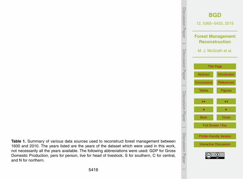
BGD12, 5365–5433, 2015



Title Page



Tables Figures

J I

J I

Back Close

Full Screen / Esc



Discussion

Paper

|D

iscussionP

aper|

Discussion

Paper

|D

iscussionP

aper|

Table 1. Summary of various data sources used to reconstruct forest management between1600 and 2010. The years listed are the years of the dataset which were used in this work,not necessarily all the years available. The following abbreviations were used: GDP for GrossDomestic Production, pers for person, live for head of livestock, S for southern, C for central,and N for northern.

5416





BGD12, 5365–5433, 2015



Title Page



Tables Figures

J I

J I

Back Close

Full Screen / Esc



Discussion

Paper

|D

iscussionP

aper|

Discussion

Paper

|D

iscussionP

aper|

Component Data Comments

GeneralHistorical population maps 1600–2000 Klein Goldewijk et al. (2011); HYDEHistorical GDP data 1600–2000 Bolt and van Zanden (2013); MaddisonWood density 400 kgm−3 Engineering ToolboxCarbon content 50 % Lamlom and Savidge (2003)Charcoal calorific value 30 MJkg−1 Engineering ToolboxWood calorific value 15 MJkg−1 Engineering ToolboxPre-industrial wood to charcoalmass loss ration

4 Menemencioglu (2013); Kammen and Lew (2005)

Fuelwood – CookingEnergy demand 8 GJpers−1 y−1 ASTRA and Reddy (1982)

Upscaled by population. People would use charcoalfor cooking instead of wood for transport and airquality reasons, even if charcoal is less efficient.Energy demand is taken to be similar all over Eu-rope despite differences in diet and climate. It wasassumed that only wood was used as an energysource.

Fuelwood – HeatingTemperature threshold 15.5 ◦C Spinoni et al. (2015)Heating degree days S. Europe 1000 dayK Spinoni et al. (2015)Heating degree days N. Europe 4000 dayK Spinoni et al. (2015)Personal space 30 m3 pers−1 AssumedHeating efficiency 10 % Assumed

Upscaled by population. The energy released whilecooking was used for heating. It was assumed peo-ple would use 50 % charcoal and 50 % wood forheating for transport and air quality reasons, evenif charcoal is less efficient.

5417





BGD12, 5365–5433, 2015



Title Page



Tables Figures

J I

J I

Back Close

Full Screen / Esc



Discussion

Paper

|D

iscussionP

aper|

Discussion

Paper

|D

iscussionP

aper|

Table 1. Continued.


Salt productionWood demand for brineof 250 kgm−3

1 kgkg−1 Radkau (2012)

Wood demand for brineof 50 kgm−3

10 kgkg−1 Radkau (2012)

Production Table 2 Bergier (1989)Upscaled by production. Steady production of the mines throughtime. Brine was transported no more than 25 km throughpipeworks. It was assumed that only wood was used as an en-ergy source.

Beer and distillatesConsumption 300 lpers−1 y−1 Unger (2004)Wood demand 4.8 kgkg−1 Unger (2004)

Upscaled by population. It was assumed that only wood was usedas an energy source.

Ceramics and brickConsumption 45 kgpers−1 y−1 Sinopoli (1999); Petrie (2012)Wood demand 2 kgkg−1 Kishore et al. (2004)

Upscaled by population. It was assumed that only wood was usedas an energy source.

Metal worksIron consumption 1.50 kgpers−1 y−1 Sim and Ridge (2002); Wilson (2007); Craddock (2008);

WikipediaLead consumption 1.45 kgpers−1 y−1 Wilson (2007); WikipediaCopper consumption 0.27 kgpers−1 y−1 Wilson (2007); WikipediaSilver consumption 0.004 kgpers−1 y−1 Wilson (2007); WikipediaGold consumption 0.0002 kgpers−1 y−1 Wilson (2007); WikipediaTin consumption 0.022 kgpers−1 y−1 estimateZinc consumption 0.07 kgpers−1 y−1 estimateWood demand 81 kgkg−1 Sauder and Williams (2002)

Adapted from production estimates from the Roman Empire. Tinand zinc consumption is scaled to copper based on typical bronzeand brass alloys. Upscaled by population. Iron and lead includedmilitary as well as domestic uses. These estimate includes bothmetal melting and working. Wood estimates are prior to charcoalconversion. Charcoal is only mandatory for iron smelting. How-ever, the assumption was made that the preferred fuel for kilnsand furnaces is charcoal because charcoal burns at higher tem-peratures and for ease of transport to production sites.

5418





BGD12, 5365–5433, 2015



Title Page



Tables Figures

J I

J I

Back Close

Full Screen / Esc



Discussion

Paper

|D

iscussionP

aper|

Discussion

Paper

|D

iscussionP

aper|

Table 1. Continued.


Glass productionTotal wood demand forglass

similar to metal works Warde (2006)

Upscaled by metal production. Wood estimates are priorto charcoal conversion and it was assumed only charcoalwas used.

TimberConstruction spendingSpain

18.0×10−5 m3 pers−1 GK−1 Bolt and van Zanden (2013); Iriarte-Goñi and Ayuda(2008)

Construction spendingEngland

7.2×10−5 m3 pers−1 GK−1 Bolt and van Zanden (2013); Clark (2004)

Upscaled by gross domestic production. The share of dif-ferent building materials was assumed constant and a re-lationship between construction and gross domestic pro-duction was assumed.

ShipbuildingShare in wood demand 1 % Warde (2006)

Not accounted for.

Litter rakingLivestock densityN. Europe

0.6 livepers−1 Krausmann et al. (2013)

Livestock densityC. Europe


Livestock densityS. Europe


Litter demand 200–480 kg live−1 y−1 Bürgi (1999)Correction factor1600–1850

LD(y) = 0.75exp(−(y−1850)2/3000)+0.25 Tuned to Bürgi (1999)

Correction factor1851–2010

LD(y) = 1.0exp(−(y −1850)2/1000) Tuned to Bürgi (1999)

Upscaled by population. The correction factor was fittedsuch that agricultural litter use peaked in 1850 and wasabandoned completely by 1950. Northern Europe was de-fined as the land mass above 55◦ N, central Europe waslocated between 45 and 55◦ N and southern Europe theland below 45◦ N. Forage collection was not considered.

5419





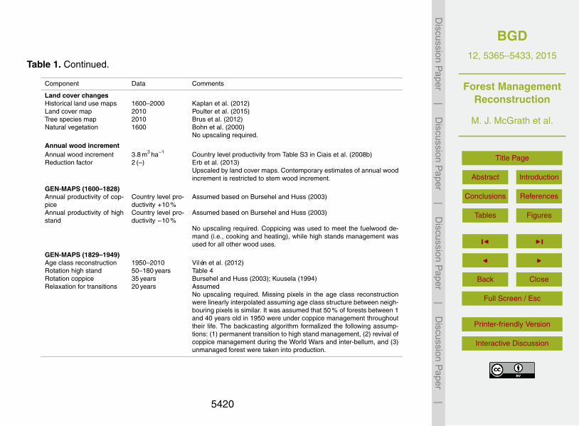
BGD12, 5365–5433, 2015



Title Page



Tables Figures

J I

J I

Back Close

Full Screen / Esc



Discussion

Paper

|D

iscussionP

aper|

Discussion

Paper

|D

iscussionP

aper|

Table 1. Continued.


Land cover changesHistorical land use maps 1600–2000 Kaplan et al. (2012)Land cover map 2010 Poulter et al. (2015)Tree species map 2010 Brus et al. (2012)Natural vegetation 1600 Bohn et al. (2000)

No upscaling required.

Annual wood incrementAnnual wood increment 3.8 m3 ha−1 Country level productivity from Table S3 in Ciais et al. (2008b)Reduction factor 2 (–) Erb et al. (2013)

Upscaled by land cover maps. Contemporary estimates of annual woodincrement is restricted to stem wood increment.

GEN-MAPS (1600–1828)Annual productivity of cop-pice

Country level pro-ductivity +10 %

Assumed based on Bursehel and Huss (2003)

Annual productivity of highstand

Country level pro-ductivity −10 %

Assumed based on Bursehel and Huss (2003)

No upscaling required. Coppicing was used to meet the fuelwood de-mand (i.e., cooking and heating), while high stands management wasused for all other wood uses.

GEN-MAPS (1829–1949)Age class reconstruction 1950–2010 Vilén et al. (2012)Rotation high stand 50–180 years Table 4Rotation coppice 35 years Bursehel and Huss (2003); Kuusela (1994)Relaxation for transitions 20 years Assumed

No upscaling required. Missing pixels in the age class reconstructionwere linearly interpolated assuming age class structure between neigh-bouring pixels is similar. It was assumed that 50 % of forests between 1and 40 years old in 1950 were under coppice management throughouttheir life. The backcasting algorithm formalized the following assump-tions: (1) permanent transition to high stand management, (2) revival ofcoppice management during the World Wars and inter-bellum, and (3)unmanaged forest were taken into production.

5420





BGD12, 5365–5433, 2015



Title Page



Tables Figures

J I

J I

Back Close

Full Screen / Esc



Discussion

Paper

|D

iscussionP

aper|

Discussion

Paper

|D

iscussionP

aper|

Table 1. Continued.


GEN-MAPS (1950–2010)Coppice fraction (1990) 10–50 % Kuusela (1994)Coppice fraction Fenno-Scandinavia (1990)

1 % Assumed based on Emanuelsson (2009)

No upscaling required. All pixels were assumed to contain thesame percentage of coppiced forest area as the country value.The 1990 coppiced areas were held constant until 2010.

ORC-MAPS (1600–2010)General maps 1600–1828 This study, see Sect. 2.4.3General maps 1829–1949 This study, see Sect. 2.4.4General maps 1950–2010 This study, see Sect. 2.4.5Land cover reconstruction 1600–2010 This study, see Sect. 2.3.1Management threshold 15 % AssumedUnmanaged threshold 100 % in 1910 Assumed

15 % by 1950 Assumed based on Schnitzler (2014); Levers et al. (2014)No upscaling required. The demand for wood products from cop-pice management was satisfied before the other wood demands.Dominant PFTs were managed first.

5421





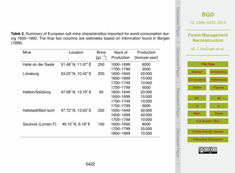
BGD12, 5365–5433, 2015



Title Page



Tables Figures

J I

J I

Back Close

Full Screen / Esc



Discussion

Paper

|D

iscussionP

aper|

Discussion

Paper

|D

iscussionP

aper|

Table 2. Summary of European salt mine characteristics important for wood consumption dur-ing 1600–1900. The final two columns are estimates based on information found in Bergier(1989).

Mine Location Brine Years of Production[gL−1] Production [tonsperyear]

Halle an der Saale 51.48◦ N, 11.97◦ E 250 1600–1699 60001700–1799 3500

Lüneburg 53.25◦ N, 10.42◦ E 250 1600–1649 20 0001650–1699 15 0001700–1749 10 0001750–1799 5000

Hallein/Salzburg 47.68◦ N, 13.10◦ E 50 1600–1649 20 0001650–1699 15 0001700–1749 10 0001750–1799 5000

Hallstadt/Bad Ischl 47.72◦ N, 13.63◦ E 250 1600–1649 50 0001650–1699 40 0001700–1799 10 000

Saulnois (Lorrain F) 49.12◦ N, 6.18◦ E 150 1600–1699 80001700–1799 25 0001800–1899 10 000

5422





BGD12, 5365–5433, 2015



Title Page



Tables Figures

J I

J I

Back Close

Full Screen / Esc



Discussion

Paper

|D

iscussionP

aper|

Discussion

Paper

|D

iscussionP

aper|

Table 3. Summary of independent information, thus not used to create our estimates, for Euro-pean wood demand from around 1600 to 1900.

Summary Source Reconstructed

Fuelwood2–2.5 kgpers−1 day−1 in Northwest and central Europefrom 1500 to 1830.

Warde (2006) 0.9 kgpers−1 day−1

1.4 kgpers−1 day−1 in Madrid in 1680 Warde (2006) 0.9 kgpers−1 day−1

4.7 m3 pers−1 y−1 in Sweden in 1800 Warde (2006) 0.8 m3 pers−1 y−1

1–2.3 m3 pers−1 y−1 in Italy before 1861 Warde (2006) 0.7 m3 pers−1 y−1

Energy demand was 9 GJpers−1 y−1. Fuelwood pres-sure on forests in Switzerland declined by the end of the1800s since coal became used significantly from 1850.

Mather and Fairbairn(2000)

5 GJpers−1 y−1

In Paris, per capita fuelwood consumption amounted1.8 m3 pers−1 y−1 cubic meters in 1815. Fuelwood con-sumption started falling in 1830s in France due to therise of coal.

Mather et al. (1999) 0.9 m3 pers−1 y−1

From 1800, the wood demand was 4 m3 pers−1 y−1 forurban populations in Finland. Wood demand started todecline around 1840.

Myllyntaus and Mat-tila (2002)

0.4 m3 pers−1 y−1

From 1800, the wood demand was 9.5 m3 pers−1 y−1 forrural populations in Finland. Wood demand started todecline around 1840.


0.9 m3 pers−1 y−1

In 1700, 2.3 Tgy−1 of firewood produced in England.Wood had mostly been replaced by coal after 1810 inEngland.

Clark (2004) 1.9 Tgy−1

In 1700, firewood production required 1.83×106 acres(740 000 ha) of coppiced land.

Clark (2004) 1.2×106 ha

5423





BGD12, 5365–5433, 2015



Title Page



Tables Figures

J I

J I

Back Close

Full Screen / Esc



Discussion

Paper

|D

iscussionP

aper|

Discussion

Paper

|D

iscussionP

aper|

Table 3. Continued.

Summary Source Reconstructed

Timber53 % of total wood consumption as sawn tim-ber in Europe in 1920, varying from 15 to96 % of the total wood production based onthe country

Zon and Sparhawk(1923)

N.A.

In Austria the total wood production consistedof 66 % fuelwood in 1877

Weigl (2002) N.A.

In Austria the total wood production consistedof 34 % construction wood in 1877

Weigl (2002) N.A.

Charcoal production30.6×106 feet3 (0.866 Mm3) for iron produc-tion in England in 1700

Clark (2004) 3.8 Mm3

Iron production in England in 1700 required330 000 acres (133 000 ha) of woodland

Clark (2004) 950 000 ha

Total wood demandIn 1800, each Finn consumed20 m3 pers−1 y−1


5 m3 pers−1 y−1

5424





BGD12, 5365–5433, 2015



Title Page



Tables Figures

J I

J I

Back Close

Full Screen / Esc



Discussion

Paper

|D

iscussionP

aper|

Discussion

Paper

|D

iscussionP

aper|

Table 4. Rotation length by tree species and country collected from Kuusela (1994). If an explicityear is not given, the year 1990 (the date of the latest dataset used) is assumed. Region namesare listed in bold font and are defined in Kuusela (1994).

Region/Country Species Years Rotation lengths [years]

Northern Pine 1990 80–120a,c

Spruce 1990 70–90a,c

Pine 1990 110–180b,c

Spruce 1990 90–140b,c

Finland – – –Norway – – –Sweden – – –

CentralDenmark Pine 1990 50–150Germany West Conifers 1920s–1930s 80

Fir 1920s–1930s 90Spruce and fir 1980s 80–100c

Pine and larch 1980s 100–120c

Oak 1980s 140–180Beech 1980s 120–140

Germany East – 1990 “the rotations are somewhat shorter[than those in the rest of the region]”

Poland – 1990 “the rotations are somewhat shorter[than those in the rest of the region]”

Czechoslovakia – 1990 “the rotations are somewhat shorter[than those in the rest of the region]”

Atlantic Pine 1990 50–60Other conifers 1990 50Oak/beech 1990 120–150

Ireland – – –United Kingdom Broadleaf 1990 120

a Southern part of the region.b Northern part of the region.c Actual rotation ages are often 10–20 years longer than prescribed.

5425





BGD12, 5365–5433, 2015



Title Page



Tables Figures

J I

J I

Back Close

Full Screen / Esc



Discussion

Paper

|D

iscussionP

aper|

Discussion

Paper

|D

iscussionP

aper|

Table 4. Continued.


Sub-Atlantic – – –Netherlands – 1990 “rotation ages are relatively short com-

pared with those in Central Europe”Belgium – – –Luxembourg Conifers 1990 80

Broadleaf 1990 130France Broadleaf 1990 140

Spruce and fir 1990 “long rotation”

Alpic – – –Austria – 1990 “relatively long”Switzerland Conifers 1990 80–250

Broadleafs 1990 80–180

Pannonic – – –Hungary Pine 1990 60–70

Other conifers 1990 60–70Oak 1990 90–110, 70–100d

Beech 1990 100–120Poplar 1990 15–30, 15–40d

False acacia 1990 15–30, 30–35 (up to 75)d

Coppice/Coppice with standards 1990 30–75Romania Confiers 1990 100–110, 100–140d

Broadleafs 1990 100–120, 100–140d

d Differing values given at different places in the text.

5426





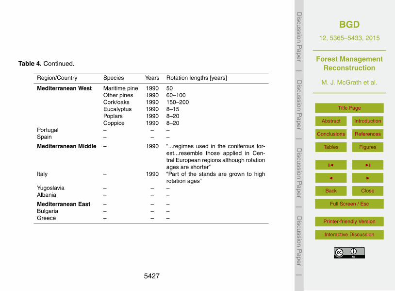
BGD12, 5365–5433, 2015



Title Page



Tables Figures

J I

J I

Back Close

Full Screen / Esc



Discussion

Paper

|D

iscussionP

aper|

Discussion

Paper

|D

iscussionP

aper|

Table 4. Continued.


Mediterranean West Maritime pine 1990 50Other pines 1990 60–100Cork/oaks 1990 150–200Eucalyptus 1990 8–15Poplars 1990 8–20Coppice 1990 8–20

Portugal – – –Spain – – –

Mediterranean Middle – 1990 “...regimes used in the coniferous for-est...resemble those applied in Cen-tral European regions although rotationages are shorter”

Italy – 1990 “Part of the stands are grown to highrotation ages”

Yugoslavia – – –Albania – – –

Mediterranean East – – –Bulgaria – – –Greece – – –

5427





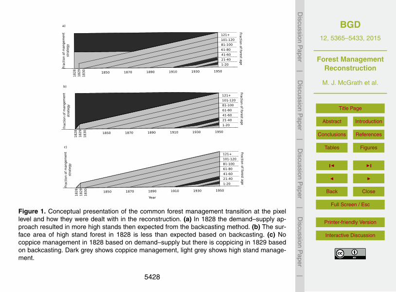
BGD12, 5365–5433, 2015



Title Page



Tables Figures

J I

J I

Back Close

Full Screen / Esc



Discussion

Paper

|D

iscussionP

aper|

Discussion

Paper

|D

iscussionP

aper|

18

30

1850 1870 1890 1910 1930 1950

1-20

21-40

41-60

61-80

81-100

101-120

121+

18

28

Frac

tion

of

man

gem

ent

stra

teg

y

Fraction of forest ag

e

18

29

a)

Year

18

30

1850 1870 1890 1910 1930 1950

1-20

21-40

41-60

61-80

81-100

101-120

121+

18

28

18

29

Frac

tion

of

man

gem

ent

stra

teg

y

b)


e

18

30

1850 1870 1890 1910 1930 1950

1-20

21-40

41-60

61-80

81-100

101-120

121+

18

28

18

29

Frac

tion

of

man

gem

ent

stra

teg

y


e

c)

Figure 1. Conceptual presentation of the common forest management transition at the pixellevel and how they were dealt with in the reconstruction. (a) In 1828 the demand–supply ap-proach resulted in more high stands then expected from the backcasting method. (b) The sur-face area of high stand forest in 1828 is less than expected based on backcasting. (c) Nocoppice management in 1828 based on demand–supply but there is coppicing in 1829 basedon backcasting. Dark grey shows coppice management, light grey shows high stand manage-ment.

5428





BGD12, 5365–5433, 2015



Title Page



Tables Figures

J I

J I

Back Close

Full Screen / Esc



Discussion

Paper

|D

iscussionP

aper|

Discussion

Paper

|D

iscussionP

aper|

1850 1870 1890 1910 1930 1950

Are

a o

f m

angem

en

tst

rate

gy [

ha]

a)

2000

4000

6000

8000

10000

Year

1850 1870 1890 1910 1930 1950

Are

a o

f m

angem

en

tst

rate

gy [

ha]

b)

2000

4000

6000

8000

10000

Figure 2. Conceptual presentation of the common forest management transition at the pixellevel and how they were dealt with in the reconstruction. (a) The amount of coppice area in1850 was higher than what is required in 1950. (b) The amount of coppice area in 1850 waslower than what is required in 1950. Dark grey shows coppice management, light grey showshigh stand management.

5429





BGD12, 5365–5433, 2015



Title Page



Tables Figures

J I

J I

Back Close

Full Screen / Esc



Discussion

Paper

|D

iscussionP

aper|

Discussion

Paper

|D

iscussionP

aper|

Figure 3. Land surface area in 106 km2 covered by forest (blue), grassland (orange), cropland(brown) and bare soil (grey) between 1600 and 2010. The forest area is further separated inconiferous (dark blue) and deciduous (light blue).

5430





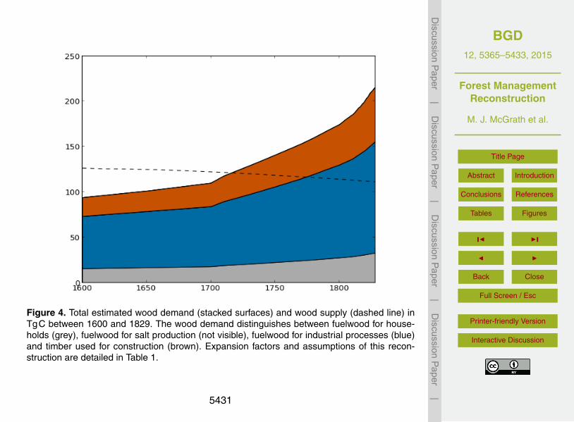
BGD12, 5365–5433, 2015



Title Page



Tables Figures

J I

J I

Back Close

Full Screen / Esc



Discussion

Paper

|D

iscussionP

aper|

Discussion

Paper

|D

iscussionP

aper|

Figure 4. Total estimated wood demand (stacked surfaces) and wood supply (dashed line) inTgC between 1600 and 1829. The wood demand distinguishes between fuelwood for house-holds (grey), fuelwood for salt production (not visible), fuelwood for industrial processes (blue)and timber used for construction (brown). Expansion factors and assumptions of this recon-struction are detailed in Table 1.

5431





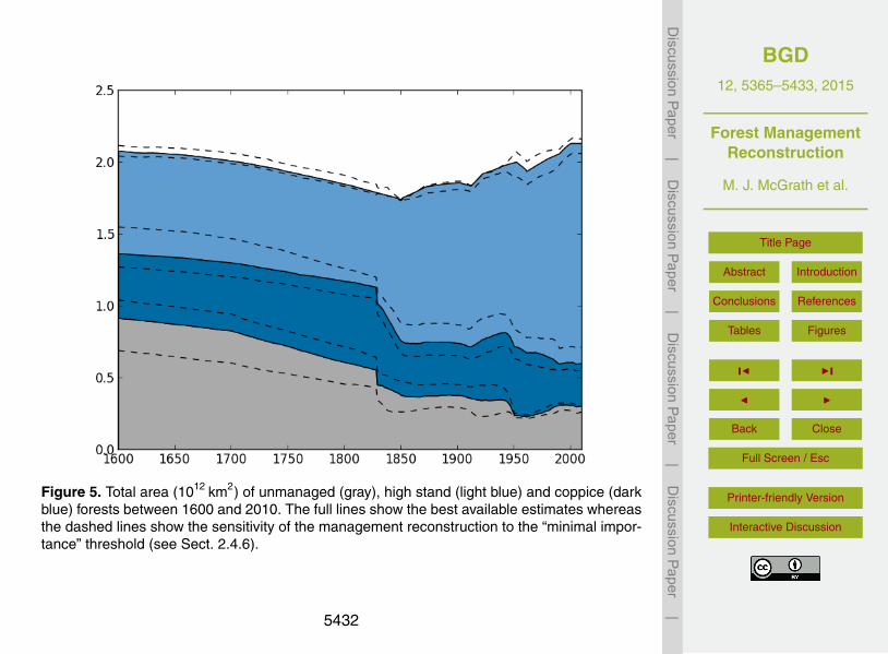
BGD12, 5365–5433, 2015



Title Page



Tables Figures

J I

J I

Back Close

Full Screen / Esc



Discussion

Paper

|D

iscussionP

aper|

Discussion

Paper

|D

iscussionP

aper|

Figure 5. Total area (1012 km2) of unmanaged (gray), high stand (light blue) and coppice (darkblue) forests between 1600 and 2010. The full lines show the best available estimates whereasthe dashed lines show the sensitivity of the management reconstruction to the “minimal impor-tance” threshold (see Sect. 2.4.6).

5432





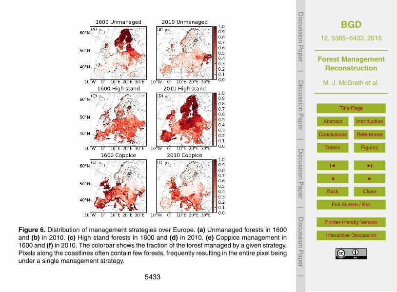
BGD12, 5365–5433, 2015



Title Page



Tables Figures

J I

J I

Back Close

Full Screen / Esc



Discussion

Paper

|D

iscussionP

aper|

Discussion

Paper

|D

iscussionP

aper|

Figure 6. Distribution of management strategies over Europe. (a) Unmanaged forests in 1600and (b) in 2010. (c) High stand forests in 1600 and (d) in 2010. (e) Coppice management in1600 and (f) in 2010. The colorbar shows the fraction of the forest managed by a given strategy.Pixels along the coastlines often contain few forests, frequently resulting in the entire pixel beingunder a single management strategy.

5433





reconstruction of european forest managemnt from 1600 to 2010.pdf

Documents

forest management

todays forest carbon

mcgrath et

surface climate

climate research

climat et lenvironnement

climate service center

land surface models