fmars-07-00464 June 26, 2020 Time: 20:38 # 1

ORIGINAL RESEARCHpublished: 30 June 2020

doi: 10.3389/fmars.2020.00464

Edited by:Juliet Hermes,

South African EnvironmentalObservation Network (SAEON),

South Africa

Reviewed by:Michelle Jillian Devlin,

Centre for Environment, Fisheriesand Aquaculture Science (CEFAS),

United KingdomZhongping Lee,

University of Massachusetts Boston,United States

*Correspondence:Elodie Martinez

elodie.martinez@ird.fr

†††Present address:Matthieu Lengaigne,

MARBEC, University of Montpellier,CNRS, IFREMER, IRD, Sete, France

Raphaëlle Sauzède,CNRS-INSU, Institut de la Mer

de Villefranche, Sorbonne Universités,Villefranche-sur-Mer, France

Specialty section:This article was submitted to

Ocean Observation,a section of the journal

Frontiers in Marine Science

Received: 14 February 2020Accepted: 25 May 2020

Published: 30 June 2020

Citation:Martinez E, Gorgues T,

Lengaigne M, Fontana C, Sauzède R,Menkes C, Uitz J, Di Lorenzo E and

Fablet R (2020) Reconstructing GlobalChlorophyll-a Variations Using

a Non-linear Statistical Approach.Front. Mar. Sci. 7:464.

doi: 10.3389/fmars.2020.00464

Reconstructing Global Chlorophyll-aVariations Using a Non-linearStatistical ApproachElodie Martinez1,2* , Thomas Gorgues1, Matthieu Lengaigne3†, Clement Fontana2,Raphaëlle Sauzède2†, Christophe Menkes4, Julia Uitz5, Emanuele Di Lorenzo6 andRonan Fablet7

1 LOPS, IUEM, IRD, Ifremer, CNRS, Univ. Brest, Brest, France, 2 EIO, IRD, Ifremer, UPF and ILM, Tahiti, French Polynesia,3 LOCEAN-IPSL, Sorbonne Universités/UPMC-CNRS-IRD-MNHN, Paris, France, 4 ENTROPIE (UMR 9220), IRD, Univ. de laRéunion, CNRS, Noumea, New Caledonia, 5 Laboratoire d’Océanographie de Villefranche, CNRS and Sorbonne Université,Villefranche-sur-Mer, France, 6 Georgia Institute of Technology, Atlanta, GA, United States, 7 IMT Atlantique, Lab-STICC,UMR CNRS 6285, Brest, France

Monitoring the spatio-temporal variations of surface chlorophyll-a concentration (Chl, aproxy of phytoplankton biomass) greatly benefited from the availability of continuous andglobal ocean color satellite measurements from 1997 onward. These two decades ofsatellite observations are however still too short to provide a comprehensive descriptionof Chl variations at decadal to multi-decadal timescales. This paper investigates theability of a machine learning approach (a non-linear statistical approach based onSupport Vector Regression, hereafter SVR) to reconstruct global spatio-temporal Chlvariations from selected surface oceanic and atmospheric physical parameters. Witha limited training period (13 years), we first demonstrate that Chl variability from a 32-years global physical-biogeochemical simulation can generally be skillfully reproducedwith a SVR using the model surface variables as input parameters. We then applythe SVR to reconstruct satellite Chl observations using the physical predictors fromthe above numerical model and show that the Chl reconstructed by this SVR moreaccurately reproduces some aspects of observed Chl variability and trends comparedto the model simulation. This SVR is able to reproduce the main modes of interannualChl variations depicted by satellite observations in most regions, including El Niñosignature in the tropical Pacific and Indian Oceans. In stark contrast with the trendssimulated by the biogeochemical model, it also accurately captures spatial patterns ofChl trends estimated by satellite data, with a Chl increase in most extratropical regionsand a Chl decrease in the center of the subtropical gyres, although the amplitude ofthese trends are underestimated by half. Results from our SVR reconstruction overthe entire period (1979–2010) also suggest that the Interdecadal Pacific Oscillationdrives a significant part of decadal Chl variations in both the tropical Pacific and IndianOceans. Overall, this study demonstrates that non-linear statistical reconstructions canbe complementary tools to in situ and satellite observations as well as conventionalphysical-biogeochemical numerical simulations to reconstruct and investigate Chldecadal variability.

Keywords: machine learning, phytoplankton variability, satellite ocean color, decadal variability, global scale

Frontiers in Marine Science | www.frontiersin.org 1 June 2020 | Volume 7 | Article 464

fmars-07-00464 June 26, 2020 Time: 20:38 # 2

Martinez et al. Machine Learning and Reconstruction of Chlorophyll-a Variations

KEY POINTS

1. A machine learning approach is applied to reconstructthe surface phytoplankton biomass at global scaleover three decades.

2. Chlorophyll variability derived from this statisticalapproach accurately reproduces satellite observations(possibly better than biogeochemical models).

3. The sole use of surface predictors allows to accuratelyreproduce chlorophyll variability, in spite of its knownsensitivity to three-dimensional processes.

INTRODUCTION

Phytoplankton—the microalgae that populate the upper lit layersof the ocean—fuels the oceanic food web and regulates oceanicand atmospheric carbon dioxide levels through photosyntheticcarbon fixation. The launch of the “Coastal Zone ColorScanner” (CZCS) onboard the Nimbus-7 spacecraft in October1978 (Hovis et al., 1980) provided the first synoptic viewof near-surface chlorophyll-a concentration (Chl, a proxy ofphytoplankton biomass). Although primarily focusing on coastalregions, CZCS also provided global pictures of Chl distributionand a new perspective on phytoplankton biomass seasonalvariability (Campbell and Aarup, 1992; Longhurst et al., 1995;Yoo and Son, 1998; Banse and English, 2000).

After the failure of CZCS in 1986, ocean color observationswere not available for more than a decade. The launch ofthe modern radiometric Sea-viewing Wide Field-of-View Sensor(SeaWiFS; McClain et al., 2004) in late 1997 followed laterby other satellites allowed monitoring and understanding thespatio-temporal Chl variations at global scale over the past twodecades. For instance, it revealed that El Niño events induce a Chldecrease in the central and eastern equatorial Pacific in responseto reduced upwelled nutrients to the surface layers (e.g., Chavezet al., 1999; Wilson and Adamec, 2001; McClain et al., 2002;Radenac et al., 2012) but also a Chl signature outside the tropicalPacific through atmospheric teleconnections (Behrenfeld et al.,2001; Yoder and Kennelly, 2003; Dandonneau et al., 2004; Messiéand Chavez, 2012). It also allowed identifying the Indian OceanDipole (IOD; Saji et al., 1999) as the main climate mode drivingChl interannual variations in the Indian Ocean (e.g., Murtuguddeet al., 1999; Wiggert et al., 2009; Currie et al., 2013) andmonitoring a Chl increase in the subpolar North Atlantic relatedto the positive phase of the North Atlantic Oscillation (NAO)(Martinez et al., 2016). Aside from the Chl decrease monitoredin the mid-ocean gyres over the first decade of the XXIst century(Polovina et al., 2008; Irwin and Oliver, 2009; Vantrepotte andMélin, 2009; Signorini and McClain, 2012), the reliability ofthe long-term trends derived from these satellite data are morequestionable and led to conflicting results in the past literature(Behrenfeld et al., 2006; Vantrepotte and Mélin, 2011; Siegel et al.,2013; Gregg and Rousseaux, 2014). These discrepancies suggestthat detection of robust global trend may require several decadesof continuous observations (Beaulieu et al., 2013).

The production of longer, consistent ocean color time seriescan partly alleviate this issue. The combination of the globalCZCS and SeaWiFS datasets provided an insight on the Chlresponse to natural decadal climate variations (Martinez et al.,2009; D’Ortenzio et al., 2012), such as the Pacific DecadalOscillation (PDO; Mantua et al., 1997) and the AtlanticMultidecadal Oscillation (AMO; Enfield et al., 2001). However,blending these two archives or reconstructing them usingcompatible algorithms also led to contrasting results (Gregg andConkright, 2002; Antoine et al., 2005).

The time span of the modern radiometric observations(∼20 years), as well as the CZCS-SeaWiFS reprocessed timeseries, are still too short to investigate Chl decadal variations andlonger-term trends. Longer, continuous and consistent recordsare required. In situ biogeochemical observatories can providesuch long and continuous records, but their inhomogeneousspatial distribution and varying record length prevent a confidentassessment of Chl long-term changes at the scale of a basin(Henson et al., 2016).

Coupled physical-biogeochemical ocean model simulationscan provide additional, valuable information’s in areas withlimited observational coverage. These models resolve reasonablywell the seasonal to interannual biogeochemical variability(Dutkiewicz et al., 2001; Wiggert et al., 2006; Aumont et al.,2015). They can however diverge in capturing Chl variations at atimescale of a decade (Henson et al., 2009a,b; Patara et al., 2011),in particular phytoplankton regime shifts (Henson et al., 2009b).Different biological models are often coupled to different physicalmodels, which renders the attribution of the different modeledresponses to their physical or biological components difficult. Thedecadal or longer variability of the simulated primary producersshould then be interpreted cautiously.

In this context, statistical methods reconstructing past Chlvariations may be useful alternatives to overcome limitationsassociated with both observations and numerical models. Whilestatistical reconstructions are now commonly used to extendphysical variables back in time (e.g., Smith et al., 2012; Huanget al., 2017; Nidheesh et al., 2017), reconstructions of surface Chlare still in their infancy. Phytoplankton distribution is stronglycontrolled by physical processes, such as mixing and uplifting,fueling nutrients in the upper-lit layer (i.e., bottom up processes).Thus, relevant physical variables may allow to reconstruct Chlpast variations. To our knowledge, a single study allowed thederivation of spatio-temporal surface Chl variations over severaldecades in the tropical Pacific (Schollaert Uz et al., 2017). Thisreconstruction used a linear canonical correlation analysis onSea Surface Temperature (SST) and Sea Surface Height (SSH) toimprove the description of the Chl response to the diversity ofobserved El Niño events and decadal climate variations in thetropical Pacific.

The objective of the present study is to explore the potentialof an alternative statistical technique to reconstruct Chl atglobal scale over a 32-year time-series (i.e., 1979–2010). Theconsidered machine learning technique is based on a SupportVector Regression (SVR) which accounts for non-linearitiesbetween predictors and Chl. First, the SVR is trained over 1998–2010 on a self-consistent dataset of physical and Chl variables,

Frontiers in Marine Science | www.frontiersin.org 2 June 2020 | Volume 7 | Article 464

fmars-07-00464 June 26, 2020 Time: 20:38 # 3

Martinez et al. Machine Learning and Reconstruction of Chlorophyll-a Variations

all extracted from a forced ocean model simulation that includesa biogeochemical component (i.e., the NEMO-PISCES model).Then, modeled physical variables are used to reconstruct Chlover 1979–2010. The feasibility and robustness of the proposedreconstruction process is assessed through the comparison ofmodeled vs. reconstructed Chl. In a second step, this frameworkis applied to satellite ocean color observations.

DATA AND METHODS

The NEMO-PISCES SimulationIn this study, we used the “Nucleus for European Modelingof the Ocean” (NEMO) modeling framework (Madec,2008). The NEMO configuration used displays a coarseresolution with 31 vertical levels and a 2◦ horizontal gridwith a refined 0.5◦ resolution in the equatorial band. Themodel includes a biogeochemical component, the PelagicInteraction Scheme for Carbon and Ecosystem Studies (PISCES;Aumont et al., 2015). PISCES is a model of intermediatecomplexity designed for global ocean applications (Aumontand Bopp, 2006), which uses 24 prognostic variables andsimulates biogeochemical cycles of oxygen, carbon and themain nutrients controlling phytoplankton growth (nitrate,ammonium, phosphate, silicic acid, and iron). It simulates thelower trophic levels of marine ecosystems distinguishing fourplankton functional types based on size: two phytoplanktongroups (small = nanophytoplankton and large = diatoms)and two zooplankton groups (small = microzooplankton andlarge = mesozooplankton). Chl from PISCES (hereafter referredto as ChlPISCES) is defined as the sum of the simulated diatomsand nanophytoplankton Chl content.

The NEMO-PISCES simulation is forced with atmosphericfields from the interannual Drakkar Forcing Set 5 (DFS5.2,Dussin et al., 2014) for wind, air temperature and humidity,precipitation, shortwave and longwave radiations. It is initializedwith the World Ocean Atlas 2005 (WOA05) climatology fortemperature, salinity, phosphate, nitrate and silicate (Garcia et al.,2006), while iron initial state is similar to the model climatologyemployed by Aumont and Bopp (2006). The model simulationwas spun up using 3 repetitions of the 30 years’ DFS5.2 forcingset, and finally ran over 1979–2010.

Although successfully used in a variety of biogeochemicalstudies (e.g., Bopp et al., 2005; Gehlen et al., 2006; Lengaigne et al.,2007; Schneider et al., 2008; Steinacher et al., 2010; Tagliabueet al., 2010; Séférian et al., 2013; Aumont et al., 2015; Keerthiet al., 2017; Parvathi et al., 2017 and references therein), the abilityof the PISCES model to reproduce satellite surface Chl is brieflyillustrated in section “Evaluation of ChlPISCES at global scale.”

Chl Derived From Satellite RadiometricObservationsSatellite surface Chl for Case I waters is provided by the OceanColor – Climate Change Initiative (OC-CCI, hereafter referredto as ChlOC−CCI) from the European Space Agency1. This

1http://www.esaoceancolour-cci.org/

product combines multi-sensor, global, ocean-color productswhile attempting to reduce inter-sensor biases for climateresearch (Storm et al., 2013). OC-CCI extends the time seriesbeyond that provided by single satellite sensors and is performantin terms of long-term consistency than other products frommulti-mission initiatives (Belo Couto et al., 2016).

Only deep oceanic areas (depth > 200 m) are consideredto avoid coastal waters where specific non-case-1 watersproducts are required. The Chl Level-3 product is binned on aregular 1◦ grid with a monthly resolution over January 1998–December 2010. This time period does not extend beyond2010 to be consistent with the NEMO-PISCES simulation.ChlOC−CCI is used to evaluate the PISCES model performancesin Section “Evaluation of ChlPISCES at global scale,” and totrain the statistical method in Section “Application to satelliteradiometric observations.”

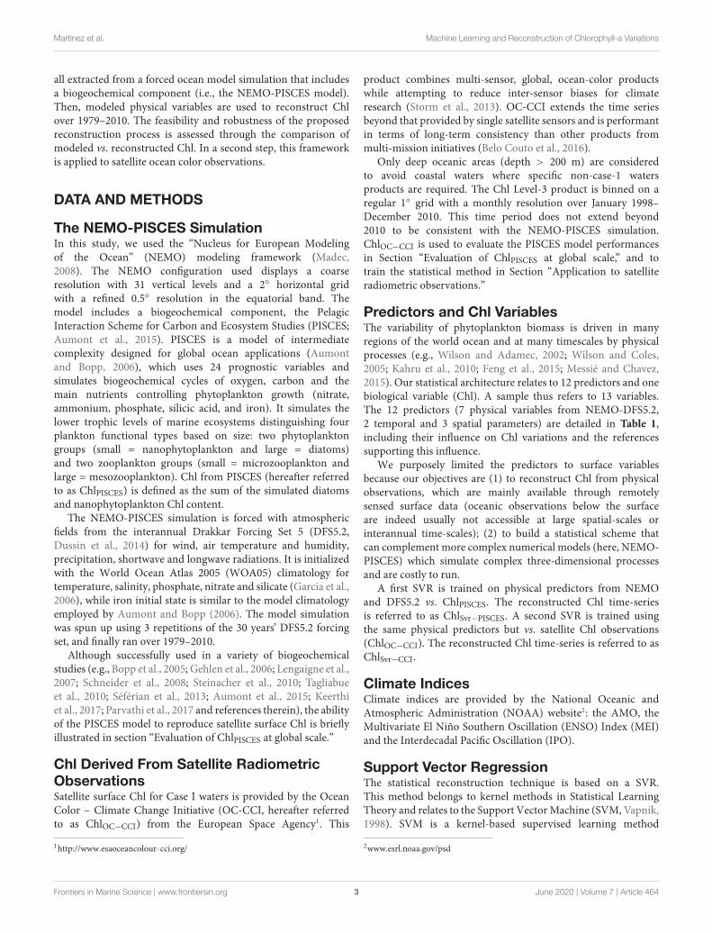
Predictors and Chl VariablesThe variability of phytoplankton biomass is driven in manyregions of the world ocean and at many timescales by physicalprocesses (e.g., Wilson and Adamec, 2002; Wilson and Coles,2005; Kahru et al., 2010; Feng et al., 2015; Messié and Chavez,2015). Our statistical architecture relates to 12 predictors and onebiological variable (Chl). A sample thus refers to 13 variables.The 12 predictors (7 physical variables from NEMO-DFS5.2,2 temporal and 3 spatial parameters) are detailed in Table 1,including their influence on Chl variations and the referencessupporting this influence.

We purposely limited the predictors to surface variablesbecause our objectives are (1) to reconstruct Chl from physicalobservations, which are mainly available through remotelysensed surface data (oceanic observations below the surfaceare indeed usually not accessible at large spatial-scales orinterannual time-scales); (2) to build a statistical scheme thatcan complement more complex numerical models (here, NEMO-PISCES) which simulate complex three-dimensional processesand are costly to run.

A first SVR is trained on physical predictors from NEMOand DFS5.2 vs. ChlPISCES. The reconstructed Chl time-seriesis referred to as ChlSvr−PISCES. A second SVR is trained usingthe same physical predictors but vs. satellite Chl observations(ChlOC−CCI). The reconstructed Chl time-series is referred to asChlSvr−CCI.

Climate IndicesClimate indices are provided by the National Oceanic andAtmospheric Administration (NOAA) website2: the AMO, theMultivariate El Niño Southern Oscillation (ENSO) Index (MEI)and the Interdecadal Pacific Oscillation (IPO).

Support Vector RegressionThe statistical reconstruction technique is based on a SVR.This method belongs to kernel methods in Statistical LearningTheory and relates to the Support Vector Machine (SVM, Vapnik,1998). SVM is a kernel-based supervised learning method

2www.esrl.noaa.gov/psd

Frontiers in Marine Science | www.frontiersin.org 3 June 2020 | Volume 7 | Article 464

fmars-07-00464 June 26, 2020 Time: 20:38 # 4

Martinez et al. Machine Learning and Reconstruction of Chlorophyll-a Variations

TABLE 1 | Physical predictors, their relevance to Chl variations and associated references.

Proxy used as predictors Relevance to Chl variations References

SST Vertical mixing and upwelling Impacts on phytoplanktonmetabolic rates

Behrenfeld et al., 2006; Polovina et al., 2008; Martinezet al., 2009; Thomas et al., 2012; Lewandowska et al.,2014

Sea level anomaly Thermocline/pycnocline depths Wilson and Adamec, 2001, 2002; Radenac et al., 2012

Zonal and meridional surface windcomponents

Surface momentum flux forcing and vertical motions drivenby Ekman pumping

Martinez et al., 2011; Thomas et al., 2012

Zonal and meridional surfacecurrent components

Horizontal advective processes Messié and Chavez, 2012; Radenac et al., 2013

Short-wave radiations Photosynthetically active radiation Sakamoto et al., 2011

Month (cos and sin) Periodicity of the day of the year (day 1 is very similar to day365 from a seasonal perspective)

Sauzède et al., 2015

Longitude (cos and sin) Latitude (sin) Periodicity (longitude 0◦ = longitude 360◦) Sauzède et al., 2015

(Vapnik, 2000) developed for classification purpose in the early1990s and then extended for regression by Vapnik (1995). Thebasic idea behind SVR is to map the variables into a new non-linear space using the kernel function, so that the regressiontask becomes linear in this space. The learning step estimatesthe parameters of the regression model according to a linearquadratic optimization problem, which can be solved efficiently.SVR also uses a robust error norm based on the principle ofstructural risk minimization, where both the error rates and themodel complexity should be minimized simultaneously. BecauseSVR can efficiently capture complex non-linear relationships,it has been used in a variety of fields, and more specificallyfor oceanographic, meteorological and climate impact studies(Aguilar-Martinez and Hsieh, 2009; Descloux et al., 2012; Elbisy,2015; Neetu et al., 2020), as well as in marine bio-optics (Kimet al., 2014; Hu et al., 2018; Tang et al., 2019).

Predictors and Chl are normalized by removing theirrespective average and dividing them by their standarddeviations. Two SVR are trained over 1998-2010: one onChlPISCES and one on ChlOC−CCI (Step A in Figure 1). This timeperiod has been chosen as 1998 is the first complete year of thesatellite ChlOC−CCI time-series, and 2010 is the last year availableof the modeled ChlPISCES. The two resulting SVR schemesare applied on the NEMO-DFS5.2 physical predictors over1979–2010. Finally, the annual means and standard deviationsinitially removed are applied to perform the back transformationand reconstruct either ChlSvr−PISCES or ChlSvr−CCI (Step Bin Figure 1).

Considering a Gaussian kernel, SVR only involves theselection of two hyperparameters: the penalty parameter C ofthe error term and the kernel coefficient gamma, driving thereduction of the cost function. C and gamma values are 1 and 0.1,respectively when the SVR is trained on ChlPISCES, and 2 and 0.3when trained on ChlOC−CCI (see details in the SupplementaryMaterial and Supplementary Figure 1A). Sensitivity tests to anincreasing portion of the sample total number (from 0.2 to 9% ofthe full dataset) used in the training process are performed (seeSupplementary Material and Supplementary Figure 1B). Themean absolute error stabilizes for a sample number higher than6%, suggesting that the SVR skills don’t improve much afterward.This observation combined with computational limitations leadus to present the 9% experiment hereafter.

Empirical Orthogonal Function AnalysisThe SVR skills to reconstruct Chl interannual to decadalvariations are investigated performing Empirical OrthogonalFunction analysis on ChlPISCES, ChlOC−CCI, ChlSvr−PISCES andChlSvr−CCI. First, Chl data are centered and reduced (i.e., themonthly climatology is removed and the induced anomaliesare divided by their standard deviations) to avoid an overlydominant contribution of high values on the analysis (Emeryand Thomson, 1997) over the periods of interest (i.e., 1998–2010 or 1979–2010). A 5-month running mean is appliedto focus on the interannual/decadal signal. The analysis isseparately performed for the Atlantic, Pacific and Indian Oceansnorth of 40◦S until 60◦N, and for the 40◦S–60◦S regionhereafter referred to as the Austral Ocean. Indeed, the largearea covered by the Pacific Ocean and its dominant modes inclimate variability (i.e., ENSO/IPO), could regionally dampenother modes of variability. Basin-scale spatial maps are thengathered to a global one, referred to as EOF. The associatedtime-series refer to as the Principal Components (PCs).

SYNTHETIC RECONSTRUCTION FROMA PHYSICAL-BIOGEOCHEMICALOCEAN MODEL

This section assesses the reliability and robustness of the SVRapproach using a complete and coherent dataset extractedfrom a global simulation performed with a coupled physical-biogeochemical ocean model. The SVR is first trained over1998–2010 on ChlPISCES, and ChlSvr−PISCES is reconstructed over1979–2010. ChlPISCES and ChlSvr−PISCES are then compared over32 years to evaluate the consistency of the proposed data-drivenreconstruction scheme.

Evaluation of ChlPISCES at Global ScaleThe ability of the NEMO-PISCES model to reproduce the satelliteChl over 1998–2010 is briefly presented here. Boreal winterand summer climatology from ChlPISCES compare reasonablywell with those of ChlOC−CCI (Figure 2A vs. 2B and 2C vs.2D). The model correctly represents the main spatial patternswith, for instance, higher Chl and a stronger seasonal cycle

Frontiers in Marine Science | www.frontiersin.org 4 June 2020 | Volume 7 | Article 464

fmars-07-00464 June 26, 2020 Time: 20:38 # 5

Martinez et al. Machine Learning and Reconstruction of Chlorophyll-a Variations

FIGURE 1 | Steps performed to train the SVR and reconstruct Chl time-series.

at high latitudes, despite an overestimated biomass in theSouthern Ocean (Launois et al., 2015). The model also captureslow Chl in the subtropical gyres, with some underestimation.This discrepancy may be explained by the lack of acclimationdynamics to oligotrophic conditions or by the assumption ofconstant stoichiometry either in phytoplankton or in organicmatter in the model (Ayata et al., 2013; Aumont et al., 2015). Themodel underestimates Chl values in the equatorial Atlantic andArabian Sea. In this latter region, mesoscale and submesoscaleprocesses unresolved by the model have been shown to be ofcritical importance (Hood et al., 2003; Resplandy et al., 2011).Finally, the parameterization of nitrogen-fixing organisms notexplicitly modeled in that PISCES version could explain theChlPISCES underestimation in the western Pacific in australsummer (Dutheil et al., 2018).

High Chl are accurately simulated in the eastern boundaryupwelling systems. In two of the three main High Nutrient LowChlorophyll (HNLC) regions, i.e. the equatorial Pacific andthe eastern subarctic Pacific, the model successfully reproducesthe moderate ChlOC−CCI. However, the model overestimatesChlOC−CCI east of Japan because of an incorrect representationof the Kuroshio current trajectory. This common bias in coarseresolution models (i.e., Gnanadesikan et al., 2002; Dutkiewiczet al., 2005; Aumont and Bopp, 2006) is potentially relatedto too deep mixed layer simulated in winter inducing verystrong spring blooms (Aumont et al., 2015). In the SouthernOcean, the third and largest main HNLC region, the modeloverestimates ChlOC−CCI values, especially during summer.However, the standard satellite algorithms that deduce Chlfrom reflectance tend to underestimate in situ observations by afactor of about 2–2.5, especially for intermediate concentrations

(e.g., Dierssen and Smith, 2000; Kahru and Mitchell, 2010).It is to note that Chl in physical-biogeochemical coupledmodels is commonly overestimated in the Southern Ocean,and systematically underestimated in the oligotrophic gyres(Séférian et al., 2013).

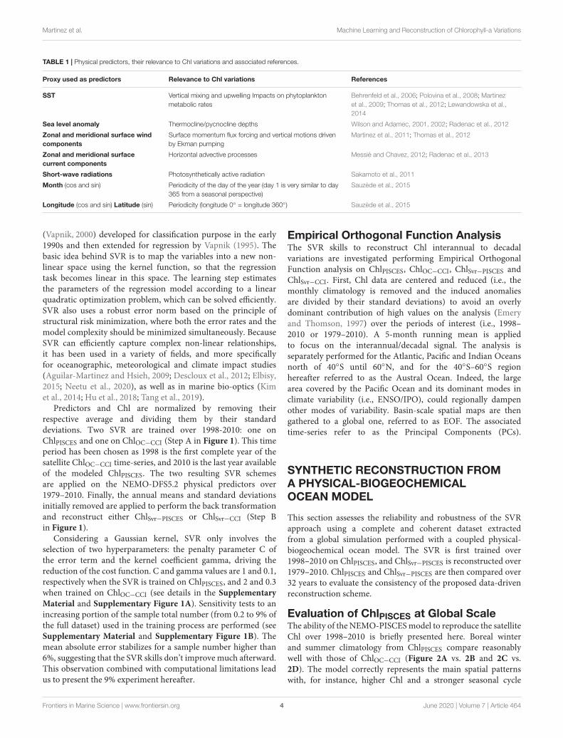
The 1st mode of the EOF analysis performed on interannualChl displays close percent of total variance for ChlOC−CCI andChlPISCES (16.6% vs. 21.1%, respectively). Their PCs in the PacificOcean are well correlated with the MEI (r = 0.71 and 0.89with p = 0.0015 and p < 0.001, respectively; Figure 3C). PCsshow the greatest positive values in January 1998 during thepeak of the strong 1997/1998 El Niño event and the greatestnegative values during the following La Niña beginning of1999. The associated EOFs display a Chl horseshoe pattern(Figures 3A,B), reminiscent of the ENSO pattern on SST(Supplementary Figure 2; Messié and Chavez, 2012). While thetropical Pacific experiences a Chl decrease during El Niño events,the North and South Pacific display a Chl increase, and inverselyduring La Niña. This typical ENSO pattern is also related toremote Chl anomalies outside the Pacific induced by atmosphericteleconnections, such as a Chl decrease in the tropical NorthAtlantic and in the South Indian Ocean during El Niño. Althoughthe Atlantic and Indian Ocean’s PCs are not correlated withthe MEI (0.14 and 0.05, respectively), their EOFs are similarto those obtained from analysis performed at global scale (vs.basin scale here) and which have been largely discussed in thepast (e.g., Behrenfeld et al., 2001, 2006; Yoder and Kennelly,2003; Chavez et al., 2011). ChlPISCES reasonably well capturesthe first mode of ChlOC−CCI interannual variability over 1998–2010 in the Pacific and Atlantic Oceans, with 0.89 and 0.77(p < 0.001) correlations between their PCs, respectively, but not

Frontiers in Marine Science | www.frontiersin.org 5 June 2020 | Volume 7 | Article 464

fmars-07-00464 June 26, 2020 Time: 20:38 # 6

Martinez et al. Machine Learning and Reconstruction of Chlorophyll-a Variations

FIGURE 2 | Surface seasonal mean of Chl (mg.m−3) over 1998–2010 derived from satellite (left panels) and the PISCES model (right panels), inOctober–November–December (A,B) and April–May–June (C,D).

in the Indian Ocean, where the PCs correlation is far weaker(0.13) and insignificant (Figures 3C–E).

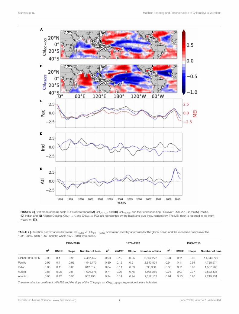
Evaluation of the SVR Method Trained onSynthetic Data OnlyStatistical PerformancesA first evaluation of the SVR applied on the synthetic dataset (i.e.,both physical and biogeochemical model outputs) is provided forthe dedicated subset (i.e., 20% of 9% of the total data set) overthe 1998–2010 training time period. ChlPISCES and ChlSvr−PISCESdatasets display a determination coefficient of 0.95 and aroot mean square error (RMSE) of 0.22 (see SupplementaryFigure 1C), indicating at first glance a very good ability of theSVR to reconstruct ChlPISCES. The SVR reconstruction is veryaccurate when comparing the full modeled and reconstructed Chlfor (i) the 1998–2010 training time period, (ii) the 1979–1997fully independent dataset, and (iii) the 1979–2010 whole dataset,both at global and basin scales (Table 2 and Figure 4). For eachoceanic basin, determination coefficients between both datasetsover 1979–1997 exceed 0.84, except in the Austral Ocean wherethey get down to 0.71. RMSE are lower than 0.14 and associatedwith a slope ranging from 0.84 in the Austral to 0.97 in theAtlantic (Figure 4). In addition, the quality of the reconstructedChlSvr−PISCES over the 1979–1997 independent time period isonly marginally degraded compared to the 1998–2010 trainingperiod or the 1979–2010 full period.

Evaluation of the Reconstructed Chl Spatio-TemporalVariabilityThe Normalized Root-Mean-Square-Error (NRMSE, i.e., RMSEnormalized by the average Chl used to train the SVR) betweenChlPISCES and ChlSvr−PISCES filtered with a 5-month runningmean (to discard the high frequency signal) shows an errorranging between 10 and 20% over 1998–2010 (Figure 5A). Theircorrelation exceeds 0.7 (p < 0.001) over most of the globalocean (Figure 5B). At mid-latitudes they are generally largerthan 0.8, and they range between 0.6 and 0.9 in the equatorialPacific. This accurate reconstruction demonstrates that a strongrelationship exists between physical processes and Chl at globalscale. However, the reconstructed Chl field can be regionallyless accurate. For instance, the edges of the oligotrophic gyres(delimited by the 0.1 mg.m−3 contour in Figure 5A) exhibitthe highest NRMSE and lowest correlations. Large NRMSE arealso evident in the Gulf Stream region while the western tropicalAtlantic exhibits lower correlations than 0.5.

Those discrepancies could be due first to the zooplanktongrazing pressure (top–down control) which is oftenoverestimated in PISCES simulations. It results in anunderestimated nanophytoplankton biomass in the oligotrophicgyres, emphasized along their edges (Laufkötter et al., 2015).Because the top–down control is not accounted for by theSVR, Chl variability induced by the overgrazing in theseareas might not be captured. Second, in the equatorial PacificOcean, a minimum iron threshold value has been imposed

Frontiers in Marine Science | www.frontiersin.org 6 June 2020 | Volume 7 | Article 464

fmars-07-00464 June 26, 2020 Time: 20:38 # 7

Martinez et al. Machine Learning and Reconstruction of Chlorophyll-a Variations

FIGURE 3 | First mode of basin-scale EOFs of interannual (A) ChlOC−CCI and (B) ChlPISCES, and their corresponding PCs over 1998–2010 in the (C) Pacific,(D) Indian and (E) Atlantic Oceans. ChlOC−CCI and ChlPISCES PCs are represented by the black and blue lines, respectively. The MEI index is reported in red (righty-axis) on (C).

TABLE 2 | Statistical performances between ChlPISCES vs. ChlSvr−PISCES normalized monthly anomalies for the global ocean and the 4 oceanic basins over the1998–2010, 1979–1997, and the whole 1979–2010 time period.

1998–2010 1979–1997 1979–2010

R2 RMSE Slope Number of bins R2 RMSE Slope Number of bins R2 RMSE Slope Number of bins

Global 60◦S-60◦N 0.96 0.1 0.95 4,487,457 0.93 0.12 0.95 6,562,272 0.94 0.11 0.95 11,049,729

Pacific 0.92 0.1 0.93 1,945,173 0.89 0.12 0.9 2,843,501 0.9 0.11 0.91 4,788,674

Indian 0.86 0.11 0.85 612,612 0.84 0.11 0.89 895,356 0.85 0.11 0.87 1,507,968

Austral 0.81 0.06 0.8 1,026,876 0.71 0.08 0.75 1,506,260 0.76 0.07 0.77 2,533,136

Atlantic 0.96 0.12 0.96 902,796 0.94 0.14 0.94 1,317,155 0.94 0.13 0.95 2,219,951

The determination coefficient, NRMSE and the slope of the ChlPISCES vs. ChlSvr−PISCES regression line are indicated.

Frontiers in Marine Science | www.frontiersin.org 7 June 2020 | Volume 7 | Article 464

fmars-07-00464 June 26, 2020 Time: 20:38 # 8

Martinez et al. Machine Learning and Reconstruction of Chlorophyll-a Variations

FIGURE 4 | Scatter plots of ChlPISCES vs. ChlSvr−PISCES normalized monthly anomalies over 1979–1997, (A–D) for each basin and (E) at global scale between 60◦Sand 60◦N. The ChlPISCES vs. ChlSvr−PISCES and the 1:1 regression lines are plotted as the continuous red and dash black lines, respectively. The figure is color-codedaccording to the density of observations.

FIGURE 5 | (A,B) NRMSE (in%) and (C,D) correlation between ChlPISCES vs. ChlSvr−PISCES after applying a 5 month-running mean on both time-series. These 2diagnostics are calculated over 1998–2010 (left column) and 1979–1997 (right column). Contours on the upper panels show their respective 1998–2010 Chl timeaverage (every 0.1 mg.m−3).

(0.01 nmol.L−1) in the biogeochemical model. Without thatthreshold Chl is too low on both sides of the equator, resultingin a strong accumulation of macronutrients and a spuriouspoleward migration of the subtropical gyre boundaries (Aumontet al., 2015). While the existence of such a threshold suggests thata minor but regionally important source of iron is missing in

PISCES, it also suggests the inability of the SVR in reproducingecosystem dynamics related to such artificial input of micro-nutrient. Finally, atmospheric input of iron through desertdust deposition is known to be stronger in the Atlantic thanin the Pacific Ocean (Jickells et al., 2005). Such signal cannotbe accounted for by the SVR with the given predictors, which

Frontiers in Marine Science | www.frontiersin.org 8 June 2020 | Volume 7 | Article 464

fmars-07-00464 June 26, 2020 Time: 20:38 # 9

Martinez et al. Machine Learning and Reconstruction of Chlorophyll-a Variations

might (with meso – and sub-mesoscale activities) explainthe higher NRMSE in the north western Atlantic than in thenorth-western Pacific.

As expected, areas of high NRMSE and low correlationsbetween ChlPISCES and ChlSvr−PISCES identified over 1998–2010(Figure 5, left column) extend and strengthen over 1979–1997(Figure 5, right column). Indeed, the correlations significantlydecrease in the tropical Pacific while they slightly decrease in mid-latitudes between the two periods. Correlations remain high andNRMSE low in the North-West Pacific, North and South-WestAtlantic, and South Indian Oceans as well as over a large part ofthe Southern Ocean providing confidence for analyses extendedbeyond the training period of the SVR.

The analysis is now extended to the 1979–2010 time-period to investigate the skills of the SVR in reproducingphytoplankton interannual/decadal cycles. The 1st EOFs ofChlPISCES vs. ChlSvr−PISCES have the same sign of variabilityover 72% of the global ocean (Figures 6A,B). Both EOFs aresimilar in the Pacific and Atlantic Oceans and their PCs arehighly correlated over 1979-2010 (Table 3 and Figures 6C,E). Inthe Pacific, these EOFs strongly resemble the typical horseshoepattern of IPO with SST anomalies of opposite polarities inthe tropical and extra-tropical Pacific regions (SupplementaryFigure 3). Correlations between ChlPISCES and ChlSvr−PISCES 1stPCs and the IPO index are high (0.94 and 0.95 with p < 0.001,respectively; blue and black vs. red lines in Figure 6C). Ithighlights that the 1st mode of Chl variability in the Pacificis strongly driven by the IPO. In the Atlantic, both PCs arestrongly correlated with the AMO (−0.8 for ChlSvr−PISCESand −0.85 for ChlPISCES with p < 0.001; Figure 6E). TheAMO shifts from a cold to a warm phase in the mid-1990’s(Supplementary Figure 3), and is associated with a decrease inChl (Figures 6A,B).

The 1st two modes explain a similar percent variance forChlPISCES and ChlSvr−PISCES in the four oceanic basins, with theexception of the 1st mode in the Atlantic Ocean (see Table 3). Inthis basin ChlSvr−PISCES percent variance is underestimated by afactor 2 compared to ChlPISCES, while their 1st EOFs and PCs arewell correlated. One explanation might be that the AMO is theclimate cycle with the longest period (80 years) when compared tothe IPO. Thus, it might be the most difficult signal to reproduce asthe SVR is trained over a relatively “short” 12 years’ time-period.

The agreement between ChlPISCES and ChlSvr−PISCES1st mode is not as good in the Austral and Indian Oceans

when compared to the Atlantic and Pacific Oceans(Table 3 and Figures 6A,B,D,F). In the Indian Ocean, theChlPISCES EOF exhibits a maximum positive variabilityalong the western Arabian Sea, while it is located north-east of Madagascar for ChlSvr−PISCES. In the AustralOcean, ChlPISCES and ChlSvr−PISCES EOFs roughly follow azonal distribution.

A strong correspondence between SST and Chl has beenpreviously reported over a large part of the global ocean(Behrenfeld et al., 2006; Martinez et al., 2009; Siegel et al.,2013), demonstrating the close interrelationship betweenocean biology and climate variations. Consequently, it is notsurprising to observe strong correlations between ChlPISCES orChlSvr−PISCES and climatic indexes mostly built on SST anomalies(Supplementary Figure 3).

The 2nd mode of variability of ChlPISCES is also wellreproduced by the SVR. The percent variances are close (Table 3)as well as their spatio-temporal variability in the four oceanicbasins (Supplementary Figure 4). The high correlations betweenthe first two modes of ChlPISCES vs. ChlSvr−PISCES highlightthe SVR ability to relatively well reproduce the ChlPISCES low-frequency variability.

APPLICATION TO SATELLITERADIOMETRIC OBSERVATIONS

SVR Statistical Performances andSensitivity TestsIn this section, the SVR uses the same physical predictors fromNEMO-DFS5.2 as in Section “Synthetic reconstruction froma physical-biogeochemical ocean model,” but it is trainedon satellite radiometric observations (e.g., ChlOC−CCI).The same procedure is followed (see SupplementaryFigures 5A,B). A first validation is performed for 20% of9% of the full data set and over the 1998–2010 trainingperiod showing a high determination coefficient of 0.87and RMSE of 0.37 between ChlOC−CCI and ChlSvr−CCI(Supplementary Figure 5C).

As expected, the regression lines between the whole datasetof ChlOC−CCI vs. ChlSvr−CCI for each oceanic basin and atglobal scale are farther away from the 1:1 line than for thesynthetic study over the training period, but still remain close

TABLE 3 | Percent variance explained by the first two modes of the Empirical Orthogonal Function analysis performed on ChlPISCES and ChlSvr−PISCES for each oceanicbasin over 1979–2010.

1st mode 2nd mode

ChlPISCES ChlSvr−PISCES r ChlPISCES ChlSvr−PISCES r

Pacific 19.7 23.5 0.95* 7.8 6.7 0.6*

Indian 13.1 14.1 0.58* 10.5 9.4 0.78*

Austral 13.8 12.1 0.62* 11 8.4 0.47**

Atlantic 23.2 13.9 0.81* 9.6 10.9 0.73*

The correlation (r) between the ChlSvr−PISCES and ChlPISCES PCs is also reported with a significant level of *p < 0.001 and **p < 0.002.

Frontiers in Marine Science | www.frontiersin.org 9 June 2020 | Volume 7 | Article 464

fmars-07-00464 June 26, 2020 Time: 20:38 # 10

Martinez et al. Machine Learning and Reconstruction of Chlorophyll-a Variations

FIGURE 6 | First mode of basin-scale EOFs of interannual (A) ChlPISCES and (B) ChlSvr−PISCES, and their corresponding PCs over 1979–2010 in the (C) Pacific,(D) Indian, (E) Atlantic, and (F) Austral Oceans (black and blue lines, respectively). Climate indices are reported in red (right y-axis).

Frontiers in Marine Science | www.frontiersin.org 10 June 2020 | Volume 7 | Article 464

fmars-07-00464 June 26, 2020 Time: 20:38 # 11

Martinez et al. Machine Learning and Reconstruction of Chlorophyll-a Variations

FIGURE 7 | Scatter plots of ChlOC−CCI vs. ChlSvr−CCI normalized monthly anomalies over 1998–2010, (A–D) for each basin and (E) at global scale between 60◦Sand 60◦N. The ChlOC−CCI vs. ChlSvr−CCI and the 1:1 regression lines are plotted as the continuous red and dash black lines, respectively. The figure is color-codedaccording to the density of observations.

(higher slope than 0.8, except in the Austral Ocean; Figure 7).The SVR trained on NEMO-DFS5.2 predictors vs. satelliteChl is expected to be less efficient than the SVR trained onthe coherent NEMO-DFS5.2-PISCES physical-biogeochemicaldataset. Some of the biological interactions/processes (such asthe diversity of the prey-predator relationships, the complexity ofphotoacclimation phenomena) are not yet optimally formulatedby model equations inducing that Chl derived from numericalmodeling is oversimplified compared to the complexity of thereal ocean. Not to mention that satellite Chl may itself bepartially affected by other components that are not Chl, suchas colored dissolved organic matter (CDOM; Morel and Gentili,2009) and suspended particulate matter (SPM). Phytoplanktoncan also adjust their intracellular Chl according to light andnutrient availability (e.g., Laws and Bannister, 1980; Behrenfeldet al., 2015). The induced Chl changes are no longer ascribed tochanges in biomass. All these signatures on satellite Chl couldexplain ChlSvr−CCI underestimation. Nevertheless, determinationcoefficients between ChlSvr−CCI and ChlOC−CCI remain high overthe training time period (0.85, 0.89, and 0.86 for the Indian,Pacific and Atlantic Oceans, respectively, Figure 7).

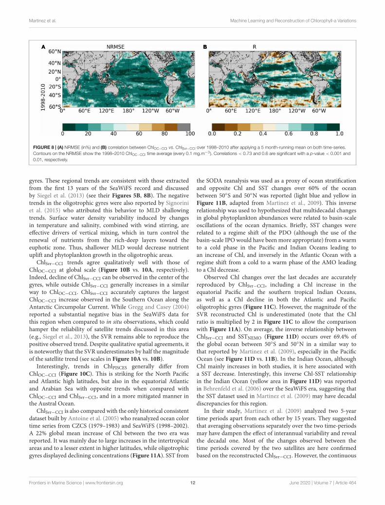
The NRMSE between ChlOC−CCI vs. ChlSvr−CCI is lower than20% over most of the global ocean (Figure 8A). Correlationshigher than 0.9 (p < 0.001) are evident over large subtropicalareas in the Atlantic, Indian and Pacific Oceans as well as in theEquatorial Pacific (Figure 8B). Interestingly, the SVR generallydoes a better job at reconstructing the satellite Chl than themodeled one (Figures 5A,C vs. Figure 8). NRMSE are higherat high latitudes and along the oligotrophic area boundaries,although to a less extent than for ChlPISCES. Because ChlOC−CCI

can only be retrieved under clear sky conditions, gaps in satelliteobservations (especially during wintertime) likely alters the SVRlearning and could explain such a degradation of ChlSvr−CCI asmoving toward high latitudes.

Reconstruction of Satellite ChlInterannual to Decadal Variability andTrendsThe SVR ability to replicate ChlOC−CCI interannual variabilityis now investigated over 1998–2010 (Figure 9). In the PacificOcean, ChlOC−CCI and ChlSvr−CCI 1st EOFs are close (Figure 9Avs. 9B), their PCs are highly correlated (r = 0.89, p < 0.001;Figure 9C), and their percent variance are similar (Table 4). Aspresented in Section “Evaluation of ChlPISCES at global scale,” thismode of Chl variability can be attributed to ENSO, given theirEOFs pattern as well as their PCs highly correlated with the MEI(rOC−CCI/MEI = 0.71 and rSvr−CCI/MEI = 0.91, with p = 0.0015 andp< 0.001, respectively). Interestingly, ChlSvr−CCI EOFs are closerto ChlOC−CCI than ChlPISCES in several areas such as in the north-western Pacific, the south-western Atlantic and the Indian Oceanfrom Madagascar to the western coast of Australia (Figures 9A,Bvs. Figure 3B). Consistently, correlations between ChlOC−CCIand ChlSvr−CCI PCs in the three basins and for the 1st two modesare higher than between ChlOC−CCI and ChlPISCES (Table 4).

ChlOC−CCI linear trends over 1998–2010 exhibit large areasof increase or decrease (red and blue areas in Figure 10A,respectively). Productive regions at high latitudes and alongthe equatorial and upwelling areas generally exhibit positiveChlOC−CCI trends, albeit many underlying regional nuances.Contrastingly, trends are generally negative in the center of the

Frontiers in Marine Science | www.frontiersin.org 11 June 2020 | Volume 7 | Article 464

fmars-07-00464 June 26, 2020 Time: 20:38 # 12

Martinez et al. Machine Learning and Reconstruction of Chlorophyll-a Variations

FIGURE 8 | (A) NRMSE (in%) and (B) correlation between ChlOC−CCI vs. ChlSvr−CCI over 1998–2010 after applying a 5 month-running mean on both time-series.Contours on the NRMSE show the 1998–2010 ChlOC−CCI time average (every 0.1 mg.m−3). Correlations < 0.73 and 0.6 are significant with a p-value < 0.001 and0.01, respectively.

gyres. These regional trends are consistent with those extractedfrom the first 13 years of the SeaWiFS record and discussedby Siegel et al. (2013) (see their Figures 5B, 8B). The negativetrends in the oligotrophic gyres were also reported by Signoriniet al. (2015) who attributed this behavior to MLD shallowingtrends. Surface water density variability induced by changesin temperature and salinity, combined with wind stirring, areeffective drivers of vertical mixing, which in turn control therenewal of nutrients from the rich-deep layers toward theeuphotic zone. Thus, shallower MLD would decrease nutrientuplift and phytoplankton growth in the oligotrophic areas.

ChlSvr−CCI trends agree qualitatively well with those ofChlOC−CCI at global scale (Figure 10B vs. 10A, respectively).Indeed, decline of ChlSvr−CCI can be observed in the center of thegyres, while outside ChlSvr−CCI generally increases in a similarway to ChlOC−CCI. ChlSvr−CCI accurately captures the largestChlOC−CCI increase observed in the Southern Ocean along theAntarctic Circumpolar Current. While Gregg and Casey (2004)reported a substantial negative bias in the SeaWiFS data forthis region when compared to in situ observations, which couldhamper the reliability of satellite trends discussed in this area(e.g., Siegel et al., 2013), the SVR remains able to reproduce thepositive observed trend. Despite qualitative spatial agreements, itis noteworthy that the SVR underestimates by half the magnitudeof the satellite trend (see scales in Figure 10A vs. 10B).

Interestingly, trends in ChlPISCES generally differ fromChlOC−CCI (Figure 10C). This is striking for the North Pacificand Atlantic high latitudes, but also in the equatorial Atlanticand Arabian Sea with opposite trends when compared withChlOC−CCI and ChlSvr−CCI, and in a more mitigated manner inthe Austral Ocean.

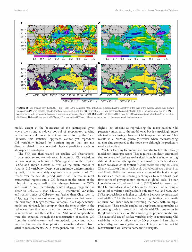
ChlSvr−CCI is also compared with the only historical consistentdataset built by Antoine et al. (2005) who reanalyzed ocean colortime series from CZCS (1979–1983) and SeaWiFS (1998–2002).A 22% global mean increase of Chl between the two era wasreported. It was mainly due to large increases in the intertropicalareas and to a lesser extent in higher latitudes, while oligotrophicgyres displayed declining concentrations (Figure 11A). SST from

the SODA reanalysis was used as a proxy of ocean stratificationand opposite Chl and SST changes over 60% of the oceanbetween 50◦S and 50◦N was reported (light blue and yellow inFigure 11B, adapted from Martinez et al., 2009). This inverserelationship was used to hypothesized that multidecadal changesin global phytoplankton abundances were related to basin-scaleoscillations of the ocean dynamics. Briefly, SST changes wererelated to a regime shift of the PDO (although the use of thebasin-scale IPO would have been more appropriate) from a warmto a cold phase in the Pacific and Indian Oceans leading toan increase of Chl, and inversely in the Atlantic Ocean with aregime shift from a cold to a warm phase of the AMO leadingto a Chl decrease.

Observed Chl changes over the last decades are accuratelyreproduced by ChlSvr−CCI, including a Chl increase in theequatorial Pacific and the southern tropical Indian Oceans,as well as a Chl decline in both the Atlantic and Pacificoligotrophic gyres (Figure 11C). However, the magnitude of theSVR reconstructed Chl is underestimated (note that the Chlratio is multiplied by 2 in Figure 11C to allow the comparisonwith Figure 11A). On average, the inverse relationship betweenChlSvr−CCI and SSTNEMO (Figure 11D) occurs over 69.4% ofthe global ocean between 50◦S and 50◦N in a similar way tothat reported by Martinez et al. (2009), especially in the PacificOcean (see Figure 11D vs. 11B). In the Indian Ocean, althoughChl mainly increases in both studies, it is here associated witha SST decrease. Interestingly, this inverse Chl-SST relationshipin the Indian Ocean (yellow area in Figure 11D) was reportedin Behrenfeld et al. (2006) over the SeaWiFS era, suggesting thatthe SST dataset used in Martinez et al. (2009) may have decadaldiscrepancies for this region.

In their study, Martinez et al. (2009) analyzed two 5-yeartime periods apart from each other by 15 years. They suggestedthat averaging observations separately over the two time-periodsmay have dampen the effect of interannual variability and revealthe decadal one. Most of the changes observed between thetime periods covered by the two satellites are here confirmedbased on the reconstructed ChlSvr−CCI. However, the continuous

Frontiers in Marine Science | www.frontiersin.org 12 June 2020 | Volume 7 | Article 464

fmars-07-00464 June 26, 2020 Time: 20:38 # 13

Martinez et al. Machine Learning and Reconstruction of Chlorophyll-a Variations

FIGURE 9 | First mode of basin-scale EOFs of interannual (A) ChlOC−CCI and (B) ChlSvr−CCI and their associated PCs over 1998–2010 in the (C) Pacific, (D) Indian,and (E) Atlantic Oceans as the black and blue lines, respectively (left y-axis). The climate indices are reported in red on the right y-axis.

TABLE 4 | Percent variance explained by the first two modes of the Empirical Orthogonal Function analysis performed on ChlOC−CCI, ChlSvr−CCI, and ChlPISCES for eachoceanic basin over 1998–2010.

1st mode 2nd mode

% of variance r ChlOC−CCI vs. % of variance r Chl OC−CCI vs.

ChlOC−CCI ChlSvr−CCI ChlPISCES ChlSvr−CCI ChlPISCES ChlOC−CCI ChlSvr−CCI ChlPISCES ChlSvr−CCI ChlPISCES

Pacific 16.6 23.7 21.1 0.89* 0.89* 10.7 12.5 13.6 0.81* 0.52**

Indian 16.9 16.6 17.3 0.57** 0.13 11.8 12.2 15.1 0.48 0.36

Atlantic 14 17.9 19.4 0.85* 0.77* 10.7 9.1 12.5 0.82* 0.59**

The correlation (r) between the PCs of ChlOC−CCI vs. ChlSvr−CCI and between ChlOC−CCI vs. ChlPISCES is also reported with a significant level of *P < 0.001 and **P < 0.02.

Frontiers in Marine Science | www.frontiersin.org 13 June 2020 | Volume 7 | Article 464

fmars-07-00464 June 26, 2020 Time: 20:38 # 14

Martinez et al. Machine Learning and Reconstruction of Chlorophyll-a Variations

FIGURE 10 | Linear trends (in% year −1) calculated over 1998–2010 from the monthly (A) ln(ChlOC−CCI), (B) ln(ChlSvr−CCI), (C) ln(ChlPISCES). Note that the scale isdivided by 2 for ln(ChlSvr−CCI).

30-year time series of ChlSvr−CCI provides new insights on theobserved regime shifts (Figure 12). In the Pacific Ocean, the1st EOF of ChlSvr−CCI (Figure 12A) is close to the Chl spatialpatterns obtained from the CZCS to SeaWiFS era (Figure 11C)and the PC remains highly correlated with the IPO over 1979-2010 (r = 0.94 with p < 0.001, Figure 12B). The Chl increasein the Indian Ocean, north-east of Madagascar toward the westcoast of Australia, between the 1980’s and the 2000’s also appearson the ChlSvr−CCI EOF. These temporal changes might also berelated to the IPO variability (correlation between the IPO indexand ChlSvr−CCI PC = 0.6, p < 0.001; Figure 12C).

In the Atlantic Ocean, CZCS-SeaWiFS Chl and ChlSvr−CCI 1stEOF also share some similarities, including a decrease of Chl inthe subtropical gyres and an increase in the equatorial/tropicalregions. The associated PC (Figure 12D), exhibits a shiftbetween 1979–1983 and 1998–2002 consistently with Figure 2Cof Martinez et al. (2009). In this latter study, this change wasattributed to a regime shift of the AMO. However, the AMOindex is not correlated with the 1st ChlSvr−CCI PC (r = 0.03,p = 0.43) but rather with the 2nd mode (r = 0.43 with p =

0.003, Supplementary Figure 6), likely explaining the spatialdiscrepancies in Figure 11A vs. 11C. Although the detailedanalysis of Chl decadal variability is beyond the scope of thepresent study, these initial findings underscore the importanceof continuous time series at regional/global scales to combinespatial and temporal information’s and properly investigate Chllong-term variability.

SUMMARY AND CONCLUSION

In this paper, we assess the efficiency of a machine learningstatistical approach based on support vector regressionto reconstruct surface Chl from oceanic and atmosphericvariables. We first apply this strategy on a self-consistentglobal dataset gathering physical predictors and Chl datasimulated by a coupled physical-biogeochemical modelsimulation. Our results indicate that this non-linear methodaccurately hindcasts interannual-to-decadal variations ofthe phytoplankton biomass simulated at global scale by the

Frontiers in Marine Science | www.frontiersin.org 14 June 2020 | Volume 7 | Article 464

fmars-07-00464 June 26, 2020 Time: 20:38 # 15

Martinez et al. Machine Learning and Reconstruction of Chlorophyll-a Variations

FIGURE 11 | Chl change from the CZCS (1979–1983) to the SeaWiFS (1998–2002) era, expressed as the logarithm of the ratio of the average values over the twotime periods (A) from satellite Chl adapted from Antoine et al. (2005), (C) from ChlSvr−CCI. Note that this ratio is multiplied by 2 to fit the same color bar as in (A).Maps of areas with concomitant parallel or opposite changes of Chl and SST (B) from Chl satellite and SST from the SODA reanalysis adapted from Martinez et al.(2009) and (D) from ChlSvr−CCI and SSTNEMO. The respective SST zero differences are shown on the maps as a thick black curve.

model, except at the boundaries of the subtropical gyreswhere the strong top-down control of zooplankton grazingin the numerical model is not accounted for by the SVR.Likewise, this statistical approach cannot yet reproduceChl variability induced by nutrient inputs that are notdirectly related to our selected physical predictors, such asatmospheric iron deposit.

The SVR was then trained on satellite Chl observations.It accurately reproduces observed interannual Chl variationsin most regions, including El Niño signature in the tropicalPacific and Indian Oceans as well as the main modes ofAtlantic Chl variability. Despite an amplitude underestimationby half, it also accurately captures spatial patterns of Chltrends over the satellite period, with a Chl increase in mostextratropical regions and a Chl decrease in the center of thesubtropical gyres, as well as their changes between the CZCSand SeaWiFS era. Interestingly, while ChlPISCES magnitude iscloser to ChlOC−CCI than ChlSvr−CCI, interannual variabilityand spatial trends of ChlPISCES are farther than ChlSvr−CCI toChlOC−CCI. Equations representing the processes that governthe evolution of biogeochemical variables in a biogeochemicalmodel are obviously less complex than the ones at play in thereal ocean. We thus anticipated the modeled Chl to be easierto reconstruct than the satellite one. Additional complicationswere also expected through the reconstruction of satellite Chlfrom the model oceanic and atmospheric predictors, whichmay be less realistic than physical parameters derived fromsatellite measurements. As a consequence, the SVR is indeed

slightly less efficient at reproducing the major satellite Chlpatterns compared to the model ones but is surprisingly moreefficient at capturing observed Chl temporal variations. Thisresults in a NRMSE generally weaker when reconstructingsatellite data compared to the model one, although the predictorsused are identical.

Machine learning techniques are powerful tools to statisticallymodel non-linear processes. They require a significant amount ofdata to be trained and are well-suited to analyze remote sensingdata. While several attempts have been made over the last decadeto retrieve oceanic Chl content (Kwiatkowska and Fargion, 2003;Zhan et al., 2003; Camps-Valls et al., 2009; Jouini et al., 2013; Blixand Eltoft, 2018), the present work is one of the first attemptto use such machine learning techniques to reconstruct pasttime series of phytoplankton biomass at global scale. To ourknowledge only Schollaert Uz et al. (2017) tried to reconstructthe Chl multi-decadal variability in the tropical Pacific using acanonical correlation analysis built only from SST and SSH. OurSVR approach leads to higher correlations between reconstructedand satellite Chl in the tropical Pacific, highlighting the strengthof such non-linear machine-learning methods with multiplepredictors. These results emphasize deep learning approaches aspromising tools to reconstruct multidecadal Chl time series inthe global ocean, based on the knowledge of physical conditions.The successful use of surface variables only in reproducing Chlvariability which is influenced by 3D-processes is here clearlynoteworthy, and investigation of variable importance in the Chlreconstruction will deserve some future insights.

Frontiers in Marine Science | www.frontiersin.org 15 June 2020 | Volume 7 | Article 464

fmars-07-00464 June 26, 2020 Time: 20:38 # 16

Martinez et al. Machine Learning and Reconstruction of Chlorophyll-a Variations

FIGURE 12 | (A) 1st mode of basin-scale EOFs of interannual ChlSvr−CCI over 1979–2010 and their corresponding PCs in the (B) Pacific (23.2% of the totalvariance), (C) Indian (15.2% of the total variance), (D) Atlantic (13.5% of the total variance) and (E) Austral Oceans (11.4% of the total variance). IPO is reported inred (right y-axis).

An obvious short-term perspective of the current study isto train a wider range of such statistical models with physicalpredictors from surface satellite observations but also fromobservations within the water column which could be derivedfrom Argo data (i.e., mixed layer and thermocline depth).Including complementary variables such as satellite particulatebackscattering coefficient (as a proxy of the Particulate OrganicCarbon) in the training/reconstruction process should also beconsidered. It would allow to investigate the extent to which

the Chl variability reflects changes in phytoplankton biomassvs. cellular changes in response to light (e.g., Siegel et al.,2005; Westberry et al., 2008; Behrenfeld et al., 2015). Theuse of longitude and latitude as predictors may limit theability to capture long-term trends in the evolution of thebiogeochemical province boundaries, such as the expansion ofthe oligotrophic areas (Polovina et al., 2008; Irwin and Oliver,2009; Staten et al., 2018). Thus, exploring deep learning schemeswhich may not explicitly depend on longitude and latitude,

Frontiers in Marine Science | www.frontiersin.org 16 June 2020 | Volume 7 | Article 464

fmars-07-00464 June 26, 2020 Time: 20:38 # 17

Martinez et al. Machine Learning and Reconstruction of Chlorophyll-a Variations

especially convolutional representations (LeCun et al., 2015), areparticularly appealing. Further efforts need also to be dedicatedto alleviate the issue of the underestimation of the long-termChl trends. For instance, it would be noteworthy to investigatesecular trends such as the 30% Chl decrease reported at globalscale over the last century by Boyce et al. (2010), which remainslargely debated (Mackas, 2011; McQuatters-Gollop et al., 2011;Rykaczewski and Dunne, 2011).

Whatever the methodology used (i.e., numerical models,satellite or in situ observations), they all have both advantagesand drawbacks. In situ observations are considered asground truth (with some errors/uncertainties dependingfor instance on the field measurement protocols), but areheterogeneous in time and space. Satellite Chl data providea spatio-temporal synoptic view but they have their ownmeasurement issues and uncertainties (e.g., radiometricsensors and spectral properties, atmospheric corrections, waterconstituents and their optical properties) and are limitedto 20 years in their record length. Biogeochemical modelsare useful tools to (i) interpolate or extrapolate in timeand space biogeochemical tracers such as Chl and to (ii)investigate complex three-dimensional processes responsiblefor their variations. However, those models also suffer frombiases and are farther from in situ observations than satellitedata. They are also not straightforward to run and requirelarge computing resources. Thus, machine learning statisticalschemes could be seen as a complementary tool to the“interpolate/extrapolate” use of biogeochemical models inproviding a long-term synoptic surface view built fromobservations (being aware of the uncertainties associated withthe variables used in the training schemes). Such methods,applied on observations only, will then provide an independenttool that may either question or enforce conclusions drawnfrom model simulations. Comparison between both methodsand observations will help to improve biogeochemical modelswith acute quantification of model biases and identificationof the most meaningful predictors that may point to missingprocesses in biogeochemical models. As a conclusion, machinelearning is a versatile tool that, associated with biogeochemicalmodels and observations, may greatly enhance our view of globalbiogeochemistry.

DATA AVAILABILITY STATEMENT

Publicly available datasets were analyzed in this study. Climateindices can be found at: www.esrl.noaa.gov/psd and Chl satelliteat: http://www.esa-oceancolour-cci.org/. The model predictorscan be found at: http://data.umr-lops.fr/pub/AFCM85/HISTORICAL_OCEAN/ and http://data.umr-lops.fr/pub/AFCM85/HISTORICAL_ATM/DFS5_1979-2012/. ReconstructedChl can be found at: http://data.umr-lops.fr/pub/DeepLearning/PhytoDev_SVR.

AUTHOR CONTRIBUTIONS

EM led the project, analyzed the results, and wrote the first draftof the manuscript. TG provided the physical model outputs. TGand ML provided support in the analysis and the writing of themanuscript. CF processed the machine learning approach withsupport from RS. RF provided the feedbacks on the statisticalapproach. All the authors contributed to the development ofthe manuscript and provided the feedbacks throughout its manystages of preparation.

FUNDING

This work was supported by CNES under contract n◦160515/00within the framework of the PhytoDev project.

ACKNOWLEDGMENTS

We thank the two reviewers who helped to improvethis manuscript. C. Berthin is also thanked forproviding Figure 11.

SUPPLEMENTARY MATERIAL

The Supplementary Material for this article can be foundonline at: https://www.frontiersin.org/articles/10.3389/fmars.2020.00464/full#supplementary-material

REFERENCESAguilar-Martinez, S., and Hsieh, W. W. (2009). Forecasts of tropical pacific sea

surface temperatures by neural networks and support vector regression. Int. J.Oceanog. 2009:167239. doi: 10.1155/2009/167239

Antoine, D., Morel, A., Gordon, H. R., Banzon, V. F., and Evans, R. H. (2005).Bridging ocean color observations of the 1980s and 2000s in search of long-termtrends. J. Geophys. Res. Oceans 110:C06009.

Aumont, O., and Bopp, L. (2006). Globalizing results from ocean in situiron fertilization studies. Glob. Biogeochem. Cycles 20:GB2017. doi: 10.1029/2005GB002591

Aumont, O., Ethé, C., Tagliabue, A., Bopp, L., and Gehlen, M. (2015). PISCES-v2: an ocean biogeochemical model for carbon and ecosystem studies. Geosci.Model Dev. 8, 2465–2513. doi: 10.5194/gmd-8-2465-2015

Ayata, S. D., Lévy, M., Aumont, O., Sciandra, A., Sainte-Marie, J., Tagliabue, A.,et al. (2013). Phytoplankton growth formulation in marine ecosystem models:

should we take into account photoacclimation and variable stoichiometry inoligotrophic areas? J. Mar. Syst. 125, 29–40. doi: 10.1016/j.jmarsys.2012.12.010

Banse, K., and English, D. C. (2000). Geographical differences in seasonality ofCZCS-derived phytoplankton pigment in the Arabian Sea for 1978-1986. DeepSea Res. II Top. Stud. Oceanogr. 47, 1623–1677. doi: 10.1016/s0967-0645(99)00157-5

Beaulieu, C., Henson, S. A., Sarmiento, J. L., Dunne, J. P., Doney, S. C.,Rykaczewski, R. R., et al. (2013). Factors challenging our ability to detect long-term trends in ocean chlorophyll. Biogeosciences 10, 2711–2724. doi: 10.5194/bg-10-2711-2013

Behrenfeld, M. J., O’Malley, R. T., Boss, E. S., Westberry, T. K., Graff, J. R.,Halsey, K. H., et al. (2015). Revaluating ocean warming impacts on globalphytoplankton. Nat. Clim. Chang. 6, 323–330. doi: 10.1038/nclimate2838

Behrenfeld, M. J., O’Malley, R. T., Siegel, D. A., McClain, C. R., Sarmiento, J. L.,Feldman, G. C., et al. (2006). Climate-driven trends in contemporary oceanproductivity. Nature 444, 752–755. doi: 10.1038/nature05317

Frontiers in Marine Science | www.frontiersin.org 17 June 2020 | Volume 7 | Article 464

fmars-07-00464 June 26, 2020 Time: 20:38 # 18

Martinez et al. Machine Learning and Reconstruction of Chlorophyll-a Variations

Behrenfeld, M. J., Randerson, J. T., McClain, C. R., Feldman, G. C., Los, S. O.,Tucker, C. J., et al. (2001). Biospheric primary production during an ENSOtransition. Science 291, 2594–2597. doi: 10.1126/science.1055071

Belo Couto, A., Brotas, V., Mélin, F., Groom, S., and Sathyendranath, S. (2016).Inter-comparison of OC-CCI chlorophyll-a estimates with precursor data sets.Int. J. Remote Sens. 37, 4337–4355. doi: 10.1080/01431161.2016.1209313

Blix, K., and Eltoft, T. (2018). Machine learning automatic model selectionalgorithm for oceanic chlorophyll-a content retrieval. Remote Sens. 10:775.doi: 10.3390/rs10050775

Bopp, L., Aumont, O., Cadule, P., Alvain, S., and Gehlen, M. (2005). Responseof diatoms distribution to global warming and potential implications: a globalmodel study. Geophys. Res. Lett. 32:L19606.

Boyce, D. G., Lewis, M. R., and Worm, B. (2010). Global phytoplankton declineover the past century. Nature 466, 591–596. doi: 10.1038/nature09268

Campbell, J. W., and Aarup, T. (1992). New production in the North Atlanticderived from seasonal patterns of surface chlorophyll. Deep Sea Res. A 39,1669–1694. doi: 10.1016/0198-0149(92)90023-m

Camps-Valls, G., Muñoz-Marí, J. L., Gómez-Chova, K. R., and Calpe-Maravilla, J.(2009). Biophysical parameter estimation with a semisupervised support vectormachine. IEEE Geosci. Remote Sens. Lett. 6, 248–252. doi: 10.1109/lgrs.2008.2009077

Chavez, F. P., Messié, M., and Pennington, J. T. (2011). Marine primary productionin relation to climate variability and change. Annu. Rev. Mar. Sci. 3, 227–260.doi: 10.1146/annurev.marine.010908.163917

Chavez, F. P., Strutton, P. G., Friederich, G. E., Feely, R. A., Feldman, G. C., Foley,D. G., et al. (1999). Biological and chemical response of the equatorial PacificOcean to the 1997-98 El Niño. Science 286, 2126–2131. doi: 10.1126/science.286.5447.2126

Currie, J. C., Lengaigne, M., Vialard, J., Kaplan, D., Aumont, O., Naqvi, S. W. A.,et al. (2013). Indian Ocean dipole and El Nino/southern oscillation impactson regional chlorophyll anomalies in the Indian Ocean. Biogeosciences 10,6677–6698. doi: 10.5194/bg-10-6677-2013

Dandonneau, Y., Deschamps, P. Y., Nicolas, J. M., Loisel, H., Blanchot, J., Montel,Y., et al. (2004). Seasonal and interannual variability of ocean color andcomposition of phytoplankton communities in the North Atlantic, equatorialPacific and South Pacific. Deep Sea Res. II Top. Stud. Oceanogr. 51, 303–318.doi: 10.1016/j.dsr2.2003.07.018

Descloux, E., Mangeas, M., Menkes, C. E., Lengaigne, M., Leroy, A., Tehei, T.,et al. (2012). Climate-based models for understanding and forecasting dengueepidemics. PLoS Negl. Trop. Dis. 6:e1470. doi: 10.1371/journal.pntd.0001470

Dierssen, H. M., and Smith, R. C. (2000). Bio-optical properties and remote sensingocean color algorithms for Antarctic Peninsula waters. J. Geophys. Res. Oceans105, 26301–26312. doi: 10.1029/1999JC000296

D’Ortenzio, F., Antoine, D., Martinez, E., and Ribera d’Alcalà, M. (2012).Phenological changes of oceanic phytoplankton in the 1980s and 2000s asrevealed by ocean-color remote-sensing observations. Glob. Biogeochem. Cycles26:GB4003.

Dussin, R., Barnier, B., Brodeau, L., and Molines, J. M. (2014). The Making ofDrakkar Forcing Set DFS5, DRAKKAR/MyOcean Report 01-04-16. Grenoble:LGGE.

Dutheil, C., Aumont, O., Gorguès, T., Lorrain, A., Bonnet, S., Rodier, M., et al.(2018). Modelling N2 fixation related to Trichodesmium sp.: driving processesand impacts on primary production in the tropical Pacific Ocean. Biogeosciences15, 4333–4352. doi: 10.5194/bg-15-4333-2018

Dutkiewicz, S., Follows, M., Marshall, J., and Gregg, W. W. (2001). Interannualvariability of phytoplankton abundances in the North Atlantic. Deep Sea Res. IITop. Stud. Oceanogr. 48, 2323–2344. doi: 10.1016/s0967-0645(00)00178-8

Dutkiewicz, S., Follows, M. J., and Parekh, P. (2005). Interactions of the iron andphosphorus cycles: a three-dimensional model study. Glob. Biogeochem. Cycles19:GB1021. doi: 10.1029/2004GB002342

Elbisy, M. S. (2015). Sea wave parameters prediction by support vector machineusing a genetic algorithm. J. Coastal Res. 31, 892–899. doi: 10.2112/jcoastres-d-13-00087.1

Emery, W., and Thomson, R. (1997). Data Analysis in Physical Oceanography.(New York, NY: Pergamon), 634

Enfield, D. B., Mestas Nunez, A. M., and Trimble, P. J. (2001). The Atlanticmultidecadal oscillation and its relation to rainfall and river flows in thecontinental U.S. Geophys. Res. Lett. 28, 2077–2080. doi: 10.1029/2000gl012745

Feng, J., Durant, J. M., Stige, L. C., Hessen, D. O., Hjermann, D. Ø., Zhu, L., et al.(2015). Contrasting correlation patterns between environmental factors andchlorophyll levels in the global ocean. Glob. Biogeochem. Cycles 29, 2095–2107.doi: 10.1002/2015GB005216

Garcia, H. E., Locarnini, R. A., Boyer, T. P., and Antonov, J. I. (2006). “World OceanAtlas 2005, Volume 4: Nutrients (phosphate, nitrate, silicate),” in NOAA AtlasNESDIS 64, ed. S. Levitus (Washington, DC: U.S. Government Printing Office),396.

Gehlen, M., Bopp, L., Emprin, N., Aumont, O., Heinze, C., and Ragueneau, O.(2006). Reconciling surface ocean productivity, export fluxes and sedimentcomposition in a global biogeochemical ocean model. Biogeosciences 3, 521–537. doi: 10.5194/bg-3-521-2006

Gnanadesikan, A., Slater, R. J., Gruber, N., and Sarmiento, J. L. (2002). Oceanicvertical exchange and new production: a comparison between models andobservations. Deep Sea Res. II Top. Stud. Oceanogr. 49, 363–401. doi: 10.1016/s0967-0645(01)00107-2

Gregg, W. W., and Casey, N. W. (2004). Global and regional evaluation of theSeaWiFS chlorophyll data set. Remote Sens. Environ. 93, 463–479. doi: 10.1016/j.rse.2003.12.012

Gregg, W. W., and Conkright, M. E. (2002). Decadal changes in global oceanchlorophyll. Geophys. Res. Lett. 29, 20–21.

Gregg, W. W., and Rousseaux, C. S. (2014). Decadal trends in global pelagic oceanchlorophyll: a new assessment integrating multiple satellites, in situ data, andmodels. J. Geophys. Res. Oceans 119, 5921–5933. doi: 10.1002/2014jc010158

Henson, S. A., Beaulieu, C., and Lampitt, R. (2016). Observing climate changetrends in ocean biogeochemistry: when and where. Glob. Change Biol. 22,1561–1571. doi: 10.1111/gcb.13152

Henson, S. A., Dunne, J. P., and Sarmiento, J. L. (2009a). Decadal variability inNorth Atlantic phytoplankton blooms. J. Geophys. Res. Oceans 114:C04013.

Henson, S. A., Raitsos, D., Dunne, J. P., and McQuatters-Gollop, A. (2009b).Decadal variability in biogeochemical models: comparison with a 50-year oceancolour dataset. Geophys. Res. Lett. 36:L21061.

Hood, R. R., Kohler, K. E., McCreary, J. P., and Smith, S. L. (2003). A four-dimensional validation of a coupled physical-biological model of the ArabianSea. Deep Sea Res. II Top. Stud. Oceanogr. 50, 2917–2945. doi: 10.1016/j.dsr2.2003.07.004

Hovis, W. A., Clark, D. K., Anderson, F., Austin, R. W., Wilson, W. H., Baker,E. T., et al. (1980). Nimbus-7 Coastal Zone Color Scanner: system descriptionand initial imagery. Science 210, 60–63. doi: 10.1126/science.210.4465.60

Hu, S., Liu, H., Zhao, W., Shi, T., Hu, Z., Li, Q., et al. (2018). Comparison ofmachine learning techniques in inferring phytoplankton size classes. RemoteSens. 10:191. doi: 10.3390/rs10030191

Huang, B., Thorne, P. W., Banzon, V. F., Boyer, T., Chepurin, G., Lawrimore,J. H., et al. (2017). Extended reconstructed sea surface temperature, version5 (ERSSTv5): upgrades, validations, and intercomparisons. J. Clim. 30, 8179–8205. doi: 10.1175/jcli-d-16-0836.1

Irwin, A. J., and Oliver, M. J. (2009). Are ocean deserts getting larger? Geophys. Res.Lett. 36:L18609. doi: 10.1029/2009GL039883

Jickells, T. D., An, Z. S., Andersen, K. K., Baker, A. R., Berga-metti, G.,Brooks, N., et al. (2005). Global iron connections between desert dust, oceanbiogeochemistry, and climate. Nature 308, 67–71. doi: 10.1126/science.1105959

Jouini, M., Lévy, M., Crépon, M., and Thiria, S. (2013). Reconstruction of satellitechlorophyll images under heavy cloud coverage using a neural classificationmethod. Remote Sens. Environ. 131, 232–246. doi: 10.1016/j.rse.2012.11.025

Kahru, M., Gille, S. T., Murtugudde, R., Strutton, P. G., Manzano-Sarabia,M., Wang, H., et al. (2010). Global correlations between winds and oceanchlorophyll. J. Geophys. Res. Oceans 115:C12040. doi: 10.1029/2010JC006500

Kahru, M., and Mitchell, B. G. (2010). Blending of ocean colour algorithmsapplied to the Southern Ocean. Remote Sens. Lett. 1, 119–124. doi: 10.1080/01431160903547940

Keerthi, M. G., Lengaigne, M., Levy, M., Vialard, J., and de Boyer Montegut, C.(2017). Physical control of interannual variations of the winter chlorophyllbloom in the northern Arabian Sea. Biogeosciences 14, 3615–3632. doi: 10.5194/bg-14-3615-2017

Kim, Y. H., Im, J., Ha, H. K., Choi, J. K., and Ha, S. (2014). Machinelearning approaches to coastal water quality monitoring using GOCIsatellite data. GISci. Remote Sens. 51, 158–174. doi: 10.1080/15481603.2014.900983

Frontiers in Marine Science | www.frontiersin.org 18 June 2020 | Volume 7 | Article 464

fmars-07-00464 June 26, 2020 Time: 20:38 # 19

Martinez et al. Machine Learning and Reconstruction of Chlorophyll-a Variations

Kwiatkowska, E. J., and Fargion, G. S. (2003). Application of machine-learningtechniques toward the creation of a consistent and calibrated global chlorophyllconcentration baseline dataset using remotely sensed ocean color data.IEEE Trans. Geosci. Remote Sens. 41, 2844–2860. doi: 10.1109/tgrs.2003.818016

Laufkötter, C., Vogt, M., Gruber, N., Aita-Noguchi, M., Aumont, O., Bopp, L., et al.(2015). Drivers and uncertainties of future global marine primary productionin marine ecosystem models. Biogeosciences 12, 6955–6984. doi: 10.5194/bg-12-6955-2015

Launois, T., Belviso, S., Bopp, L., Fichot, C. G., and Peylin, P. (2015). Anew model for the global biogeochemical cycle of carbonyl sulfide–Part 1:assessment of direct marine emissions with an oceanic general circulation andbiogeochemistry model. Atmos. Chem. Phys. 15, 2295–2312. doi: 10.5194/acp-15-2295-2015

Laws, E. A., and Bannister, T. T. (1980). Nutrient-and light-limited growthof Thalassiosira fluviatilis in continuous culture, with implications forphytoplankton growth in the ocean. Limnol. Oceanogr. 25, 457–473. doi: 10.4319/lo.1980.25.3.0457

LeCun, Y., Bengio, Y., and Hinton, G. (2015). Deep learning. Nature 521, 436–444.doi: 10.1038/nature14539

Lengaigne, M., Menkes, C., Aumont, O., Gorgues, T., Bopp, L., André, J. -M.,et al. (2007). Influence of the oceanic biology on the tropical Pacific climatein a Coupled General Circulation Model. Clim. Dyn. 28, 503–516. doi: 10.1007/s00382-006-0200-2

Lewandowska, A. M., Hillebrand, H., Lengfellner, K., and Sommer,U. (2014). Temperature effects on phytoplankton diversity—Thezooplankton link. J. Sea Res. 85, 359–364. doi: 10.1016/j.seares.2013.07.003

Longhurst, A., Sathyendranath, S., Platt, T., and Caverhill, C. (1995).An estimate of global primary production in the ocean from satelliteradiometer data. J. Plankton Res. 17, 1245–1271. doi: 10.1093/plankt/17.6.1245

Mackas, D. L. (2011). Does blending of chlorophyll data bias temporal trend?Nature 472, E4–E5.

Madec, G. (2008). NEMOReference Manual, Ocean Dynamics Component: NEMO-OPA. Preliminary version. Note du Pole de Modélisation. Jussieu: InstitutPierre-Simon Laplace (IPSL), 1288–1161.

Mantua, N. J., Hare, S. R., Zhang, Y., Wallace, J. M., and Francis, R. C.(1997). A pacific interdecadal climate oscillation with impacts on salmonproduction. Bull. Am. Meteorol. Soc. 78, 1069–1079. doi: 10.1175/1520-0477(1997)078<1069:apicow>2.0.co;2

Martinez, E., Antoine, D., D’Ortenzio, F., and de Boyer Montégut, C. (2011).Phytoplankton spring and fall blooms in the North Atlantic in the 1980s and2000s. J. Geophys. Res. Oceans 116:C11029.

Martinez, E., Antoine, D., D’Ortenzio, F., and Gentili, B. (2009). Climate-drivenbasin-scale decadal oscillations of oceanic phytoplankton. Science 36, 1253–1256. doi: 10.1126/science.1177012

Martinez, E., Raitsos, D., and Antoine, D. (2016). Warmer, deeperand greener mixed layers in the north Atlantic subpolar gyre overthe last 50 years. Glob. Change Biol. 22, 604–612. doi: 10.1111/gcb.13100

McClain, C. R., Christian, J. R., Signorini, S. R., Lewis, M. R., Asanuma, I., Turk,D., et al. (2002). Satellite ocean-color observations of the tropical Pacific Ocean.Deep Sea Res. II Top. Stud. Oceanogr. 49, 2533–2560. doi: 10.1016/s0967-0645(02)00047-4

McClain, C. R., Feldman, G., and Hooker, S. (2004). An overview of the SeaWiFSproject and strategies for producing a climate research quality global oceanbio-optical time series. Deep Sea Res. II Top. Stud. Oceanogr. 51, 5–42. doi:10.1016/j.dsr2.2003.11.001

McQuatters-Gollop, A., Reid, P. C., Edwards, M., Burkill, P. H., Castellani, C.,Batten, S., et al. (2011). Is there a decline in marine phytoplankton? Nature 472,E6–E7.

Messié, M., and Chavez, F. P. (2012). A global analysis of ENSO synchrony:the oceans’ biological response to physical forcing. J. Geophys. Res. Oceans,117:C09001. doi: 10.1029/2012JC007938

Messié, M., and Chavez, F. P. (2015). Seasonal regulation of primary production ineastern boundary upwelling systems. Prog. Oceanogr. 134, 1–18. doi: 10.1016/j.pocean.2014.10.011

Morel, A., and Gentili, B. (2009). The dissolved yellow substance and the shades ofblue in the Mediterranean Sea. Biogeosciences 6, 2625–2636. doi: 10.5194/bg-6-2625-2009

Murtugudde, R. G., Signorini, S. R., Christian, J. R., Busalacchi, A. J., McClain,C. R., and Picaut, J. (1999). Ocean color variability of the tropical Indo-Pacificbasin observed by SeaWiFS during 1997– 1998. J. Geophys. Res. Oceans 104,18351–18366. doi: 10.1029/1999jc900135

Neetu, S., Lengaigne, M., Mangeas, M., Vialard, J., Leloup, J., Menkes C., et al.(2020). Quantifying the benefits of non-linear methods for global statisticalhindcasts of tropical cyclones intensity. Mon. Weather Rev. 35, 807–820. doi:10.1175/WAF-D-19-0163.1

Nidheesh, A. G., Lengaigne, M., Vialard, J., Izumo, T., Unnikrishnan, A. S.,Meyssignac, B., et al. (2017). Robustness of observation-based decadal sea levelvariability in the Indo-Pacific Ocean. Geophys. Res. Lett 44, 7391–7400. doi:10.1002/2017gl073955

Parvathi, V., Suresh, I., Lengaigne, M., Ethé, C., Vialard, J., Levy, M., et al. (2017).Positive Indian Ocean Dipole events prevent anoxia along the west coast ofIndia. Biogeosciences 14, 1541–1559. doi: 10.5194/bg-14-1541-2017

Patara, L., Visbeck, M., Masina, S., Krahmann, G., and Vichi, M. (2011). Marinebiogeochemical responses to the North Atlantic Oscillation in a coupled climatemodel. J. Geophys. Res. Oceans 116:C07023.

Polovina, J. J., Howell, E. A., and Abecassis, M. (2008). Ocean’s leastproductive waters are expanding. Geophys. Res. Lett. 35:L03618. doi: 10.1029/2007GL031745

Radenac, M. H., Léger, F., Singh, A., and Delcroix, T. (2012). Sea surfacechlorophyll signature in the tropical Pacific during eastern and central PacificENSO events. J. Geophys. Res. Oceans 117:C04007.

Radenac, M. H., Messié, M., Léger, F., and Bosc, C. (2013). A very oligotrophic zoneobserved from space in the equatorial Pacific warm pool. Remote Sens. Environ.134, 224–233. doi: 10.1016/j.rse.2013.03.007

Resplandy, L., Lévy, M., Madec, G., Pous, S., Aumont, O., and Kumar, D. (2011).Contribution of mesoscale processes to nutrient budgets in the Arabian Sea.J. Geophys. Res. Oceans 116:C04007.

Rykaczewski, R. R., and Dunne, J. P. (2011). A measured look at ocean chlorophylltrends. Nature 472, E5–E6.

Saji, N. H., Goswami, B. N., Vinayachandran, P. N., and Yamagata, T. (1999). Adipole mode in the tropical Indian Ocean. Nature 401, 360–363. doi: 10.1038/43854

Sakamoto, T., Gitelson, A. A., Wardlow, B. D., Verma, S. B., and Suyker, A. E.(2011). Estimating daily gross primary production of maize based only onMODIS WDRVI and shortwave radiation data. Remote Sens. Environ. 115,3091–3101. doi: 10.1016/j.rse.2011.06.015

Sauzède, R., Claustre, H., Jamet, C., Uitz, J., Ras, J., Mignot, A., et al.(2015). Retrieving the vertical distribution of chlorophyll a concentration andphytoplankton community composition from in situ fluorescence profiles: Amethod based on a neural network with potential for global-scale applications.J. Geophys. Res. Oceans 120, 451–470. doi: 10.1002/2014JC010355

Schneider, B., Bopp, L., Gehlen, M., Segschneider, J., Frölicher, T. L., Cadule,P., et al. (2008). Climate-induced interannual variability of marine primaryand export production in three global coupled climate carbon cycle models.Biogeosciences 5, 597–614. doi: 10.5194/bg-5-597-2008

Schollaert Uz, S., Busalacchi, A. J., Smith, T. M., Evans, M. N., Brown, C. W.,Hackert, E. C., et al. (2017). Interannual and decadal variability in tropicalpacific chlorophyll from a statistical reconstruction: 1958–2008. J. Clim. 30,7293–7315. doi: 10.1175/JCLI-D-16-0202.1

Séférian, R., Bopp, L., Gehlen, M., Orr, J. C., Ethé, C., Cadule, P., et al.(2013). Skill assessment of three earth system models with common marinebiogeochemistry. Clim. Dyn. 40, 2549–2573. doi: 10.1007/s00382-012-1362-8

Siegel, D. A., Behrenfeld, M. J., Maritorena, S., McClain, C. R., Antoine, D., Bailey,S. W., et al. (2013). Regional to global assessments of phytoplankton dynamicsfrom the SeaWiFS mission. Remote Sens. Environ. 135, 77–91. doi: 10.1016/j.rse.2013.03.025

Siegel, D. A., Maritorena, S., Nelson, N. B., and Behrenfeld, M. J. (2005).Independence and interdependencies among global ocean color properties:reassessing the bio-optical assumption. J. Geophys. Res. Oceans 110:C07011.

Signorini, S. R., Franz, B. A., and McClain, C. R. (2015). Chlorophyll variability inthe oligotrophic gyres: mechanisms, seasonality and trends. Front. Mar. Sci. 2:1.doi: 10.3389/fmars.2015.00001

Frontiers in Marine Science | www.frontiersin.org 19 June 2020 | Volume 7 | Article 464

fmars-07-00464 June 26, 2020 Time: 20:38 # 20

Martinez et al. Machine Learning and Reconstruction of Chlorophyll-a Variations

Signorini, S. R., and McClain, C. R. (2012). Subtropical gyre variability as seen fromsatellites. Remote Sens. Lett. 3, 471–479. doi: 10.1080/01431161.2011.625053

Smith, T. M., Arkin, P. A., Ren, L., and Shen, S. S. (2012). Improved reconstructionof global precipitation since 1900. J. Atmos. Ocean Technol. 29, 1505–1517.doi: 10.1175/jtech-d-12-00001.1

Staten, P. W., Lu, J., Grise, K. M., Davis, S. M., and Birner, T. (2018). Re-examiningtropical expansion. Nat. Clim. Change 8, 768–775. doi: 10.1038/s41558-018-0246-2

Steinacher, M., Joos, F., Frölicher, T. L., Bopp, L., Cadule, P., Cocco, V., et al. (2010).Projected 21st century decrease in marine productivity: a multi-model analysis.Biogeosciences 7, 979–1005. doi: 10.5194/bg-7-979-2010

Storm, T., Boettcher, M., Grant, M., Zühlke, M., Fomferra, N., Jackson, T., et al.(2013). Product User Guide, Ocean Colour Climate Change Initiative. Availableonline at: www.esa-oceancolour-cci.org/?q=webfm_send/317

Tagliabue, A., Bopp, L., Dutay, J. C., Bowie, A. R., Chever, F., Jean-Baptiste, P., et al.(2010). Hydrothermal contribution to the oceanic dissolved iron inventory.Nat.Geosci. 3, 252–256. doi: 10.1038/ngeo818

Tang, W., Li, Z., and Cassar, N. (2019). Machine learning estimates of globalmarine nitrogen fixation. J. Geophys. Res. Biogeosci. 124, 717–730. doi: 10.1029/2018jg004828

Thomas, A. C., Strub, P. T., Weatherbee, R. A., and James, C. (2012). Satelliteviews of Pacific chlorophyll variability: Comparisons to physical variability,local versus nonlocal influences and links to climate indices. DeepSea Res. IITop. Stud. Oceanogr. 77, 99–116. doi: 10.1016/j.dsr2.2012.04.008

Vantrepotte, V., and Mélin, F. (2009). Temporal variability of 10-year globalSeaWiFS time-series of phytoplankton chlorophyll a concentration. ICES J.Mar. Sci. 66, 1547–1556. doi: 10.1093/icesjms/fsp107

Vantrepotte, V., and Mélin, F. (2011). Inter-annual variations in the SeaWiFS globalchlorophyll a concentration (1997–2007). Deep Sea Res. Part I Oceanogr. Res.Pap. 58, 429–441. doi: 10.1016/j.dsr.2011.02.003

Vapnik, V. (1998). “The support vector method of function estimation,” inNonlinear Modeling, eds J. Suykens, and J. Vandewalle (Boston, MA: KluwerAcademic Publishers), 55–85. doi: 10.1007/978-1-4615-5703-6_3

Vapnik, V. (2000). “Statistics for engineering and information science,” in TheNature of Statistical Learning Theory, eds M. J. Jordan, J. F. Lawless, S. L.Lauritzen, and V. Nair (New York, NY: Springer).

Vapnik, V. N. (1995). The Nature of Statistical Learning Theory. New York, NY:Springer Verlag.

Westberry, T., Behrenfeld, M. J., Siegel, D. A., and Boss, E. (2008). Carbon-basedprimary productivity modeling with vertically resolved photoacclimation. Glob.Biogeochem. Cycles 22:GB2024.

Wiggert, J. D., Murtugudde, R. G., and Christian, J. R. (2006). Annual ecosystemvariability in the tropical Indian Ocean: Results of a coupled bio-physical oceangeneral circulation model. Deep Sea Res. II Top. Stud. Oceanogr. 53, 644–676.doi: 10.1016/j.dsr2.2006.01.027

Wiggert, J. D., Vialard, J., and Behrenfeld, M. J. (2009). “Basin wide modificationof dynamical and biogeochemical processes by the positive phase of theIndian Ocean Dipole during the SeaWiFS era,” in Indian Ocean BiogeochemicalProcesses and Ecological Variability, Vol. 185, eds J. D. Wiggert, R. R. Hood,S. Wajih, A. Naqvi, K. H. Brink, and S. L. Smith (Washington, DC: AGU),350.

Wilson, C., and Adamec, D. (2001). Correlations between surface chlorophyll andsea surface height in the tropical Pacific during the 1997-1999 El Nino-Southernevent. J. Geophys. Res. Oceans 106, 31175–31188. doi: 10.1029/2000jc000724

Wilson, C., and Adamec, D. (2002). A global view of bio-physical coupling fromSeaWiFS and TOPEX satellite data, 1997–2001. Geophys. Res. Lett. 29:1257.doi: 10.1029/2001GL014063

Wilson, C., and Coles, V. J. (2005). Global climatological relationships betweensatellite biological and physical observations and upper ocean properties.J. Geophys. Res. Oceans 110:C10001. doi: 10.1029/2004JC002724

Yoder, J. A., and Kennelly, M. A. (2003). Seasonal and ENSO variability inglobal ocean phytoplankton chlorophyll derived from 4 years of SeaWiFSmeasurements. Glob. Biogeochem. Cycles 17:1112. doi: 10.1029/2002GB001942

Yoo, S., and Son, S. -H. (1998). Seasonal patterns of phytoplankton biomass changein the Northwestern Pacific Marginal Seas observed by CZCS. Ocean Res. 20,29–42.

Zhan, H., Shi, P., and Chen, C. (2003). Retrieval of oceanic chlorophyllconcentration using support vector machines. IEEE Trans. Geosci. Remote Sens.41, 2947–2951. doi: 10.1109/tgrs.2003.819870

Conflict of Interest: The authors declare that the research was conducted in theabsence of any commercial or financial relationships that could be construed as apotential conflict of interest.

Copyright © 2020 Martinez, Gorgues, Lengaigne, Fontana, Sauzède, Menkes, Uitz,Di Lorenzo and Fablet. This is an open-access article distributed under the termsof the Creative Commons Attribution License (CC BY). The use, distribution orreproduction in other forums is permitted, provided the original author(s) and thecopyright owner(s) are credited and that the original publication in this journalis cited, in accordance with accepted academic practice. No use, distribution orreproduction is permitted which does not comply with these terms.

Frontiers in Marine Science | www.frontiersin.org 20 June 2020 | Volume 7 | Article 464

CORRECTIONpublished: 26 November 2020

doi: 10.3389/fmars.2020.618249

Frontiers in Marine Science | www.frontiersin.org 1 November 2020 | Volume 7 | Article 618249

Edited and reviewed by:

Juliet Hermes,

South African Environmental

Observation Network (SAEON),

South Africa

*Correspondence:

Elodie Martinez

elodie.martinez@ird.fr

†Present address:

Matthieu Lengaigne,

MARBEC, University of Montpellier,

CNRS, IFREMER, IRD, Sete, France

Raphaëlle Sauzède,

CNRS-INSU, Institut de la Mer de

Villefranche, Sorbonne Universités,

Villefranche-sur-Mer, France

Specialty section:

This article was submitted to

Ocean Observation,

a section of the journal

Frontiers in Marine Science

Received: 16 October 2020

Accepted: 05 November 2020

Published: 26 November 2020

Citation:

Martinez E, Gorgues T, Lengaigne M,

Fontana C, Sauzède R, Menkes C,

Uitz J, Di Lorenzo E and Fablet R

(2020) Corrigendum: Reconstructing

Global Chlorophyll-a Variations Using

a Non-linear Statistical Approach.

Front. Mar. Sci. 7:618249.

doi: 10.3389/fmars.2020.618249

Corrigendum: Reconstructing GlobalChlorophyll-a Variations Using aNon-linear Statistical ApproachElodie Martinez 1,2*, Thomas Gorgues 1, Matthieu Lengaigne 3†, Clement Fontana 2,

Raphaëlle Sauzède 2†, Christophe Menkes 4, Julia Uitz 5, Emanuele Di Lorenzo 6 and

Ronan Fablet 7

1 LOPS, IUEM, IRD, Ifremer, CNRS, Univ. Brest, Brest, France, 2 EIO, IRD, Ifremer, UPF and ILM, Tahiti, French Polynesia,3 LOCEAN-IPSL, Sorbonne Universités/UPMC-CNRS-IRD-MNHN, Paris, France, 4 ENTROPIE, IRD, Univ. de la Réunion,

CNRS, Univ. de la Nouvelle Calédonie, Ifremer, Noumea, New Caledonia, 5 Laboratoire d’Océanographie de Villefranche,

CNRS and Sorbonne Université, Villefranche-sur-Mer, France, 6Georgia Institute of Technology, Atlanta, GA, United States,7 IMT Atlantique, Lab-STICC, UMR CNRS 6285, Brest, France

Keywords: machine learning, phytoplankton variability, satellite ocean color, decadal variability, global scale

A Corrigendum on

Reconstructing Global Chlorophyll-a Variations Using a Non-linear Statistical Approach

byMartinez, E., Gorgues, T., Lengaigne, M., Fontana, C., Sauzède, R., Menkes, C., et al. (2020). Front.Mar. Sci. 7:464. doi: 10.3389/fmars.2020.00464

In the original article, there was a mistake in the labeling of the Figures 11B and Figures 11D

color bar as published. The SST-Chl opposite relationship labels below the color bar were invertedbetween the green and yellow sections. The corrected Figure 11 appears below.

The authors apologize for this error and state that this does not change the scientific conclusionsof the article in any way. The original article has been updated.

REFERENCES

Antoine, D., Morel, A., Gordon, H. R., Banzon, V. F., and Evans, R. H. (2005). Bridging ocean color observations of the 1980s

and 2000s in search of long-term trends. J. Geophys. Res. Oceans 110:C06009.

Martinez, E., Antoine, D., D’Ortenzio, F., and Gentili, B. (2009). Climate-driven basin-scale decadal oscillations of oceanic

phytoplankton. Science 36, 1253–1256. doi: 10.1126/science.1177012

Copyright © 2020 Martinez, Gorgues, Lengaigne, Fontana, Sauzède, Menkes, Uitz, Di Lorenzo and Fablet. This is an open-access

article distributed under the terms of the Creative Commons Attribution License (CC BY). The use, distribution or reproduction

in other forums is permitted, provided the original author(s) and the copyright owner(s) are credited and that the original

publication in this journal is cited, in accordance with accepted academic practice. No use, distribution or reproduction is

permitted which does not comply with these terms.

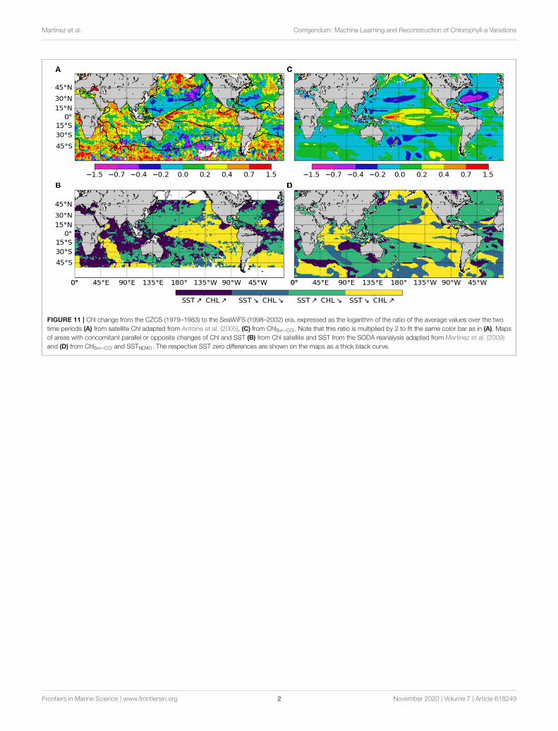
Martinez et al. Corrigendum: Machine Learning and Reconstruction of Chlorophyll-a Variations

FIGURE 11 | Chl change from the CZCS (1979–1983) to the SeaWiFS (1998–2002) era, expressed as the logarithm of the ratio of the average values over the two

time periods (A) from satellite Chl adapted from Antoine et al. (2005), (C) from ChlSvr−CCI. Note that this ratio is multiplied by 2 to fit the same color bar as in (A). Maps

of areas with concomitant parallel or opposite changes of Chl and SST (B) from Chl satellite and SST from the SODA reanalysis adapted from Martinez et al. (2009)

and (D) from ChlSvr−CCI and SSTNEMO. The respective SST zero differences are shown on the maps as a thick black curve.

Frontiers in Marine Science | www.frontiersin.org 2 November 2020 | Volume 7 | Article 618249