JOURNAL OF COMPUTATIONAL BIOLOGYVolume 13, Number 3, 2006© Mary Ann Liebert, Inc.Pp. 767–785

Reconstructing Ancestral Haplotypes with aDictionary Model

KRISTIN L. AYERS,1 CHIARA SABATTI,2,3 and KENNETH LANGE1,2,3

ABSTRACT

We propose a dictionary model for haplotypes. According to the model, a haplotype isconstructed by randomly concatenating haplotype segments from a given dictionary of seg-ments. A haplotype block is defined as a set of haplotype segments that begin and end withthe same pair of markers. In this framework, haplotype blocks can overlap, and the modelprovides a setting for testing the accuracy of simpler models invoking only nonoverlappingblocks. Each haplotype segment in a dictionary has an assigned probability and alternatespellings that account for genotyping errors and mutation. The model also allows for missingdata, unphased genotypes, and prior distribution of parameters. Likelihood evaluations relyon forward and backward recurrences similar to the ones encountered in hidden Markovmodels. Parameter estimation is carried out with an EM algorithm. The search for theoptimal dictionary is particularly difficult because of the variable dimension of the modelspace. We define a minimum description length criteria to evaluate each dictionary and usea combination of greedy search and careful initialization to select a best dictionary for agiven dataset. Application of the model to simulated data gives encouraging results. In areal dataset, we are able to reconstruct a parsimonious dictionary that captures patterns oflinkage disequilibrium well.

Key words: linkage disequilibrium, haplotype blocks, minimum description length, forward andbackwards algorithms, EM algorithm.

1. INTRODUCTION

Recent high-density genotyping of unrelated individuals has revealed limited haplotype di-versity and wide variation in linkage disequilibrium levels across the human genome (Patil et al.,

2001; Daly et al., 2001; Jeffreys et al., 2001; Reich et al., 2001; Gabriel et al., 2002). In many narrowgenome regions, a handful of conserved haplotypes account for almost all chromosomal variation. Haplo-types spanning several such adjacent regions often appear to be formed by concatenating short haplotypesegments drawn from nonoverlapping haplotype blocks. One can explain these observations by postu-lating that block boundaries coincide with recombination hot spots (Jeffreys et al., 2001; Cullen et al.,

1Department of Biomathematics, University of California, Los Angeles, CA 90095–1766.2Department of Human Genetics, University of California, Los Angeles, CA 90095–1766.3Department of Statistics, University of California, Los Angeles, CA 90095–1766.

767

768 AYERS ET AL.

2002; Gabriel et al., 2002; Kauppi et al., 2003) and that population bottlenecks and genetic drift act tolimit haplotype diversity (Wang et al., 2002). Although the evidence in favor of limited haplotype diversityis compelling, the hypothesis of universal block boundaries between conserved haplotype segments is, inour view, largely untested. The obvious danger is that the sharp boundaries currently seen are artifactsof the simple computational models used to analyze haplotype data. The goal of the present paper is toexplore a more complicated statistical model that captures limited haplotype diversity and varying patternsof linkage disequilibrium within the framework of overlapping block boundaries.A more sophisticated model has important implications for disease gene mapping. A better representation

of haplotype conservation will enable a more parsimonious selection of markers for genotyping. It will alsopromote greater statistical efficiency in association testing with cases and controls, if for no other reasonthan that it will lead to better haplotyping. The dictionary model we introduce is purely phenomenologicaland does not rely on detailed assumptions about the evolution of the underlying population. Buildinga model that incorporates evolutionary history is apt to be frustrated by great uncertainties and nearlyinsurmountable computational barriers. In contrast, our dictionary model permits fast, flexible parsing oflong haplotypes.

2. THE DICTIONARY MODEL

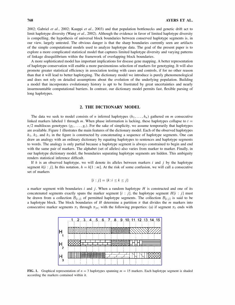
The data we seek to model consists of n inferred haplotypes (h1, . . . , hn) gathered on m consecutivelinked markers labeled 1 through m. When phase information is lacking, these haplotypes collapse to t =n/2 multilocus genotypes (g1, . . . , gt ). For the sake of simplicity, we assume temporarily that haplotypesare available. Figure 1 illustrates the main features of the dictionary model. Each of the observed haplotypesh1, h2, and h3 in the figure is constructed by concatenating a sequence of haplotype segments. One candraw an analogy with an ordinary dictionary by equating haplotypes to sentences and haplotype segmentsto words. The analogy is only partial because a haplotype segment is always constrained to begin and endwith the same pair of markers. The alphabet (set of alleles) also varies from marker to marker. Finally, inour haplotype dictionary model, the boundaries separating haplotype segments are hidden. This ambiguityrenders statistical inference difficult.If h is an observed haplotype, we will denote its alleles between markers i and j by the haplotype

segment h[i : j ]. In this notation, h = h[1 : m]. At the risk of some confusion, we will call a consecutiveset of markers

[i : j ] = {k : i ≤ k ≤ j}

a marker segment with boundaries i and j . When a random haplotype H is constructed and one of itsconcatenated segments exactly spans the marker segment [i : j ], the haplotype segment H [i : j ] mustbe drawn from a collection B[i:j ] of permitted haplotype segments. The collection B[i:j ] is said to bea haplotype block. The block boundaries of H determine a partition π that divides the m markers intoconsecutive marker segments π1 through π|π | with the following properties: (a) if segment π" ends with

FIG. 1. Graphical representation of n = 3 haplotypes spanning m = 15 markers. Each haplotype segment is shadedaccording the markers contained within it.

DICTIONARY MODEL FOR HAPLOTYPES 769

marker j , then segment π"+1 begins with marker j +1, (b) the first segment π1 begins with marker 1, and(c) the last segment π|π | ends with the last marker m. In most haplotype block models, only one partitionis feasible. With overlapping blocks, many different partitions are possible.As concrete examples of these conventions, haplotypes h1 and h2 in Fig. 1 share the marker segment

[8 : 10] and the particular haplotype segment h1[8 : 10] = h2[8 : 10] filling it. Haplotypes h2 and h3display different haplotype segments on marker segment [1 : 2], but these segments are drawn from thesame haplotype block B[1:2]. Finally, haplotype h2 has the marker segment [11 : 12] internal to the markersegment [11 : 13] of haplotype h3.Our dictionary model for haplotypes is inspired by an earlier dictionary model used to identify binding

sites of regulatory proteins along DNA sequences (Bussemaker et al., 2000; Sabatti and Lange, 2002). Tothe extent possible, we transfer the probability structure of these motif models to the haplotype model.Thus, in constructing a haplotype by concatenation from left to right, the added marker segments andhaplotype segments are independently chosen according to specific probabilities. To achieve maximummodel clarity, it is convenient to define marker segment probabilities, haplotype segment probabilities, andgenotyping error probabilities. Error probabilities cover not only genotyping error per se but also mutation.Because of errors, we must allow observed haplotypes to differ from theoretical haplotypes constructed byconcatenation.In constructing a random haplotype H , suppose that concatenation has brought us to the point where the

current marker segment ends with marker i −1. We then choose the next marker segment with conditionalprobability q[i:j ]. This mechanism forces the constraint

∑mj=i q[i:j ] = 1. Once we have chosen the next

marker segment [i : j ], we choose the next haplotype segment s from the haplotype block B[i:j ] withprobability rs . Again we have the constraint

∑s∈B[i:j ] rs = 1. A haplotype segment can be corrupted by

either genotyping error or mutation. The simplest error model postulates a product multinomial distributionand a uniform error rate εk across the ak alleles at marker k. If H is constructed using the segment s ∈ B[i:j ],then these assumptions yield the conditional probability

Pr(H [i : j ] = h[i : j ] | s) =j∏

k=i

Pr(H [k : k] = h[k : k] | s),

where

Pr(H [k : k] = h[k : k] | s) =

1 h[k : k] is missing1− εk h[k : k] = s[k : k]εk

ak − 1h[k : k] $= s[k : k] .

To express the probability Pr(H = h) succinctly, it is helpful to define

p(h[i : j ]) =∑

s∈B[i:j ]

rs Pr(H [i : j ] = h[i : j ] | s). (1)

The quantity p(h[i : j ]) is just the conditional probability of the observed haplotype segment h[i : j ]given H is constructed using marker segment [i : j ]. With this notation, the joint probability of a partitionπ and an observed haplotype h can be written as

Pr(H = h,π) =∏

[i:j ]∈πq[i:j ]p(h[i : j ]).

Because block boundaries are unobserved, the full probability of h is

Pr(H = h) =∑

π

∏

[i:j ]∈πq[i:j ]p(h[i : j ]), (2)

where the sum ranges over all possible partitions π .

770 AYERS ET AL.

The likelihood of a collection of independent haplotypes h1, . . . , hn factors into the likelihoods of theseparate haplotypes. If the data consists of independent multilocus genotypes, then the likelihood factorsover genotypes, but corresponding to each genotype there is an outer sum that increases the computationalcomplexity of likelihood evaluation. For a multilocus genotype g, let

Sg ={(h1, h2) : g = h1

h2

}

denote the set of maternal–paternal haplotype pairs compatible with g. If we assume that gametes combineat random, then the likelihood formula

Pr(G = g) =∑

(h1,h2)∈Sg

Pr(H1 = h1)Pr(H2 = h2) (3)

connects a random genotype G and its constituent haplotypes H1 and H2. With codominant markers andcomplete typing, consistent haplotype pairs differ only in phase. If parents are available, then most of thetime one can infer phase. Appendix I points out that the probability that a child’s phase is ambiguous ata codominant marker is at most 18 when both parents are typed and at most

14 when only one parent is

typed. If p heterozygous markers are unphased for the multilocus genotype g, then the sum (3) will rangeover 2p haplotype pairs.The likelihood expression (2) is computationally impractical as it stands. Generalizations of Baum’s

forward and backwards algorithms from the theory of hidden Markov chains offer a better avenue toevaluation. Let Ai be the event that some marker segment of the random haplotype H ends with marker i.In the forward algorithm, we calculate the joint probability

fi = Pr(H [1 : i] = h[1 : i], Ai)

of Ai and the event that H [1 : i] coincides with the partially observed haplotype h[1 : i]. The forwardalgorithm initializes f0 = 1 and computes the remaining fi from the recurrence

fi =min{d,i}∑

k=1fi−kq[i−k+1:i]p(h[i − k + 1 : i]) (4)

based on Equation (1) and an assumed maximum haplotype segment length d . The final probabilityfm is the likelihood of the haplotype H . The backwards algorithm computes the conditional probabilitybi = Pr(H [i : m] = h[i : m]|Ai−1) of the event H [i : m] = h[i : m] given the event Ai−1. We initializebm+1 = 1 and update the bi in the reverse order i = m, . . . , 1 via

bi =min{d,m−i+1}∑

k=1q[i:i+k−1]p(h[i : i + k − 1])bi+k. (5)

The final term b1 of the recurrence gives the likelihood of H .The conditional marker segment probabilities and haplotype segment probabilities do not fully convey

how often particular marker segments or haplotype segments are used in haplotype construction. However,the correct probabilities can be computed by a variation of the forward algorithm. As before, let Ai bethe event that a random haplotype has a marker segment ending with marker i. We can compute theprobabilities Pr(Ai) via the recurrence

Pr(Ai) =min{d,i}∑

k=1Pr(Ai−k)q[i−k+1:i] (6)

starting with the initial condition Pr(A0) = 1. This is just the forward algorithm with missing alleles at eachmarker. The probability that marker segment [i : j ] appears in a random haplotype is just Pr(Ai−1)q[i:j ].We will refer to this quantity as the marker segment probability. No backward probability is required

DICTIONARY MODEL FOR HAPLOTYPES 771

here because with probability 1 a partial haplotype ending at marker j is completed by concatenation.Similarly, the probability that a particular haplotype segment s in B[i:j ] appears in a random haplotype isPr(Ai−1)q[i:j ]rs . When we refer to the probability of s in the sequel, we will mean Pr(Ai−1)q[i:j ]rs ratherthan q[i:j ]rs .

3. DICTIONARY RECONSTRUCTION

The dictionary model presents two fundamental challenges: (a) estimation of the parameter vectors q, r ,and ε in a static dictionary with known haplotype segments; and (b) assembly of a dictionary of unknownhaplotype segments. We take up parameter estimation first.

3.1. Parameter estimationEvery observed haplotype h involves missing information represented by the partition π and the uncor-

rupted haplotype segments that fill the marker segments of π . With obvious missing information of thissort, the EM algorithm is the natural method of parameter estimation (Dempster et al., 1977). The completedata log likelihood required by the EM algorithm can be written in terms of the following quantities:

(a) Q[i:j ], the number of haplotypes using the marker segment [i : j ];(b) Rs , the number of haplotypes using the haplotype segment s;(c) Ti , the number of typing errors at marker i;(d) θ = (q, r, ε), the parameter vector.

Because each independent haplotype is constructed via a sequence of hidden multinomial trials, thecomplete data log likelihood reduces to

lnLcom(θ) =m∑

i=1

m∑

j=i

Q[i:j ] ln q[i:j ] +∑

s

Rs ln rs +m∑

i=1Ti ln εi

+m∑

i=1(T ∗

i − Ti) ln(1− εi )

up to an irrelevant constant, where T ∗i is the number of typing events at locus i. When there is no missing

data at marker i, clearly T ∗i = n. The E step of the EM algorithm calculates the conditional expectation

of lnLcom(θ) with respect to the observed data h = (h1, . . . , hn) and the current parameter vector θ". Forhidden multinomial trials, a simple counting argument correctly suggests that the M-step update for eachparameter can be expressed as a ratio of an expected number of successes to an expected number of trials,where all expectations are conditional on H = h and θ" (Lange, 2002). Hence, for s ∈ B[i:j ]

q"+1[i,j ] = E(Q[i:j ] | H = h, θ")m∑

k=i

E(Q[i:k] | H = h, θ")(7)

r"+1s = E(Rs | H = h, θ")E(Q[i:j ] | H = h, θ")

(8)

ε"+1i = E(Ti | H = h, θ")T ∗

i

. (9)

All of the conditional expectations appearing in these formulas are straightforward to calculate as explainedin Appendix II. Since expectations are additive, it clearly suffices to consider the case n = 1 of a single

772 AYERS ET AL.

haplotype. Using the results of the forward algorithm (4) and backward algorithm (5), we then have, forinstance,

E(Q[i:j ] | H = h, θ") = fi−1q[i:j ]p(h[i : j ])bj+1Pr(H = h)

. (10)

Similar expressions hold for the other conditional expectations figuring in the EM updates.In the presence of a multilocus genotype G, we have to amend these formulas slightly. If X is one of

the random variables featured in Equations (7) through (9), then we can always decompose X as the sumY1 + Y2, where Y1 is the contribution coming from the maternal haplotype H1 and Y2 is the contributioncoming from the paternal haplotype H2. The decomposition

E(X | G = g, θ") =∑

(h1,h2)∈Sg

Pr(H1 = h1 | θ")Pr(H2 = h2 | θ")Pr(G = g | θ")

×[E(Y1 | H1 = h1, θ

") + E(Y2 | H2 = h2, θ")

]

in conjunction with formulas such as (10) makes it possible to pass from haplotype data to multilocusgenotype data in forming EM updates.The EM algorithm also easily adapts to maximum a posteriori estimation. The simplest approach is to

introduce independent Dirichlet priors for each of the hidden multinomial distributions. These conjugatepriors add pseudo-counts to their corresponding multinomial categories (Lange, 2002). For instance, inestimating the error probability εi at marker i, we add the log beta prior

ln%(µi + νi ) − ln%(µi) − %(νi ) + (µi − 1) ln εi + (νi − 1) ln(1− εi )

to the log likelihood of the complete data. This sum survives intact through the E step of the EM algorithm.At the M step, it produces the revised update

ε"+1i = E(Ti | H = h, θ") + µi − 1n + µi + νi − 2

.

In other words, the counting interpretation of the EM prevails provided we add µi − 1 imaginary typingerrors and µi + νi − 2 imaginary trials to the hidden multinomial trials determining which allele is readat marker i. Similar considerations apply to maximum a posteriori estimation of the parameter vectors q

and r .

3.2. Dictionary selectionChoosing the number and kind of haplotype segments to include in a haplotype dictionary is a typical

model selection problem. Because fuller dictionaries always provide more flexible descriptions of dataand consequently higher likelihoods, one cannot rely simply on the comparison of models through theirmaximum likelihoods. Common sense suggests that statistical inference should be guided by considerationsof parsimony as well. Thus, it is customary to minimize an objective function that incorporates both amodel’s negative log likelihood and a penalty for model complexity. The two-stage version of the minimumdescription length (MDL) approach to inference provides a rationale for this procedure (Rissanen, 1978,1983; Hansen and Yu, 2001). In fact, MDL criteria have been previously suggested for the selectionof block boundaries in the analysis of haplotype data (Anderson and Novembre, 2003; Koivisto et al.,2003; Sheffi, 2004).In the MDL framework, one selects the probability model that requires the minimum number of bits

to describe (or transmit) both the model and the data. The number of bits necessary to transmit a modelreflects the complexity of the model. The number of bits necessary to transmit the data given a modeldepends on how well the model fits the data. Standard information theory arguments show that the shortestcode capable of transmitting a random message has length equal to the negative of the logarithm base 2

DICTIONARY MODEL FOR HAPLOTYPES 773

of the probability of the message. This means that we can measure the number of bits needed to transmitthe data given the model by the minimum of the negative log likelihood of the data. This yields the loglikelihood term in the MDL objective function.We must also evaluate the description length of the haplotype dictionary D behind the model. Each

haplotype block B[i:j ] of D involves |B[i:j ]|−1 independent parameters from the r vector and one parameterfrom the q vector. The q parameters involve m constraints, one for each marker. The loss of these m

parameters is compensated by the m error parameters. It follows that the number of independent parametersequals the size

|D| =m∑

i=1

m∑

j=i

|B[i:j ]|

of D. For n haplotypes, all of the parameters are real numbers measured with finite precision proportional to1/

√n, so at most 12 log2 n bits are required to encode each parameter. This takes care of the parameters. To

transmit a haplotype segment s, we must transmit the allele at each of its participating markers. Becausemarker k has ak alleles, it takes log2 ak bits to transmit one of its alleles. Although we also need totransmit the beginning and ending markers of each haplotype segment s, we will omit these relativelyminor contributions to model complexity. Summarizing both data and model contributions to the MDL,our objective function for comparing dictionaries is

Obj(D) = − 1ln 2

lnL(θ̂ | D) + 12|D| log2 n +

m∑

i=1

m∑

j=i

|B[i:j ]|j∑

k=i

log2 ak. (11)

Here the conversion factor 1/ ln 2 turns natural logarithms into logarithms base 2.With this objective function in hand, we still need a strategy for exploring model space. Our preferred

strategy combines heuristic construction of an initial dictionary with subsequent alternation of growing andpruning steps. For computational convenience, we retain all single-marker haplotype segments throughoutdictionary construction. At marker k, there are ak such trivial haplotype segments. This constraint ensuresthe compatibility of the dictionary with every conceivable haplotype even in the absence of genotypingerror.Because of the work involved in finding maximum likelihood estimates, it is unrealistic, on the one hand,

to start a search from an exhaustive dictionary containing all possible haplotype segments of length d orless. On the other hand, starting the search from the smallest dictionary with just the haplotype segmentsof length 1 tends to miss large conserved haplotype segments. It is better to make an educated guess of afairly large initial dictionary that is not heavily redundant. One way of assembling an initial dictionary isto choose two positive constants α and β and scan the data for common haplotype segments s (Patil et al.,2001; Johnson et al., 2001; Zhang et al., 2002b). When the empiric proportion of a segment s exceeds βand the empiric proportion of its associated haplotype block B[i:j ] exceeds α, s is included in the initialdictionary. If potential haplotype segments are visited in the order of their length and α and β are large,say .8 and .2, then this criterion tends to favor inclusion of just the short haplotype segments. On theother hand, taking α and β small, say .4 and .05, may produce a dictionary with tens of thousands ofentries. Such massive dictionaries contain almost every possible block and ensure that important haplotypesegments are not missed.It is useful to prune a massive initial dictionary first by heuristic methods that avoid likelihood evaluation.

Without committing ourselves to nonoverlapping blocks, we attempt to locate hard block boundaries intwo passes through the markers. The forward pass generates a subdictionary with nonoverlapping blocks;the reverse pass does likewise. However, taking the union of these two subdictionaries invariably yields apruned dictionary with overlapping blocks. The forward pass starts at marker 1 and progresses to marker m.Once we decide that a block ends with marker i − 1, we seek the marker segment [i : j ] defining thenext block. The decision to end the block with marker j depends on the number of haplotype segmentsnij in the dictionary that span the marker segment [i : j ]. At a true block boundary j , the differencedij = ni,j − ni,j+1 should be positive. If this condition holds and j > i + 2, then we declare j to bethe end of the current block. To discourage the creation of short blocks ending with j = i, i + 1, i + 2,and i + 3, we use the stronger stopping rule dij > 1. When we find the block boundary j , we drop all

774 AYERS ET AL.

haplotype segments that start at i and end before j , except, of course, the trivial ones. The reverse passoperates similarly but starts at marker m and progresses to marker 1.Once the initial dictionary is pruned by this heuristic method, we alternate more targeted growing and

pruning steps until the current dictionary stabilizes. Growing may well restore some of the haplotypesegments deleted in the initial pruning. To grow the dictionary, we must identify candidate haplotypesegments to add. The most fruitful approach is to concatenate two adjacent haplotype segments, s and t ,already in the dictionary. Because trivial haplotype segments are always retained, it is possible to growhaplotype segments laboriously one marker at a time. To decide whether to add the concatenated haplotypesegment st to the current dictionary, we use the expected number E(Rst | H = h, θ̂) of times st appearsin the haplotype data h. This criterion is given by

E(Rst | H = h, θ̂) =hn∑

h=h1

fi−1q[i:k]p(h[i:k])q[k+1:j ]p(h[k+1:j ])bj+1Pr(H = h)

,

where s spans the marker segment [i : k] and t spans the marker segment [k + 1 : j ]. It is instructive tocompare this conditional expectation to the theoretical probability

cst = Pr(Ai−1)q[i:k]rsq[k+1:j ]rt

that the two haplotype segments s and t co-occur in a random haplotype. Since the actual number of timesthe segment st appears follows a binomial distribution, we define the score

τst = E(Rst | H = h, θ̂) − ncst√ncst (1− cst )

and add the segment st to the dictionary whenever τst falls above a user designated cutoff.To prune the dictionary, we use a combination of global and local tactics. After each round of growing,

we first attempt to prune haplotype segments en masse by pruning blocks. The current blocks are orderedby their corresponding conditional expectations E(Q[i:j ] | H = h, θ) evaluated at the maximum likelihoodestimate θ = θ̂ . An exception is made for the trivial blocks, which are forced to come first. The resultingorder defines a sequence of nested subdictionaries, and bisection is applied to find the subdictionary withthe lowest value of the objective function (11). Assuming that the objective function first declines and thenrises as we progress from the smallest to the largest subdictionary, bisection makes it possible to pruneseveral haplotype blocks simultaneously. We also apply bisection to drop haplotype segments in chunksrather than haplotype blocks in chunks. The nontrivial haplotype segments s are first ordered by theirconditional expectations E(Rs | H = h, θ̂).Local pruning is achieved by dropping individual haplotype segments rather than entire haplotype blocks.

We first prune all haplotype segments s with low conditional probabilities rs , say, less than 10−3. We thenconsider haplotype segments u nested within larger segments v. For example, if the concatenated segmentst is added during the previous round of growing, then s and t will be nested within st unless they havealready been pruned. Let Cu denote the collection of segments v strictly containing u. If nu counts thenumber of observed haplotypes that agree with u on the marker segment defining u and mu counts thenumber of observed haplotypes that agree with some v in Cu on the marker segment defining v, thencomparison of nu and mu conveys how redundant u is. Hence, we drop u from the current dictionary ifthe ratio nu/mu falls below a user defined cutoff γ . For nested pairs u ⊂ v of comparable length, it maybe better to drop v rather than u. In such cases, we use the values Obj(D ∪ {u} ∪ {v}), Obj(D ∪ {u}),and Obj(D ∪ {v}) of the objective function to reach a decision, where D is the current dictionary omittingu and v. Alternation of growing and pruning steps stops when there are no further promising haplotypesegments to add.The search strategy just described is clearly heuristic. It is based on experience and tinkering, and by no

means is it guaranteed to converge to the optimal dictionary. However, in practice, it successfully identifiesparsimonious dictionaries that offer accurate descriptions of the data.

DICTIONARY MODEL FOR HAPLOTYPES 775

3.3. Software implementationOur computer program HAPPER implements the EM algorithm and the dictionary selection procedure.

The user designates values for the parameters α, β, the threshold τ for adding haplotype segments, andthe threshold γ for dropping nested haplotype segments. One may construct a better dictionary by playingwith these parameters. HAPPER outputs the final marker segments [i : j ], their probabilities Pr(Ai)q[i:j ],the alleles of each haplotype segment s in the corresponding block B[i:j ], and the conditional probabilityrs of s given the block B[i:j ]. To provide a snapshot of the linkage disequilibrium patterns in the data asexplained by the model, HAPPER computes the co-occurrence probability mij that markers i and j arefound on the same haplotype segment. These probabilities are output as a matrix M = (mij ) ready fortwo-dimensional display. Last of all, when the data consists of multilocus genotypes, HAPPER provides foreach observed genotype the most likely pair of haplotypes and its probability. The program runs fairly faston phased data, constructing a dictionary in approximately 5 minutes for 20 markers and 200 genotypesand in 1 hour for 100 markers and 100 genotypes. For fully unphased data, the program has to sum overevery possible phase in likelihood evaluation. A dataset of 100 genotypes and 20 markers accordinglytakes several days to construct a dictionary.

4. RESULTS

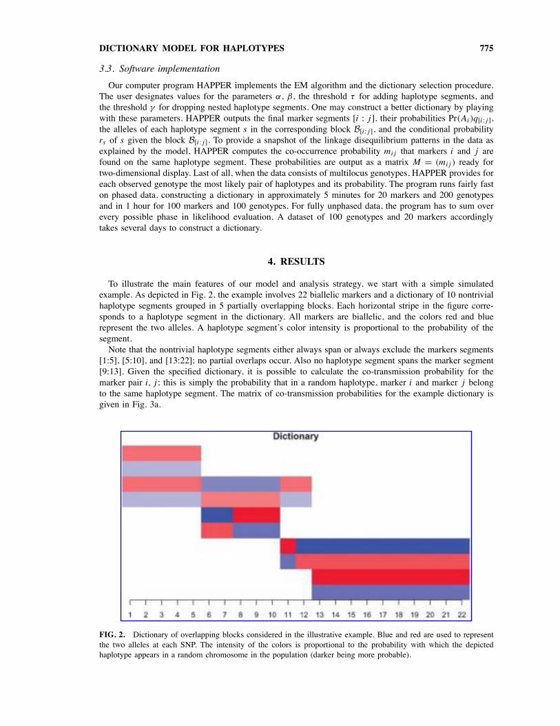
To illustrate the main features of our model and analysis strategy, we start with a simple simulatedexample. As depicted in Fig. 2, the example involves 22 biallelic markers and a dictionary of 10 nontrivialhaplotype segments grouped in 5 partially overlapping blocks. Each horizontal stripe in the figure corre-sponds to a haplotype segment in the dictionary. All markers are biallelic, and the colors red and bluerepresent the two alleles. A haplotype segment’s color intensity is proportional to the probability of thesegment.Note that the nontrivial haplotype segments either always span or always exclude the markers segments

[1:5], [5:10], and [13:22]; no partial overlaps occur. Also no haplotype segment spans the marker segment[9:13]. Given the specified dictionary, it is possible to calculate the co-transmission probability for themarker pair i, j ; this is simply the probability that in a random haplotype, marker i and marker j belongto the same haplotype segment. The matrix of co-transmission probabilities for the example dictionary isgiven in Fig. 3a.

FIG. 2. Dictionary of overlapping blocks considered in the illustrative example. Blue and red are used to representthe two alleles at each SNP. The intensity of the colors is proportional to the probability with which the depictedhaplotype appears in a random chromosome in the population (darker being more probable).

776 AYERS ET AL.

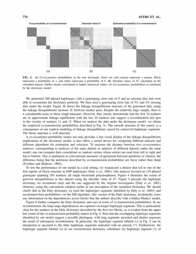
FIG. 3. (a) Co-occurrence probabilities in the true dictionary. Each row and column represent a marker. Blackrepresents a probability of 1, and white represents a probability of 0. (b) Absolute values of D′ calculated on thesimulated dataset. Darker shades correspond to higher numerical values. (c) Co-occurrence probabilities as estimatedby the dictionary model.

We generated 200 phased haplotypes with a genotyping error rate of 0 and no missing data and wereable to reconstruct the dictionary perfectly. We then used a genotyping error rate of 5% and 5% missingdata under the model. Figure 3b shows the linkage disequilibrium structure of the generated data, usingthe linkage disequilibrium measure D′ between marker pairs. Despite the relatively large sample, there isa considerable noise in these rough measures. However, they clearly demonstrate that the first 10 markersare in approximate linkage equilibrium with the last 10 markers and suggest a recombination hot spotin the vicinity of markers 11 and 12. When we analyze the data under the dictionary model, we obtainthe empirical co-transmission probabilities described in Fig. 3c. The smooth structure of this matrix is aconsequence of our explicit modeling of linkage disequilibrium caused by conserved haplotype segments.The block structure is well detected.A co-occurrence probability matrix not only provides a fast visual display of the linkage disequilibrium

implications of the dictionary model, it also offers a useful device for comparing different datasets anddifferent algorithms for estimation and selection. To measure the distance between two co-occurrencematrices, corresponding to analyses of the same dataset or analyses of different datasets under the samemodel, one can compute their correlations as random vectors whose entries are read from left to right andtop to bottom. This is analogous to conventional measures of agreement between partitions or clusters, thedifference being that the partitions described by co-transmission probabilities are fuzzy rather than sharp(Fowlkes and Mallows, 1983).To test the performance of our model in a real setting, we reanalyzed a dataset that led to one of the

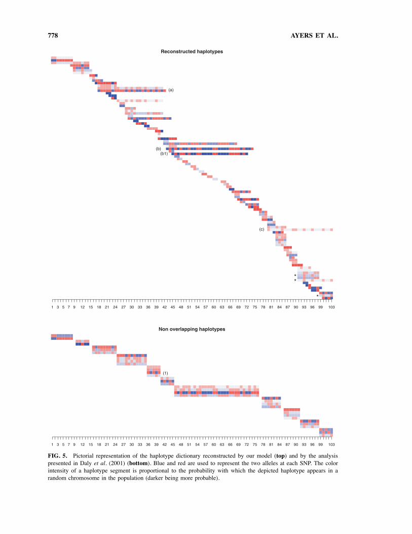
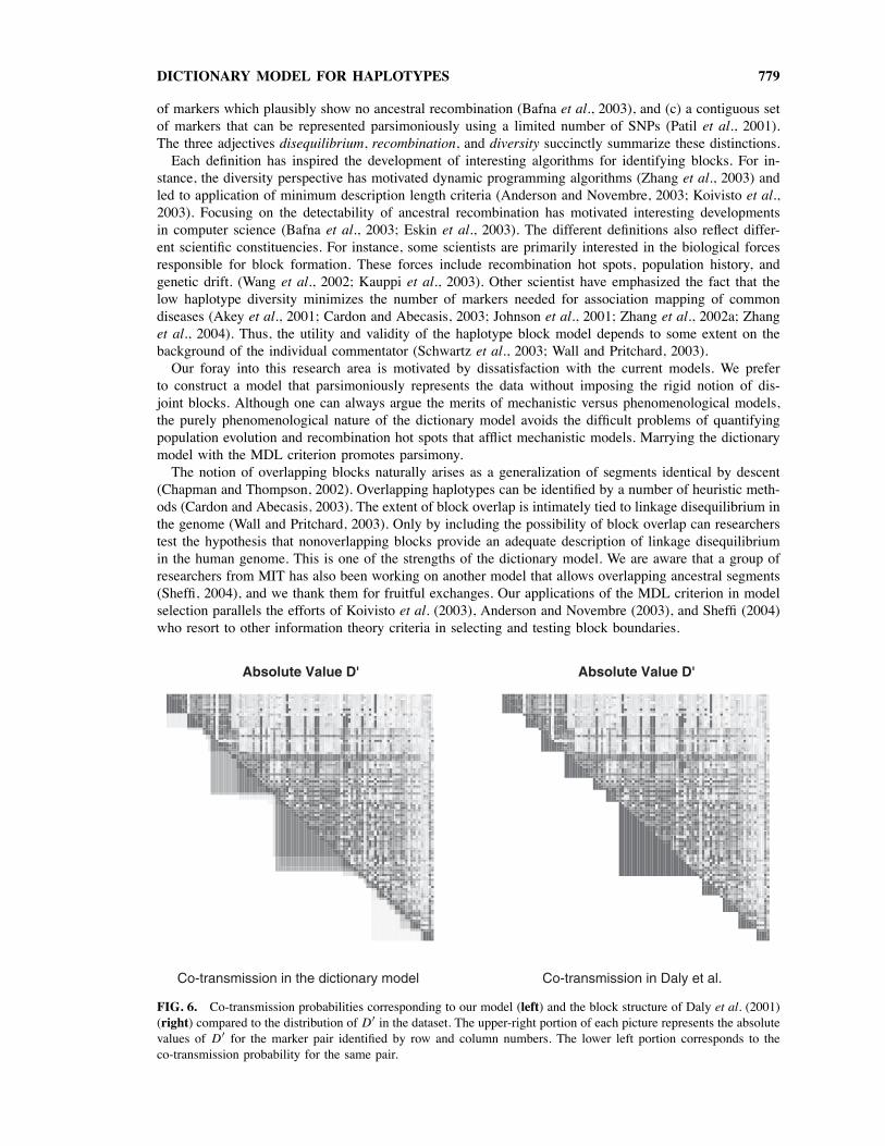
first reports of block structure in SNP haplotypes (Daly et al., 2001). Our analysis focused on 129 phasedgenotypes spanning 103 markers, all single nucleotide polymorphisms. Figure 4 illustrates the extent ofpairwise disequilibrium in this dataset using the absolute value of D′. Figure 5 presents the haplotypedictionary we reconstruct (top) and the one suggested by the original investigators (Daly et al., 2001)(bottom), using the conventions adopted earlier in our description of the simulated dictionary. We shouldclarify that in the Daly dictionary we used the haplotypes segments identified by Daly et al. (2001) andreestimated their probabilities via the EM algorithm. Our version of the Daly dictionary, incidentally, losesany information on the dependencies across blocks that the authors describe with a hidden Markov model.Figure 6 further compares the Daly dictionary and ours in terms of co-transmission probabilities. In our

reconstruction, the long range dependencies are captured via longer haplotype segments. This is particularlyclear for the markers in the Daly dictionary described by the first two blocks, as is evident from the upperleft corner of the co-transmission probability matrix in Fig. 6. Note that the overlapping haplotype segmentsidentified by our model suggest a possible phylogeny, with long segments ancestral and shorter segmentsthe result of subsequent recombination. In particular, the haplotype segment labeled (c) in Fig. 5 can beinterpreted as ancestral to the other haplotype segments indicated with an asterisk (*). Furthermore, thehaplotype segment labeled (a) in our reconstructed dictionary substitutes for haplotype segment (1) of

DICTIONARY MODEL FOR HAPLOTYPES 777

FIG. 4. Absolute values of the D′ measure on the dataset obtained from Daly et al. (2001).

the Daly dictionary. Haplotype segments (b) and (b1) in our reconstructed dictionary are quite similar,differing only by a probable mutation at position 49. The MDL criterion strongly favors our dictionarywith overlapping haplotypes to the Daly dictionary, the difference in the objective function (11) being1,642. Thus, a dictionary with overlapping blocks appears to offer a substantially better description of thedata than one with nonoverlapping blocks.

5. DISCUSSION

A few years ago, geneticists noticed blocklike patterns of linkage disequilibrium in several sequencesof closely spaced SNPs (Daly et al., 2001; Patil et al., 2001; Reich et al., 2001; Gabriel et al., 2002).This observation spurred development of novel statistical methods and massive data gathering, eventuallyprompting founding of The International Hapmap Consortium (2003). The extensive literature on haplotypeblocks defies brief summary. Scientists have approached the subject of haplotype geography with differentscientific objectives, leading to varied definition of blocks, contrasting interpretations of their nature, anddifferent strategies to identify them (Schwartz et al., 2003). The definitions of a block include (a) acontiguous set of markers for which the average value of the disequilibrium index D′ exceeds somepredetermined threshold (Daly et al., 2001; Reich et al., 2001; Gabriel et al., 2002), (b) a contiguous set

778 AYERS ET AL.

FIG. 5. Pictorial representation of the haplotype dictionary reconstructed by our model (top) and by the analysispresented in Daly et al. (2001) (bottom). Blue and red are used to represent the two alleles at each SNP. The colorintensity of a haplotype segment is proportional to the probability with which the depicted haplotype appears in arandom chromosome in the population (darker being more probable).

DICTIONARY MODEL FOR HAPLOTYPES 779

of markers which plausibly show no ancestral recombination (Bafna et al., 2003), and (c) a contiguous setof markers that can be represented parsimoniously using a limited number of SNPs (Patil et al., 2001).The three adjectives disequilibrium, recombination, and diversity succinctly summarize these distinctions.Each definition has inspired the development of interesting algorithms for identifying blocks. For in-

stance, the diversity perspective has motivated dynamic programming algorithms (Zhang et al., 2003) andled to application of minimum description length criteria (Anderson and Novembre, 2003; Koivisto et al.,2003). Focusing on the detectability of ancestral recombination has motivated interesting developmentsin computer science (Bafna et al., 2003; Eskin et al., 2003). The different definitions also reflect differ-ent scientific constituencies. For instance, some scientists are primarily interested in the biological forcesresponsible for block formation. These forces include recombination hot spots, population history, andgenetic drift. (Wang et al., 2002; Kauppi et al., 2003). Other scientist have emphasized the fact that thelow haplotype diversity minimizes the number of markers needed for association mapping of commondiseases (Akey et al., 2001; Cardon and Abecasis, 2003; Johnson et al., 2001; Zhang et al., 2002a; Zhanget al., 2004). Thus, the utility and validity of the haplotype block model depends to some extent on thebackground of the individual commentator (Schwartz et al., 2003; Wall and Pritchard, 2003).Our foray into this research area is motivated by dissatisfaction with the current models. We prefer

to construct a model that parsimoniously represents the data without imposing the rigid notion of dis-joint blocks. Although one can always argue the merits of mechanistic versus phenomenological models,the purely phenomenological nature of the dictionary model avoids the difficult problems of quantifyingpopulation evolution and recombination hot spots that afflict mechanistic models. Marrying the dictionarymodel with the MDL criterion promotes parsimony.The notion of overlapping blocks naturally arises as a generalization of segments identical by descent

(Chapman and Thompson, 2002). Overlapping haplotypes can be identified by a number of heuristic meth-ods (Cardon and Abecasis, 2003). The extent of block overlap is intimately tied to linkage disequilibrium inthe genome (Wall and Pritchard, 2003). Only by including the possibility of block overlap can researcherstest the hypothesis that nonoverlapping blocks provide an adequate description of linkage disequilibriumin the human genome. This is one of the strengths of the dictionary model. We are aware that a group ofresearchers from MIT has also been working on another model that allows overlapping ancestral segments(Sheffi, 2004), and we thank them for fruitful exchanges. Our applications of the MDL criterion in modelselection parallels the efforts of Koivisto et al. (2003), Anderson and Novembre (2003), and Sheffi (2004)who resort to other information theory criteria in selecting and testing block boundaries.

FIG. 6. Co-transmission probabilities corresponding to our model (left) and the block structure of Daly et al. (2001)(right) compared to the distribution of D′ in the dataset. The upper-right portion of each picture represents the absolutevalues of D′ for the marker pair identified by row and column numbers. The lower left portion corresponds to theco-transmission probability for the same pair.

780 AYERS ET AL.

One of the attractive features of the dictionary model is that it handles unphased data. A few other recentpapers also discuss the reconstruction of haplotype blocks from genotypes (Schwartz et al., 2002; Zhanget al., 2004; Halperin and Eskin, 2004; Greenspan and Geiger, 2004). Our implementation of the dictionarymodel is limited to about 16 markers on completely unphased data. In the absence of phase information,likelihood evaluation is hindered by the need to sum over all possible phases. Fortunately, the EM algorithmscales no worst than likelihood evaluation. Excoffier and Slatkin (1995) have noted similar computationalbarriers. The phase problem and the presence of overlapping blocks make exploration of dictionary spacecomputationally intensive despite the remarkable efficiency of likelihood evaluation via the forward andbackward algorithms and search via the EM algorithm. As a consequence, the dictionary model is bestsuited for analyzing in detail a specific chromosome region rather than tiling an entire genome. Thisshould not be a serious limitation because most geneticists are in interested in narrow regions of linkagedisequilibrium.

APPENDIX I: MULTILOCUS GENOTYPES

Consider a marker locus with n codominant alleles labeled 1, . . . , n. Most genotypic combinations of amother–father–child trio make it possible to infer which allele the mother contributes to the child and whichallele the father contributes to the child. It turns out that the only ambiguous case occurs when all threemembers of the trio share the same heterozygous genotype i/j . The probability of such a configuration is(2pipj )

2 12 , where pi and pj are the population frequencies (proportions) of alleles i and j . This formula

follows from (a) the independence of the parents’ genotypes, (b) Hardy–Weinberg equilibrium, and (c) aprobability of 1

2 that one of them transmits to the child an i allele and the other transmits a j allele.Using these configuration formulas, we can express the probability that the trio’s genotypes do not permitinference of the origin of both of the child’s alleles as the sum

f (p) =∑

i<j

(2pipj )2 12.

Lange (2004)) shows that f (p) attains it maximum of 18 when two of the frequencies pi equal 12 and theremaining frequencies equal 0.Rather than repeat that proof here, we would like to consider the slightly different situation where the

genotype of one of the parents, say the father, is unknown. What is the probability that we cannot determinethe parental contributions to the child given only the mother’s genotype and the child’s genotype? Againthe only ambiguous case occurs when the mother and the child have the same heterozygous genotypes i/j .It is clear that a mother with heterozygous genotype i/j is equally likely to pass either allele i or allele j .If she passes allele i, then the father must pass allele j . Under the random union of gametes model thatwe have implicitly adopted, the father passes allele j with probability pj . Hence,

Pr(child is i/j |mother is i/j) = 12pi + 1

2pj ,

and the probability that the mother and child have the same heterozygous genotype reduces to the sum

g(p) =∑

i<j

2pipj

(12pi + 1

2pj

)

=∑

i<j

[p2i pj + pip2j ]

=∑

i

∑

j $=i

p2i pj

=∑

i

p2i (1− pi).

DICTIONARY MODEL FOR HAPLOTYPES 781

For n = 2, the function g(p) = p21(1 − p1) + (1 − p1)2p1 = p1(1 − p1) attains its maximum of 14

when p1 = p2 = 12 . For general n, this suggests that the maximum occurs when all pi = 1

n . However, atthis point, g(p) equals n−1

n2, which is strictly less than 1

4 for n ≥ 3. This failure leads us to guess that themaximum of 14 occurs on a boundary where all but two of the pi = 0. By symmetry, we can assume thatthe sequence pi is increasing in i. Under this assumption, we now demonstrate that we can increase g(p)

by incrementing p2 by q ∈ [0, p1] at the expense of decrementing p1 by q. If we define the perturbedvalue of g(p) by

h(q) = (p1 − q)2(1− p1 + q) + (p2 + q)2(1− p2 − q) +n∑

j=3p2j (1− pj ),

then it is evident that its derivative

h′(q) = (p1 − q)2 − 2(p1 − q)(1− p1 + q) − (p2 + q)2 + 2(p2 + q)(1− p2 − q)

= (p2 − p1 + 2q)[2− 3(p1 + p2)].

For n ≥ 3, our order assumption 0 < q ≤ p1 . . . ≤ pn implies that p1 + p2 ≤ 23 , so both of the factors

defining h′(q) are nonnegative. It follows that we can reduce p1 to 0 and increase p2 to p1 + p2 withoutdecreasing g(p). In general, we should keep discarding the lowest positive pj until only pn−1 and pn

survive. At this juncture, we maximize g(p) by taking pn−1 = pn = 12 .

The computational complexity of likelihood evaluation under the dictionary model is dominated by themultilocus genotype with the maximum number of possible phases. Hence, it is instructive to examinethe worst case of m SNPs, each with two equally frequent alleles. Given fully typed parents, the num-ber of phase ambiguities Xi for the ith multilocus genotype is binomially distributed with m trials andsuccess probability 1

8 . Assuming that t independent multilocus genotypes are observed, the maximumZ = max{X1, . . . , Xt } has distribution function

Pr(Z ≤ z) = Pr(X1 ≤ z)t .

If m is reasonable large, then X1 is approximately normal with mean m8 and variance

7m64 and

Pr(X1 ≤ z) ≈ +(

z − m/8√7m/64

),

where +(z) is the standard normal distribution function. The median value of Z, therefore, approximatelysatisfies the identity

12

= +(

zmedian − m/8√7m/64

)t

,

whose solution is

zmedian = m

8+

√7m64+[−1]

(2−1/t

),

where +[−1](z) is the functional inverse of +(z). Figure 7 depicts the level curves of zmedian as a functionof m and t . Computation tends to bog down when the maximum number of phase uncertainties exceeds12. This optimistic conclusion must be tempered by the fact that most datasets contain a high percentageof partially typed markers.

782 AYERS ET AL.

FIG. 7. Level curves of zmedian for m markers and t multilocus genotypes.

APPENDIX II: DERIVATION OF EM UPDATES

Because the complete data likelihood Lcom(θ) is a product over the observations, we examine thelikelihood of a single observed genotype g. The complete data reveal the haplotype pair (h1, h2) underlyingg and the partitions π1 and π2 segmenting h1 and h2. The complete data likelihood can be written interms of the following indicator random variables:

W(h1,h2) ={1 if observation g has phased genotype (h1, h2)0 otherwise,

V c[i:j ] =

{1 if marker segment [i : j ] occurs in haplotype hc

0 otherwise,

Fcs =

{1 if haplotype segment s occurs in haplotype hc

0 otherwise,

Ucs,k =

{1 if hc[k : k] = s[k : k]0 otherwise,

Zcs,k =

{1 if hc[k : k] $= s[k : k],0 otherwise.

If locus k is untyped, then we put Ucs,k = Zc

s,k = 0. For a particular observation g, we can write thecomplete data likelihood as

Lg(θ) =∏

(h1,h2)

2∏

c=1

∏

πc

∏

[i:j ]∈πc

q[i:j ]

∏

s∈B[i:j ]

rs

j∏

k=i

(1− εk)Ucs,k

(εk

ak − 1

)Zcs,k

Fc

s

V c[i:j ]

W(h1,h2)

.

DICTIONARY MODEL FOR HAPLOTYPES 783

Taking logarithms yields the complete data log likelihood

Lg(θ) =∑

(h1,h2)

W(h1,h2)

2∑

c=1

∑

πc

∑

[i:j ]∈πc

× V c[i:j ]

ln q[i:j ] +∑

s∈B[i:j ]

Fcs

ln rs +j∑

k=i

Ucs,k ln(1− εk) + Zc

s,k

(εk

ak − 1

)

.

The E step of the EM algorithm is carried to completion by noting that the product of two indicators isan indicator and the conditional expectation of an indicator is a conditional probability.The surrogate function produced by the E step separates the parameters and allows us to deal with them

in batches. Each batch gives rise to a multinomial or binomial log likelihood of the form∑

i ui ln bi , whereui and bi are the fractional count and probability assigned to category i. It is well known that such a sumis maximized subject to bi ≥ 0 and

∑i bi = 1 by taking

b̂i = ui∑

j

uj

.

This specifies the M step of the EM algorithm in broad outline. In the specific cases of the updates (7),(8), and (9), the reader can check the identities

E(Q[i:j ] | G = g, θ") =∑

(h1,h2)

2∑

c=1

∑

πc

E(W(h1,h2)Vc[i:j ] | G = g, θ") (12)

E(Rs | G = g, θ") =∑

(h1,h2)

2∑

c=1

∑

πc

E(W(h1,h2)Vc[i:j ]F

cs | G = g, θ") (13)

E(Tk | G = g, θ") =∑

(h1,h2)

2∑

c=1

∑

πc

∑

[i:j ]∈πc

∑

s∈B[i:j ]

(14)

E(W(h1,h2)Vc[i:j ]F

cs Zc

s,k | G = g, θ")

connecting the conditional expected counts to the conditional probabilities for a single genotype g. It isworth stressing that the conditional probabilities shown above are efficiently computed by the forward–backward sandwich equations featured in the text. All three formulas (12), (13), and (14) must be summedover the t possible genotypes.

ACKNOWLEDGMENTS

This research supported in part by NIH training grant HG02536(KLA), NSF grant DMS0239427(CS),and USPHS grants GM53275(CS,KL) and MH59490(KL).

REFERENCES

Akey, J., Jin, L., and Xiong, M. 2001. Haplotypes vs. single marker linkage disequilibrium tests: What do we gain?Eur. J. Human Genet. 9, 291–300.

Anderson, E.C., and Novembre, J. 2003. Finding haplotype block boundaries by using the minimum-description-lengthprinciple. Am. J. Human Genet. 73, 336–354.

784 AYERS ET AL.

Bafna, V., Gusfield, D., Lancia, G., and Yooseph, S. 2003. Haplotyping as perfect phylogeny: A direct approach.J. Comp. Biol. 10, 323–340.

Bussemaker, H.J., Li, H., and Siggia, E.D. 2000. Building a dictionary for genomes: Identification of presumptiveregulatory sites by statistical analysis. Proc. Natl. Acad. Sci. USA 97, 10096–10100.

Cardon, L., and Abecasis, G. 2003. Using haplotype blocks to map human complex trait loci. Trends Genet. 19,135–140.

Chapman, N.H., and Thompson, E.A. 2002. The effect of population history on the lengths of ancestral chromosomesegments. Genetics 162, 449–458.

Cullen, M., Perfetto, S.P., Klitz, W., Nelson, G., and Carrington, M. 2002. High-resolution patterns of meiotic recom-bination across the human major histocompatibility complex. Am. J. Human Genet. 71, 759–776.

Daly, M.J., Rioux, J.D., Schaffner, S.F., Hudson, T.J., and Lander, E.S. 2001. High-resolution haplotype structure inthe human genome. Nature Genet. 29, 229–232.

Dempster, A.P., Laird, N.M., and Rubin, D.B. 1977. Maximum likelihood from incomplete data via the EM algorithm.J. Roy. Statist. Soc. 39, 1–38.

Eskin, E., Halperin, E., and Karp, R. 2003. Efficient reconstruction of haplotype structure via perfect phylogeny.J. Bioinformatics Comp. Biol. 1, 1–20.

Excoffier, L., and Slatkin, M. 1995. Maximum likelihood estimation of molecular haplotype frequencies in a diploidpopulation. Mol. Biol. Evol. 12(5), 921–927.

Fowlkes, E., and Mallows, C. 1983. A method for comparing two hierarchical clusterings. J. Am. Stat. Assoc. 78,553–569.

Gabriel, S.B., Schaffner, S.F., Nguyen, H., Moore, J.M., Roy, J., Blumenstiel, B., Higgins, J., DeFelice, M., Lochner,A., Faggart, M., Liu-Cordero, S.N., Rotimi, C., Adeyemo, A., Cooper, R., Ward, R., Lander, E.S., Daly, M.J., andAltshuler, D. 2002. The structure of haplotype blocks in the human genome. Science 296, 2225–2229.

Greenspan, G., and Geiger, D. 2004. Model-based inference of haplotype block variation. J. Comp. Biol. 11, 495–506.Halperin, E., and Eskin, E. 2004. Haplotype reconstruction from genotype data using imperfect phylogeny. Bioinfor-matics 20, 1842–1849.

Hansen, M., and Yu, B. 2001. Model selection and the principle of minimum description length. J. Am. Stat. Assoc.96, 746–774.

The International Hapmap Consortium. 2003. The International HapMap Project. Nature 426, 789–796.Jeffreys, A.J., Kauppi, L., and Neumann, R. 2001. Intensely punctate meiotic recombination in the class II region ofthe major histocompatibility complex. Nature Genet. 29, 217–221.

Johnson, G.C., Esposito, L., Barratt, B.J., Smith, A.N., Heward, J., Genova, G.D., Ueda, H., Cordell, H.J., Eaves, I.A.,Dudbridge, F., Twells, R.C., Payne, F., Hughs, W., Nutland, S., Stevens, H., Carr, P., Tuomilehto-Wolf, E., Tuomilehto,J., Gough, S.C., Clayton, D.G., and Todd, J.A. 2001. Haplotype tagging for the identification of common diseasegenes. Nature Genet. 29, 233–237.

Kauppi, L., Sajantila, A., and Jeffreys, A.J. 2003. Recombination hotspots rather than population history dominatelinkage disequilibrium in the MHC class II region. Human Mol. Genet. 12, 33–40.

Koivisto, M., Perola, M., Varilo, T., Hennah, W., Ekelund, J., Lukk, M., Peltonen, L., Ukkonen, E., and Mannila, H.2003. An MDL method for finding haplotype blocks and for estimating the strength of haplotype block boundaries.Proc. 8th Pac. Symp. Biocomputing (PSB ’03) 12, 502–513.

Lange, K. 2002. Mathematical and Statistical Methods For Genetic Analysis, Springer-Verlag, New York.Lange, K. 2004. Optimization, Springer-Verlag, New York.Patil, N., Berno, A.J., Hinds, D.A., Barrett, W.A., Doshi, J.M., Hacker, C.R., Kautzer, C.R., Lee, D.H., Marjoribanks,C., McDonough, D.P., Nguyen, B.T., Norris, M.C., Sheehan, J.B., Shen, N., Stern, D., Stokowski, R.P., Thomas, D.J.,Trulson, M.O., Vyas, K.R., Frazer, K.A., Fodor, S.P.A., and Cox, D.R. 2001. Blocks of limited haplotype diversityrevealed by high-resolution scanning of human chromosome 21. Science 294, 1719–1724.

Reich, D.E., Cargill, M., Bolk, S., Ireland, J., Sabeti, P.C., Richter, D.J., Lavery, T., Kouyoumjian, R., Farhadian, S.F.,Ward, R., and Lander, E.S. 2001. Linkage disequilibrium in the human genome. Nature 411, 199–204.

Rissanen, J. 1978. Modeling by shortest data description. Automatica 14, 465–471.Rissanen, J. 1983. A universal prior for integers and estimation by minimum description length. Ann. Statist. 11,416–431.

Sabatti, C., and Lange, K. 2002. Genomewise motif identification using a dictionary model. IEEE Proc. 90, 1803–1810.

Schwartz, R., Clark, A.G., and Istrail, S. 2002. Methods for inferring block-wise ancestral history from haploidsequences. Algorithms in Bioinformatics, Lecture Notes in Computer Science 2452, 44–59, Springer-Verlag, Berlin.

Schwartz, R., Halldorsson, B., Bafna, V., Clark, A., and Istrail, S. 2003. Robustness of inference of haplotype blockstructure. J. Comp. Biol. 10, 13–19.

Sheffi, J. 2004. An HMM-based boundary-flexible model of human haplotype variation. Master’s thesis, MIT, Depart-ments of Electrical Engineering and Computer Science.

DICTIONARY MODEL FOR HAPLOTYPES 785

Wall, J.D., and Pritchard, J. 2003. Assessing the performance of the haplotype block model of linkage disequilibrium.Am. J. Human Genet. 73, 502–515.

Wang, N., Akey, J.M., Zhang, K., Chakraborty, R., and Jin, L. 2002. Distrubution of recombination crossovers and theorigin of haplotype blocks: The interplay of population history, recombination, and mutation. Am. J. Human Genet.71, 1227–1234.

Zhang, K., Calabreses, P., Nordborg, M., and Sun, F. 2002a. Haplotype block structure and its applications to associationstudies: Power and study designs. Am. J. Human Genet. 71, 1386–1394.

Zhang, K., Deng, M., Chen, T., Waterman, M.S., and Sun, F. 2002b. A dynamic programming algorithm for haplotypeblock partitioning. Proc. Natl. Acad. Sci. USA 99, 7335–7339.

Zhang, K., Qin, Z.S., Liu, J.S., Chen, T., Waterman, M.S., and Sun, F. 2004. Haplotype block partitioning and tagSNP selection using genotype data and their applications to association studies. Genome Res. 14, 908–916.

Zhang, K., Sun, F., Waterman, M.S., and Chen, T. 2003. Haplotype block partition with limited resources and appli-cations to human chromosome 21 haplotype data. Am. J. Human Genet. 73, 63–73.

Address correspondence to:Kenneth Lange

Department of Human GeneticsUCLA School of Medicine

695 Charles E. Young Drive SouthLos Angeles, California 90095-7088

E-mail: klange@ucla.edu