recompression of hadamard products of tensors ... - sma...
TRANSCRIPT

Recompression of Hadamard Products
of Tensors in Tucker Format
Daniel Kressner* Lana Perisa
June 20, 2017
Abstract
The Hadamard product features prominently in tensor-based algorithms in sci-entific computing and data analysis. Due to its tendency to significantly increaseranks, the Hadamard product can represent a major computational obstacle in algo-rithms based on low-rank tensor representations. It is therefore of interest to developrecompression techniques that mitigate the effects of this rank increase. In this work,we investigate such techniques for the case of the Tucker format, which is well suitedfor tensors of low order and small to moderate multilinear ranks. Fast algorithmsare attained by combining iterative methods, such as the Lanczos method and ran-domized algorithms, with fast matrix-vector products that exploit the structure ofHadamard products. The resulting complexity reduction is particularly relevant fortensors featuring large mode sizes I and small to moderate multilinear ranks R. Toimplement our algorithms, we have created a new Julia library for tensors in Tuckerformat.
1 Introduction
A tensor X ∈ RI1×···×IN is an N -dimensional array of real numbers, with the integerIn denoting the size of the nth mode for n = 1, . . . , N . The Hadamard product Z =X ∗ Y for two tensors X,Y ∈ RI1×···×IN is defined as the entrywise product zi1,...,iN =xi1,...,iN yi1,...,iN for in = 1, . . . , In, n = 1, . . . , N .
The Hadamard product is a fundamental building block of tensor-based algorithmsin scientific computing and data analysis. This is partly because Hadamard productsof tensors correspond to products of multivariate functions. To see this, consider twofunctions u, v : [0, 1]N → R and discretizations 0 ≤ ξn,1 < ξn,2 < · · · < ξn,In ≤ 1 ofthe interval [0, 1]. Let the tensors X and Y contain the functions u and v evaluatedon these grid points, that is, xi1,...,iN = u(ξi1 , . . . , ξiN ) and yi1,...,iN = v(ξi1 , . . . , ξiN ) forin = 1, . . . , In. Then the tensor Z containing the function values of the product uv
*MATHICSE-ANCHP, Ecole Polytechnique Federale de Lausanne, Station 8, 1015 Lausanne, Switzer-land. E-mail: [email protected].
Faculty of Electrical Engineering, Mechanical Engineering and Naval Architecture, University ofSplit, Rudjera Boskovica 32, 21000 Split, Croatia. E-mail: [email protected].
1

satisfies Z = X ∗ Y. Applied recursively, Hadamard products allow to deal with othernonlinearities, including polynomials in u, such as 1 + u+ u2 + u3 + · · · , and functionsthat can be well approximated by a polynomial, such as exp(u). Other applications ofHadamard products include the computation of level sets [6], reciprocals [18], minima andmaxima [8], variances and higher-order moments in uncertainty quantification [4, 7], aswell as weighted tensor completion [9]. To give an example for a specific application thatwill benefit from the developments of this paper, let us consider the three-dimensionalreaction-diffusion equation from [21, Sec. 7]:
∂u
∂t= 4u+ u3, u(t) : [0, 1]3 → R (1)
with Dirichlet boundary conditions and suitably chosen initial data. After a standardfinite-difference discretization in space, (1) becomes an ordinary differential equation(ODE) with a state vector that can be reshaped as a tensor of order three. When usinga low-rank method for ODEs, such as the dynamical tensor approximation by Kochand Lubich [16], the evaluation of the nonlinearity u3 corresponds to approximatingX ∗ X ∗ X for a low-rank tensor X approximating u. For sufficiently large tensors,this operation can be expected to dominate the computational time, simply becauseof the rank growth associated with it. The methods presented in this paper allow tosuccessively approximate (X∗X)∗X much more efficiently for the Tucker format, whichis the low-rank format considered in [16].
The Tucker format compactly represents tensors of low (multilinear) rank. For anI1×· · ·×IN tensor of multilinear rank (R1, . . . , RN ) only R1 · · ·RN +R1I1 + · · ·+RNINinstead of I1 · · · IN entries need to be stored. This makes the Tucker format particularlysuitable for tensors of low order (say, N = 3, 4, 5) and it in fact constitutes the basisof the Chebfun3 software for trivariate functions [14]. For function-related tensors, itis known that smoothness of u, v implies that X,Y can be well approximated by low-rank tensors [10, 26]. In turn, the tensor Z = X ∗ Y also admits a good low-rankapproximation. This property is not fully reflected on the algebraic side; the Hadamardproduct generically multiplies (and thus often drastically increases) multilinear ranks. Inturn, this makes it difficult to exploit low ranks in the design of computationally efficientalgorithms for Hadamard products. For example when N = 3, I1 = I2 = I3 = I, and allinvolved multilinear ranks are bounded by R we will see below that a straightforwardrecompression technique, called HOSVD2 below, based on a combination of the higher-order singular value decomposition (HOSVD) with the randomized algorithms from [13]requires O(R4I + R8) operations and O(R2I + R6) memory. This excessive cost isprimarily due to the construction of an intermediate R2 ×R2 ×R2 core tensor, limitingsuch an approach to small values of R. We design algorithms that avoid this effect byexploiting structure when performing multiplications with the matricizations of Z. Oneof our algorithms requires only O(R3I +R6) operations and O(R2I +R4) memory.
All algorithms presented in this paper have been implemented in the Julia pro-gramming language, in order to attain reasonable speed in our numerical experimentsat the convenience of a Matlab implementation. As a by-product of this work, we
2

provide a novel Julia library called TensorToolbox.jl, which is meant to be a general-purpose library for tensors in the Tucker format. It is available from https://github.
com/lanaperisa/TensorToolbox.jl and includes all functionality of the ttensor classfrom the Matlab Tensor toolbox [1].
The rest of this paper is organized as follows. In Section 2, we recall basic tensoroperations related to the Hadamard product and the Tucker format. Section 3 discussestwo variants of the HOSVD for compressing Hadamard products. Section 4 recalls iter-ative methods for low-rank approximation and their combination with the HOSVD. InSection 5, we explain how the structure of Z can be exploited to accelerate matrix-vectormultiplications with its Gramians and the approximation of the core tensor. Section 7contains the numerical experiments, highlighting which algorithmic variant is suitabledepending on the tensor sizes and multilinear ranks. Appendix A gives an overview ofour Julia library.
2 Preliminaries
In this section, we recall the matrix and tensor operations needed for our developments.If not mentioned otherwise, the material discussed in this section is based on [17].
2.1 Matrix products
Apart from the standard matrix product, the following products between matrices willplay a role.
Kronecker product : Given A ∈ RI×J ,B ∈ RK×L,
A⊗B =
a11B a12B · · · a1JBa21B a22B · · · a2JB
......
. . ....
aI1B aI2B · · · aIJB
∈ R(IK)×(JL).
Hadamard (element-wise) product : Given A,B ∈ RI×J ,
A ∗B =
a11b11 a12b12 · · · a1Jb1Ja21b21 a22b22 · · · a2Jb2J
......
. . ....
aI1bI1 aI2bI2 · · · aIJbIJ
∈ RI×J .
Khatri-Rao product : Given A ∈ RI×K ,B ∈ RJ×K
AB =[a1 ⊗ b1 a2 ⊗ b2 · · · aK ⊗ bK
]∈ R(IJ)×K ,
where aj and bj denote the jth columns of A and B, respectively.
3

Transpose Khatri-Rao product : Given A ∈ RI×J ,B ∈ RI×K ,
AT B =(AT BT
)T=
aT1aT2...
aTI
T
bT1bT2...
bTI
=
aT1 ⊗ bT1aT2 ⊗ bT2
...aTI ⊗ bTI
∈ RI×(JK),
where aTi and bTi denote the ith rows of A and B, respectively.
We let vec : RI×J → RIJ denote the standard vectorization of a matrix obtained fromstacking its columns on top of each other. For an I× I matrix A, we let diag(A) denotethe vector of length I containing the diagonal entries of A. For a vector v ∈ RI , we letdiag(v) denote the I × I diagonal matrix with diagonal entries v1, . . . , vI . We will makeuse of the following properties, which are mostly well known and can be directly derivedfrom the definitions:
• (A⊗B)T = AT ⊗BT (2)
• (A⊗B)(C⊗D) = AC⊗BD (3)
• (A⊗B)(CD) = ACBD (4)
• (A⊗B)v = vec(BVAT ), v = vec(V) (5)
• (AB)v = vec(B diag(v)AT ) (6)
• (AT B)v = diag(BVAT ), v = vec(V). (7)
2.2 Norm and matricizations
The Frobenius norm of a tensor X ∈ RI1×···×IN is given by
‖X‖F =
√√√√ I1∑i1=1
I2∑i2=1
· · ·IN∑iN=1
x2i1i2···iN .
The n-mode matricization turns a tensor X ∈ RI1×···×IN into an In×(I1 · · · In−1In+1 · · · IN )matrix X(n). More specifically, the nth index of X becomes the row index of X(n) andthe other indices of X are merged into the column index of X(n) in reverse lexicographicalorder; see [17] for more details.
The n-mode product of X with a matrix A ∈ RJ×In yields the tensor Y = X×n A ∈RI1×...×In−1×J×In+1×...×IN defined by
yi1···in−1jin+1···iN =
In∑in=1
xi1i2···iNajin .
In terms of matricizations, the n-mode product becomes a matrix-matrix multiplication,
Y = X×n A ⇔ Y(n) = AX(n).
4

In particular, properties of matrix products, such as associativity, directly carry overto n-mode products. In terms of the vectorization of a tensor, denoted by vec(X), then-mode product corresponds to
Y = X×n A ⇔ vec(Y) = (IN ⊗ · · · ⊗ In+1 ⊗A⊗ In−1 ⊗ · · · ⊗ I1)vec(X),
where Ij is the Ij × Ij identity matrix. Combining both characterizations, we obtain
Y = X×1 A(1) ×2 A(2) ×3 · · · ×N A(N) ⇔
Y(n) = A(n)X(n)
(A(N) ⊗ · · · ⊗A(n+1) ⊗A(n−1) ⊗ · · · ⊗A(1)
)T. (8)
2.3 Tensors in Tucker format and multilinear rank
We say that a tensor X ∈ RI1×···×IN is in Tucker format if it is represented as
X = F×1 A(1) ×2 A(2) ×3 · · · ×N A(N) (9)
with the so called core tensor F ∈ RR1×···×RN and factor matrices A(n) ∈ RIn×Rn ,n = 1, . . . , N .
The multilinear rank of a tensor is the N -tuple(rank
(X(1)
), . . . , rank
(X(N)
) ).
Because of (8), a tensor X in Tucker format (9) satisfies rank(X(n)) ≤ Rn. Vice versa, anytensor admits a Tucker decomposition with Rn = rank(X(n)), i.e., it can be transformedinto the Tucker format (9). The HOSVD discussed in Section 3.1 below is one way ofperforming such a Tucker decomposition.
2.4 Matricization of Kronecker products
The Kronecker product of two tensors X ∈ RI1×···×IN and Y ∈ RJ1×···×JN is the tensorZ = X⊗Y ∈ RI1J1×···×INJN with entries zk1···kN = xi1···iN yj1···jN for k` = j` + (i` − 1)J`.In particular, the Hadamard product X ∗ Y ∈ RI1×···×IN is a subtensor of X⊗ Y.
The matricization of X ⊗ Y is in general not equal to the Kronecker product ofmatricizations of X and Y. However, as discussed by Ragnarsson and Van Loan [23, 24],there exists a permutation matrix Pn, only depending on the sizes of X ∈ RI1×···×IN ,Y ∈ RJ1×···×JN and the mode of the matricization, such that
(X⊗ Y)(n) =(X(n) ⊗Y(n)
)Pn. (10)
Instead of giving an explicit expression for Pn, which is tedious and not needed inthe following, we will only discuss the realization of a matrix-vector product Pnv, orequivalently vTPT
n , for a vector v of length I1J1 · · · In−1Jn−1In+1Jn+1 · · · INJN . We firstreshape v into a tensor V of size J1×I1×· · ·×Jn−1×In−1×Jn+1×In+1×· · ·×JN ×IN ,which matches the structure of a row on the left-hand side of (10). In order to match
5

the structure of a row on the right-hand side of (10), we need to apply the perfect shufflepermutation
πn =[1 3 5 · · · (2N − 3) 2 4 · · · (2N − 2)
](11)
to the modes of V, that is, V(i1, . . . , i2N−2) = V(πn(i1), . . . , πn(i2N−2)). The vectoriza-tion of V yields Pnv.
In Julia, the above procedure can be easily implemented using the commands reshapeand permutedims for reshaping and permuting the modes of a multivariate array, re-spectively.
1 perfect shuffle = [ [2*k−1 for k=1:N−1]; [2*k for k=1:N−1] ]2 tenshape = vec([J[setdiff([1:N],n)] I[setdiff([1:N],n)]]')3 w = vec(permutedims(reshape(v,tenshape),perfect shuffle))
A matrix-vector product PTnw is computed in an analogous fashion. First, w is
reshaped into a tensor W of size J1 × · · · × Jn−1 × Jn+1 × · · · × JN × I1 × · · · × In−1 ×In+1 × · · · × IN . After applying the inverse permutation of (11) to the modes of W, thevectorization of this tensor yields PT
nw.
1 tenshape=[J[setdiff([1:N],n)];I[setdiff([1:N],n)]]2 vec(permutedims(reshape(w,tenshape),invperm(perfect shuffle)))
3 Recompression of Hadamard products by HOSVD
In the following, we discuss two basic algorithms for recompressing the Hadamard prod-uct of two tensors of low multilinear rank. To simplify complexity considerations and thepresentation, we will often consider tensors with equal mode sizes and equal multilin-ear ranks. All algorithms presented in this paper apply, with obvious modifications, totensors featuring unequal sizes and ranks. The Tucker format is best suited for tensorsof low order N . We will therefore restrict most of our description to tensors of orderN = 3.
Suppose that two tensors X,Y ∈ RI×I×I of multilinear ranks (R,R,R) are given inTucker format:
X = F×1 A(1) ×2 A(2) ×3 A(3), Y = G×1 B(1) ×2 B(2) ×3 B(3), (12)
where F,G ∈ RR×R×R and A(n),B(n) ∈ RI×R, for n = 1, 2, 3. Then the following lemmashows that the Hadamard product also admits a representation in the Tucker format.However, the multilinear ranks get squared. While the latter fact is well known andfollows directly from the corresponding result for matrices [11], the explicit expressioncan be found in [19, Proposition 2.2]; we include its proof for completeness.
Lemma 3.1 For X,Y given by (12), it holds that
X ∗ Y = (F⊗ G)×1
(A(1) T B(1)
)×2
(A(2) T B(2)
)×3
(A(3) T B(3)
). (13)
6
Proof. By the definition of the Kronecker product of tensors, we have (F ×n aT ) ⊗(G×n bT ) = (F⊗ G)×n (aT ⊗ bT ) for vectors a,b ∈ RR. Denoting the jth unit vectorby ej , this implies that Zi1,i2,i3 satisfies(
X ∗ Y)i1,i2,i3
=(X×1 e
Ti1 ×2 e
Ti2 ×3 e
Ti3
)(Y×1 e
Ti1 ×2 e
Ti2 ×3 e
Ti3)
=(F×1 e
Ti1A
(1) ×2 eTi2A
(2) ×3 eTi3A
(3))(G×1 e
Ti1B
(1) ×2 eTi2B
(2) ×3 eTi3B
(3))
= (F⊗ G)×1 (eTi1A(1) ⊗ eTi1B
(1))×2 (eTi2A(2) ⊗ eTi2B
(2))×3 (eTi3A(3) ⊗ eTi3B
(3))
= (F⊗ G)×1 eTi1(A(1) T B(1))×2 e
Ti2(A(2) T B(2))×3 e
Ti3(A(3) T B(3))
=((F⊗ G)×1
(A(1) T B(1)
)×2
(A(2) T B(2)
)×3
(A(3) T B(3)
))i1,i2,i3
,
which shows the desired result.
3.1 Higher order singular value decomposition (HOSVD)
The (truncated) HOSVD [5] is a well-established approach to obtain a quasi-optimalapproximation of low multilinear rank to a given tensor X. It chooses the nth factormatrix A(n) of the approximation to contain the leading left singular vectors of then-mode matricization and then chooses the core F optimally by projecting X. Theprocedure is summarized in Algorithm 1.
Algorithm 1 HOSVD for computing low multilinear rank approximation to tensor X
1: for n = 1, . . . , N do2: A(n) ← Rn leading left singular vectors of X(n)
3: end for4: F← X×1 A(1)T ×2 A(2)T ×3 · · · ×N A(N)T
5: return F,A(1),A(2), . . . ,A(N)
For N = 3, Algorithm 1 requires O(I4) operations for computing the left singularvectors of the I × I2 matrix X(n) via the SVD and, additionally, O(RI3) operations forforming F. The complexity of the first step can be reduced significantly when R Iby using iterative methods instead of the SVD in the first step. For example, whenusing the randomized algorithm described in Section 4.2 to approximate the leadingleft singular vectors of each matricization X(n), the overall complexity of Algorithm 1reduces to O(RI3).
Remark 3.2 In Algorithm 1, number of singular vectors can either be specified or cho-sen adaptively based on how many singular values are above requested tolerance.
3.2 Recompression by HOSVD
The most straightforward approach to (re)compress a Hadamard product is to formZ = X ∗ Y explicitly and apply Algorithm 1. However, this becomes too expensive, in
7
terms of operations and memory requirements, as the mode size I increases. We cancombine the representation (13) of Z from Lemma 3.1 with a standard recompressiontechnique to reduce the cost when R2 < I. For this purpose, the columns of the factormatrices in (13) are first orthonormalized by QR decompositions. Then the HOSVDof the correspondingly updated core tensor can be turned into an HOSVD of Z. Theresulting procedure is described in Algorithm 2.
Algorithm 2 HOSVD of tensor Z = X ∗ Y with structure (13)
1: for n = 1, . . . , N do2: C(n) ← A(n) T B(n).3: Compute QR decomposition C(n) = Q(n)R(n).4: end for5: H← (F⊗ G)×1 R(1) ×2 · · · ×N R(N)
6: Apply Algorithm 1: (H, C(1), . . . , C(N)) = HOSVD(H)7: for n = 1, . . . , N do8: C(n) ← Q(n)C(n)
9: end for10: return H,C(1), . . . ,C(N)
Assuming that all multilinear ranks appearing in Algorithm 2 equal R and R2 <I, the cost of this algorithm is as follows for N = 3. Forming the I × R2 matricesC(n) and computing their QR decompositions requires O(R4I) operations. FormingH and computing its HOSVD requires O(R6) memory and O(R8) operations whenusing a randomized algorithm, as discussed in Section 3.1. The computation of thefactor matrices C(n) requires O(R3I) operations. This O(R8 + R4I) complexity makesAlgorithm 2 very expensive except when R is small.
Remark 3.3 As discussed in [18] for a related situation, one possibility to speed upAlgorithm 2 is to prune parts that are known to be sufficiently small a priori. Becauseof (10), the R2 singular values of (F ⊗ G)(n) are given by all pairwise products of thesingular values of F(n) and G(n). In turn, a significant fraction of the singular valuesof (F ⊗ G)(n) will be very small, which allows to prune the corresponding rows of (F ⊗G)(n) and columns of A(n)T B(n) before performing any computation. To illustrate thepotential of this technique, suppose that the singular values of F(n) and G(n) are given
by e−α(j−1) for some α > 0 and j = 1, . . . , R. Then the R2 singular values of (F⊗G)(n)are given by
e−α(j−1)e−α(k−1) = e−α(j+k−2), j, k = 1, . . . , R.
Thus, the number of singular values not smaller than e−α(R−1) is given by
card(j, k) : 1 ≤ j ≤ R, 1 ≤ k ≤ R, j + k ≥ R = R+ (R− 1) + · · ·+ 1 =R(R+ 1)
2.
This allows to discard R(R − 1)/2 columns a priori, which brings an improvement butdoes not reduce the order of complexity of Algorithm 2.
8
4 Algorithms for low-rank approximation
The HOSVD, Algorithm 1, requires approximating a dominant R-dimensional subspacefor each matricization X(n). Equivalently, one can consider the Gramian A = X(n)X
T(n)
and aim at a low-rank approximation of the form
A ≈ UΛUT , Λ ≈ UTAU, (14)
where the matrix U ∈ RI×R is a basis of the desired subspace. This section describedvariants of two popular algorithms for performing the approximation (14) using matrix-vector multiplications with A.
4.1 Lanczos algorithm for low-rank approximation
Simon and Zha [28] explained how Lanczos bidiagonalization and tridiagonalization canbe used to approximate general and symmetric matrices, respectively. After k steps ofLanczos tridiagonalization applied to A ∈ RI×I , see Algorithm 3, one obtains a Lanczosdecomposition of the form
AQ = QT + βkqk+1eTk , (15)
where Q =[q1 · · · qk
]has orthonormal columns, ek ∈ Rk denotes the kth unit vector,
and
T = QTAQ =
α1 β1β1 α2 β2
. . .. . .
. . .
βk−2 αk−1 βk−1βk−1 αk
.
Algorithm 3 Lanczos tridiagonalization with full orthogonalization
1: procedure lanczos tridiag(tol = 10−8, maxit = 1000)2: Choose random vector v and set q = v/‖v‖, Q =
[q]
3: for k = 1, 2, . . . ,maxit do4: r = Aq5: αk = qT r6: r = r− αkq7: Orthogonalize r versus the columns of Q, reorthogonalize if needed8: Set βk = ‖r‖ and compute ωk according to (16).9: if ωk < tol then quit
10: q = r/βk11: Q =
[Q q
]12: end for13: T = tridiag((α1, . . . , αk), (β1, . . . , βk−1))14: end procedure
9

The relation (15) implies
‖A−QTQT ‖2F = ‖A‖2F − α21 −
k∑j=1
(α2j + β2j ) =: ω2
k; (16)
see [2] for details. This formula potentially suffers from cancellation and one may insteaduse the heuristic criterion βk < tol for stopping Algorithm 3.
Given the output of Algorithm 3, one computes a spectral decomposition of T andperforms a low-rank approximation
T ≈ VΛVT , Λ ∈ RR×R, V ∈ Rk×R,
where R is chosen such that ‖T−VΛVT ‖F ≤ tol. Setting U = QV, we obtain
‖A−UΛUT ‖F ≤ 2 tol.
Numerical experiments from [2] indicate that O(R) iterations of Algorithm 3 aresufficient to produce the desired accuracy, independent of the singular value distributionof A, but we are not aware of a formal proof of this statement.
4.2 Randomized algorithm for low-rank approximation
Randomized algorithms [13] offer a simple and powerful alternative to the Lanczos al-gorithm. If A had exactly rank R, one could choose a random I × R matrix Ω and,with probability one, the columns of Y = AΩ would span the range of A. For themore realistic case of a matrix A that can be well approximated by a rank-R matrix wechoose a random I × (R + p) matrix Ω where p is a small oversampling parameter, sayp = 10. Letting Q ∈ RI×(R+p) denote the orthogonal factor from the QR decompositionof Y = AΩ. Then, with high probability,
A ≈ QQTA
holds with an error not much larger than the best rank-R approximation error; see [13]for the precise mathematical statement. This procedure is summarized in Algorithm 4.
Algorithm 4 Approximate range of fixed dimension
1: procedure fixed rand range(R, p = 10)2: Draw an I × (R+ p) Gaussian random matrix Ω.3: Form I × (R+ p) matrix Y = AΩ4: Compute QR decomposition Y = QR and return Q.5: end procedure
Usually, the target rank R is not known and we need to modify Algorithm 4 suchthat the size of Q is chosen adaptively until
‖A−QQTA‖2 ≤ tol (17)
10

for a prescribed tolerance tol is satisfied. Checking this criterion is too expensive andwe therefore test it with a sequence w(i) : i = 1, 2, . . . , q of standard Gaussian vectorsfor a small integer q. By a result from [13, Lemma 4.1], the relation
‖(I−QQT )A‖2 ≤ 10
√2
πmaxi=1,...,q
‖(I−QQT )Aw(i)‖2,
with probability 1− 10−q. Thus, if
‖(I−QQT )Aw(i)‖2 ≤√π
2
tol
10
holds for i = 1, . . . , q, we have found, with high probablity, an approximation Q satisfy-ing (17). Otherwise, we include Aw(i) into Q and repeat the procedure. The resultingprocedure is summarized in Algorithm 5.
Algorithm 5 Approximate range with adaptively chosen dimension
1: procedure adaptive rand range(tol = 10−8, q = 10)2: Draw standard Gaussian vectors w(1), . . . ,w(q) of length I3:
[y(1) y(2) · · · y(q)
]= A
[w(1) w(2) · · · w(q)
]4: Set j = 0 and Q =
[ ](empty I × 0 matrix)
5: while max‖y(j+1)‖, ‖y(j+2)‖, . . . , ‖y(j+q)‖ > tol/(10√
2/π) do6: j = j + 17: y(j) ← (I−QQT )y(j)
8: q = y(j)/‖y(j)‖,Q =[Q q
]9: Draw standard Gaussian vector w(j+q) of length I
10: y(j+q) = (I−QQT )Aw(j+q)
11: for i = j + 1, j + 2, . . . , j + q − 1 do12: y(i) ← y(i) − q〈q,y(i)〉13: end for14: end while15: end procedure
After Q has been computed by Algorithm 4 or Algorithm 5, the matrix U ∈ RI×Ris computed via a spectral decomposition of QTAQ, as explained in Section 4.1. Over-all, the complexity for obtaining U is O(R) matrix-vector multiplications with A and,additionally, O(IR2) operations.
Remark 4.1 In principle, one can apply the randomized algorithms discussed in thissection directly to A = X(n) in order to approximate its range, instead of proceeding
via the (symmetric) Gramian X(n)XT(n), as suggested in the beginning of the section.
The obvious disadvantage is that A now has I2 columns, which requires to use randomvectors of length I2 and the involved matrix-vector products become expensive. As wewill see in Section 5.2, one can greatly reduce the cost when using rank-1 vectors for
11

the situation at hand. In this variant of randomized algorithms one proceeds as follows.Instead of generating R + p unstructured random vectors of size I2, we first generatestandard Gaussian vectors x(i),y(i) ∈ RI , for i = 1, . . . , R + p, and then multiply A byw(i) = x(i) ⊗ y(i). After that we continue with the procedure described in Algorithms 4and 5.
We would like to emphasize that the use of such rank-1 random vectors is not coveredby the existing analyses of randomized algorithms. It is by no means trivial to extendthe results from [13] to this random model. Nevertheless, our numerical experimentsindicate that they work, perhaps surprisingly, well; see, in particular, Figure 3 below.
4.3 Lanczos algorithm versus randomized algorithm
According to experiments from [2], the Lanczos and randomized algorithms describedabove are often quite similar in terms of the number of matrix-vector multiplicationsneeded to attain a certain accuracy. For slow singular value decays, randomized algo-rithms tend to require slightly more iterations. On the other hand, randomized algo-rithms benefit in situations where the multiplication of A with a block of vectors is fasterthan multiplying A with each individual vector. This is the case, for example, when A isexplicitly available. We therefore use randomized algorithms in such a situation. WhenA is only available via matrix-vector products, we use the Lanczos algorithm.
An alternative, which we have not explored, is to combine randomized and Lanczosalgorithms into a block Lanczos algorithm; see [20] for an example.
4.4 HOSVD based on approximate ranges
Algorithm 6 describes a variant of the HOSVD that is based on approximations of therange of X(n) instead of leading left singular vectors. When using a randomized algorithmfor obtaining this approximation, the required oversampling will lead to an orthonormalbasis A(n) that is unnecessarily large. To mitigate this effect, the resulting core tensoris recompressed in Line 5.
Algorithm 6 HOSVD based on approximate ranges of matricizations
1: for n = 1, . . . , N do2: A(n) ← orthonormal basis for approximation of range of X(n)
3: end for4: F← X×1 A(1)T ×2 A(2)T ×3 · · · ×N A(N)T
5: Apply Algorithm 1: (F,B(1), . . . ,B(N)) = HOSVD(F)6: for n = 1, . . . , N do7: A(n) ← A(n)B(n)
8: end for9: return F,A(1),A(2), . . . ,A(N)
In the following, we perform an error analysis of Algorithm 6, similar to the analysis
12

in [5] for the HOSVD. Given a tolerance ε, it is assumed that
‖(I−Πn)X(n)‖F ≤ ε, (18)
with the orthogonal projector Πn = A(n)A(n). Using Algorithm 5, this can be achievedby choosing tol = ε/
√I; see (17). For the Lanczos algorithm, the Frobenius norm can
be controlled directly; see, e.g., [2]. By writing
X = X×1 Π1 + X×1 (I−Π1)
= X×1 Π1 ×2 Π2 + X×1 Π1 ×2 (I−Π2) + X×1 (I−Π1) = · · ·
= X×1 Π1 · · · ×N ΠN +
N∑n=1
X×1 Π1 · · · ×n−1 Πn−1 ×n (I−Πn)
and lettingX = X×1 Π1 · · · ×N ΠN = F×1 A(1) · · · ×N A(N),
we obtain
‖X− X‖F ≤N∑n=1
‖X×1 Π1 · · · ×n−1 Πn−1 ×n (I−Πn)‖F
≤N∑n=1
‖X×n (I−Πn)‖F ≤ Nε.
By requiring the 2-norm of the truncated singular values in each matricization of F to benot larger than ε, the HOSVD performed in Line 5 satisfies an analogous error estimate:
‖F−F×1 B(1) · · · ×n B(N)‖F ≤ Nε,
see [5]. In turn, the output of Algorithm 6 satisfies
‖X−F×1 A(1) · · · ×N A(N)‖F ≤ ‖X− X‖F + ‖X−F×1 A(1) · · · ×N A(N)‖F≤ ‖X− X‖F + ‖F−F×1 B(1) · · · ×n B(N)‖F ≤ 2Nε.
This allows to prescribe the accuracy of Algorithm 6.
5 Exploiting structure in the recompression of Hadamardproducts
The complexity of the basic algorithms presented in Section 3 renders them unattractivein situations where the mode sizes I are fairly large and the involved multilinear ranksR are not small. In this section, we develop tools that exploit the structure (13) ofZ = X ∗ Y. in Section 6 below, these tools will be combined with iterative methods inorder to yield faster algorithms for recompressing Z.
13

5.1 Fast matrix-vector multiplication with Z(n)ZT(n)
Given the n-mode matricization Z(n) of Z = X ∗ Y, we develop a fast algorithm for
multiplying Z(n)ZT(n) with a general vector v ∈ RI . This operation will be used in the
Lanczos method (see Section 4.1) for approximating the left singular vectors of Z(n).In the following, we assume n = 1 without loss of generality. From (13), (8), and (10),
we obtain
Z(1) =[
(F⊗ G)×1
(A(1) T B(1)
)×2
(A(2) T B(2)
)×3
(A(3) T B(3)
) ](1)
=(A(1) T B(1)
)(F⊗ G)(1)
[(A(3) T B(3)
)⊗(A(2) T B(2)
)]T=
(A(1) T B(1)
) (F(1) ⊗G(1)
)P1
[(A(3)T B(3)T
)⊗(A(2)T B(2)T
)].
We perform the matrix-vector multiplication w = Z(1)ZT(1)v in four steps.
Step 1. w1 =(A(1)T B(1)T
)v
Step 2. w2 = PT1
(FT(1) ⊗GT
(1)
)w1
Step 3. w3 =[ (
A(3) T B(3))⊗(A(2) T B(2)
) ]w2
w4 =[(
A(3)T B(3)T)⊗(A(2)T B(2)T
)]w3
Step 4. w =(A(1) T B(1)
) (F(1) ⊗G(1)
)P1w4
In the following, we discuss an efficient implementation for each of these steps.
Step 1. Using (6), we obtain
w1 =(A(1)T B(1)T
)v = vec
(B(1)Tdiag(v)A(1)
).
Equivalently, by reshaping w1 into an R×R matrix W1,
W1 = B(1)T︸ ︷︷ ︸R×I
(diag(v)A(1)︸ ︷︷ ︸I×R
).
This matrix multiplication requires O(R2I) operations.
Step 2. We have
w2 = PT1
(FT(1) ⊗GT
(1)
)w1 = PT
1 vec(
GT(1)︸︷︷︸
R2×R
W1︸︷︷︸R×R
F(1)︸︷︷︸R×R2
).
The matrix multiplication requires O(R5) operations, while the cost for applying PT1 –
using the techniques described in Section 2.4 – is negligible.
14

Step 3. Variant A. We present two variants for performing Step 3 and, as will beexplained below, the choice of the variant depends on the relation between I and R. InVariant A, we first reshape w2 into a matrix W2 of size R2 ×R2 and obtain
w3 =[(
A(3) T B(3))⊗(A(2) T B(2)
)]w2 = vec
[(A(2) T B(2)
)W2
(A(3)T B(3)T
)].
Let cj ∈ RR2denote the jth column of W2 for j = 1, . . . , R2, which is reshaped into
the R × R matrix Cj . Then the jth column of W′3 =
(A(2) T B(2)
)W2 is a vector of
length I given by (A(2) T B(2)
)cj = diag
(B(2)︸︷︷︸I×R
Cj A(2)T︸ ︷︷ ︸R×I
), (19)
where we have used (7). Exploiting that only the diagonal entries are needed, this re-quires O(R2I) operations for each cj and hence O(R4I) operations in total for computing
W′3 ∈ RI×R2
.
The matrix W3 = W′3
(A(3)T B(3)T
)=[ (
A(3) T B(3))W′
3T ]T is computed anal-
ogously. Letting c′j ∈ RR2denote the jth column of W′
3T for j = 1, . . . , I, the jth
column of WT3 is given by(
A(3) T B(3))c′j = diag
(B(3)C′jA
(3)T). (20)
Therefore, the computation of W3 ∈ RI×I from W′3 requires O(R2I2) operations.
We now consider the computation of
w4 =[(
A(3)T B(3)T)⊗(A(2)T B(2)T
)]w3 = vec
[(A(2)T B(2)T
)W3
(A(3)T B(3)
)].
Letting dj denote the jth column of W3 for j = 1, . . . , I, the jth column of W′4 =(
A(2)T B(2)T)W3 is given by(
A(2)T B(2)T)dj = vec
(B(2)Tdiag(dj)A
(2)). (21)
Therefore, the computation of W′4 ∈ RR2×I requires O(R2I2) operations.
Analogously, the jth column of WT4 is computed from the jth column d′j of W′
4T
for j = 1, . . . , R2 via (A(3)T B(3)T
)d′j = vec
(B(3)Tdiag(d′j)A
(3)).
This requires O(R4I) operations for all columns of W4.Overall, Variant A of Step 3 has a computational complexity of O(R2I2 +R4I).
Step 3. Variant B. For tensors of large mode sizes the quadratic growth with respectto I in the complexity of Variant A is undesirable. We can avoid this by utilizing (3):
w4 =[(
A(3)T B(3)T)⊗(A(2)T B(2)T
)][(A(3) T B(3)
)⊗(A(2) T B(2)
)]w2
=[(
A(3)T B(3)T)(
A(3) T B(3))⊗(A(2)T B(2)T
)(A(2) T B(2)
)]w2
= vec[(
A(2)T B(2)T)(
A(2) T B(2))W2
(A(3)T B(3)T
)(A(3) T B(3)
)].
15

As in Variant A, we first perform W′3 =
(A(2) T B(2)
)W2, which requires O(R4I)
operations. Then, analogous to (21), we compute the R2 × R2 matrix W3 =(A(2)T
B(2)T)W′
3 within O(R4I) operations. Analogous to (20), the computation of the R2× Imatrix W′
4 = W3
(A(3)T B(3)T
)requires again O(R4I) operations. Finally, as in
Variant A, we compute W4 = W′4
(A(3) T B(3)
)within O(R4I) operations.
In total, Variant B has complexity O(R4I) and thus avoids the term R2I2 in thecomplexity of Variant A. Let us compare the sizes of the intermediate matrices createdby the two variants:
W′3 W3 W′
4 W4
Variant A I ×R2 I × I R2 × I R2 ×R2
Variant B I ×R2 R2 ×R2 R2 × I R2 ×R2
In terms of storage requirements it could be preferable to use Variant A when I < R2. Inthis situation, Variant A also turns out to be faster than Variant B. This can be clearlyseen in Figure 1, which shows that a matrix-vector multiplication based on Variant Abecomes faster for R ≥ 35 ≈
√1000 =
√I; see Section 7.1 for a description of the
computational environment.
R
10 15 20 25 30 35 40 45 50
― Variant A‐‐‐ Variant B
Variant
0
1
2
3
Tim
e (
s)
I=1000
Figure 1: Execution time in seconds for matrix-vector multiplication withZ(1)Z
T(1) for random tensors X and Y with I = 1000 and ranks R =
10, 15, 20, 25, 30, 31, 32, 33, 34, 35, 40, 45, 50 using either Variant A or Variant B in Step3.
To conclude, we use Variant A for I < R2 and Variant B otherwise.
Step 4. In the final step, we calculate w =(A(1) T B(1)
)(F(1) ⊗G(1)
)P1w4. The
permutation matrix P1 is applied as explained in Section 2.4. The Kronecker product
16
F(1)⊗G(1) is applied with two matrix multiplications, requiring O(R5) operations. The
matrix A(1) T B(1) is applied as in (19), requiring O(R2I) operations.
Summary. When Variant B in Step 3 is used, the matrix-vector multiplication w =Z(1)Z
T(1)v can be performed within O(R4I + R5) operations, which compares favorably
when I > R2 with the O(I3) operations needed by applying Z(1) and ZT(1) withoutexploiting structure.
5.2 Fast multiplication of Z(n) with a rank-1 vector
Given a vector w = x⊗y with x,y ∈ RI , we now discuss the fast multiplication of Z(n)
with w. This operation will be used in a randomized algorithm for estimating the rangeof Z(n). Again, we assume n = 1 w.l.o.g.
In a precomputation step, we construct D(m) = A(m) T B(m) for m = 1, 2, 3. Thisgives
Z(1)w = D(1)(F⊗ G)(1)(D(3) ⊗D(2)
)T(x⊗ y)
= D(1)(F⊗ G)(1)(D(3)Tx⊗D(2)Ty
).
We compute x = D(3)Tx ∈ RR2and y = D(2)Ty ∈ RR2
in O(R2I) operations and thenform
z1 = x⊗ y
in O(R4) operations. To perform the product
(F⊗ G)(1)z1 =(F(1) ⊗G(1)
)P1z1, (22)
we first perform the permutation z2 = P1z1 as discussed above. The multiplicationz3 =
(F(1) ⊗G(1)
)z2 requires O(R5) operations when using (5). The last step consists
of the product D(1)z3, which requires O(R2I) operations.In summary, the matrix-vector product Z(1)w can be performed in O(R2I + R5)
operations. In fact, this can be reduced further to O(R2I+R4) by evaluating (22) morecarefully, but we refrain from providing this more complicated procedure because it doesnot reduce the overall complexity of our algorithms.
5.3 Calculating core tensor of Hadamard product
Assuming that we have calculated factor matrices C(1),C(2),C(3), we now discuss theefficient computation of the core tensor
H = Z×1 C(1)T ×2 C(2)T ×3 C(3)T
required in Step 4 of Algorithm 1. Using (13), we have
H = (F⊗ G)×1C(1)T
(A(1) T B(1)
)×2C
(2)T(A(2) T B(2)
)×3C
(3)T(A(3) T B(3)
).
17

To simplify the complexity considerations, we assume that the size of each matrix C(n)
is I ×R, matching the sizes of A(n) and B(n).We first calculate
D(n) =(A(n)T B(n)T
)C(n),
for n = 1, 2, 3, which requires O(R3I) operations. We rewrite H = (F⊗ G)×1 D(1)T ×2
D(2)T ×3 D(3)T , in terms of the mode-1 matricization:
H(1) = D(1)T︸ ︷︷ ︸R×R2
(F⊗ G)(1)︸ ︷︷ ︸R2×R4
(D(3) ⊗D(2)︸ ︷︷ ︸
R4×R2
)= D(1)T (F(1) ⊗G(1))P1(D
(3) ⊗D(2)).
Letting di ∈ RR2and li ∈ RR4
denote the ith column of D(1) and(D(1)T
(F⊗ G
)(1)
)T,
respectively, we have
li = PT1
(FT(1) ⊗GT
(1)
)di.
Exploiting the property (5) of the Kronecker product, computing li requires O(R5)operations. Similarly, computing
lTi(D(3) ⊗D(2)
)has complexity O(R5) and gives the ith row of H(1) for i = 1, . . . , R. In summary, thecomputation of H requires O(R3I +R6) operations.
6 Algorithms
This section presents four different algorithms for recompressing Z = X ∗ Y into theTucker format. In preliminary numerical experiments, we have ruled out other algorith-mic combinations and believe that these four algorithms represent the most meaningfulcombinations of the techniques discussed in this paper. For the complexity considera-tions, we again assume that all mode sizes equal I, all multilinear ranks equal R, andthe iterative algorithms from Appendix 4.2 require O(R) matrix-vector multiplications.
HOSVD1: Algorithm 1 for full tensor Z + randomized
HOSVD1 creates the full tensor Z explicitly and applies Algorithm 1 to Z using therandomized algorithm from Appendix 4.2 for approximating the factor matrices. Thisrequires O(RI3) operations and O(I3) memory.
HOSVD2: Algorithm 2 + randomized
HOSVD2 is Algorithm 2, with the HOSVD of the R2×R2×R2 core tensor H performedby Algorithm 1 using again the randomized algorithm (Appendix 4.2) for approximatingthe factor matrices. This requires O(R4I +R8) operations and O(R2I +R6) memory.
18

HOSVD3: Algorithm 1 + structure-exploiting Lanczos
HOSVD3 is a variant of Algorithm 1, where the Lanczos algorithm (Appendix 4.1) iscombined with the fast matrix-vector multiplication described in Section 5.1 to obtainapproximations of the factor matrices. The procedure from Section 5.3 is used for cal-culating the core tensor. For I < R2, using Variant A in Step 3 of the matrix-vectormultiplication, O(R3I2 + R5I + R6) operations and O(I2 + R2I + R4) memory are re-quired. For I ≥ R2, using Variant B in Step 3 of the matrix-vector multiplication,O(R5I +R6) operations and O(R2I +R4) memory are required.
HOSVD4: Algorithm 1 + rank-1 randomized
HOSVD4 applies a randomized algorithm (i.e., Algorithm 4) to estimate the range ofZ(n) ∈ RI×I2 , using rank-1 vectors w(i) = x(i) ⊗ y(i), where x(i),y(i) ∈ RI are randomlychosen for i = 1, . . . , R+ p. This allows for using the procedure described in Section 5.2when performing the matrix-vector multiplications Z(n)w
(i).
The orthonormal bases A(n) of the estimated ranges are used to compress the sizeof the tensor, followed by Algorithm 1; see Algorithm 6. Again, the procedure fromSection 5.3 is used for calculating the core tensor F in line 4. Overall, HOSVD4 requiresO(R3I +R6) operations and O(R2I +R4) memory.
Remark 6.1 The discussion above on the complexity easily generalizes to N > 3.HOSVD1 requires O(RIN ) operations and O(IN ) memory, HOSVD2 O(R4I + R2N+2)operations and O(R2I + R2N ) memory, and O(R3I + R2N ) operations and O(R2I +R2N−2) memory for HOSVD4. For HOSVD3, when I < R2, using Variant A inStep 3 of matrix-vector multiplication, O(
∑N−1n=1 I
nR2(N−n)+1 + R2N ) operations and
O(∑N−1
n=1 IN−nR2n−2 + R2N−2) memory are required, while when I ≥ R2 and Variant
B is used in Step 3 of matrix-vector multiplication O(IR2N−1 + R2N ) operations andO(IR2N−4 +R2N−2) are required.
7 Numerical Experiments
7.1 Computational environment
We have implemented and tested the algorithms from Section 6 in Julia version 0.5.2,on a PC with an Intel(R) Core(TM) i5-3470 quadcore 3.20GHz CPU, 256KB L2 cache,6MB L3 cache, and 4GB of RAM. Multithreading is turned on and all four cores areutilized.
7.2 Execution times for function-related tensors
To test our algorithms, we generate function-related tensors X, Y by evaluating thefunctions
f(x, y, z) =1
x+ y + z, g(x, y, z) =
1√x+ y + z
19
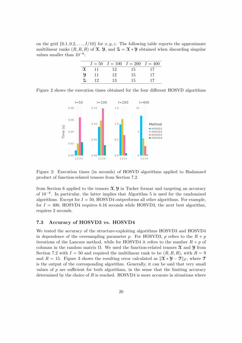
on the grid 0.1, 0.2, . . . , I/10 for x, y, z. The following table reports the approximatemultilinear ranks (R,R,R) of X, Y, and Z = X ∗ Y obtained when discarding singularvalues smaller than 10−8:
I = 50 I = 100 I = 200 I = 400
X 11 12 15 17Y 11 12 15 17Z 12 13 15 17
Figure 2 shows the execution times obtained for the four different HOSVD algorithms
1 2 3 4
HOSVD1HOSVD2HOSVD3HOSVD4
Method
0
5
10
I=400
1 23 40.0
0.5
1.0
1.5
I=200
1 2 3 40.00
0.05
0.10
0.15
I=100
1 2 3 40.00
0.02
0.04
0.06
0.08
Tim
e (
s)
I=50
Figure 2: Execution times (in seconds) of HOSVD algorithms applied to Hadamardproduct of function-related tensors from Section 7.2.
from Section 6 applied to the tensors X,Y in Tucker format and targeting an accuracyof 10−8. In particular, the latter implies that Algorithm 5 is used for the randomizedalgorithms. Except for I = 50, HOSVD4 outperforms all other algorithms. For example,for I = 400, HOSVD4 requires 0.16 seconds while HOSVD3, the next best algorithm,requires 2 seconds.
7.3 Accuracy of HOSVD3 vs. HOSVD4
We tested the accuracy of the structure-exploiting algorithms HOSVD3 and HOSVD4in dependence of the oversampling parameter p. For HOSVD3, p refers to the R + piterations of the Lanczos method, while for HOSVD4 it refers to the number R + p ofcolumns in the random matrix Ω. We used the function-related tensors X and Y fromSection 7.2 with I = 50 and required the multilinear rank to be (R,R,R), with R = 9and R = 15. Figure 3 shows the resulting error calculated as ‖X ∗ Y − T‖F , where T
is the output of the corresponding algorithm. Generally, it can be said that very smallvalues of p are sufficient for both algorithms, in the sense that the limiting accuracydetermined by the choice of R is reached. HOSVD4 is more accurate in situations where
20

the limiting accuracy is below O(10−8), because it works directly with Z(n) instead of
the Gramian Z(n)ZT(n).
HOSVD3HOSVD4
Method
10210
3 43 43 43 4
10-6
10-5
10-4
10-3
10-2
10-1
100
Error
R=9
HOSVD3HOSVD4
Method
10210
3 43 43 43 4
10-15
10-10
10-5
100
Error
R=15
Figure 3: Error of HOSVD3 and HOSVD4 versus oversampling parameter p =0, 2, 4, . . . , 20.
7.4 Execution times for random tensors
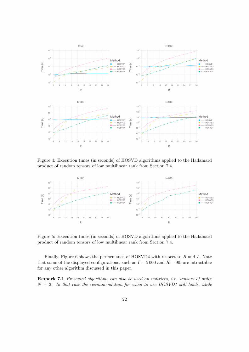
We now choose I × I × I tensors X and Y of prescribed multilinear rank (R,R,R) byletting all coefficients of the Tucker format contain random numbers from the standardnormal distribution. We measure the time needed by our algorithms for truncatingZ = X ∗ Y back to multilinear rank (R,R,R).
Precisely, we use Algorithm 4 with oversampling parameter p = 10 inside algorithmsHOSVD1, HOSVD2 and HOSVD4 and Algorithm 3 with maxit = R + p, for p = 10, inHOSVD3 algorithm. Choosing different reasonable oversampling parameter (e.g. anyp ≤ 20) does not notably change the execution times.
The times obtained for I = 50, 100, 200, 400 with respect to R are shown in Figure 4.As expected the performance of HOSVD1, based on forming the full tensor Z, dependsonly mildly on R. All other algorithms have a cost that is initially smaller than HOSVD1but grows asR increases. The observed breakeven points match the theoretical breakevenpoints between R = O(I2/5) and R = O(I3/5) quite well. For larger I, it is impossible tostore Z and hence Figure 5 only displays the times of HOSVD2, HOSVD3, and HOSVD4for I = 500, 900. Among these three algorithms, HOSVD4 is nearly always the best.Based on these observations, we conclude the following recommendation:
Use HOSVD1 when Z fits into memory and the involved multilinear ranks areexpected to exceed I3/5.
In all other situations, use HOSVD4.
21
R
2 4 6 8 10 12 14 16 18 20
⸻ HOSVD1––– HOSVD2‐‐‐‐‐‐‐ HOSVD3– ‐ – HOSVD4
Method
10-3
10-2
10-1
100
101
Tim
e (s
)I=50
R
3 6 9 12 15 18 21 24 27 30
⸻ HOSVD1––– HOSVD2‐‐‐‐‐‐‐ HOSVD3– ‐ – HOSVD4
Method
10-3
10-2
10-1
100
101
Tim
e (s
)
I=100
R
4 8 12 16 20 24 28 32 36 40
⸻ HOSVD1––– HOSVD2‐‐‐‐‐‐‐ HOSVD3– ‐ – HOSVD4
Method
10-3
10-2
10-1
100
101
102
Tim
e (s
)
I=200
R
5 10 15 20 25 30 35 40 45 50
⸻ HOSVD1––– HOSVD2‐‐‐‐‐‐‐ HOSVD3– ‐ – HOSVD4
Method
10-3
10-2
10-1
100
101
102
103
Tim
e (s
)
I=400
Figure 4: Execution times (in seconds) of HOSVD algorithms applied to the Hadamardproduct of random tensors of low multilinear rank from Section 7.4.
R
5 10 15 20 25 30 35 40 45 50
––– HOSVD2‐‐‐‐‐‐‐ HOSVD3– ‐ – HOSVD4
Method
10-3
10-2
10-1
100
101
102
103
Tim
e (s
)
I=500
R
10 20 30 40 50 60 70 80 90
––– HOSVD2‐‐‐‐‐‐‐ HOSVD3– ‐ – HOSVD4
Method
10-2
10-1
100
101
102
103
104
Tim
e (s
)
I=900
Figure 5: Execution times (in seconds) of HOSVD algorithms applied to the Hadamardproduct of random tensors of low multilinear rank from Section 7.4.
Finally, Figure 6 shows the performance of HOSVD4 with respect to R and I. Notethat some of the displayed configurations, such as I = 5 000 and R = 90, are intractablefor any other algorithm discussed in this paper.
Remark 7.1 Presented algorithms can also be used on matrices, i.e. tensors of orderN = 2. In that case the recommendation for when to use HOSVD1 still holds, while
22

I
500 1000 1500 2000 2500 3000 3500 4000 4500 5000
– ‐ – HOSVD4
Method
101.1
101.2
101.3
101.4
101.5
101.6
101.7
101.8
101.9
Tim
e (s
)
R=50
R
10 20 30 40 50 60 70 80 90
– ‐ – HOSVD4
Method
10-1
100
101
102
103
Tim
e (s
)
I=5000
Figure 6: Execution times (in seconds) of HOSVD4 applied to the Hadamard productof random tensors of low multilinear rank from Section 7.4.
HOSVD3 algorithm outperforms HOSVD2 algorithm in other situations, as is evidentfrom the complexities.
7.5 Testing complexities
Here we test that the complexities presented in this paper match the actual complexitiesof the algorithms HOSVD1, HOSVD2, HOSVD3 and HOSVD4. Using randomly gener-ated tensors X and Y, as in Section 7.4, of size I× I× I and multilinear ranks (R,R,R),with t(I,R) we denote the time needed by our algorithms to recompress Z = X ∗ Y tomultilinear rank (R,R,R). We measure times for two different pairs (I1, R1) and (I2, R2)and compare the ratio t(I1, R1)/t(I2, R2) with the expected ratio e, which is for eachalgorithm defined as follows:
HOSVD1. Since I3 is the dominating term in the complexity of HOSVD1 algo-rithm, we choose I2 = 2I1 and R1 = R2, so the expected ratio is
e =R1I
31
R2I32=
R1I31
R123I31=
1
23,
HOSVD2. Choosing I2 = 24I1 and R2 = 2R1, we have
e =R4
1I1 +R81
R42I2 +R8
2
=R4
1I1 +R8
24R4124I1 + 28R8
=1
28,
HOSVD3 + Variant A. We use this variant when I < R2 so we have to choose Iand R accordingly. If I2 = 2I1 and R2 = 2R1, then
e =R3
1I21 +R5
1I1 +R61
R32I
22 +R5
2I2 +R62
=R3
1I21 +R5
1I1 +R61
23R3122I21 + 25R5
12I1 + 26R61
≈ 1
26,
HOSVD3 + Variant B. We use this variant when I ≥ R2 so we have to choose Iand R accordingly. If I2 = 2I1 and R2 = 2R1, then
e =R5
1I1 +R61
R52I2 +R6
2
=R5
1I1 +R6
25R512I1 + 26R6
=1
26,
23

I1 I2 R1 R2 t(I1, R1)/t(I2, R2) e
HOSVD1 200 400 20 20 0.11615999 0.125HOSVD2 50 800 10 20 0.00225188 0.00390625HOSVD3 + Var. A 200 400 20 40 0.06338479 0.015625HOSVD3 + Var. B 400 800 10 20 0.06642512 0.015625HOSVD4 100 800 20 40 0.02764474 0.015625
Table 1: Comparison of ratios t(I1, R1)/t(I2, R2) and expected ratios e for algorithmsHOSVD1, HOSVD2, HOSVD3 and HOSVD4.
HOSVD4. Choosing I2 = 23I1 and R2 = 2R1, we have
e =R3
1I1 +R61
R32I2 +R6
2
=R3
1I1 +R6
23R3123I1 + 26R6
=1
26,
The results are presented in Table 1.
8 Conclusions
Exploiting structure significantly reduces the computational effort for recompressing theHadamard product of two tensors in the Tucker format. Among the algorithms discussedin this paper, HOSVD4 clearly stands out. It uses a randomized algorithm that employsrandom vectors with rank-1 structure for approximating the range of the matricizations.The analysis of this randomized algorithm is subject to further work. It is not unlikelythat the ideas of HOSVD4 extend to other SVD-based low-rank tensor formats, such asthe tensor train format [22] and hierarchical Tucker format [12].
We view the algorithms presented in this work as a complement to existing toolsfor recompressing tensors. Apart from the HOSVD, other existing tools include thesequentially truncated HOSVD [29], alternating optimization such as HOOI [27], crossapproximation [25], and a Jacobi method [15]. As far as we know, none of these tech-niques has been tailored to the recompression of Hadamard products.
Acknowledgments. The authors thank the referees for helpful remarks on an earlierversion that improved the manuscript and Ivan Slapnicar for helpful discussions.
A Julia package
We have created a Julia [3] package for tensors in Tucker format in programming languageJulia, following the nomenclature of Matlab’s Tensor Toolbox [1]. A notable differenceto the Tensor Toolbox is that we do not construct a separate object tensor for dealingwith full tensors but instead directly use built-in multidimensional arrays. Our packagehas a standard structure:
TensorToolbox.jl/
24

src/
Tensortoolbox.jl
tensor.jl
ttensor.jl
helper.jl
test/
create test data.jl
paperTests.jl
runtests.jl
test data func.jld
The module TensorToolbox is contained in TensorToolbox.jl, functionality for fulltensors is in tensor.jl, and functionality for tensors in the Tucker format is in ttensor.
jl. The object (or composite type) for tensors in Tucker format is called ttensor andconsists of the fields cten (core tensor), fmat (factor matrices), as well as isorth (flagfor orthonormality of factor matrices).
1 type ttensorT<:Number2 cten::ArrayT3 fmat::ArrayMatrix,14 isorth::Bool5 end
All figures from the paper can be recreated using functions from test/paperTests.jl
file, following instructions in the file.Even though in Section 7 we present numerical results only for N = 3 and tensors of
size I× I× I with multilinear ranks (R,R,R), our package implements these algorithmsfor arbitrary order, different mode sizes and different multilinear ranks.
The following tables summarize the functionality of our package.
Functions for tensors - tensor.jl
hosvd HOSVD.innerprod Inner product of two tensors.krontm Kronecker product of two tensors times matrix (n-mode multiplication).matten Matrix tensorisation - fold matrix into a tensor.mkrontv Multiplication of matricized Kronecker product of two tensors by a vector.mrank Multilinear rank of a tensor.mttkrp Matricized tensor times Khatri-Rao product.nrank n-rank of a tensor.sthosvd Sequentially truncated HOSVD.tenmat Tensor matricization - unfold tensor into matrix.tkron Kronecker product of two tensors.ttm Tensor times matrix (n-mode multiplication).ttt Outer product of two tensors.ttv Tensor times vector (n-mode multiplication).
25

Functions for tensors in Tucker format - ttensor.jl
ttensor Construct Tucker tensor for specified core tensor and factor matrices.randttensor Construct random Tucker tensor.
coresize? Size of the core of ttensor.full Construct full tensor (array) from ttensor.had (.*)? Hadamard product of two ttensor.hadcten? Construct core tensor for Hadamard product of two ttensor with specified
factor matrices.hosvd? HOSVD for ttensor.hosvd1? HOSVD1 - computes Tucker representation of Hadamard product of two
ttensor.hosvd2? HOSVD2 - computes Tucker representation of Hadamard product of two
ttensor.hosvd3? HOSVD3 - computes Tucker representation of Hadamard product of two
ttensor.hosvd4? HOSVD4 - computes Tucker representation of Hadamard product of two
ttensor.innerprod Inner product of two ttensor.isequal (==) True if each component of two ttensor is numerically identical.lanczos? Lanczos algorithm adapted for getting factor matrices in algorithm hosvd3.mhadtv? Matricized Hadamard product of two ttensor multiplied by a vector.minus (-)? Subtraction of two ttensor.mrank? Multilinear rank of a ttensor.msvdvals? Singular values of matricized ttensor.mtimes (*) Scalar multiplication for a ttensor.mttkrp Matricized ttensor times Khatri-Rao product.ndims Number of modes for ttensor.norm Norm of a ttensor.nrank? n-rank of a ttensor.nvecs Compute the leading mode-n vectors for ttensor.permutedims Permute dimensions of ttensor.plus (+)? Addition of two ttensor.randrange? Range approximation using randomized algorithm adapted for Hadamard
product of two ttensor.randsvd? Randomized SVD algorithm adapted for getting factor matrices in algo-
rithm hosvd3.reorth? Reorthogonalization of ttensor. Creates new ttensor.reorth!? Reorthogonalization of ttensor. Overwrites existing ttensor.size Size of a ttensor.tenmat? Unfold tensor into matrix - matricization.ttm Tensor times matrix for ttensor (n-mode multiplication).ttv Tensor times vector for ttensor (n-mode multiplication).
26

uminus (-) Unary minus for ttensor.
Functions denoted by ? are not part of Matlab’s Tensors Toolbox and the functionpermutedims is called permute in MATLAB.
References
[1] Brett W. Bader, Tamara G. Kolda, et al. Matlab tensor toolbox version 2.6. Avail-able online, February 2015.
[2] Jonas Ballani and Daniel Kressner. Matrices with hierarchical low-rank structures.In Exploiting hidden structure in matrix computations: algorithms and applications,volume 2173 of Lecture Notes in Math., pages 161–209. Springer, Cham, 2016.
[3] Jeff Bezanson, Alan Edelman, Stefan Karpinski, and Viral B. Shah. Julia: a freshapproach to numerical computing. SIAM Rev., 59(1):65–98, 2017.
[4] F. Bonizzoni, F. Nobile, and D. Kressner. Tensor train approximation of momentequations for elliptic equations with lognormal coefficient. Comput. Methods Appl.Mech. Engrg., 308:349–376, 2016.
[5] L. De Lathauwer, B. De Moor, and J. Vandewalle. A multilinear singular valuedecomposition. SIAM J. Matrix Anal. Appl., 21(4):1253–1278, 2000.
[6] Sergey Dolgov, Boris N. Khoromskij, Alexander Litvinenko, and Hermann G.Matthies. Polynomial chaos expansion of random coefficients and the solution ofstochastic partial differential equations in the tensor train format. SIAM/ASA J.Uncertain. Quantif., 3(1):1109–1135, 2015.
[7] A. Doostan and G. Iaccarino. A least-squares approximation of partial differentialequations with high-dimensional random inputs. J. Comput. Phys., 228(12):4332–4345, 2009.
[8] M. Espig, W. Hackbusch, A. Litvinenko, H. Matthies, and E. Zander. Efficientanalysis of high dimensional data in tensor formats. In J. Garcke and M. Griebel,editors, Sparse Grids and Applications, volume 88 of Lecture Notes in Computa-tional Science and Engineering, pages 31–56. Springer, 2013.
[9] M. Filipovic and A. Jukic. Tucker factorization with missing data with applicationto low-n-rank tensor completion. Multidimensional Systems and Signal Processing,26(3):677–692, 2013.
[10] Michael Griebel and Helmut Harbrecht. Approximation of bi-variate functions:singular value decomposition versus sparse grids. IMA J. Numer. Anal., 34(1):28–54, 2014.
27

[11] W. Hackbusch. Tensor Spaces and Numerical Tensor Calculus. Springer, Heidel-berg, 2012.
[12] W. Hackbusch and S. Kuhn. A new scheme for the tensor representation. J. FourierAnal. Appl., 15(5):706–722, 2009.
[13] N. Halko, P. G. Martinsson, and J. A. Tropp. Finding structure with randomness:probabilistic algorithms for constructing approximate matrix decompositions. SIAMRev., 53(2):217–288, 2011.
[14] B. Hashemi and N. Trefethen. Chebfun in three dimensions. Technical report, 2016.
[15] Mariya Ishteva, P.-A. Absil, and Paul Van Dooren. Jacobi algorithm for the bestlow multilinear rank approximation of symmetric tensors. SIAM J. Matrix Anal.Appl., 34(2):651–672, 2013.
[16] O. Koch and Ch. Lubich. Dynamical tensor approximation. SIAM J. Matrix Anal.Appl., 31(5):2360–2375, 2010.
[17] T. G. Kolda and B. W. Bader. Tensor decompositions and applications. SIAMReview, 51(3):455–500, 2009.
[18] D. Kressner and C. Tobler. Algorithm 941: htucker—a Matlab toolbox for tensorsin hierarchical tucker format. ACM Trans. Math. Softw., 40(3):22:1–22:22, 2014.
[19] N. Lee and A. Cichocki. Fundamental tensor operations for large-scale data analysisin tensor train formats. arXiv preprint arXiv:1405.7786v2, 2016.
[20] C. Musco and C. Musco. Randomized block Krylov methods for stronger and fasterapproximate singular value decomposition. In Conference on Neural InformationProcessing Systems (NIPS), 2015.
[21] A. Nonnenmacher and Ch. Lubich. Dynamical low-rank approximation: appli-cations and numerical experiments. Mathematics and Computers in Simulation,79(4):1346–1357, 2008.
[22] I. V. Oseledets. Tensor-train decomposition. SIAM J. Sci. Comput., 33(5):2295–2317, 2011.
[23] S. Ragnarsson. Structured tensor computations: Blocking, symmetries and Kro-necker factorizations. PhD thesis, Cornell University, 2012.
[24] S. Ragnarsson and C. F. Van Loan. Block tensor unfoldings. SIAM J. Matrix Anal.Appl., 33(1):149–169, 2012.
[25] M. V. Rakhuba and I. V. Oseledets. Fast multidimensional convolution in low-ranktensor formats via cross approximation. SIAM J. Sci. Comput., 37(2):A565–A582,2015.
28
[26] R. Schneider and A. Uschmajew. Approximation rates for the hierarchical tensorformat in periodic Sobolev spaces. J. Complexity, 30(2):56–71, 2014.
[27] B. N. Sheehan and Y. Saad. Higher order orthogonal iteration of tensors (HOOI) andits relation to PCA and GLRAM. In Proceedings of the 2007 SIAM InternationalConference on Data Mining, pages 355–365, 2007.
[28] H. D. Simon and H. Zha. Low-rank matrix approximation using the Lanczos bidi-agonalization process with applications. SIAM J. Sci. Comput., 21(6):2257–2274,2000.
[29] N. Vannieuwenhoven, R. Vandebril, and K. Meerbergen. A new truncation strat-egy for the higher-order singular value decomposition. SIAM J. Sci. Comput.,34(2):A1027–A1052, 2012.
29