Recognizing Car Fluents from Video

Bo Li1,∗, Tianfu Wu2, Caiming Xiong3,∗ and Song-Chun Zhu2

1Beijing Lab of Intelligent Information Technology, Beijing Institute of Technology2Department of Statistics, University of California, Los Angeles 3Metamind Inc.

boli86@bit.edu.cn, tfwu, sczhu@stat.ucla.edu, cmxiong@metamind.io

AbstractPhysical fluents, a term originally used by Newton [40],

refers to time-varying object states in dynamic scenes. Inthis paper, we are interested in inferring the fluents of ve-hicles from video. For example, a door (hood, trunk) isopen or closed through various actions, light is blinking toturn. Recognizing these fluents has broad applications, yethave received scant attention in the computer vision litera-ture. Car fluent recognition entails a unified framework forcar detection, car part localization and part status recog-nition, which is made difficult by large structural and ap-pearance variations, low resolutions and occlusions. Thispaper learns a spatial-temporal And-Or hierarchical modelto represent car fluents. The learning of this model is for-mulated under the latent structural SVM framework. Sincethere are no publicly related dataset, we collect and anno-tate a car fluent dataset consisting of car videos with diversefluents. In experiments, the proposed method outperformsseveral highly related baseline methods in terms of car flu-ent recognition and car part localization.

1. Introduction1.1. Motivation and Objective

The term of physical fluents is first introduced by New-ton [40] to represent the time-varying statuses of objectstates. In the commonsense literature, it is defined as thespecifically varied object status in a time sequence [39]. Asa typical instance, car fluent recognition has applications invideo surveillance and self-driving. In autonomous driving,car fluents are very important to infer the road conditionsand the intents of other drivers. The left of Fig. 1 showsan example, when seeing the left-front door of a roadsidecar is opening, the autonomous car should slow down, passwith cautions, or be ready to stop. In the freeway context,the autonomous car should give way when the front car isblinking to require a left or right lane change (see the mid-dle figure in Fig. 1). In the parking lot scenario, car part

∗This work was done when Bo Li was a visiting student and CaimingXiong was a Postdoc at UCLA.

Figure 1. Some important applications of car fluent recognition.Best viewed in color and zoom in.

status change indicates info for reasoning about human-carinteractions and surveillance, e.g., a woman is opening cartrunk to pick up stuff (see the right of Fig. 1). In general,fluents recognition is also essential in inferring the minds ofhuman and robotics in Cognition, AI and Robotics.

While there is a vast literature in computer vision on ve-hicle detection and viewpoint estimation [16, 21, 45, 46,63, 43, 25, 35, 12], reasoning about the time-varying statesof objects (i.e., fluents) has been rarely studied. Car fluentsrecognition is a hard and unexplored problem. As illustratedin Fig. 2, car fluents have large structural and appearancevariations, low resolutions, and severe occlusions, whichpresent difficulties at multiple levels. In this paper, we ad-dress the following tasks in a hierarchical spatial-temporalAnd-Or Graph (ST-AOG).

i) Detecting cars with different part statuses and occlu-sions (e.g., in Fig.2 (1.b), the frontal-view jeep with hoodbeing open and persons wandering in the front. In the popu-lar car datasets (such as the PASCAL VOC car dataset [15]and KITTI car dataset [20]), most cars do not have openparts (e.g., open trunk/hood/door) together with car-personocclusions. So, a more expressive model is needed in de-tecting cars in car fluent recognition.

ii) Localizing car parts which have low detectability asindividual parts (e.g., the open hood and trunk in Fig. 2(2.c), the tail lights in the last row of Fig. 2) or even areoccluded (e.g., the trunk in Fig. 2 (2.b)). This situation is

4321

… …

(1.a) (1.b)

(2.a) (2.b) (2.c)

(3.a) (3.b) (3.c)

Figure 2. Illustration of the large structural and appearance varia-tions and heavy occlusions in car fluent recognition. We focus onthe fluents of functional car parts (e.g., doors, trunks, lights) in thispaper. For clarity, we show the cropped single cars only. See Fig.1 and Fig. 5 for the whole context. See text for details.

similar, in spirit, to the well-known challenge of localizinghands/feet in human pose recovery [67]. Temporal contex-tual information is needed to localize those parts, besides aspatial hierarchical car pose model.

iii) Recognizing time-varying car part statuses is a newtask. Unlike object attributes (such as gender and race)which are stable for a long time, the time-varying natureof car fluents presents more ambiguities (e.g., in Fig. 2 (3.a-3.c), the periodical status change of car lights, and its am-biguous appearance and geometric features). Unlike actionrecognition which focuses on humans and does not accountfor the pose and statuses of parts [31, 58], car fluent recog-nition is fine-grained in both spatial and temporal domains.

In this paper, we propose to learn a ST-AOG [71, 21,10, 24] to represent car fluents at semantic part-level. Fig.3 shows a portion of our model, the ST-AOG span in bothspatial and temporal dimensions. In space, it represents thewhole car, semantic parts, part status from top to bottom.In time, it represents the location and status transitions ofthe whole car and car parts from left to right. Given a testvideo, ST-AOG will output frame-level car bounding boxes,semantic part (e.g, door, light) bounding boxes, part statuses(e.g., open/close, turn on/off), and video-level car fluents(e.g., opening trunk, turning left).

Because of the lateral edges in Fig. 3, our proposed ST-AOG is no longer a directed acyclic graph (DAG), thus dy-namic programming (DP) cannot be directly utilized. Tocope with this problem, we incorporate loopy belief propa-gation (LBP) [62] and DP in our inference, and adopt a part-based hidden Markov Model (HMM) in temporal transitionfor each semantic part (see Fig. 4). All the appearance, de-formation and motion parameters in our model are trainedjointly under the latent structural SVM framework.

To train and evaluate the ST-AOG, we collect and anno-tate a car fluent dataset due to the lack of publicly avail-able benchmark (Fig. 5 shows some examples, and detailsof the dataset will be given in Section 6.1). Experimental

results show that our model is capable of jointly recogniz-ing semantic car fluents, part positions, and part status invideo. It outperforms several highly related state-of-the-artbaselines in fluent recognition and part localization (slidingwindow-based). Besides, our model can be directly incor-porated with popular improved dense trajectories (iDT) [59]and C3D features [55] to encodes more general information.

2. Related Work and Our ContributionsWe briefly review the most related topics in 3 streams:Car Detection and View Estimation. In computer

vision and intelligent transportation, there is a consider-able body of work on car detection and view estimation[16, 21, 45, 46, 63, 43, 54, 25, 35, 12]. Though thoseworks have successfully improve the performance on popu-lar benchmarks [15, 20], the output is usually the car bound-ing box and a quantized rough view. Some other works[53, 72, 65] aim to get car configurations with detailed orfine-grained output to describe the more meaningful carshape, rather than a bounding box. However, all of thoseworks generally regarded car as a static rigid object, whilepay little attention to the functionalities of semantic carparts and the fact that cars presenting large geometry andappearance transformations during car fluents change.

Video-based Tasks in Vision, Cognition, AI andRobotics. In computer vision, a significant effort has beendevoted to video-based tasks: event [38, 28, 64], actiondetection/recognition [61, 73, 60, 41] and pose estimation[67, 1, 18]. These papers are related to our work, however,most of them are based on human models, while very lit-tle work has done on car fluents and related car part sta-tus estimation. In cognitive science, the concept of fluentsis mainly used to represent the object status changing intime series [39], and it has been used in causality infer-ence [39, 26, 7, 19]. Furthermore, fluents are also relatedto action-planning in AI and Robotics [5, 66].

Human-Object Recognition. As mentioned in [19], thestatus of object fluent change is caused by some other ob-jects. In our case, the car fluent change is mainly conductedby humans. Thus our work is related to part recognition[49, 34] and human-object interactions [50, 33, 23, 68, 6,51, 14]. But, here we jointly and explicitly model car detec-tion, part localization and status estimation.

Our Contributions. This paper makes three contributionsto car fluent recognition:

i) It presents a ST-AOG to represent the spatial-temporalcontext in car fluent recognition. Car fluent recognition is anew task in the computer vision literature.

ii) It presents a new car fluent dataset with per-frame an-notations of cars, car types, semantic parts, part statuses andviewpoints.

iii) It provides a new method for car fluent recognitionand part status estimation, and outperforms several state-of-the-art baseline methods.

4322

Hood

LightHood

LightHood

Light

t

Vie

w B

ran

ches

…

Body Body Body

0

And-node

Or-node

Terminal-node

Motion Flow

Global Motion Flow

Local Motion Flow

Iconic Motion Change

Figure 3. Illustration of the proposed ST-AOG for representing car fluents. In space (vertical), the ST-AOG represents cars by quantizedviews, types, and semantic parts with different statuses. This is used to model appearance and geometry info. In time (horizontal), theST-AOG represents temporal transitions by 3 type of motion flows: Global motion flow, local motion flow and iconic motion change, whichare illustrated on the right. Here, “opn”, “cls”, “occ”, “on”, “off” denotes “open”, “close”, “occluded”, “turn on”, “turn off”, respectively.For each fluent video, our ST-AOG outputs a parse graph consists of frame-level parse trees, which are shown by the bold arrows. We omitthe temporal transitions of Terminal-nodes for clarity.

3. Representation3.1. Spatial-Temporal And-Or Graph

Fig. 3 illustrates our ST-AOG, it models a car fluent bythe viewpoint, car type, semantic parts and correspondingpart statuses hierarchically. In addition to the appearanceand deformation, it also models the temporal transitions ofthe semantic parts.

Utilizing Ii and Ii+1 to denote neighbouring frames, theST-AOG is defined by a 3-tuple,

G = (V,E,Θ) (1)where V is the node set consisting of a set of non-terminal nodes (i.e., And-nodes VAnd and Or-nodes VOr)and a set VT of terminal-nodes (i.e., appearance templates).E = (ES , EM) is the edge set maintaining the struc-ture of the graph. Specifically, ES is the spacial edgesaccounting for composition and deformation, EM is thelateral edges accounting for temporal transitions. Θ =(Θapp,Θdef ,ΘM,Θ

bias) is the set of parameters, and wehave,

i) the appearance parameters Θapp = (Θappt , t ∈ VT )

consists of the appearance templates for all terminal-nodes.Our model is general, in which any type of features can beused. In this paper, we use the histogram of oriented gra-dient (HOG) feature [13] and convolutional neural network(CNN) feature [32] as the appearance feature for illustra-tion.

ii) the deformation parameters Θdef are defined for allin-edges of all terminal-nodes, (v, t) ∈ E (v ∈ VAnd ∪ VOr

and t ∈ VT ), to capture the local deformation when plac-ing a terminal-node t in a feature pyramid. For the defor-mation feature, we adopt the standard separable quadraticfunction of the displacement of t with respect to its parent

node v, (dx, dx2, dy, dy2), as done in the deformable part-based models [16, 2] and the car AOG model [37].

iii) the transition parameters ΘM are defined on the sin-gle car and semantic part nodes. They are used to weightthe effects of temporal transition between Ii and Ii+1. Asillustrated on the right of Fig. 3, we compute 3 types ofmotion flows for car fluents:

a) global motion flow. We compute the optical flow ofthe whole car (e.g., body), and utilize it as the global featureto localize car in time. This global feature is very helpfulfor moving cars, especially in the far view, in which thesemantic part is too small to be detected.

b) local motion flow. We compute the optical flow of“mobile” car part (e.g., door), and utilize it as the temporalfeature to recognize the position and status of the part. Here,the “mobile” car part is the part that can be open or closed,which has motion features during fluent change.

c) iconic motion flow. For car lights, the most distinc-tive feature is its intensity change and temporally periodicalturn on/off statuses. This is related to the work in iconicchange [3, 4] and change detection [47]. Here, we use theappearance and optical flow templates to localize car lights,and compute the temporal intensities (vector of normalizedintensities) to recognize the periodical light status change(e.g., left-turn/right turn).

For optical flow, we compute the pyramid feature to copewith different scales.

iv) the bias parameters Θbias are defined for the childnodes of all Or-nodes to encode either the prior (e.g., differ-ent appearance templates for the “open” part), or the com-patibility of parsing scores among different sub-categories(e.g., different viewpoints of a jeep).

4323

Although the hierarchical structure of our ST-AOG issimilar to those spatial-only models used in [37, 46] for cardetection, we introduce the semantic part Or-nodes (to beused to define fluent) for detailed part status modelling inboth spatial and temporal domains.

A parse tree, pt, is an instantiation of the ST-AOG be-ing placed at a location in the spatial-temporal feature pyra-mid. It is computed by following the breadth-first-searchorder of the nodes in G, selecting the best child node at eachencountered Or-node (based on the scoring function to bedefined later on). The bold black edges in Fig. 3 show theparse trees of ST-AOG on three neighbouring video frames.For a video with N frames, we can get its parse graph aspg = pti,i+1N−1i=1 .

Based on the pg, we extract frame-level part bound-ing boxes and statues, and utilize them to design spatial-temporal features for fluent recognition. To capture long-term spatial-temporal info, our model can also integrate iDT[59] and C3D features [55] (see Section 6.2).

3.2. The Scoring FunctionThe scoring function of ST-AOG is recursively defined

w.r.t. its structure. For simplicity, we will use v and v(v ∈ V ) to represent the temporally neighbouring nodes(on frames Ii and Ii+1) below.

Let O ∈ VOr denotes the Or-node in the ST-AOG, A ∈VAnd be the parent node of a terminal-node t ∈ VT . Wemodel t by a 4-tuple (θappt , θdeft|A , σt, at|A) where σt is thescale factor for placing t w.r.t. A in the feature pyramid(σt ∈ 0, 1), and at|A is the anchor position of t relative toA.

i) Given A, t and their locations lA, lt, the scoring func-tion of placing t at the position lt is then defined by,

S(t|lt, A, lA) = maxlt

[< θappt ,Φapp(lt) > −

< θdeft|A ,Φdef (lt, lA) > +θTM‖lt − lt + F(lt)‖22] (2)

where Φapp(lt) is the appearance features (HOG or CNN)and Φdef (lt, lA) is the deformation features. θTM is the mo-tion flow weight of t. F(l) is the motion flow betweenframes Ii and Ii+1 computed at position l.

ii) Given A and its location lA at frame Ii+1, the scoringfunction of A is defined by,

S(A, lA|A, lA) =∑

v∈ch(A)

[S(v|A, lA) + bA

+ θAM‖lv|A − lv|A + F(lv|A)‖22] (3)

where ch(A) is the set of child nodes of A, bA is the biasparameter. θAM is the motion flow weight of A.

iii) Given O and its location lO at frame Ii+1, the scoringfunction of O is defined by,

S(O, lO|O, lO) = maxv∈ch(O)

[S(v|O, lO)+

θOM‖lv|O − lv|O + F(lv|O)‖22] (4)

where ch(O) is the set of child nodes ofO, lO is the positionof O. θOM is the optical flow weight of O.

For temporal term ‖lv− lv +F(lv)‖22, v ∈ V , since thescoring function of v is conditioned on v in time, while v isconditioned on its child nodes or parent node in space, thereare loops in this structure, and we couldn’t use DP to com-pute above scoring functions directly. As similar to [11], weresort to LBP [62] to get an approximate solution. For com-putational efficiency, the motion flows are computed onlyat nodes corresponds to the car and its semantic parts. Forother nodes, their motion flow are implicitly embedded, astheir score maps are related to nodes with temporal links,and their scoring functions are computed as above but with-out the temporal terms.

Given a fluent video clip withN frames, the overall scoreof ST-AOG will be:

S(I1:N |pg,G) =1

N − 1

N−1∑i=1

Si,i+1(O, lO|O, lO) (5)

where O is the root Or-node in ST-AOG. In probabilisticmodel, Eqn. (5) can be interpreted as a log-posterior prob-ability up to a constant. Our objective is to maximize Eqn.(5), given all appearance, deformation, and motion featuresfrom training videos.

4. Inference by LBP and DPTo cope with the loop introduced by motion transi-

tion, we extend the traditional inference procedure in AOG[37, 69] with LBP. Given an input video, Our inference pro-cedure includes 4 steps:

i) For each frame Ii, we omit the temporal links betweenit and its neighbour frames, and compute the appearancefeature pyramid, optical flow pyramid, and score maps forall nodes in Layer 3− 6 in the ST-AOG by the Depth-First-Search (DFS) order; This step is similar to the inferencealgorithm in [37].

ii) After we get the score maps of the semantic part Or-nodes and the single car And-nodes, we further integrate thescore maps with optical flow maps, as can be seen on the leftof Fig. 4. For each semantic part p with its parent root noder, we focus on four nodes, i.e., p, r, p, r, and omit otherspatial links connected to them. At the beginning, we sendmessage from p to r, then from r to the rest to update themessage. When the difference of the propagated messagein two consecutive iterations doesn’t change, we computethe last “belief” that transmitted to r as r′s score map. Thisprocedure can be efficiently implemented by distance trans-form [17].

iii) After we get the score maps from ii), we further com-pute the score maps for nodes in the upper layers of ST-AOG. By this procedure, the score map of the root Or-nodefor neighbouring frames Ii and Ii+1 can be computed bymaximizing Eqn. (4) on each spatial-temporal point.

4324

Hood

Single

Car

Hood

t t+1

Single

Car

Integrating Optical Flow by LBP

Figure 4. Left: Computing optical flow with LBP. For simplicity,we just show the flow circle of “Body-Hood”. Right: Semanticpart inference with part-based HMM. Here, each bold line repre-sents a frame, circles represent part proposals with different status,thin lines represent the temporal transitions, and semantic parts arerepresented by different colors. For simplicity, we just show thebounding box proposals of the left-front door and left-back door.Best viewed in color and zoom in.

iv) For each spatial-temporal sliding window with scorebeing greater than the threshold τ , we follow the Breadth-First-Search (BFS) order to retrieve its parse tree (includingthe whole car windows, semantic part windows and part sta-tuses at each frame) by taking argmax at each encounteredOr-node.4.1. Post-Refinement

As analysed in [44], we can get more accurate part local-izations by generating multiple object instances in an image.In this paper, we utilize a similar method to generate mul-tiple car part proposals: First of all, we set low detectionthreshold to generate multiple car proposals around the tar-get car, then we execute a conservative non-maximum sup-pression (NMS) procedure to override the observation termand select windows that are not local maxima. By backtrac-ing the parse tree pt, we can get the semantic part proposalsfrom each car proposal.

The right of Fig. 4 illustrates our part-based HMM infer-ence method. For a semantic part p, we can write its bound-ing box sequence in a given video (N frames) as a stochasticset Ωp = piN−1i=1 , then the overall linking scores of part pin a video can be computed as:

S(Ωp) =

N−1∑i=1

S(pi) + θpMψ(pi,i+1) + λov(pi, pi+1) (6)

S(pi) = θpφp(Ii) + θpφp(Ii+1), ψ(pi,i+1) = (dx, dx2, dy, dy2, ds, ds2)

where we model S(pi) as the appearance and deformationscore, θp and φp are the corresponding parameter and fea-ture, θpM is the temporal weights, ψ is the temporal feature,dx, dy, ds are the differences of temporal position and scaleof part p between Ii and Ii+1, ov(pi, pi+1) is the boundingbox overlap of p between Ii and Ii+1. For each semanticpart in the video, we seek the optimal path Ω∗p by maximiz-ing Eqn. (6).

5. Learning by Latent Structural SVMThe training data. In our car fluent dataset, for each

video Xv, v ∈ 1, · · · ,W, we have its annotated parse

graph pg(Xv) including the car bounding boxes, view-points, car types, semantic part bounding boxes, part sta-tuses and corresponding fluent labels.

For parameter optimization, the objective function of ST-AOG is:

minΘ,ξ

E(Θ) =1

2‖Θ‖2 + C

W∑v=1

ξv (7)

s.t. ξv > 0; ∀v, pg(Xv) 6= pg(Xv),

S(pg(Xv))− S(pg(Xv)) ≥ L(pg(Xv), pg(Xv))− ξv

where C is the regularization parameter, pg is the pre-dicted parse graph, and L(pg(Xv), pg(Xv)) is the surro-gate loss function. To accurately predict the viewpoint, cartype, part bounding boxes and part statuses, we specifyL(pg(Xv), pg(Xv)) = 1

vN

∑vNj=1 `(pt(X

jv), pt(Xj

v)) (vNis the number of frames in Xv), and define `(pt, pt) by,

`(pt, pt) =

1 if view or car type is different1 if overlap(pt, pt) < ov

1 if ∃p, pt.status(p) 6= pt.satus(p)0 otherwise

, (8)

where the second term computes the overlap betweentwo parse trees (they have the similar structure, other-wise the loss is computed based on the first term), andoverlap(pt, pt) is defined by the minimum overlap ofbounding boxes of all nodes in the parse trees. The thirdterm check the semantic part status.

The training procedure has the following two steps:i) Initialization. We use standard SVM to train the se-

mantic car part templates on the annotations. For each view,we first cluster the semantic parts by their status, then clus-ter the “open” parts by their aspect ratios, as they have largeappearance and geometry variations. After getting theseclusters, we train a template for each of them. These tem-plates construct the Terminal-nodes in ST-AOG.

ii) Learning the whole ST-AOG under the LSSVM. Asthe groundtruth annotations may not be the most discrim-inative, we allow parts to move around but with a certainoverlap with the groundtruth. Thus the optimization be-comes a latent structural problem. We iterate the followingtwo steps to get a local optima:

Step 1 - Positives Relabelling: Do loss-augmented in-ference for each training video with current model by:

Ω∗p = argmax

P∑p=1

S(Ωp) + L(pg(Xv), pg(Xv)) (9)

Step 2 - Update Weights: With the inferred part bound-ing box and part status sequences, we use standard Struc-tural SVM to optimize the appearance, deformation, andmotion parameters Θ in ST-AOG.

In our implementation, we start with a small number ofnegative examples, and iteratively increase them in the 2nd

step as the iCCCP method [70]. Besides, we also maintaina cache for hard negative mining. Since computing on ev-ery frame is not necessary, we sliding the spatial-temporalwindow by every 3 frames.

4325

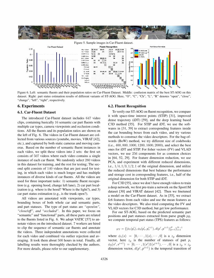
Figure 5. Sample images in Car-Fluent dataset.

Figure 6. Left: semantic fluents and their population ratios on Car-Fluent Dataset. Middle: confusion matrix of the best ST-AOG on thisdataset. Right: part status estimation results of different variants of ST-AOG. Here, “O”, “C”, “Ch”, “L”, “R” denotes “open”, “close”,“change”, “left”, “right”, respectively.

6. Experiments6.1. Car-Fluent Dataset

The introduced Car-Fluent dataset includes 647 videoclips, containing basically 16 semantic car part fluents withmultiple car types, camera viewpoints and occlusion condi-tions. All the fluents and its population ratios are shown onthe left of Fig. 6. The videos in Car-Fluent dataset are col-lected from various sources (youtube, movies, VIRAT [42],etc.), and captured by both static cameras and moving cam-eras. Based on the number of semantic fluent instances ineach video, we split these videos into 2 sets: the first setconsists of 507 videos where each video contains a singleinstance of each car fluent. We randomly select 280 videosin this dataset for training, and the rest for testing; The sec-ond split consists of 140 videos that are just used for test-ing, in which each video is much longer and has multipleinstances of diverse kinds of car fluents. All the videos areused for three important tasks: 1) semantic fluent recogni-tion (e.g. opening hood, change left lane), 2) car part local-ization (e.g. where is the hood? Where is the light?), and 3)car part status estimation (e.g., is the trunk open?).

All videos are annotated with viewpoints, car types,bounding boxes of both whole car and semantic parts,and part statuses. The type of part status are “open/on”,“close/off”, and “occluded”. In this paper, we focus on“semantic” and “functional” parts, all these parts are relatedto the fluents listed in Fig. 6. We adopt VATIC [57] to an-notate videos on the introduced dataset. 7 workers are hiredto clip the sequence of semantic car fluents and annotatethe videos. Three independent annotations were collectedfor each video and combined via outlier rejection and av-eraging. It took them about 500 hours in total. Finally, alllabelling results were thoroughly checked by the authors.For more details, please refer to our supplementary.

6.2. Fluent RecognitionTo verify our ST-AOG on fluent recognition, we compare

it with space-time interest points (STIP) [31], improveddense trajectory (iDT) [59], and the deep learning basedC3D method [55]. For STIP and iDT, we use the soft-wares in [31, 59] to extract corresponding features insidethe car bounding boxes from each video, and try variousmethods to construct the video descriptors. For the bag-of-words (BoW) method, we try different size of codebooks(i.e., 400, 800, 1000, 1200, 1600, 2000), and select the bestones for iDT and STIP. For fisher vectors (FV) and VLADvectors, we use 256 components for as common choicesin [64, 52, 29]. For feature dimension reduction, we usePCA, and experiment with different reduced dimensions,i.e., 1/4, 1/3, 1/2, 1 of the original dimension, and utilizethe reduced dimensions that best balance the performanceand storage cost in corresponding features, i.e., half of theoriginal dimension for both STIP and iDT.

For C3D [55], since we don’t have enough videos to traina deep network, we first pre-train a network on the Sport1Mdataset [30] and VIRAT dataset [42]. Then we finetuneda model on the Car-Fluent dataset. As in [55], we extractfc6 features from each video and use the mean features asthe video descriptors. We also tried computing the FV andVLAD vectors for C3D method, but get low performance.

For our ST-AOG, based on the predicted semantic partpositions and part statuses extracted from parse graph pg,we compute temporal part status (TPS) features as follows:

ϕT = [φ1(pis), φ2(pis, pi+1s ), d(pi, pi+1)]Pp=1N−1

i=1

where φ1(s) = [0, · · · , 1(s), · · · , 0] is a zp dimensionvector, here zp is the number of statuses of part p,φ2(si, si+1) = [0, · · · , 1(si)1(si+1), · · · , 0] is a zp × zpdimension vector, d(pi, pi+1) is the temporal transition of

4326

Figure 7. Examples of part status estimation results on our Car-Fluent dataset. For good visualization, we cropped the cars from originalimages. Different semantic parts are shown by rectangles in different colors (solid for “close/off” status and dashed for “open/on” status).The black lines are used to illustrate variations of the relative positions between whole car and car parts with different statuses. The top 2rows show successful examples. The bottom row shows failure cases, which are mainly caused by occlusion and mis-detected car view.by failure, we mean some part statuses are wrong (e.g., for the 3rd example, the door is correct, but the hood and trunk are wrong). Bestviewed in color and magnification.

BaseLines ST-AOGSTIP-BoW iDT-BoW STIP-FV STIP-VLAD iDT-FV iDT-VLAD C3D TPS TPS+iDT TPS+iDT+C3D

MP 28.8 35.1 35.2 31.5 40.7 41.3 31.0 34.4 45.0 50.8

Table 1. Results of baseline models and our ST-AOG in terms of mean precision (MP) in Car Fluent Recognition.

part p between neighbouring frames. For each car light, wealso compute the mean intensity difference over the lightbounding box across neighbouring frames, and append it toϕT . We compute FV and VLAD vectors on TPS to con-struct the video descriptors as STIP and iDT. For our TPS,we get the best performance with 53 reduced feature dimen-sions for PCA and 256 centers for VLAD vectors.

We use the one-against-rest approach to train multi-classSVM classifiers for above methods. For evaluation, we plotconfusion matrix, and report the mean precision (MP) in flu-ent recognition, equivalent to the average over the diagonalof the confusion matrix.

The first 6 columns in Table 1 show the MP of abovemethods. As can be seen, the “iDT-VLAD” get the bestperformance, while C3D and our TPS get relatively lowerperformances on this dataset, which verified the importanceof motion features. For C3D, we think the relatively lowperformance is due to the lack of training data and it doesn’ttake advantage of car positions. As TPS, iDT and C3D be-long to different type of features, we augment our TPS byintegrating it with iDT and C3D features. To this end, wefirst combine our TPS with iDT, specifically, we try variouscombinations of FV and VLAD vectors, and find the bestone is concatenating TPS VLAD vectors and iDT VLADvectors with square root normalization, as can be seen inTable 1, this improves the performance by about 4; then wefurther combine TPS and iDT VLAD vectors with C3D fea-ture, as can be seen in the last column, we improve the per-formance to 50.8, which outperforms the best single featureby 9.5. From these results we can see, ST-AOG provides

important cues in car fluent recognition, and it’s very gen-eral to integrate with traditional motion features and deeplearning features.

The middle of Fig. 6 shows the confusion matrix ofour “TPS+iDT+C3D” method. We can see the mergedfeature performs pretty well on fluents, i.e., “Open/CloseHood”, “Change Left/Right Lane”, “Left/Right Turn”, buttotally miss fluents, e.g., “Open/Close LB Door”, “CloseRB Door”. For fluents related to the car back door, the lowperformance may be attributed to their ambiguous featuresand relatively low population ratios on current dataset.

6.3. Part Localization and Part Status EstimationSince part location and status are important to fluent

recognition, in this experiment, we further examine theframe-level part localization and status estimation results.

6.3.1 Part LocalizationFor semantic part localization, we use following baselines:(i) Strongly supervised deformable part-based model (SS-DPM) [2]. SSDPM is an open source software, it achievedstate-of-the-art performance on localizing semantic parts ofanimals on PASCAL VOC 2007 dataset [15]. (ii) And-OrStructures [36]. In the literature, [36] also attempted tolocalize the semantic parts by replacing the latent ones inDPM. (iii) Deep DPM (DP-DPM) [22]. The authors in[22] argued that by replacing HOG features with Deep CNNfeatures can improve the detection performance of originalDPM [16]. We use the same trick as [36] to add seman-tic parts on DP-DPM. We also try to compare our modelwith [67, 27, 8, 9], but find it’s hard to compare with them,

4327

SSDPM [2] AOG-Car [36] DP-DPM [22] ST-AOG-HOG ST-AOG-HOG-CSC ST-AOG-CNNBody 96.4 99.1 93.4 99.0 90.8 94.7

Left-front door 36.3 36.6 14.4 49.9 48.0 36.6Left-back door 42.2 44.4 7.1 60.3 55.1 32.3

Right-front door 31.6 40.7 13.0 58.4 55.9 26.8Right-back door 33.0 19.4 14.2 61.4 55.3 32.8

Hood 35.9 20.1 7.1 73.7 67.5 38.4Trunk 25.4 16.8 10.1 54.0 49.7 33.7

Left-head Light 10.4 22.1 19.6 33.1 27.8 29.3Right-head Light 13.3 24.3 15.7 41.3 36.5 23.3

Left-tail Light 6.8 25.7 18.3 27.8 27.3 22.7Right-tail Light 6.2 31.1 14.0 23.2 22.9 14.0

Mean 24.1 28.1 13.4 48.3 44.6 29.0

Table 2. Semantic Car Part Localization results of baseline methods and ST-AOG on Car-Fluent dataset.

as either the code is not available, or the design of parts isinappropriate in our case (details are in the supplementary).

For our ST-AOG, we use several variants for comparison.1)“ST-AOG-HOG” is the instance of our ST-AOG based onHOG features. 2) “ST-AOG-HOG-CSC” is the cascade ver-sion of our model. To improve the speed, we use the re-cently developed Faster-RCNN [48] for cascade detectionof cars. Then based on these car detections, we further runthe ST-AOG for part localization. 3) “ST-AOG-CNN” is theinstance of our ST-AOG based on the pyramid of CNN fea-tures, here, we use the max5 layer of the CNN architecturefor comparison as [22]. To cope with small cars, we doublethe size of source images for CNN.

For evaluation, we compute the detection rate of the se-mantic parts (e.g., “left-front door”, “hood”). Here, we as-sume the whole car bounding boxes are given, and eachmethod only outputs 1 prediction with the highest confi-dence for each groundtruth car. Table 2 shows the quan-titative results. We can see on almost all semantic parts, ourmodel outperforms baseline models by a large margin. Webelieve this is because ST-AOG jointly model the view, partocclusion, geometry and appearance variation, and tempo-ral shifts. For “ST-AOG-HOG-CSC”, we just use it as areference to improve the speed of ST-AOG, since it has thenearly real-time speed, and can be plugged in our modelas an outlier-rejection module. Surprisingly, CNN fea-tures perform worse than HOG features on the Car-Fluentsdataset. In experiments, we find the extracted CNN fea-ture on deep pyramid [22] is too coarse (the cell size is 16),even we resize original images by 2 times, it still miss manysmall parts. Based on recent study of using CNN for key-points prediction [56], we believe a more effective methodis required to integrate CNN feature with graphical models.

6.3.2 Part Status Estimation

To the best of our knowledge, no model tried to output carpart status in our case in the literature. To evaluate the partstatus, we compare different versions of our model and anal-yse the effects of different components. Specifically, wecompute the part status detection rates, that is, a part statusis correct if and only if its position and status (e.g., open,close) are both correct.

On the right of Fig. 6, we show the quantitative results of

4 versions of our ST-AOG. Here, we use HOG features forsimplicity. “ST-AOG-ver1” refers to the ST-AOG withoutboth view and part status penalty in Eqn. (8), “ST-AOG-ver2” refers to the ST-AOG without view penalty in Eqn.(8), and “ST-AOG” is the full model with all penalty in Eqn.(8). To investigate the effect of motion flow, we also com-pare the ST-AOG without motion flow, i.e., the “S-AOG”.As can be seen, the view penalty is the most important fac-tor, then is the part status and motion flow, and part sta-tus seems to have more importance. Interestingly, for someparts (e.g., “RB-Door”), adding more penalty or temporalinfo will decrease the performance.

Fig. 7 shows some qualitative running examples of ST-AOG. The first two rows show the successful results, the lastrow shows the failure examples. For better visualization, wecropped the image to just contain the interested car. We cansee our model can localize parts and recognize their statusesfairly good with different viewpoints and car types, but mayreport wrong results when people occlude the car, the view-points are mis-detected, or there are background clutters.

7. ConclusionThis paper proposed a ST-AOG to recognize car flu-

ents at semantic part-level from video. The ST-AOG inte-grates the motion features in temporal, and a LBP-based DPmethod can be used in inference. The model parameters arelearned under the latent structural SVM (LSSVM) frame-work. To promote the research of fluents, we have collecteda new Car-Fluent dataset with detailed annotations of view-points, car types, part bounding boxes, and part statuses.This dataset presents new challenges to computer vision,and complements existing benchmarks. Our experimentsverified the ability of proposed ST-AOG on fluent recogni-tion, part localization, and part status estimation.

In future work, we will integrate human and car jointly,and study human-car interactions to help understand humanactions/intents based on car fluent recognition.Acknowledgement: B. Li is supported by China 973 Pro-gram under Grant NO. 2012CB316300. T.F. Wu and S.C.Zhu are supported by DARPA SIMPLEX Award N66001-15-C-4035, ONR MURI project N00014-16-1-2007, andNSF IIS 1423305. We thank Tianming Shu, Xiaohan Nieand Dan Xie for helpful discussions.

4328

References[1] M. Andriluka, S. Roth, and B. Schiele. Pictorial structures

revisited: People detection and articulated pose estimation.In CVPR, 2009.

[2] H. Azizpour and I. Laptev. Object detection using strongly-supervised deformable part models. In ECCV, 2012.

[3] M. J. Black, D. J. Fleet, and Y. Yacoob. A framework formodeling appearance change in image sequences. In ICCV,pages 660–667, 1998.

[4] M. J. Black, D. J. Fleet, and Y. Yacoob. Robustly estimatingchanges in image appearance. Computer Vision and ImageUnderstanding, 78(1):8 – 31, 2000.

[5] A. Blum and M. L. Furst. Fast planning through planninggraph analysis. In IJCAI, 1995.

[6] L. Bourdev and J. Malik. Poselets: Body part detectorstrained using 3d human pose annotations. In ICCV, 2009.

[7] M. Brand. The ”inverse hollywood problem”: From videoto scripts and storyboards via causal analysis. In In Proceed-ings, AAAI97, 1997.

[8] X. Chen, R. Mottaghi, X. Liu, S. Fidler, R. Urtasun, andA. Yuille. Detect what you can: Detecting and representingobjects using holistic models and body parts. In CVPR, 2014.

[9] X. Chen and A. Yuille. Articulated pose estimation by agraphical model with image dependent pairwise relations. InNIPS, 2014.

[10] Y. Chen, L. Zhu, C. Lin, A. L. Yuille, and H. Zhang. Rapidinference on a novel and/or graph for object detection, seg-mentation and parsing. In NIPS, 2007.

[11] A. Cherian, J. Mairal, K. Alahari, and C. Schmid. Mixingbody-part sequences for human pose estimation. In CVPR,2014.

[12] J.-Y. Choi, K.-S. Sung, and Y.-K. Yang. Multiple Vehi-cles Detection and Tracking based on Scale-Invariant FeatureTransform. In ITSC, 2007.

[13] N. Dalal and B. Triggs. Histograms of oriented gradients forhuman detection. In CVPR, 2005.

[14] C. Desai and D. Ramanan. Detecting actions, poses, andobjects with relational phraselets. In ECCV, 2012.

[15] M. Everingham, L. Van Gool, C. Williams, J. Winn, andA. Zisserman. The pascal visual object classes (voc) chal-lenge. IJCV, 2010.

[16] P. Felzenszwalb, R. Girshick, D. McAllester, and D. Ra-manan. Object detection with discriminatively trained part-based models. PAMI, 2010.

[17] P. F. Felzenszwalb and D. P. Huttenlocher. Distance trans-forms of sampled functions. Theory of Computing, 2012.

[18] V. Ferrari, M. Marin-Jimenez, and A. Zisserman. Posesearch: Retrieving people using their pose. In CVPR, 2009.

[19] A. Fire and S.-C. Zhu. Using causal induction in humans tolearn and infer causality from video. In CogSci, 2013.

[20] A. Geiger, P. Lenz, and R. Urtasun. Are we ready for au-tonomous driving? the kitti vision benchmark suite. InCVPR, 2012.

[21] R. Girshick, P. Felzenszwalb, and D. McAllester. Object de-tection with grammar models. In NIPS, 2011.

[22] R. Girshick, F. Iandola, T. Darrell, and J. Malik. Deformablepart models are convolutional neural networks. In CVPR,2015.

[23] A. Gupta, A. Kembhavi, and L. S. Davis. Observing human-object interactions: Using spatial and functional compatibil-ity for recognition. TPAMI, 2009.

[24] A. Gupta, P. Srinivasan, J. Shi, and L. S. Davis. Understand-ing videos, constructing plots learning a visually groundedstoryline model from annotated videos. In CVPR, 2009.

[25] K. He, L. Sigal, and S. Sclaroff. Parameterizing object de-tectors in the continuous pose space. In ECCV, 2014.

[26] D. Heckerman. A bayesian approach to learning causal net-works. In Proceedings of the Eleventh Conference on Uncer-tainty in Artificial Intelligence, 1995.

[27] M. Hejrati and D. Ramanan. Analyzing 3d objects in clut-tered images. In NIPS, 2012.

[28] S. Hongeng, R. Nevatia, and F. Brmond. Video-based eventrecognition: activity representation and probabilistic recog-nition methods. Computer Vision and Image Understanding,96(2):129–162, 2004.

[29] H. Jegou, M. Douze, C. Schmid, and P. Perez. Aggregatinglocal descriptors into a compact image representation. InCVPR, 2010.

[30] A. Karpathy, G. Toderici, S. Shetty, T. Leung, R. Sukthankar,and L. Fei-Fei. Large-scale video classification with convo-lutional neural networks. In CVPR, 2014.

[31] I. Laptev, M. Marszałek, C. Schmid, and B. Rozenfeld.Learning realistic human actions from movies. In CVPR,2008.

[32] Y. LeCun, B. Boser, J. S. Denker, D. Henderson, R. E.Howard, W. Hubbard, and L. D. Jackel. Backpropagationapplied to handwritten zip code recognition. Neural Compu-tation, 1:541–551, 1989.

[33] J. T. Lee, M. S. Ryoo, and J. K. Aggarwal. View independentrecognition of human-vehicle interactions using 3-d models.In WMVC, 2009.

[34] T. S. H. Lee, S. Fidler, and S. Dickinson. Detecting curvedsymmetric parts using a deformable disc model. In ICCV,2013.

[35] M. J. Leotta and J. L. Mundy. Vehicle Surveillance with aGeneric, Adaptive, 3D Vehicle Model. TPAMI, 2011.

[36] B. Li, W. Hu, T.-F. Wu, and S.-C. Zhu. Modeling occlusionby discriminative and-or structures. In ICCV, 2013.

[37] B. Li, T. Wu, and S.-C. Zhu. Integrating context and oc-clusion for car detection by hierarchical and-or model. InECCV, 2014.

[38] L.-J. Li and F.-F. Li. What, where and who? classifyingevents by scene and object recognition. In ICCV, 2007.

[39] E. T. Mueller. Commonsense Reasoning. Morgan Kaufmann,San Francisco, 2006.

[40] I. Newton and J. Colson. The Method of Fluxions And InfiniteSeries: With Its Application to the Geometry of Curve-Lines.Nourse, 1736.

[41] B. X. Nie, C. Xiong, and S.-C. Zhu. Joint action recognitionand pose estimation from video. In CVPR, 2015.

[42] S. Oh, A. Hoogs, A. Perera, N. Cuntoor, C.-C. Chen, J. T.Lee, S. Mukherjee, J. K. Aggarwal, H. Lee, L. Davis,

4329

E. Swears, X. Wang, Q. Ji, K. Reddy, M. Shah, C. Vondrick,H. Pirsiavash, D. Ramanan, J. Yuen, A. Torralba, B. Song,A. Fong, A. Roy-Chowdhury, and M. Desai. A large-scale benchmark dataset for event recognition in surveillancevideo. In CVPR, 2011.

[43] E. Ohn-Bar and M. Trivedi. Learning to detect vehicles byclustering appearance patterns. TITS, 2015.

[44] D. Park and D. Ramanan. N-best maximal decoders for partmodels. In ICCV. IEEE, 2011.

[45] B. Pepik, M. Stark, P. Gehler, and B. Schiele. Teaching 3dgeometry to deformable part models. In CVPR, 2012.

[46] B. Pepik, M. Stark, P. Gehler, and B. Schiele. Occlusionpatterns for object class detection. In CVPR, 2013.

[47] R. J. Radke, S. Andra, O. Al-Kofahi, and B. Roysam. Imagechange detection algorithms: A systematic survey. Trans.Img. Proc., 14(3):294–307, Mar. 2005.

[48] S. Ren, K. He, R. Girshick, and J. Sun. Faster R-CNN:Towards Real-Time Object Detection with Region ProposalNetworks. In NIPS, 2015.

[49] E. Rivlin, S. J. Dickinson, and A. Rosenfeld. Recognition byfunctional parts. In CVPR, 1994.

[50] M. S. Ryoo, J. T. Lee, and J. K. Aggarwal. Video sceneanalysis of interactions between humans and vehicles usingevent context. In CIVR. ACM, 2010.

[51] M. A. Sadeghi and A. Farhadi. Recognition using visualphrases. In CVPR, 2011.

[52] J. Sanchez, F. Perronnin, T. Mensink, and J. Verbeek. Im-age classification with the fisher vector: Theory and practice.IJCV, 2013.

[53] M. Stark, J. Krause, B. Pepik, D. Meger, J. J. Little,B. Schiele, and D. Koller. Fine-grained categorization for3d scene understanding. In BMVC, 2012.

[54] J. Tao, M. Enzweiler, U. Franke, D. Pfeiffer, and R. Klette.What is in front? multiple-object detection and tracking withdynamic occlusion handling. In G. Azzopardi and N. Petkov,editors, CAIP, 2015.

[55] D. Tran, L. Bourdev, R. Fergus, L. Torresani, and M. Paluri.Learning spatiotemporal features with 3d convolutional net-works. In ICCV. IEEE, 2015.

[56] S. Tulsiani and J. Malik. Viewpoints and keypoints. InCVPR, 2015.

[57] C. Vondrick, D. Patterson, and D. Ramanan. Efficiently scal-ing up crowdsourced video annotation. IJCV, 2013.

[58] H. Wang, A. Klaser, C. Schmid, and C.-L. Liu. ActionRecognition by Dense Trajectories. In CVPR, 2011.

[59] H. Wang and C. Schmid. Action recognition with improvedtrajectories. In ICCV, 2013.

[60] J. Wang and Y. Wu. Learning maximum margin temporalwarping for action recognition. In ICCV, 2013.

[61] D. Weinland, R. Ronfard, and E. Boyer. A survey of vision-based methods for action representation, segmentation andrecognition. Computer Vision and Image Understanding,115(2):224–241, 2011.

[62] Y. Weiss. Correctness of local probability propagation ingraphical models with loops, 2000.

[63] Y. Xiang, W. Choi, Y. Lin, and S. Savarese. Data-driven3d voxel patterns for object category recognition. In CVPR,2015.

[64] Z. Xu, Y. Yang, and A. G. Hauptmann. A discriminative cnnvideo representation for event detection. In CVPR, 2015.

[65] L. Yang, P. Luo, C. C. Loy, and X. Tang. A large-scale cardataset for fine-grained categorization and verification. InCVPR, 2015.

[66] Y. Yang, Y. Li, C. Fermuller, and Y. Aloimonos. Robot learn-ing manipulation action plans by Watching unconstrainedvideos from world wide web. In AAAI 2015, Austin, US,jan 2015.

[67] Y. Yang and D. Ramanan. Articulated pose estimation withflexible mixtures-of-parts. In CVPR, 2011.

[68] B. Yao and L. Fei-Fei. Recognizing human-object interac-tions in still images by modeling the mutual context of ob-jects and human poses. TPAMI, 2012.

[69] J. Zhu, T. Wu, S.-C. Zhu, X. Yang, and W. Zhang. Learningreconfigurable scene representation by tangram model. InWACV, 2012.

[70] L. Zhu, Y. Chen, A. L. Yuille, and W. T. Freeman. Latent hi-erarchical structural learning for object detection. In CVPR,2010.

[71] S.-C. Zhu and D. Mumford. A stochastic grammar of images.Found. Trends. Comput. Graph. Vis., 2006.

[72] M. Z. Zia, M. Stark, and K. Schindler. Explicit OcclusionModeling for 3D Object Class Representations. In CVPR,2013.

[73] S. Zuffi, J. Romero, C. Schmid, and M. J. Black. Estimatinghuman pose with flowing puppets. In ICCV, 2013.

4330