RECOGNITION

Thanks to Svetlana Lazebnik and Andrew Zisserman for the use of some

slides

How many categories?

10,000-30,000

OBJECTS

ANIMALS INANIMATEPLANTS

MAN-MADENATURALVERTEBRATE …..

MAMMALS BIRDS

PIGEONHORSECOW CHAIR

Camera position Illumination Shape parameters

Within-class variations?

Variability makes recognition hard

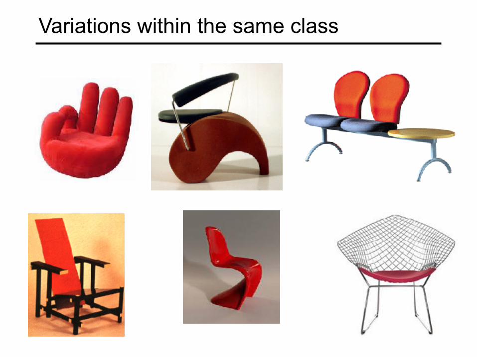
Variations within the same class

History 1960s – early 1990s: geometry 1990s: appearance Mid-1990s: sliding window Late 1990s: local features Early 2000s: parts-and-shape models Mid-2000s: bags of features Present trends: data-driven methods, context

2D objects

Eigenfaces (Turk & Pentland, 1991)

Local features

D. Lowe (1999, 2004)

Image classification

The statistical learning framework

• Apply a prediction function to a feature representation of the image to get the desired output:

f( ) = “apple” f( ) = “tomato” f( ) = “cow”

The statistical learning framework

y = f(x)

• Training: given a training set of labeled examples {(x1,y1), …, (xN,yN)}, estimate the prediction function f by minimizing the prediction error on the training set

• Testing: apply f to a never before seen test example x and output the predicted value y = f(x)

output prediction function

Image feature

Prediction

StepsTraining LabelsTraining

Images

Training

Training

Image Features

Image Features

Testing

Test Image

Learned model

Learned model

Slide credit: D. Hoiem

Traditional recognition pipeline

Hand-designedfeature

extraction

Trainableclassifier

Image Pixels

• Features are not learned • Trainable classifier is often generic (e.g. SVM)

ObjectClass

Bags of features

1. Extract local features 2. Learn “visual vocabulary” 3. Quantize local features using visual vocabulary 4. Represent images by frequencies of “visual words”

Traditional features: Bags-of-features

Texture recognition

Universal texton dictionary

histogram

Julesz, 1981; Cula & Dana, 2001; Leung & Malik 2001; Mori, Belongie & Malik, 2001; Schmid 2001; Varma & Zisserman, 2002, 2003; Lazebnik, Schmid & Ponce, 2003

1. Local feature extraction• Sample patches and extract descriptors

Keypoints

patches surrounding keypoints

2. Learning the visual vocabulary

…

Slide credit: Josef Sivic except for the image patches

Extracted descriptors from the training set

patches surrounding keypoints

2. Learning the visual vocabulary

Clustering

…

Slide credit: Josef Sivic

2. Learning the visual vocabulary

Clustering

…

Slide credit: Josef Sivic

Visual vocabulary

Review: K-means clustering• Want to minimize sum of squared Euclidean

distances between features xi and their nearest cluster centers mk

Algorithm: • Randomly initialize K cluster centers • Iterate until convergence:

• Assign each feature to the nearest center • Recompute each cluster center as the mean of all features

assigned to it

∑ ∑ −=k

ki

kiMXDcluster

clusterinpoint

2)(),( mx

Example visual vocabulary

…

Source: B. Leibe

Appearance codebook

1. Extract local features 2. Learn “visual vocabulary” 3. Quantize local features using visual vocabulary 4. Represent images by frequencies of “visual words”

Bag-of-features steps

• Orderless document representation: frequencies of words from a dictionary Salton & McGill (1983)

Bags of features: Motivation

US Presidential Speeches Tag Cloudhttp://chir.ag/projects/preztags/

• Orderless document representation: frequencies of words from a dictionary Salton & McGill (1983)

Bags of features: Motivation

US Presidential Speeches Tag Cloudhttp://chir.ag/projects/preztags/

• Orderless document representation: frequencies of words from a dictionary Salton & McGill (1983)

Bags of features: Motivation

US Presidential Speeches Tag Cloudhttp://chir.ag/projects/preztags/

• Orderless document representation: frequencies of words from a dictionary Salton & McGill (1983)

Bags of features: Motivation

Spatial pyramids

level 0

Lazebnik, Schmid & Ponce (CVPR 2006)

Spatial pyramids

level 0 level 1

Lazebnik, Schmid & Ponce (CVPR 2006)

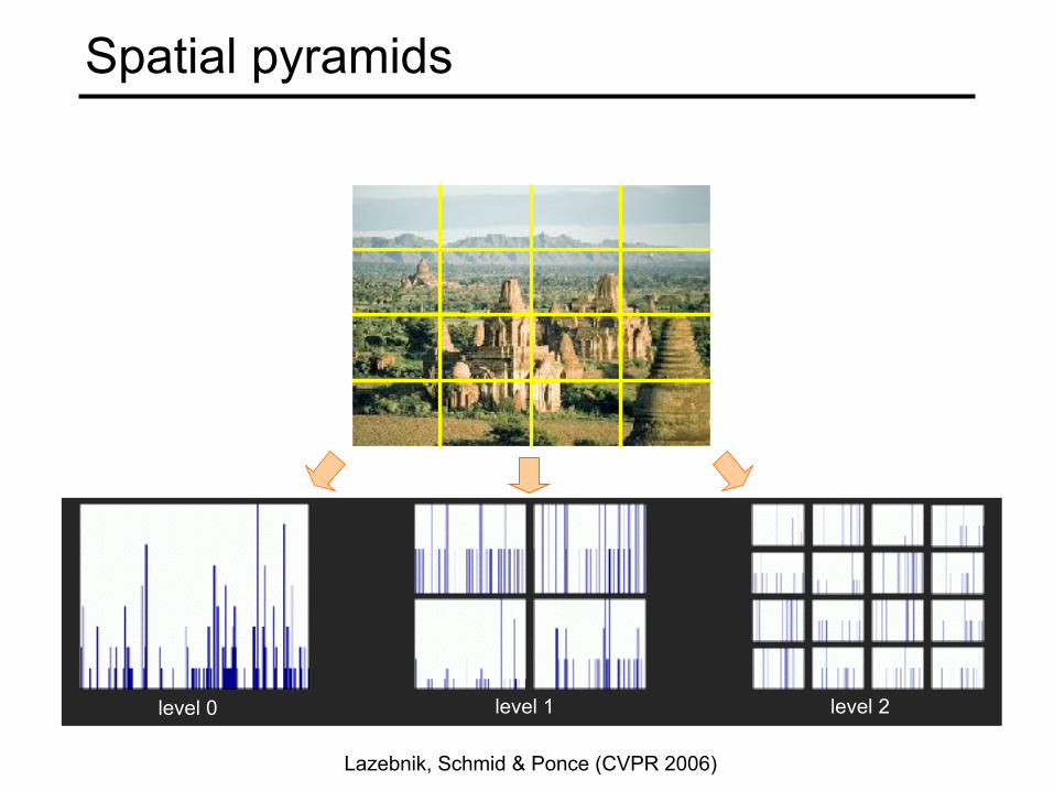
Spatial pyramids

level 0 level 1 level 2

Lazebnik, Schmid & Ponce (CVPR 2006)

Spatial pyramids• Scene classification results

Spatial pyramids• Caltech101 classification results

Traditional recognition pipeline

Hand-designedfeature

extraction

Trainableclassifier

Image Pixels

ObjectClass

Classifiers: Nearest neighbor

f(x) = label of the training example nearest to x

All we need is a distance function for our inputs No training required!

Test example

Training examples

from class 1

Training examples

from class 2

K-nearest neighbor classifier• For a new point, find the k closest points from

training data • Vote for class label with labels of the k points

k = 5

K-nearest neighbor classifier

Which classifier is more robust to outliers?

Credit: Andrej Karpathy, http://cs231n.github.io/classification/

K-nearest neighbor classifier

Credit: Andrej Karpathy, http://cs231n.github.io/classification/

Linear classifiers

Find a linear function to separate the classes:

f(x) = sgn(w ⋅ x + b)

Visualizing linear classifiers

Source: Andrej Karpathy, http://cs231n.github.io/linear-classify/

Nearest neighbor vs. linear classifiers• NN pros:

• Simple to implement • Decision boundaries not necessarily linear • Works for any number of classes • Nonparametric method

• NN cons: • Need good distance function • Slow at test time

• Linear pros: • Low-dimensional parametric representation • Very fast at test time

• Linear cons: • Works for two classes • How to train the linear function? • What if data is not linearly separable?

Support vector machines• When the data is linearly separable, there may

be more than one separator (hyperplane)

Which separatoris best?

Support vector machines• Find hyperplane that maximizes the margin

between the positive and negative examples

1:1)(negative1:1)( positive−≤+⋅−=

≥+⋅=

byby

iii

iii

wxxwxx

MarginSupport vectors

C. Burges, A Tutorial on Support Vector Machines for Pattern Recognition, Data Mining and Knowledge Discovery, 1998

Distance between point and hyperplane: ||||

||wwx bi +⋅

For support vectors, 1±=+⋅ bi wx

Therefore, the margin is 2 / ||w||

Finding the maximum margin hyperplane1. Maximize margin 2 / ||w|| 2. Correctly classify all training data:

Quadratic optimization problem:

C. Burges, A Tutorial on Support Vector Machines for Pattern Recognition, Data Mining and Knowledge Discovery, 1998

1)(subject to21

min 2

,≥+⋅ by iib

xwww

1:1)(negative1:1)( positive−≤+⋅−=

≥+⋅=

byby

iii

iii

wxxwxx

SVM parameter learning

• Separable data:

• Non-separable data:

1)(subject to21

min 2

,≥+⋅ by iib

xwww

Maximize margin Classify training data correctly

minw,b

12w 2

+C max 0,1− yi (w⋅xi +b)( )i=1

n

∑

Maximize margin Minimize classification mistakes

SVM parameter learning

Demo: http://cs.stanford.edu/people/karpathy/svmjs/demo

Margin

+1

-10

minw,b

12w 2

+C max 0,1− yi (w⋅xi +b)( )i=1

n

∑

Nonlinear SVMs• General idea: the original input space can always

be mapped to some higher-dimensional feature space where the training set is separable

Φ: x → φ(x)

Image source

• Linearly separable dataset in 1D:

• Non-separable dataset in 1D:

• We can map the data to a higher-dimensional space:

0 x

0 x

0 x

x2

Nonlinear SVMs

Slide credit: Andrew Moore

The kernel trick• General idea: the original input space can always

be mapped to some higher-dimensional feature space where the training set is separable

• The kernel trick: instead of explicitly computing the lifting transformation φ(x), define a kernel function K such that K(x , y) = φ(x) · φ(y)

(to be valid, the kernel function must satisfy Mercer’s condition)

The kernel trick• Linear SVM decision function:

C. Burges, A Tutorial on Support Vector Machines for Pattern Recognition, Data Mining and Knowledge Discovery, 1998

bybi iii +⋅=+⋅ ∑ xxxw α

Support vector

learnedweight

The kernel trick• Linear SVM decision function:

• Kernel SVM decision function:

• This gives a nonlinear decision boundary in the original feature space

bKybyi

iiii

iii +=+⋅ ∑∑ ),()()( xxxx αϕϕα

C. Burges, A Tutorial on Support Vector Machines for Pattern Recognition, Data Mining and Knowledge Discovery, 1998

bybi iii +⋅=+⋅ ∑ xxxw α

Polynomial kernel: dcK )(),( yxyx ⋅+=

Gaussian kernel• Also known as the radial basis function (RBF)

kernel:

⎟⎠

⎞⎜⎝

⎛ −−=2

2

1exp),( yxyx

σK

||x – y||

K(x, y)

Gaussian kernel

SV’s

Kernels for histograms• Histogram intersection:

• Square root (Bhattacharyya kernel):

K(h1,h2 ) = min(h1(i),h2 (i))i=1

N

∑

K(h1,h2 ) = h1(i)h2 (i)i=1

N

∑

SVMs: Pros and cons• Pros

• Kernel-based framework is very powerful, flexible • Training is convex optimization, globally optimal solution can

be found • Amenable to theoretical analysis • SVMs work very well in practice, even with very small training

sample sizes

• Cons • No “direct” multi-class SVM, must combine two-class SVMs

(e.g., with one-vs-others) • Computation, memory (esp. for nonlinear SVMs)

Generalization• Generalization refers to the ability to correctly

classify never before seen examples • Can be controlled by turning “knobs” that affect

the complexity of the model

Training set (labels known) Test set (labels unknown)

Diagnosing generalization ability• Training error: how does the model perform on the data on

which it was trained? • Test error: how does it perform on never before seen data?

Training error

Test error

Source: D. Hoiem

Underfitting Overfitting

Model complexity HighLow

Err

or

Underfitting and overfitting• Underfitting: training and test error are both high

• Model does an equally poor job on the training and the test set • Either the training procedure is ineffective or the model is too

“simple” to represent the data • Overfitting: Training error is low but test error is high

• Model fits irrelevant characteristics (noise) in the training data • Model is too complex or amount of training data is insufficient

Underfitting OverfittingGood generalization

Figure source

Effect of training set size

Many training examples

Few training examples

Model complexity HighLow

Test

Err

or

Source: D. Hoiem

Validation• Split the data into training, validation, and test subsets • Use training set to optimize model parameters • Use validation test to choose the best model • Use test set only to evaluate performance

Model complexity

Training set loss

Test set loss

Err

or

Validation set loss

Stopping point

SummaryThe different steps