The impact of mining sector on growth, inequality, and

poverty: Evidence from Armenia

Aleksandr Grigoryan∗

April 11, 2013

Abstract

We use regional data for the Armenian economy to estimate the impact of themining sector on growth, income inequality and poverty. Despite a relatively smallshare of mining idustry in GDP, it has an important role in shaping the evolution ofthe industry structure.

The main findings are as follows. An accelerated expansion of the mining sectorenhances growth - a good news for policy makers to justify pro-mining policies. Miningsector, however, is likely to increase income inequality and deepen poverty in Armenia.

We study small sample properties of our estimates by bootstrap analysis. Growthmodels survive the test, but inequality and poverty models fail to report significantcoefficients for mining. Nevertheless, the sign and magnitudes are preserved in mostcases with little drop of P-values. We also check our specifications, excluding one region(Syunik marz), which absorbs a huge share of mining in Armenia. As expected, theexclusion of Syunik marz makes our models less dependent from the mining sector.

Keywords: Armenia, mining, growth, income inequality, poverty.

1 Introduction

In this paper we analyze the impact of the industry structure on growth, inequality and

poverty for the Armenian economy, searching for model specifications in which the mining

sector1 has a significant role. Mining has a small share in GDP and the dynamics is rather

driven by external factors. This motivates to interpret movements in mining share as an

exogenous variation, which may well explain the evolution of GDP growth, income inequality

and poverty measures.

∗American University of Armenia (AUA); e-mail: aleksandr@aua.am. This work was commissioned bythe AUA Acopian Center for the Environment.

1We use the term ”mining” for the sector Mining and quarrying throughout the paper.

1

Over the last two decades Armenia has made substantial steps in liberalizing politico-

economic environment via continuation of reforms, committed at the early stage of inde-

pendence. In particular, the economy has experienced sound economic growth, severely

disrupted by the world financial crisis in 2008. The Armenian authorities have succeeded to

sustain high growth rate and consistently decreasing inequality along this period, with signifi-

cant help of international organizations. Overall, GDP and the two inequality measures (Gini

index and poverty rate) move together, ensuring higher growth and less inequality/poverty

in 2000-2008 (see Figure 1).2 A recent paper by Begrakyan and Grigoryan (2012) analyze

the dynamics of income inequality and poverty for Armenia, using a large set of explanatory

variables.

010

2030

4050

2000 2002 2004 2006 2008year

Poverty headcount ratio at $2 a day Gini coefficientReal GDP growth rate

Figure 1: GDP growth, inequality and poverty for the Armenian economy. Source: NSSRA.

Despite satisfactory aggregate economic indicators, challenges the economy faces in its

transition remain actual. The Armenian economy heavily depends on remittances, which

effectively transfers external shocks to domestic markets. Trade imbalances with the rest of

the world is another channel by which Armenia faces external shocks. High concentration in

domestic markets together with strong dependence of foreign currency inflows sustain foreign

2Recent macroeconomics developments in Armenia is properly documented in, e.g., IMF (2011).

2

exchange risk at a very high level3.

A separate channel the economy depends on the rest of the world, is the export of the

mining product. Intuitively, high prices on ores and metals in world markets should push

local producers to increase extraction of local mines and sales abroad. On the other side,

mining capacities are fixed in the short run and temporary fluctuation of prices need not

align current production volumes4. Overall, the export of mining has decreased at the early

stage of crisis (2008-2009) (Figure 4)5, but its share has even increased in GDP.

Figure 2: Mining’s contrbution to export, GDP and growth

The contributions of mining to the exports, GDP and its growth are crucially different.

Despite its modest share in GDP (it averages to 2 percent in 2000-2010), mining covers almost

20 percent of the total export and its contribution to growth comprises around 10 percent in

2008-2010. Figure 2 reflects these differences. There is also strong correlation between the

mining share in exports and mining’s contribution to GDP growth6. While the very small

share of mining in GDP may undermine its role in explaining the evolution of the industry

3The impact of external imbalances on domestic prices and activity is analyzed by Oomes et al. (2009).4Mining in Armenia seems to be far from its capacity utilization, however, there may be positive cor-

relation between metal prices and the produced volumes in mining. For example, copper prices in worldmarkets and mined volumes in Armenia have dramatically dropped during the crisis time, while the shareof copper mining has increased in that period. Analysis of potential comovements/causalities in prices andmined volumes, interesting in its own, is beyond the scope of this paper.

5Source: Kostanyan (2011)6The correlation coefficient is 0.85.

3

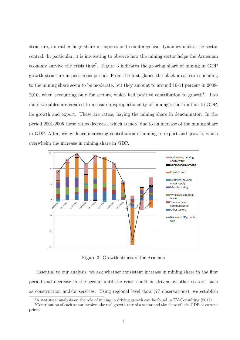
structure, its rather huge share in exports and countercyclical dynamics makes the sector

central. In particular, it is interesting to observe how the mining sector helps the Armenian

economy survive the crisis time7. Figure 3 indicates the growing share of mining in GDP

growth structure in post-crisis period. From the first glance the black areas corresponding

to the mining share seem to be moderate, but they amount to around 10-11 percent in 2008-

2010, when accounting only for sectors, which had positive contribution to growth8. Two

more variables are created to measure disproportionality of mining’s contribution to GDP,

its growth and export. These are ratios, having the mining share in denominator. In the

period 2001-2005 these ratios decrease, which is more due to an increase of the mining share

in GDP. After, we evidence increasing contribution of mining to export and growth, which

overwhelm the increase in mining share in GDP.

Figure 3: Growth structure for Armenia

Essential to our analysis, we ask whether consistent increase in mining share in the first

period and decrease in the second until the crisis could be driven by other sectors, such

as construction and/or services. Using regional level data (77 observations), we establish

7A statistical analysis on the role of mining in driving growth can be found in EV-Consulting (2011).8Contribution of each sector involves the real growth rate of a sector and the share of it in GDP at current

prices.

4

very poor correlation between mining and the main industry sectors9, except with trade

and service, −0.32 and −0.37, respectively. When checking for causal impacts from other

sectors’ share to mining, we get insignificant coefficients, except for agricultural share. These

are evidences, which support to the hypothesis that mining and its share in GDP can be

treated as an exogenous factor, which may have a significant power to explain GDP growth,

inequality and poverty dynamics for the Armenian economy10.

Analyzing mining’s contribution to the evolution of industry structure and related macroe-

conomics indicators provide useful insights. However, in order to estimate the impact of

mining, one needs to have a larger sample size and more details on variation of relevant

variables. For this reason we make use of regional level data on the annual base, which

covers the period 2004-2010. Armenia has 11 administrative districts, Yerevan (the capital)

and 10 marzes11. In effect we have 77 observations, which allows to estimate causal impact

of mining on growth, inequality and poverty.

We start with the description of our dataset and highlight some useful statistics on

productivities in Section 1. Section 2 discusses econometrics methods and issues we challenge.

Econometric analysis covers Section 3 and Section 5 concludes.

2 Data description

We use data from the National Statistical Service of the Republic of Armenia (NSSRA).

The second source of data is Household Survey micro database from 2004 to 2010, which

is representative for the whole population and includes from 4000 to 8000 households, de-

pending on a year12. From annual reports by NSSRA, we take marz level manufacturing,

construction, agriculture, trade and service shares, productivities and employment shares.

9We identify the following sectors for our analysis: mining, service, trade, agriculture, manufacturing andconstruction. Manufacturing involves mining.

10Nevertheless, our argument is far to be sufficient to exclude endogeneity of mining. We discuss the issuelater in the paper.

11In Armenian the term ”marz” stands for district (state) and we use it without translation.12Household survey data is available in NSSRA website, www.armstat.am.

5

Figure 4: The main export items for Armenia. Source: Kostanyan (2011)

As NSSRA is not publishing marz level GDP, we construct this data13. From Household

survay database we construct marz level data on different inequality measures, poverty rate,

remittances, and wage income. Some of the variables are not used in estimated models, but

we have tried to extract the highest explanatory power from the total set of variables, relevant

to our model specifications. We have 77 observations in total (7 years and 11 marzes).

We construct industry shares using marz GDP and industry value added at current

prices. A change in relative prices matter for consumption basket, and shares based on

nominal values capture movements in relative prices. Productivities are also calculated at

current prices. The GDP growth, nevertheless, is real, as the nominal factor may create

effects without counterfactors14.

In our analysis marzes have equal shares, while aggregate measures of the above variables

put population weights for marzes. As a matter of the fact, if we estimate a certain relation-

ship with corresponding findings using aggregate data, it may well differ from the findings of

13For details contact the author.14Wehn taking two nominal values, the impact of common price movements will be canceled out, and the

remaining effect will be due to relative price changes.

6

010

2030

mill

ions

AM

D

2004 2006 2008 2010year

Aragatsotn AraratArmavir GegharkunikKotayk LoriShirak SjunikTavush Vayots DzorYerevan

Figure 5: Mining productivities among marzes

panel based estimation of the same specification. This approach helps statistically evaluate

how effectively policies have been addressed towards balanced regional development, a central

concept for a long run growth strategy for the Armenian government15.

Figure 5 plots productivity in the mining sector in all marzez16. Syunik marz is distin-

guished by its high productivity. Some marzes, such as Shirak and Vayots Dzor, experienced

high productivity before the crises started, while there was a drop in productivity during the

crisis time. Some other marzes (Gegharkunik, Lori, Syunik) pattern the opposite dynamics,

low productivity before crisis and high after. Finally, there are marzes, which seem to be

indifferent to the crisis shock (Tavush, Kotayk etc).

Productivity of a certain mine is (i) product and (ii) mine specific. The third factor

is macroeconomic, the company may face at any time. As time unfolds, different events

15The Armenian government has endorsed set of measurements embedded in an official document ”Bal-anced regional development”, aimed at creating equal opportunities for all regions to develop infrastructuresand production capabilities.

16In fact, to be prices we should write in all 10 marzes and Yerevan. We treat the capital as a marz tosave space.

7

05.

000e

−08

1.00

0e−

071.

500e

−07

Den

sity

0 10000000 20000000 30000000

Productivity of manufacturingProductivity of mining

kernel = epanechnikov, bandwidth = 1.2e+06

Kernel density estimate

Figure 6: Productivities in mining and manufacturing

will alter initial productivities in certain ways, which will affect factor incomes, wages and

profits. In order to get some insights how productivity in mining sector evolves over time, we

plot distribution of marz specific productivities, manufacturing versus mining. Very rough

approximation will be to use productivity distribution as a proxy for earnings distribution

from the mining industry, as we do not have data for the latter.

For saving space, we only compare mining productivity with the manufacturing produc-

tivity. Also we plot dynamics of mining productivity distribution, before and during crisis

period. Figure 6 reflects the fact that in average productivity in mining falls short from that

of manufacturing. The second observation is that productivity variation in mining is higher

than that in manufacturing among marzes. It is worth recalling that in this and forthcoming

distributions all marzes have equal weights, while volumes of mining products may well differ

from one marz to the other. Though very preliminary, there can be drown four observational

implications from the above arguments:

1. If there is no a significant move in distribution towards a higher mean (median), then

an increase in mining share is expected to deprive growth.

2. If high inequality in productivity is translated to high factor income distribution in

8

05.

000e

−08

1.00

0e−

071.

500e

−07

Den

sity

0 5000000 10000000 15000000 20000000 25000000

Productivity of manufacturingProductivity of mining

kernel = epanechnikov, bandwidth = 1.4e+06

Kernel density estimate

Figure 7: Productivities in mining and manufacturing in 2004-2007

mining, then it is very likely that a higher share of mining in manufacturing will further

disequalize income among households.

3. If we draw a conventional poverty line for productivity, then simple expansion (not

based on productivity) of mining may lead to higher poverty, as more households will be

trapped in the poverty region.

4. Mining distribution is bimodal, implying that there are marzes with very high produc-

tivity, well separated from the average productivity.

These observations hinge on comparison between mining and manufacturing productiv-

ities. For an ideal comparison marz-economy specific productivity should be taken instead

of manufacturing. The problem is that productivities calculated above involves intermedi-

ate goods consumption and is not corrected for shadow economy. At the moment, we only

have data on marz level value added, which is net of intermediate goods consumption and

accounts for the shadow economy factor.

Next we plot productivity distributions for two subsamples, 2004-2007 and 2008-2010.

Figures 7 - 8 indicate the impact of crisis on mining’s productivity distribution. The second

mode has disappeared and the overall inequality has been mitigated - a higher mean and

9

05.

000e

−08

1.00

0e−

071.

500e

−07

Den

sity

0 10000000 20000000 30000000

Productivity of manufacturingProductivity of mining

kernel = epanechnikov, bandwidth = 1.4e+06

Kernel density estimate

Figure 8: Productivities in mining and manufacturing in 2008-10

lower variance is reported during the crisis period. It is then very likely, that mining helped

households to get out of the poverty region, if wages are paid according to productivities. We

also plot dynamics of mining’s productivity distribution to observe, how average productivity

evolves over time. Again, we take before crisis period and the crisis time. Figure 9 indicates

that we have much higher mean17 with almost no change in standard deviation. Thus, we

cannot exclude the scenario that expansion of mining may enhance growth, as the average

productivity has increased, while dispersion has decreased.

We close this section by the well known fact that formal regression analysis is needed to

establish causal effects, in our case, from mining sector to growth, inequality and poverty

measures. In fact, our observational implications serve as hypotheses for causal analysis.

Next we turn to the econometric model.

176,02 mln. versus 4,95 mln., in AMD.

10

05.

000e

−08

1.00

0e−

071.

500e

−07

Den

sity

0 10000000 20000000 30000000

Productivity of mining in 2004−2007Productivity of mining in 2008−2010

kernel = epanechnikov, bandwidth = 1.2e+06

Kernel density estimate

Figure 9: Dynamics of mining’s productivity

3 Econometric model

The general strategy is to search within the set of linear regression models, in which

mining has a significant role18. Our model takes the following form:

yi,t = α0 + βminingi,t + α1x1,i,t + ...+ αkxk,i,t + ui + ǫi,t; (1)

where the left hand side variable yi,t will stand for growth, inequality and poverty, depending

on a model. The variableminingi,t is the mining share in marz GDP, and x1,i,t, ..., xk,i,t are all

relevant variables for a given model. In particular, we will check for shares of other industries,

employment shares, variables from Household survey dataset, such as remittances, as well as

spatial factor of the dependent variable and time dummies. We take fixed effects approach

(ui captures fixed effects), in order to account for large unobserved differences among marzes.

The error term is ǫi,t. Finally, the subscripts i and t stand for a specific marz and a year,

respectively.

18Begrakyan and Grigoryan (2012) use the same dataset, looking at unrestricted models to explains incomeinequality and poverty.

11

The model in (1) has a great potential to suffer from the endogeneity problem. The way,

how the shares are constructed, introduce endogeneity. To see this, consider the following

scenario. Suppose service is not included in the model, as it has no significant explanatory

power on the left hand side variable. However, service expansion leads to contraction of

mining share almost by construction, as shares sum to 1. Then, if the impact of mining on

inequality (the dependent variable) can be sufficiently explained by the variation of service

share, mining becomes endogenous. The ultimate question will be which variable is relevant

to the model, as there is a functional link between mining and service shares. We control

for endogeneity to some extent - mining share is very small and it seems fairly independent

from most of the industry shares, as stated in Introduction.

Another issue is simultaneity in the model. Our strategy is to explain growth, inequality

and poverty by exogenous drifts in industry shares and other relevant variables. We do

not claim that there are no tendencies in the industry structure, but our primary concern

is to explain the dynamics of inequality and poverty by mostly exogenously driven part

of structural change. If there is, however, a long term component in variables, it will be

captured too, since in fact we explore a long term cointegration relationship in most of the

specifications. We do not detrend our variables, but instead allow to capture comovements,

which in part owes to persistence in the data generating process. The main reason why we

do not decompose our data into trade and stochastic components, is a very limited time

span.

We learn the extent of persistence in main variables, using Bias-corrected the least squares

dummy variable (LSDV) method19, to estimate AR(1) processes. Inequality measures are

relatively less persistent than poverty, and for the latter time dummies are very informative.

Growth is not persistent - its lagged value is insignificant. Parallel to the benchmark model

19The Stata routine has been written by Bruno (2005). The general idea goes back to Kiviet (1995), whosuggest to use a consistent estimator for the true parameter, in order to control for the bias, generated whenestimating dynamic models by least squares.

12

in (1), we also check for the following relationship:

yi,t = ρyi,t−1 + (1− ρ)(α0 + βminingi,t + α1s11,i,t + ...+ αks

kk,i,t) + ui,t + ǫi,t, (2)

where s11,i,t, ..., skk,i,t are the residuals of corresponding AR(1) estimates for xj,i,t variables. A

part of endegeneity is removed, as the current shocks are embedded in the model. However,

current shocks may well be endogenous to current variables, excluded from the model. This

specification is not much different from dynamic panel models studied by Arellano and Bond

(1991) and Blundell and Bond (1998), among others20.

Unfortunately, specifications in form of (2) do not yield significant estimates, and instead

we use the modification of that model for the growth equation only:

sgrowthi,t = α0 + βminingi,t + α1s

11,i,t + ...+ αks

kk,i,t + ui,t + ǫi,t, (3)

where sgrowthi,t is the residual from the AR(1) estimate of growth.

The last issue, we want to control for our models is the small sample size. We control

finite simple properties for our models by bootstrap analysis, with the number of replications

10000. If an estimated model passes the normality test, then standard errors corrected by

bootstrap will not significantly differ from the estimated once and the model will pass the

test21. That is, we use bootstrap analysis to check models’ sensitivity to finiteness of the

sample22. For each estimated model, we report bootstrap corrected standard errors to check

validity of the model. Standard errors, corrected by bootstrap are very sensitive to number

of observations and for this reason we do not test our models for subsamples, as too few

observations will be left for a test.

20We do not estimate classical dynamic panel models by GMM, as the number of cross sections is extremelysmall, and the estimated coefficients would suffer in huge bias.

21For bootstrap procedures, see Cameron and Trivedi (2010), Chapter 13.22We can call it a test for stability of a model.

13

4 Estimation

Growth model

Reported estimates for different growth specifications are in Table 1. As hypothesized

above, an accelerated expansion of mining is indeed growth enhancing. The significance for

the coefficient is rather on the margin, but it well survives the bootstrap test. The benchmark

specification (Column 1) also involves agricultural, construction and service shares, as well

as export and import shares. All variables are in percentages, within the range 0− 100, and

the estimated coefficients reflect the percentage point (pp) change for growth, as a response

to 1 percentage point change in an independent variable. In particular, 1 pp increase in

mining shares, say from 3% to 4%, will lead to 4.418 pp in growth.

Is this a big number? In our context, one needs to disentangle two factors which may

drive growth. There can be no structural change in an economy under positive growth, as

each sector grows by the same rate (balanced growth). The second factor is the change in the

industry structure, and if there is a structural break in an economy, which leads to a higher

growth, the corresponding causality will be established. It is possible to draw scenarios, in

which 1 pp change in certain industry share, no matter how small the industry is, leads to

any reasonable pp change in growth23. In general, the coefficient of the mining share, 4.418,

is a pretty big number and comes to confirm statistical evidence from Table 2.

23In order to control for the impact of the sectoral growth, we need to use these components as explanatoryvariables.

14

Table 1: Growth specifications

(1) (2) (3) (4) (5) (6)benchmark boot.(1) Syunik excl-ed boot.(3) weighted shock appr.

mining 4.418∗ 4.418∗ 2.405∗∗∗ 2.405 4.089∗∗ 5.9624∗∗∗

(2.338) (2.368) (.500) (2.105) (2.042) (1.251)

agr .996∗∗∗ .996∗∗ .976∗∗∗ .976∗∗ 1.145∗∗∗ .826∗∗

(.200) (.434) (.175) (.442) (.150) (.344)

const 1.598∗∗∗ 1.598∗∗∗ 1.692∗∗∗ 1.692∗∗∗ 1.810∗∗∗ 1.808∗∗∗

(.428) (.551) (.372) (.533) (.149) (.394)

serv 2.122∗∗ 2.122 1.932∗ 1.932 1.277(.962) (1.292) (1.091) (1.341) (.813)

export 1.511∗∗∗ 1.511∗∗ 1.911∗∗∗ 1.911∗∗ 1.600∗∗∗ .661(.309) (.643) (.371) (.751) (.169) (.405)

import -2.388∗∗∗ -2.388∗∗ -2.532∗∗∗ -2.532∗∗∗ -2.498∗∗∗ .976∗∗∗

(.675) (.990) (.647) (.971) (.357) (1.251)

N 77 77 70 70 77R2: within .261 .261 .323 .323 .547∗− 90%, ∗∗

− 95% ∗∗∗− 99%

Interestingly, all other covariates have much less impact on growth. This is indeed an

evidence, how important mining is for growth. There is much capacity in mining to boost

growth. Column 2 confirms that the benchmark specification is robust to small sample

size. We estimate the same model in Column 3 without Syunik marz. The difference is

striking - almost 50% of mining’s contribution to growth acrues to Syunik marz. Although

this estimate does not pass the bootstrap test24, but the result seems to be reasonable.

A huge share of mining industry is concentrated in Syunik, and this comes natural that

mines in Syunik comprise the driving power of the mining industry for growth. We use

population weights for becnhmark specification in Column 5. As we can see, the magnitudes

of coefficients are almost identical. In the last column we estimate the model (3) and,

interestingly, the impact of the mining share is even stronger, when persistence of both

variables is controled. That is, if we explain the part of growth, which is net of inertia,

then an increase in mining share, purely driven by current factors, will result in even higher

24A decrease in coefficient has not been accompanied by a corresponding decrease in the standard error,which is an evidence of the relevance of the Syunik marz, as its portion in the standard deviation turns tobe smaller relative to the rest of the eocnomy. This can be seen, when mooving from Column 4 to 2 in Table1.

15

growth.

Overall, the growth model captures common perception that mining is important for

growth. As noted earlier, there is much endogeneity in the model, which mainly comes

from other industry shares, but we expect that the bias of the mining coefficient is small

enough to capture reality. It does, as the magnitude of the estimated coefficient reflects the

huge disproportionality between the mining share in GDP and its contribution to growth,

indicated in Table 2.

Inequality model

We have seen that mining is growth enhancing. Then the question is whether mining

driven growth is pro-poor. Unfortunately, there is no evidence that mining expansion will

help equalize income among households. The impact of mining on resource distribution

is twofold. The direct effect is reflected by factor income distribution in mining, in forms

of wage and profit distributions. The indirect effect is related to externalities created and

amplified along the expansion of existing mines and exploitation of the new once. The

damage by mining is usually underestimated and the mine owners do not totally internalize

the negative consequences, resulting in deterioration of natural and local resources. This

may increase inequality, as well as poverty.

Specifications for inequality models are in Table 2. All models involve mining agricultural

and service shares, and a dummy variable for the year 2007. The inequality measure is the

Gini index.

Mining’s expansion seems to increase inequality. If there will be 10% percent in increase

in value added in mining, which will lead to around 0.25 pp increase in mining share, then

Gini index will increase by 0.17 pp. Again, if we want to qualify the impact, we may compare

the coefficient of mining share with those of agricultural and service shares, controlling for

share differences. The share of agriculture is around 11 times higher than the share of

mining. Instead, the coefficient of mining share is even higher than that of agricultural

16

share. In effect, the coefficient of mining is 14 times larger than that of agricultural share

and 3.7 times larger than the coefficient of the service share.

Table 2: Inequality specifications

(1) (2) (3) (4) (5) (6)benchmark boot(1) altern. boot.(3) Syunik excl. boot.(5)

mining .666∗∗∗ .666 .670∗∗∗ .670 .679∗∗∗ .614(.102) (.532) (.157) (.433) (.129) (.719)

agr .542∗∗∗ .542∗∗∗ .688∗∗∗ .688∗∗∗ .545∗∗∗ .690∗∗∗

(.145) (.152) (.202) (.191) (.154) (.203)

const .466∗∗∗ .466∗∗∗ .551∗∗∗ .551∗∗∗ .476∗∗∗ .557∗∗∗

(.136) (.163) (.173) (.191) (.137) (.197)

d2006 -4.181∗∗∗ -4.181∗∗∗ -4.359∗∗ -4.359∗∗∗ -4.793∗∗∗ -4.948∗∗∗

(1.556) (1.385) (1.875) (1.537) (1.559) (1.608)

N 77 77 77 77 70 70R2: within .302 .302 .386 .386 .323 .399∗− 90%, ∗∗

− 95% ∗∗∗− 99%

The bootstrap test, however, indicates that estimated coefficients are sensitive to the

sample size. The significance level is around 20% with the P-value ≈ 0.80 , which is still an

evidence that mining has a causal impact on income inequality. When using an alternative

measure for Gini index25, we obtain similar coefficients. After, we exclude Syunik marz from

our sample, but the exclusion does not lead to any significant change in the model. This

is an evidence, that mining industry does not generate excessive inequality relative to the

rest of the industry. Again, bootstrap test indicates that the estimated coefficients lacks in

acceptable significance.

Poverty model

Begrakyan and Grigoryan (2012), using the same dataset, argue that poverty dynamics is

basically explained by the spatial factor, which is further expelled, when time dummies are

introduced26. They do not check for mining share as a separate covariate, while concentrating

25The difference is about weights, used to move from houseolds’ income to per capita income.26The authors start with a multiplicative model and use the log form. We do not use the log form of the

model, as almost in non of the specifications mining is significant. The reason is that log values of very smallnumbers do not ensure sufficient variation and hence lack in explanatory power.

17

only on the main 4 sectors, agriculture, manufacturing, service and construction. It is

interesting to find out that mining has a significant impact on poverty, even if we control for

the spatial factor and time dummies. In the benchmark specification, 1 pp increase in mining

share leads to 0.67 pp increase in the poverty rate27. The magnitude is very close to that in

the inequality model. The causal impact of mining to inequality is almost as strong as that

of the spatial factor28. The latter passes the bootstrap test, while mining share sustains 15

percent significance level. As in Begrakyan and Grigoryan (2012), when time dummies are

introduced, the spatial factor becomes redundant. Surprisingly, the coefficient of the mining

share continues to be significant, which is an evidence of the strong impact of mining on

poverty.

Table 3: Poverty specifications

(1) (2) (3) (4) (5) (6)benchmark boot(1) Synik excl-ed boot.(3) year dummies boot.(5)

mining .672∗∗ .672 .554 .554 .557∗∗ .557(.318) (.416) (.384) (.874) (.247) (.359)

povsp .845∗∗∗ .845∗∗∗ .853∗∗∗ .853∗∗∗

(.110) (.095) (.123) (.100)

d2005 -4.781∗∗∗ -4.781∗∗∗

(.864) (1.076)

d2006 -6.985∗∗∗ -6.985∗∗∗

(1.139) (1.167)

d2007 -10.474∗∗∗ -10.474∗∗∗

(1.347) (1.230)

d2008 -10.512∗∗∗ -10.512∗∗∗

(1.318) (1.311)

N 77 77 70 70 77 77R2: within .622 .622 .618 .618 .705 .705∗− 90%, ∗∗

− 95% ∗∗∗− 99%

When Syunik marz is excluded from the sample, the impact becomes insignificant. Thus,

mining in Syunik makes the industry generate poverty. An immediate conclusion is that

wages in mines located in Syunik fall short to keep households out of the poverty region.

This should be a serious concern for policy makers, as boosting mining, in particular in

27Poverty rate is the poverty headcount ratio at US $2 a day, as a percentage of population, PPP adjusted.28The spatial variable is constructed as an average of inequality rates from neighboring marzes.

18

Syunik, will accelerate growth, but it entail higher poverty.

5 Conclusion

In this paper we search for econometric models for growth, inequality and poverty, in

which mining sector has a significant role. We dare to take such an approach, as there

is common perception that mining in Armenia has a specific role for the economy. First,

it has served as a buffer for mitigating the disastrous impact of the world financial crisis.

Second, mining comprises more than 20 percent of the Armenian exports and it has a growing

tendency. Third, mining seems to be far from its capacity utilization and its share in GDP

is growing too.

To our knowledge, there is no paper which quantifies the causal impact of mining (share)

on growth, inequality and poverty for Armenia. Our paper is of descriptive nature, but it has

certain normative implications. Variation of mining, both in terms of growth and industry

share, entails social consequences. Mining sector is an externality creator, a big concern

from the social viewpoint29. In this context the trade-off between growth (efficiency) and

inequality/poverty (equity), takes an extreme form, as the two components seem to pattern

zero complementarity. Our econometric analysis highlight this trade-off effectively - mining

is growth enhancing, but it does bad job for inequality and poverty. That it is growth

enhancing, may tempt the current government encourage further expansion of mining. This,

however, conflicts with the equity consideration, and the government should draw certain

policies to impose mining companies taking responsibilities of social consequences.

For controlling negative impact of mining expansion on inequality and poverty in the long

run, total compensation of environmental damage by mines should be a strong precondition

for exploitation. For poverty reduction in the short run, wages are of primary concern. Also,

local community should definitely benefit from mining through different social programs, as

a (non-exhaustive) part of mining companies’ social responsibility.

29For the theory of externalities, see Mas-Colell et al. (1995).

19

Our results can be improved in different directions. A very limited time span makes the

estimates highly sensitive to structural changes. We check for sensitivity by bootstrapping

standard errors, but this is a poor prescription to finite sample problem. We have regional

level data, but number of regions is very limited and we cannot use dynamic panel approach,

by this effectively controlling for endogeneity. We make certain judgments on the extent of

endogeneity we may have in models, but do not formally control for it.

Will all these deficiencies in mind, the model implied results are in line with common

perceptions and concerns, present in Armenia. We believe this is the central finding of the

paper, among others.

References

Manuel Arellano and Stephen Bond. Some tests of specification for panel data: Monte carlo

evidence and an application to employment equations. Review of Economic Studies, 58

(2):277–97, April 1991.

Edgar Begrakyan and Aleksandr Grigoryan. Inequality, growth and industry structure:

Evidence from armenia. Technical report, AUA, CBA, December 2012.

R Blundell and Steven Bond. Initial conditions and moment restrictions in dynamic panel

data model. Technical report, 1998.

Giovanni S.F. Bruno. Estimation and inference in dynamic unbalanced panel data mod-

els with a small number of individuals. KITeS Working Papers 165, KITeS, Centre for

Knowledge, Internationalization and Technology Studies, Universita’ Bocconi, Milano,

Italy, June 2005.

A. Colin Cameron and Pravin K. Trivedi. Microeconometrics Using Stata, Revised Edition.

Number musr in Stata Press books. StataCorp LP, July 2010.

20

EV-Consulting. Counturs of armenia’s economy in 2010: mining drives growth. EV Period-

ical, (2), April 2011.

IMF. Republic of armenia: Poverty reduction strategy paper. IMF Country Report, 11(191),

2011. URL http://www.imf.org/external/pubs/ft/scr/2011/cr11191.pdfl.

Jan F. Kiviet. On bias, inconsistency, and efficiency of various estimators in dynamic panel

data models. Journal of Econometrics, 68(1):53–78, July 1995.

Tigran Kostanyan. Export expansion and diversification in armenia. Technical report, World

Bank, December 2011. URL http://acf.eabr.org/media/img/eng/Development_

Partners/Kostanyan_eng.pdf.

A. Mas-Colell, M. Winston, and R. Green. Microeconomic Theory. 1995.

Nienke Oomes, Gohar Minasyan, and Ara Stepanyan. In search of a dramatic equilibrium:

Was the armenian dram overvalued? IMF Working Papers 09/49, International Monetary

Fund, March 2009. URL http://ideas.repec.org/p/imf/imfwpa/09-49.html.

21