Recent Landsat Calibration Updates

Dennis HelderLandsat Science Team Meeting

Boise, IdahoJune 16, 2010

Topics• Landsat 5 TM Relative Gain Update

– An example of the value of the Landsat Image Assessment System

• Landsat 4 TM MTF Corrrection– Restoring data never seen by mortals

• MSS Absolute Calibration– The final(?) word

Acknowledgements– Landsat Project Science Office, GSFC– USGS EROS– SDSU Image Processing Lab

L5TM Relative Gains

J.Dewald

The IAS and Relative Gains• The Landsat Image Assessment System provides a quality check on

every image processed at USGS EROS– Pertinent calibration information is extracted from each scene, cal file,

and metadata– This information provides long and short term trending information that

is invaluable for calibration updates– Literally 10’s of 1000’s of data points can be obtained for any cal

parameter• Detector Relative Gains are a primary source of striping in Landsat

Imagery– Various methods of calculating these values have been used including

on-board cal lamps, scene-based equalization, and lifetime trending– The IAS collects data on the relative response of each detector for each

scene– Very dense data sets, properly filtered, have allowed accurate model

development over the lifetime of Landsat TM instruments.

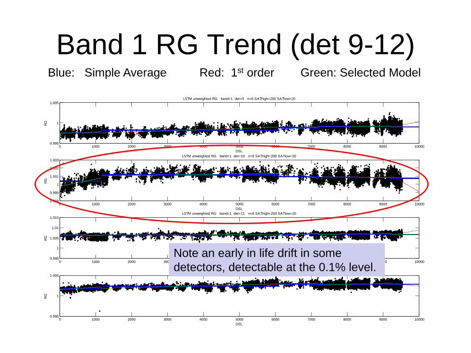
Band 1 RG Trend (det 9-12)

0 1000 2000 3000 4000 5000 6000 7000 8000 9000 100000.995

1

1.005

DSL

RG

L5TM unweighted RG band=1 det=9 n=6 SAThigh=200 SATlow=20

0 1000 2000 3000 4000 5000 6000 7000 8000 9000 100000.998

0.999

1

1.001

1.002

1.003

DSL

RG

L5TM unweighted RG band=1 det=10 n=6 SAThigh=200 SATlow=20

0 1000 2000 3000 4000 5000 6000 7000 8000 9000 100000.995

1

1.005

1.01

1.015

DSL

RG

L5TM unweighted RG band=1 det=11 n=6 SAThigh=200 SATlow=20

0 1000 2000 3000 4000 5000 6000 7000 8000 9000 100000.995

1

1.005

DSL

RG

L5TM unweighted RG band=1 det=12 n=6 SAThigh=200 SATlow=20

Blue: Simple Average Red: 1st order Green: Selected Model

Note an early in life drift in some detectors, detectable at the 0.1% level.

Band 4 RG Trend (det 13-16)

0 1000 2000 3000 4000 5000 6000 7000 8000 9000 100000.98

0.985

0.99

0.995

1

1.005

DSL

RG

L5TM unweighted RG band=4 det=13 n=6 SAThigh=200 SATlow=5

0 1000 2000 3000 4000 5000 6000 7000 8000 9000 100000.985

0.99

0.995

1

1.005

DSL

RG

L5TM unweighted RG band=4 det=14 n=6 SAThigh=200 SATlow=5

0 1000 2000 3000 4000 5000 6000 7000 8000 9000 100000.99

0.995

1

1.005

1.01

1.015

DSL

RG

L5TM unweighted RG band=4 det=15 n=6 SAThigh=200 SATlow=5

0 1000 2000 3000 4000 5000 6000 7000 8000 9000 100000.98

0.985

0.99

0.995

1

1.005

DSL

RG

L5TM unweighted RG band=4 det=16 n=6 SAThigh=200 SATlow=5

Note in this case step discontinuities up to 1%. These will definitely cause striping!

Band 5 RG Trend (det 9-12)

0 1000 2000 3000 4000 5000 6000 7000 8000 9000 100000.995

1

1.005

1.01

1.015

DSL

RG

L5TM unweighted RG band=5 det=9 n=4 SAThigh=200 SATlow=5

0 1000 2000 3000 4000 5000 6000 7000 8000 9000 100000.96

0.98

1

1.02

DSL

RG

L5TM unweighted RG band=5 det=10 n=4 SAThigh=200 SATlow=5

0 1000 2000 3000 4000 5000 6000 7000 8000 9000 100000.98

0.99

1

1.01

DSL

RG

L5TM unweighted RG band=5 det=11 n=4 SAThigh=200 SATlow=5

0 1000 2000 3000 4000 5000 6000 7000 8000 9000 100000.99

0.995

1

1.005

1.01

1.015

DSL

RG

L5TM unweighted RG band=5 det=12 n=4 SAThigh=200 SATlow=5

In Band 5 observe a long term drift of 2%--large enough to cause objectionable striping…

2001 Day-207 Band-5

w/o RG correction

current RG correction

new RG correction

An example of removing the long term drift in relative gain occurring in Band 5.

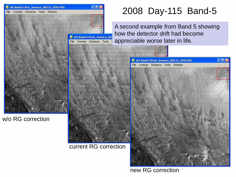
2008 Day-115 Band-5

w/o RG correction

current RG correction

new RG correction

A second example from Band 5 showing how the detector drift had become appreciable worse later in life.

2/25/2010 Band 5 L1GOld RG: S12605New RG: S12606

Current Models New Models

A Level 1G band 5 example from 2010. Note ‘diagonal striping pattern is removed.

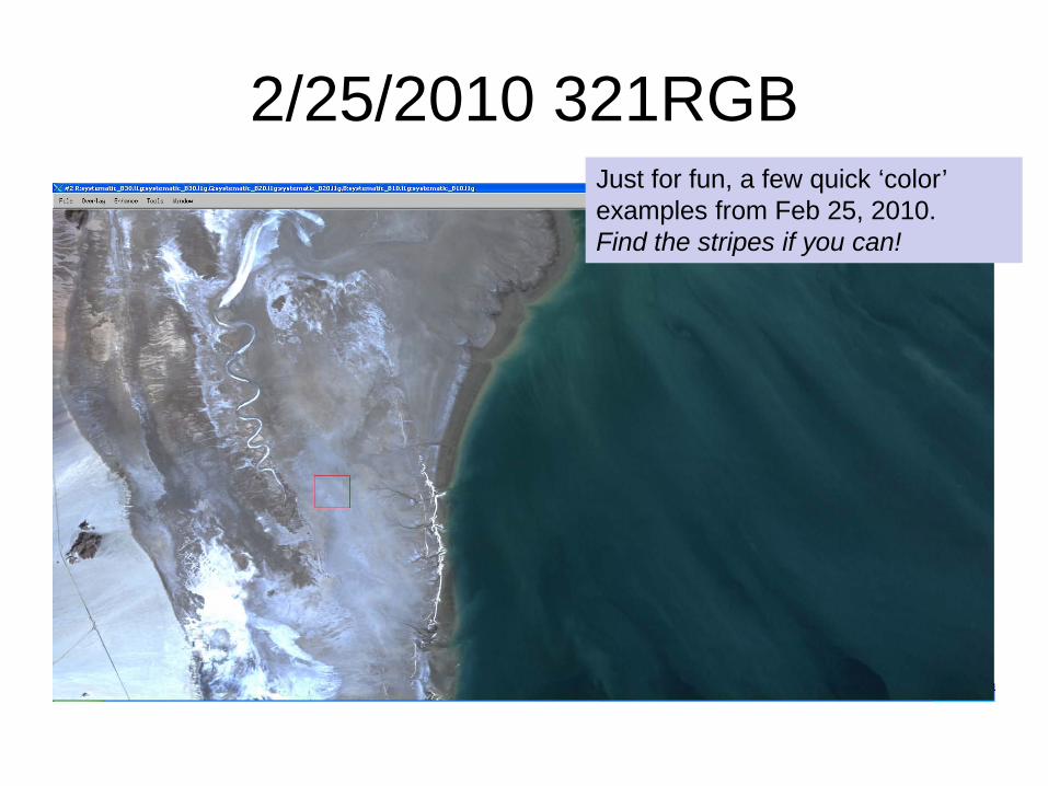
2/25/2010 321RGBJust for fun, a few quick ‘color’ examples from Feb 25, 2010.Find the stripes if you can!

2/25/2010 754RGB

2/25/2010 754RGB

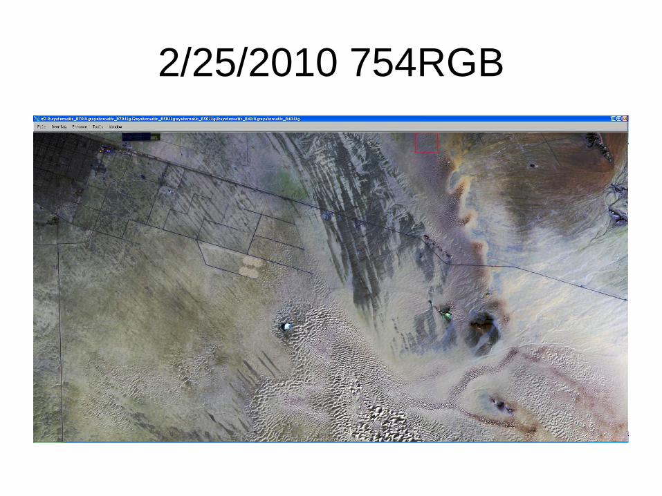
2/25/2010 754RGB

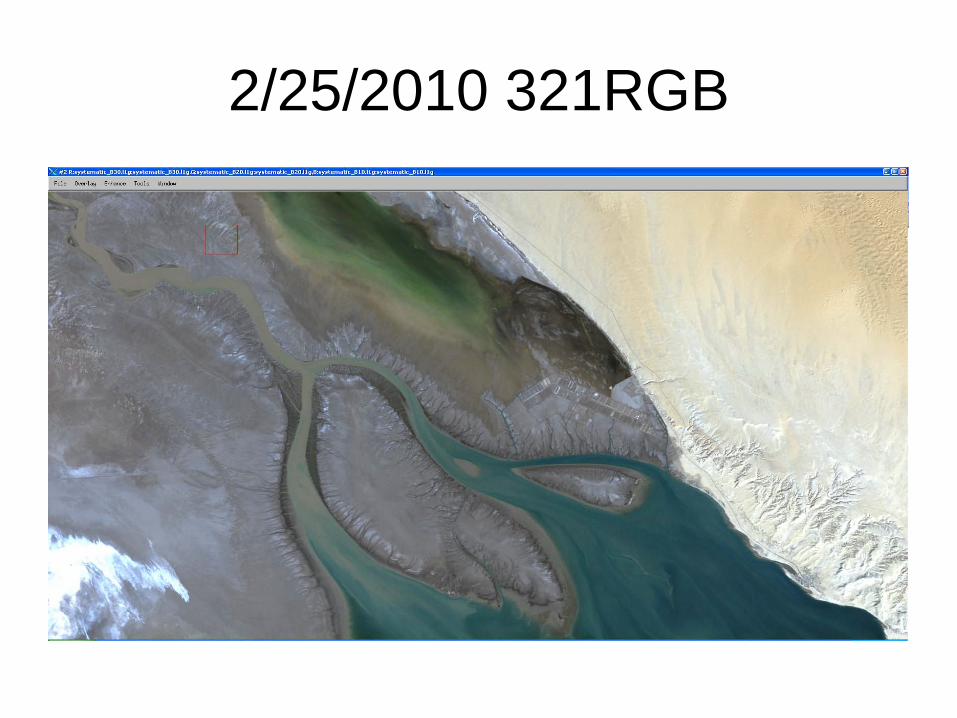
2/25/2010 321RGB

Landsat 4 Relative MTF Characterization/Correction

Dennis HelderDinesh Shilpakar

Cody AndersonImage Processing Laboratory

EECS DepartmentSouth Dakota State University

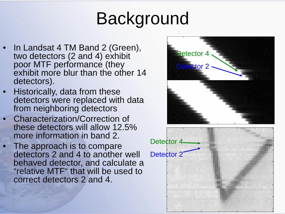
Background• In Landsat 4 TM Band 2 (Green),

two detectors (2 and 4) exhibit poor MTF performance (they exhibit more blur than the other 14 detectors).

• Historically, data from these detectors were replaced with data from neighboring detectors

• Characterization/Correction of these detectors will allow 12.5% more information in band 2.

• The approach is to compare detectors 2 and 4 to another well behaved detector, and calculate a “relative MTF“ that will be used to correct detectors 2 and 4.

Detector 4

Detector 2

Detector 4

Detector 2

20

Calibration Pulse Response used for Relative MTF Characterization

Detectors 2 and 4 are the “bad” detectors. Detector 6 is the reference detector that will be used to adjust detectors 2 and 4.

-50 0 50 1000

0.1

0.2

0.3

0.4

0.5

0.6

0.7

0.8

0.9

1

Normalized "Average" Cal Pulse Plot for Detectors 2 4 6

Pixel

Nor

mal

ized

Mag

nitu

de

246

Detector 4

Detector 2

0 0.05 0.1 0.15-1

-0.9

-0.8

-0.7

-0.6

-0.5

-0.4

-0.3

-0.2

-0.1

0

Det-2Det-4

0 0.05 0.1 0.150

0.2

0.4

0.6

0.8

1

Det-2Det-4

Final Relative MTF Estimate of Detectors 2 and 4

Normalized Freq

Nor

mal

ized

Mag

nitu

deP

hase

• Magnitude

• Phase

Normalized Freq

0 0.05 0.1 0.15 0.2 0.25 0.3 0.35 0.4 0.45 0.50

0.2

0.4

0.6

0.8

1

Det-2Det-4

0 0.05 0.1 0.15 0.2 0.25 0.3 0.35 0.4 0.45 0.50

0.2

0.4

0.6

0.8

1

g p

Det-2Det-4

Butterworth Tailed Relative MTF

Cut-off @ 0.104/pixel

Mag

nitu

de

• Butterworth Filter:

• Helps reduce the ringing effect in the corrected image.

• Correction is best for order 2. Higher orders provide significantly less correction.

nuDD

uB 20 )/(11)(

+=

D0 = cut-off freqDu = freq from centern = order of filter

R-MTF response with straight cut-off

R-MTF response with tailed Butterworth order -2

Butterworth Order 2

• For each scan line, the FFT of detectors 2 and 4 must be found.

• The FFTs of detectors 2 and 4 are divided by their estimated relative MTF.

• The IFFT is then taken and the corrected data is inserted back into the image.

• There are 374 scan lines in a scene, so 748, 6357 point FFTs and inverse FFTs are calculated for every scene.

• 6357 is the fixed length of MTF response model. This was derived from the maximum length of a valid scan line plus an extra buffer.

• Entire process takes ~1.5 seconds on a 3 GHz desktop machine!!

Correction Process

• Some Visual Treats

Results

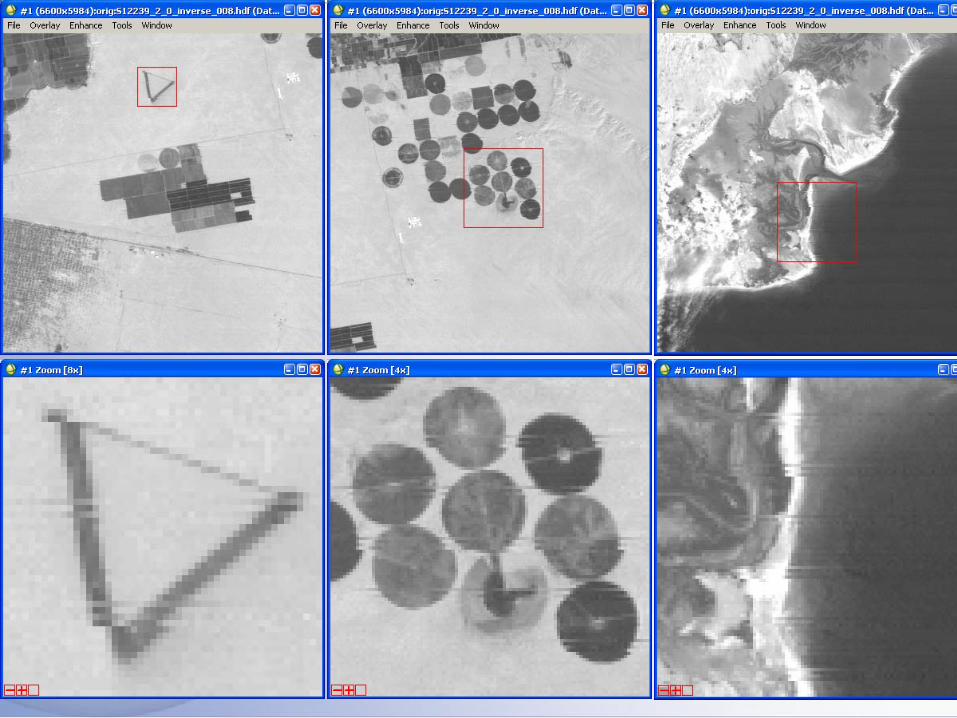
Sonoran Desert, Baja California

• Acquired on 11/25/1990

• Homogenous desert site often used for satellite calibration.

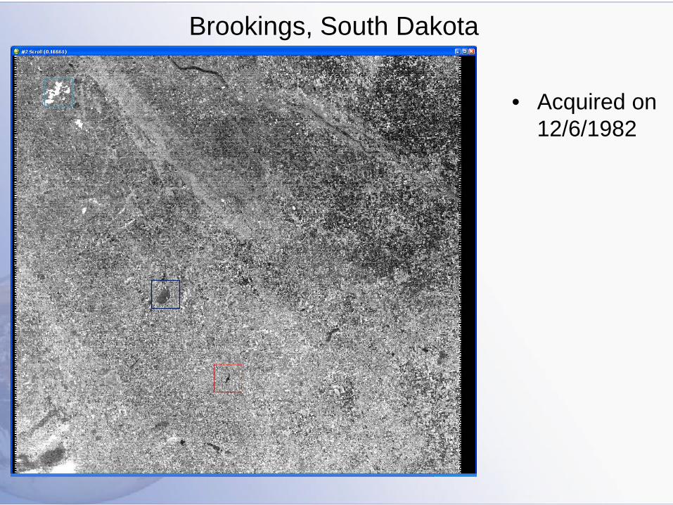
Brookings, South Dakota

• Acquired on 12/6/1982

Before

After

Libya-4, Africa

• Acquired on 3/18/1988

• Homogeneous Regions.

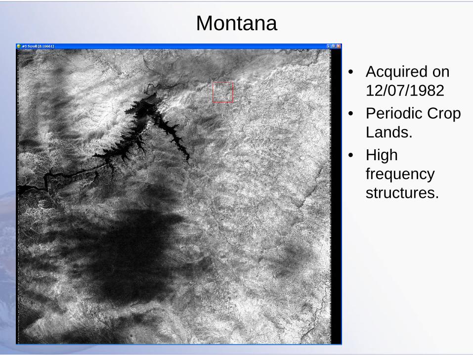
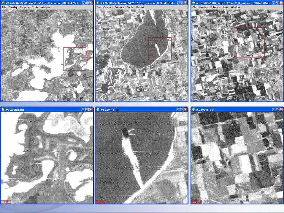
Montana

• Acquired on 12/07/1982

• Periodic Crop Lands.

• High frequency structures.

• Before

• After

“The Whole Ball of Wax”A Complete Landsat Calibration

• Dave Aaron• Ben Jasinski• Sadhana Karki

Recall from previous meetings…

• Landsat 5 TM cross-calibrated to Landsat 7 ETM+• Landsat 4 TM cross-calibrated to Landsat 5 TM• Landsat 1-5 MSS instruments cross-calibrated

sequentially to Landsat 5 MSS• Missing Piece: Absolute Calibration of MSS

series. Approach…– Use simultaneous collects of Landsat 5 TM and MSS

data over stable calibration site—Sonora Desert– Use Hyperion to account for spectral differences

SonoraDesert

ROI

MSS1:TM2 MSS2:TM3 MSS3:TM4 MSS4:TM4

Reflectance Radiance Reflectance Radiance Reflectance Radiance Reflectance Radiance

ROI #1 1.06 1.05 1.02 1.00 1.08 0.90 1.04 1.31

ROI #2 1.06 1.05 1.02 1.00 1.08 0.90 1.04 1.30

ROI #3 1.06 1.04 1.02 1.00 1.08 0.90 1.05 1.32

Sonora Desert SBAF Results

Atmospheric Effect SBAF BRDF

ROI Jitter

Total Uncertainty estimates

Band-1 4.3% 1.1% 0.3% 0.3% ~4.5%

Band-2 3.4% 0.8% 0.4% 0.6% ~4.0%

Band-3 4.4% 1.4% 0.7% 0.8% ~5.0%

Band-4 11.4% 3.0% 0.7% 0.3% ~12.0%

Uncertainty Estimates for Landsat Cross Calibration

Taking into consideration:Atmospheric Differences between ScenesSpectral Differences between ScenesTarget GeometryROI Misregistration Sensitivity

MSS Band 1 Results

100

110

120

130

140

150

160

170

1972 1977 1982 1987 1992

TOA

Nor

mal

ized

Rad

ianc

e (W

/m2u

msr

)

Year

Landsat 1-5 MSS Band-1 TM Band-2 (Spectral Radiance Vs Time)

Landsat-1 Landsat-2 Landsat-3Landsat-4 Landsat-5 Landsat-5 TM Band 2Landsat-4 TM Band 2

L-1μ=154.84

L-2μ=139.78

L-3μ=141.72

L-4μ=133.69

L-5μ=151.74

L-5 TM Band 2μ=131.81

L-4 TM Band 2μ=136.34

Before cross-calibration

applied

After cross-calibration

applied

100

110

120

130

140

150

160

170

1972 1977 1982 1987 1992

TOA

Nor

mal

ized

Rad

ianc

e (W

/m2u

msr

)

Year

TOA Radiance Derived over Sonoran Desert as seen by Landsat 1- 5 since 1972, Band-1

(Cross Calibrated to Landsat TM 5 )

Landsat-1 Landsat-2 Landsat-3Landsat-4 Landsat-5 Landsat-5 TM Band 2Landsat-4 TM Band 2

L-1μ=133.27

L-2μ=133.17

L-3μ=132.69

L-4μ=126.31

L-5μ=132.63

L-5 TM Band 2μ=131.81

L-4 TM Band 2μ=136.34

1 sigma uncertainty ~2%

MSS Band 2 Results

Before cross-calibration

applied

After cross-calibration

applied

Band 2

100

110

120

130

140

150

160

170

180

190

200

1972 1977 1982 1987 1992

TOA

Nor

mal

ized

Rad

ianc

e (W

/m2u

msr

)

Year

Landsat 1-5 MSS Band-2 TM Band-3(Spectral Radiance Vs Time)

Landsat-1 Landsat-2 Landsat-3Landsat-4 Landsat-5 Landsat-5 TM Band 3Landsat-4 TM Band 3

L-1μ=173.17

L-2μ=158.20

L-3μ=162.35

L-4μ=149.09 L-5

μ=161.41

L-5 TM Band 3μ=152.81

L-4 TM Band 3μ=146.2

100

110

120

130

140

150

160

170

180

190

200

1972 1977 1982 1987 1992

TOA

Nor

mal

ized

Rad

ianc

e (W

/m2u

msr

)

Year

y 1- 5 since 1972, Band-2

(Cross Calibrated to Landsat TM 5 )

Landsat-1 Landsat-2 Landsat-3Landsat-4 Landsat-5 Landsat-4 TM Band 3Landsat-5 TM Band 3

L-2u=150.12

L-3μ=149.47

L-4μ=147.77

L-5μ=148.48L-1

μ=151.31

L-5 TM Band 3μ=152.81

L-4 TM Band 3μ=146.2

1 sigma uncertainty ~2-3%

MSS Band 3 Results

80

90

100

110

120

130

140

150

160

170

180

1972 1977 1982 1987 1992

TOA

Nor

mal

ized

Rad

ianc

e(W

m-2

um-1

sr-1

)

Year

Landsat 1-5 MSS Band-3 and TM Band-4 (Spectral Radiance vsTime)

Landsat-1 Landsat-2 Landsat-3Landsat-4 Landsat-5 Landsat-5 TM Band 4Landsat-4 TM Band 4

L-1μ=144.49

L-2μ=141.61

L-3μ=135.34

L-4μ=133.59

L-5μ=142.64

L-5 TM Band 4μ=120.48

L-4 TM Band 4μ=119.88

Before cross-calibration

applied

After cross-calibration

applied

Band 3

80

90

100

110

120

130

140

150

160

170

180

1972 1977 1982 1987 1992

TOA

Nor

mal

ized

Rad

ianc

e (W

/m2u

msr

)

Year

y 1- 5 since 1972, Band-4

(Cross Calibrated to Landsat TM 5 )

Landsat-1 Landsat-2 Landsat-3Landsat-4 Landsat-5 Landsat-4 TM Band 4Landsat-5 TM Band 4

L-1μ=118.61

L-2μ=120.35

L-3μ=140.12

L-4μ=120.30

L-5μ=122.6

4

L-5 TM Band 4μ=120.48

L-4 TM Band 4μ=119.88

1 sigma uncertainty ~3%

MSS Band 4 Results

10

30

50

70

90

110

130

150

1972 1977 1982 1987 1992

TOA

Nor

mal

ized

Rad

ianc

e (W

/m2u

msr

)

Year

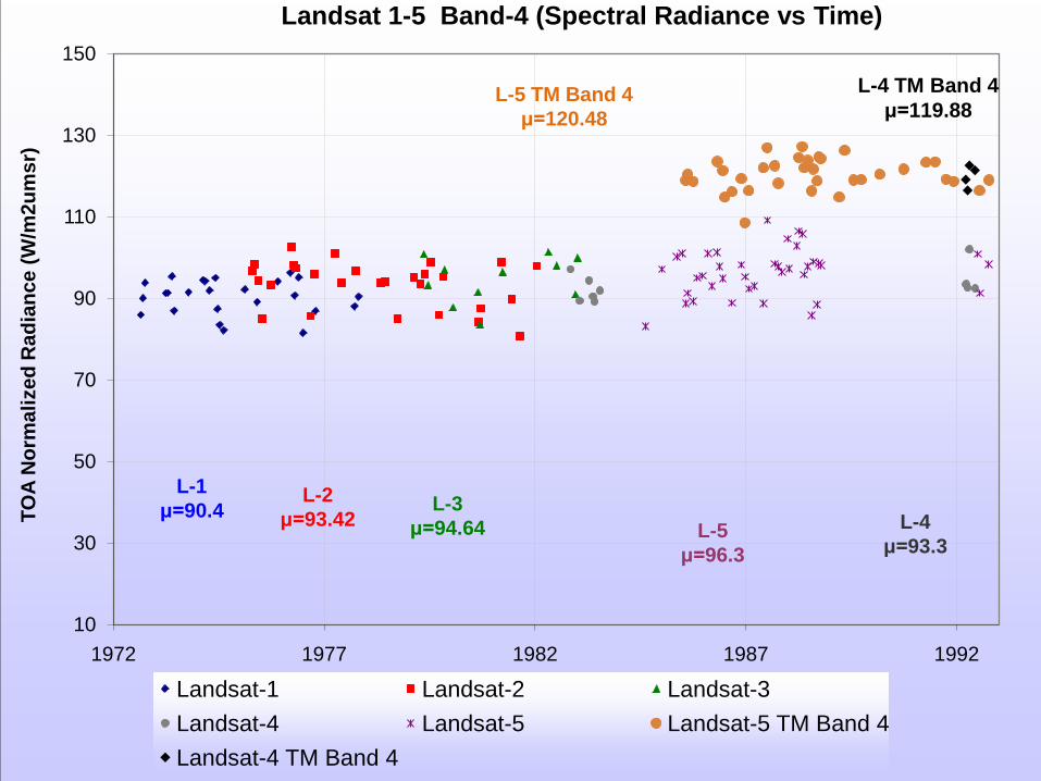
Landsat 1-5 Band-4 (Spectral Radiance vs Time)

Landsat-1 Landsat-2 Landsat-3Landsat-4 Landsat-5 Landsat-5 TM Band 4Landsat-4 TM Band 4

L-1μ=90.4

L-2μ=93.42

L-3μ=94.64 L-4

μ=93.3L-5

μ=96.3

L-5 TM Band 4μ=120.48

L-4 TM Band 4μ=119.88

Before cross-calibration

applied

After cross-calibration

applied

Band 4

10

30

50

70

90

110

130

150

1972 1977 1982 1987 1992

TOA

Rad

ianc

e (W

/m2u

msr

)

Year

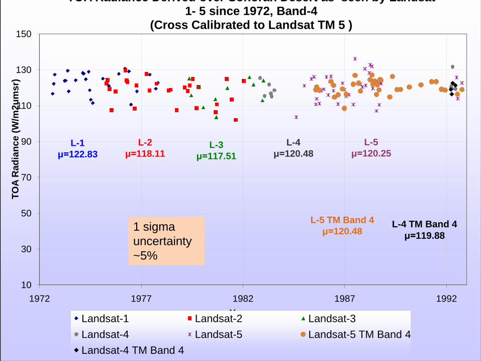
TOA Radiance Derived over Sonoran Desert as seen by Landsat 1- 5 since 1972, Band-4

(Cross Calibrated to Landsat TM 5 )

Landsat-1 Landsat-2 Landsat-3Landsat-4 Landsat-5 Landsat-5 TM Band 4Landsat-4 TM Band 4

L-1μ=122.83

L-2μ=118.11

L-3μ=117.51

L-4μ=120.48

L-5μ=120.25

L-5 TM Band 4μ=120.48

L-4 TM Band 4μ=119.88

1 sigma uncertainty ~5%

Validation By Completing the TM-MSS Love Loop(Converting TM 5 Radiance data to MSS 4 Radiance data)

TM 5

MSS 5 TM 4

MSS 4

GTM5-TM4

GTM4-MSS4X SBAFL4

GTM5-MSS5X SBAFL5

GMSS5-MSS4

Ben Jasinski

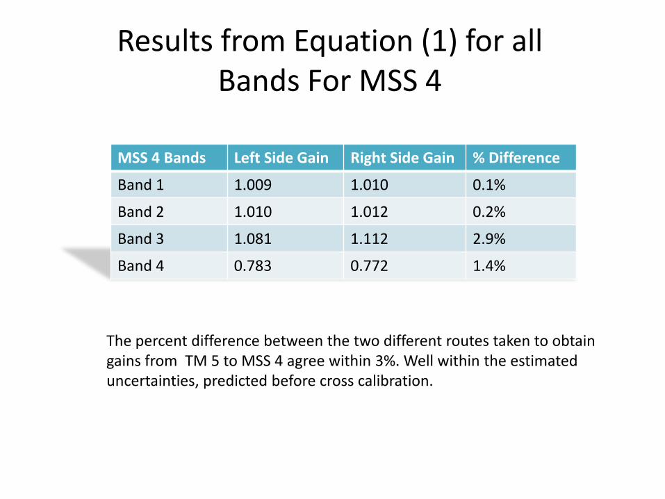
Results from Equation (1) for all Bands For MSS 4

MSS 4 Bands Left Side Gain Right Side Gain % Difference

Band 1 1.009 1.010 0.1%

Band 2 1.010 1.012 0.2%

Band 3 1.081 1.112 2.9%

Band 4 0.783 0.772 1.4%

The percent difference between the two different routes taken to obtain gains from TM 5 to MSS 4 agree within 3%. Well within the estimated uncertainties, predicted before cross calibration.

Absolute Gain and Bias for placing all Landsat Sensors on a

consistent absolute radiance scale

TM 5

TM 4

MSS 5

MSS 4

MSS 3

MSS 2

MSS 1

ETM+

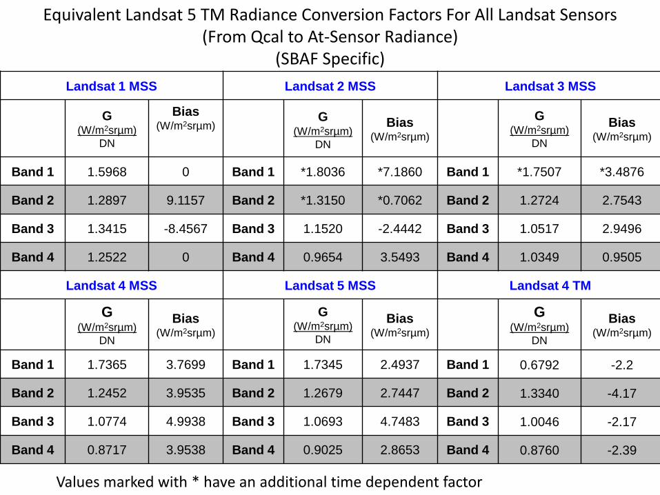
Equivalent Landsat 5 TM Radiance Conversion Factors For All Landsat Sensors(From Qcal to At-Sensor Radiance)

(SBAF Specific)Landsat 1 MSS Landsat 2 MSS Landsat 3 MSS

G (W/m2srµm)

DN

Bias(W/m2srµm)

G(W/m2srµm)

DN

Bias(W/m2srµm)

G (W/m2srµm)

DN

Bias(W/m2srµm)

Band 1 1.5968 0 Band 1 *1.8036 *7.1860 Band 1 *1.7507 *3.4876

Band 2 1.2897 9.1157 Band 2 *1.3150 *0.7062 Band 2 1.2724 2.7543

Band 3 1.3415 -8.4567 Band 3 1.1520 -2.4442 Band 3 1.0517 2.9496

Band 4 1.2522 0 Band 4 0.9654 3.5493 Band 4 1.0349 0.9505

Landsat 4 MSS Landsat 5 MSS Landsat 4 TM

G (W/m2srµm)

DN

Bias(W/m2srµm)

G (W/m2srµm)

DN

Bias(W/m2srµm)

G (W/m2srµm)

DN

Bias(W/m2srµm)

Band 1 1.7365 3.7699 Band 1 1.7345 2.4937 Band 1 0.6792 -2.2

Band 2 1.2452 3.9535 Band 2 1.2679 2.7447 Band 2 1.3340 -4.17

Band 3 1.0774 4.9938 Band 3 1.0693 4.7483 Band 3 1.0046 -2.17

Band 4 0.8717 3.9538 Band 4 0.9025 2.8653 Band 4 0.8760 -2.39

Values marked with * have an additional time dependent factor

Time Dependent Factor

Landsat 2 MSS

Time Dependent Factor

Band 1

Band 2

Landsat 3 MSS

Band 1

)85.144)(*56709.0(72.147

+− LaunchTT

)11.168)(*53916.0(85.170

+− LaunchTT

)10.144)(*5251.1(55.151

+− LaunchTT

Multiply the Gain and the Bias by the Time Dependent Factor

SUMMARY• Landsat Image Assessment System (IAS)

invaluable for continuous improvement of sensor calibration– Landsat 5 TM Relative Gains is a good example

• MTF Compensation is now a Landsat reality– Success with L4 TM Band 2 detectors may

suggest additional opportunities for improvements• A consistent absolute radiometric calibration

of Landsat sensors has been accomplished– At least in the desert…