ARTICLE

Recent increases in terrestrial carbon uptake atlittle cost to the water cycleLei Cheng1, Lu Zhang1, Ying-Ping Wang2, Josep G. Canadell 3, Francis H.S. Chiew1, Jason Beringer4,

Longhui Li5, Diego G. Miralles 6, Shilong Piao7,8,9 & Yongqiang Zhang 1

Quantifying the responses of the coupled carbon and water cycles to current global warming

and rising atmospheric CO2 concentration is crucial for predicting and adapting to climate

changes. Here we show that terrestrial carbon uptake (i.e. gross primary production)

increased significantly from 1982 to 2011 using a combination of ground-based and remotely

sensed land and atmospheric observations. Importantly, we find that the terrestrial

carbon uptake increase is not accompanied by a proportional increase in water use (i.e.

evapotranspiration) but is largely (about 90%) driven by increased carbon uptake per unit of

water use, i.e. water use efficiency. The increased water use efficiency is positively related to

rising CO2 concentration and increased canopy leaf area index, and negatively influenced

by increased vapour pressure deficits. Our findings suggest that rising atmospheric CO2

concentration has caused a shift in terrestrial water economics of carbon uptake.

DOI: 10.1038/s41467-017-00114-5 OPEN

1 CSIRO Land and Water, Black Mountain, Canberra, ACT 2601, Australia. 2 CSIRO Oceans and Atmosphere, PMB #1, Aspendale, VIC 3195, Australia.3 Global Carbon Project, CSIRO Oceans and Atmosphere, GPO Box 3023, Canberra, ACT 2601, Australia. 4 School of Agriculture and Environment, TheUniversity of Western Australia, Perth, WA 6009, Australia. 5 School of Life Sciences, University of Technology Sydney, Ultimo, NSW 2007, Australia.6 Laboratory of Hydrology and Water Management, Ghent University, Ghent 9000, Belgium. 7 Sino-French Institute for Earth System Science, College ofUrban and Environmental Sciences, Peking University, Beijing 100871, China. 8 Key Laboratory of Alpine Ecology and Biodiversity, Institute of Tibetan PlateauResearch, Chinese Academy of Sciences, Beijing 100085, China. 9 Center for Excellence in Tibetan Earth Science, Chinese Academy of Sciences,Beijing 100085, China. Correspondence and requests for materials should be addressed to L.C. (email: Lu.Zhang@CSIRO.au)

NATURE COMMUNICATIONS |8: 110 |DOI: 10.1038/s41467-017-00114-5 |www.nature.com/naturecommunications 1

G lobal warming, caused mainly by rising atmospheric CO2

concentration (Ca), is expected to accelerate theglobal water cycle1 and reduce terrestrial uptake of CO2

(i.e. gross primary production, GPP)2, 3. At the same time, risingCa has significant fertilization effects4 by enhancing terrestrialuptake of CO2 and by increasing ecosystem water use efficiency(WUE)5–8, i.e. the carbon uptake per unit of water loss(evapotranspiration, E), which in turn may affect the hydrologicalcycle9–11. Therefore, quantification of the responses of the waterand carbon cycles—which are closely coupled because photo-synthetic carbon uptake and transpiration both diffuse throughleaf stomata—to global warming and rising Ca is complex. Thereis still no consensus on how the coupled water and carbon cycleswill be altered under global environmental changes, especiallyunder rising Ca conditions9–15, yet quantification of suchcarbon–water changes is crucial to our predictive capability offuture climate change13, 16, water availability9, 10, 17, foodproduction and the ability to manage the biosphere for climatemitigation and adaptation18, 19.

Ecosystem WUE, or the carbon uptake (GPP) per unit of waterloss by ecosystem (E), is one of the most important ecosystemfunctional properties in driving terrestrial carbon and waterexchanges with the atmosphere5, 6, 20. Theory of leaf WUE,defined as leaf photosynthetic carbon uptake per unit of waterloss via transpiration, is relatively advanced, and various analy-tical models can explain variations of leaf WUE with plantfunction types and climate including those based on the opti-mization theory21, 22. However, understanding of WUE at theecosystem scale and global levels, defined as GPP per unit eco-system water loss via E, is still very limited6, 14, 20, 23–25. This isbecause other factors, such as soil, forest demography, nutrientsand atmospheric feedbacks, come into play to influence ecosys-tem carbon uptake, water use or both1, 10, 14. At present, analysisof ecosystem WUE at regional or global scale usually relies oncomplex land surface models (LSM) to estimate GPP and E inprior14, 23, both of which are associated with many poorlyquantified interactions across different spatiotemporal scales14, 26.Ecosystem GPP at large spatial and temporal scales is unobser-vable and is not well constrained25, 27–29. On the contrary,ecosystem water use, i.e. E, can be better constrained with widelyavailable hydrological observations (including precipitationand streamflow) at catchment, regional and global scales, wheredirect measurements of E are not available.

Here we develop a new WUE model independently from GPPand E, thus providing a robust alternative to existing WUEproducts, which in turn enables us to estimate GPP constrainedwith hydrological measurements. The new analytical WUE modelfor global terrestrial ecosystems is developed by upscaling leafWUE directly. Our model takes into account the controls ofatmospheric vapour pressure deficit (D), Ca and physiologicalfunctioning on leaf WUE. It also partitions among three differentcomponents of ecosystem water use through leaf area index (L)and the ratio of interception to total water use, i.e. fEi (seeMethods). The control of physiological functioning on leaf WUEis accounted for via parameter g1, which is a physiologicalparameter related to the functioning and response of stomatalconductance to environmental changes22, 30. Unlike previousstudies on WUE (e.g. refs. 6, 20, 23), this analytical model upscalesWUE from leaf to ecosystem directly and reduces uncertaintyconsiderably by not requiring prior estimates of GPP and E. Thus,hydrological estimates of ecosystem water use (i.e. E) are thenused to constrain the estimate of global GPP by multiplying WUEand E (denoted as WEC method, see Methods). Trends in theestimate of global WUE and GPP can then be attributed to dif-ferent drivers analytically. By combining multiple ground-basedand remotely sensed land and atmospheric observations into our

method, here we show that terrestrial GPP increased by 0.83±0.26 Pg C per year2 from 1982 to 2011. Importantly, we find thatthe GPP increase takes place at no cost of a significant increase inE, but is largely (about 90%) driven by the increased WUE, which,in turn, is driven by rising Ca and enhanced L.

ResultsThe validity of the analytical WUE model. The validity of theanalytical WUE model is supported by observed ecosystem WUEfrom eddy covariance sites (see Methods and SupplementaryTable 3). The linear correlation between observed and estimatedecosystem WUE of 229 site-years is about 0.64, with a relativebias of −10.6% and mean error of −0.26 g Cmm−1 H2O (Fig. 1a).The slope of the regressed line between observed and estimatedannual WUE passing through the origin is 0.84, with an adjustedR2 of 0.87. Across 11 sites with more than 6 years of continuousobservations, the estimated mean trend in ecosystem WUE isabout 14.7± 9.0 mg Cmm−1 H2O per year (mean± 1 standarderror), which is consistent with the in situ observed mean trend of12.6± 11.4 mg Cmm−1 H2O per year and with previousfindings23. The linear correlation coefficient between observedand estimated trends in annual WUE is about 0.93, with a relativebias of 17.2% and mean error of 2.16 mg Cmm−1 H2O per year(Fig. 1b). The slope of the regressed line between observed andestimated annual WUE passing through the origin is 0.78, with anadjusted R2 of 0.85.

We also assess the validity of our analytic model at the globalscale by comparing the estimated global mean and spatialvariation of ecosystem WUE with other independent estimates.To account for input uncertainties, we used 10 different ground-based and remotely sensed observations of global land andatmospheric forcing, and obtained an ensemble of 12 estimates ofglobal WUE with a spatial resolution of 0.5° by 0.5° (see Methods).We estimate the mean annual global WUE of 12 estimates to be2.1± 0.35 g Cmm−1 H2O (mean± 1 standard deviation, hereafterthe uncertainty is expressed as 1 standard deviation unlessspecified) from 1982 to 2011. Our global mean annual estimate isclose to, but about 20% larger than, the ensemble mean of the sixLSMs (Supplementary Table 4) of 1.66± 0.26 g Cmm−1 H2O, andthe independent estimates using the model tree ensemble (MTE)data set31 of 1.66± 0.02 g Cmm−1 H2O. Our estimated WUEshows distinctly spatial and latitudinal patterns (Fig. 1c), with lowvalues in the arid regions and high values in the tropical andboreal forests. Along different latitudes, it is relatively high inthe northern high latitude around 60°N and in the tropical regionaround 3°S. This spatial pattern of estimated global WUE is alsoconsistent with other independent estimates (see SupplementaryFig. 4).

Estimated global GPP. Based on the 12 annual WUE estimatesand 7 independent E products (see Methods and SupplementaryTable 2), we obtain an ensemble of 84 estimates of globalannual GPP from 1982 to 2011 by multiplying WUE and E (WECmethod, see Methods). The estimated mean annual global GPP of84 estimates is 146.1± 21.3 Pg C per year, and falls within thereported range of global GPP from 90 to 210 Pg C per year27, 29,32. The spatial details of our GPP estimates accord well withestimates derived using the MTE method or LSMs at the globalscale (Supplementary Fig. 5). This provides further confidencethat the new WUE model represents a robust and quantitativemeasure of the functional coupling between the terrestrial waterand carbon cycles, specifically GPP and E, allowing the use ofhydrological observations to constrain GPP estimates andexplaining the causality of the estimated trends in GPP over therecent years.

ARTICLE NATURE COMMUNICATIONS | DOI: 10.1038/s41467-017-00114-5

2 NATURE COMMUNICATIONS |8: 110 |DOI: 10.1038/s41467-017-00114-5 |www.nature.com/naturecommunications

Trends in global GPP and WUE and their attribution. Usingthe full ensemble of estimates (n= 84), we estimate that globalGPP has increased 0.83± 0.26 Pg C per year2 from 1982 to 2011on average (Fig. 2a, c, p< 0.001), or 7.33± 2.09 g Cm−2 per year2,or 0.6± 0.2% per year of mean annual GPP. By excluding one Lproduct that with systemic inconsistency in some regions(see Discussion), our best estimate of the trend in global GPP,based on an ensemble of 42 estimates, is 0.59± 0.12 Pg C peryear2 (0.33–0.87 Pg C per year2).

The range of the estimated trend in global GPP over1982–2011 by the WEC method is 0.33–1.30 Pg C per year2,

which is much wider than that derived from the sixLSMs (0.32–0.57 Pg C per year2). Reported values in other studiesgive a range from 0.2 to 0.66 Pg C per year2 (see refs. 28, 33, 34).The estimated trend in global GPP from all the 84 GPP estimatesis larger than the ensemble of 6 LSMs (0.44± 0.08 Pg C per year2)over the same period. However, our best estimate of 0.59± 0.12Pg C per year2 (n= 42) is quite close to the LSMs mean ensemble.

All seven E data sets show small trends over 1982−2011with one being negative, two being not significantlydifferent from zero (p> 0.05) and other four being significantlypositive (p< 0.05, see Supplementary Fig. 3). The mean trend of

0

1

1

2

2

3

3

4

4

5

5

6

60 0Observed annual WUE

Est

imat

ed a

nnua

l WU

Eg

C m

m−

1 H

2O−80

−40

0

40

80

−80 −40 40 80Observed trend in annual WUE

Est

imat

ed tr

end

in a

nnua

l WU

Em

g C

mm

−1

H2O

yea

r−1

−60

−40

−20

0

20

40

60

80

−180 −150 −120 −90 −60 −30 0 30 60 90 120 150 180

Latit

ude

(N)

Latit

ude

(N)

Mean annual WUE (g C mm−1 H2O)

0.50 0.75 1.00 1.25 1.50 1.75 2.00 2.25 2.50 2.75 3.00 3.25 3.50 4.00

−60

−40

−20

0

20

40

60

80

Mean annual GPP (g C m−2 year−1)

100 200 300 400 600 800 1000 1250 1500 1750 2000 2250 2500 2750 3000 3500

0

10

20

Obs

erve

d

Est

imat

ed

Longitude (E)

−180 −150 −120 −90 −60 −30 0 30 60 90 120 150 180Longitude (E)

a b

c

d

Fig. 1 Validation of the ecosystem water use efficiency (WUE) model and spatial variability of estimated mean annual WUE and gross primary production(GPP) over the period of 1982–2011. a Validation of annual WUE in g Cmm−1 H2O using observations from 51 eddy covariance flux sites (n= 229 site-years). The red line is the 1:1 line and blue line is fitted using least square regression. b Validation of the trends in annual WUE in mg Cmm−1 H2O per year at11 eddy covariance flux sites with at least 7 years observations. The red line is the 1:1 line. The error bars indicate one standard deviation of estimated andobserved trends using different methods. The inset shows the mean of observed and estimated trends of all the 11 stations. c, d Estimated spatial details(0.5° × 0.5°) of the global mean annual ecosystem WUE in g Cmm−1 H2O and gross primary production (GPP) in g Cm−2 per year, respectively, with bareland coloured in grey

NATURE COMMUNICATIONS | DOI: 10.1038/s41467-017-00114-5 ARTICLE

NATURE COMMUNICATIONS |8: 110 |DOI: 10.1038/s41467-017-00114-5 |www.nature.com/naturecommunications 3

all the seven E data sets is 0.37± 0.80 (range from −1.1 to 1.8)mm per year2, or 0.06± 0.13% per year of mean annual E.We estimate global ecosystem WUE has increased at a mean rateof 13.7± 4.3 mg Cmm−1 H2O per year from 1982 to 2011(Fig. 2b, d, p< 0.001), which is about 0.7± 0.2% per year of meanannual WUE.

The two drivers (E and WUE) contributing to the trends interrestrial GPP are further investigated (see Methods) and shownin Fig. 2c. Globally, both E and WUE positively contribute to theestimated increase in GPP. The contribution of WUE tothe estimated GPP trend is about 0.75± 0.25 Pg C per year2

or 90± 30% of the total GPP trend, as compared to about0.09± 0.12 Pg C per year2 or 10± 15% of the total GPP trend byE. The results suggest that estimated increase in global GPP underclimate change and rising Ca conditions over the past 30 years istaking place at no cost of using proportionally more water, but itis largely driven by the increase in carbon uptake per unit of wateruse, i.e. WUE.

Contributions of the four different variables (i.e. Ca, D, L andfEi ) to the estimated trend in WUE are further analysed(see Methods) and shown in Fig. 2d. Three of the four variables(except fEi ) have significant (p< 0.01) contributions tothe estimated increasing trend in global WUE, of which Ca andL have positive contributions but D has a negative contribution tothe estimated increase in WUE. The contributions of Ca, D, L andfEi to the estimated trend in global WUE are 9.9± 1.7, −3.4± 1.1,7.4± 4.3 and 0.04± 0.4 mg Cmm−1 H2O per year, or 77± 20%,−27± 11%, 49± 16% and 0.2± 3%, respectively. The contribu-tions of four drivers of WUE (i.e. Ca, D, L and fEi ) to the estimated

global GPP trends are 0.53± 0.06, −0.18± 0.04, 0.41± 0.24 and0.003± 0.02 Pg C per year2, or 64± 7%, −21± 5%, 49± 29%and 0.3± 3%, respectively. Therefore, recent changes in Ca, D andL are not only the main drivers of the estimated global WUEtrend, but also estimated global GPP trend.

Spatial variability of the estimated GPP and WUE trends.Spatially the trends of estimated GPP and WUE over the periodof 1982−2011 are quite variable (Fig. 3). The GPP trend variesfrom −4.4 to 27.2 g Cm−2 per year2 (1−99% range, Fig. 3a).Despite the large-scale occurrence of droughts and disturbancesover the study period35, remarkably, about 82± 5% of vegetatedland shows positive trends in GPP, of which about 80± 8% of thetrends is significant (p< 0.05). About 55± 11% of vegetated areasshow positive trends in E, of which only about 47± 4% issignificant (p< 0.05). Changes in WUE range from less than−6.6 to 51.3 mg Cmm−1 H2O per year (1−99% range, Fig. 3b). Anincrease in ecosystem WUE is found in 90± 2% ofvegetated areas over 1982–2011, of which about 78± 8% issignificant (p< 0.05). The remaining 10± 2% of the vegetatedland shows a decreasing trend, of which only about 21± 7% issignificant (p< 0.05).

Generally, spatial patterns of GPP and WUE trends are similar(Fig. 3a, b), which further supports that WUE is the dominantcontributor to the estimated GPP trend in most regions. Regionswith large increases in GPP and WUE are mainly in boreal andtropical forests. Negative trends in both WUE and GPP are foundonly over small areas in northeast China and Mongolia, and theinland of Australia. Central Africa experienced a decrease in GPP

−15

−10

−5

0

5

10

15

20

Glo

bal G

PP

ano

mal

ies

Pg

C y

ear−

1

−0.3

−0.2

−0.1

0.0

0.1

0.2

0.3

1980 1985 1990 1995 2000 2005 2010

Glo

bal W

UE

ano

mal

ies

g C

mm

−1 H

2O

−0.3

0.0

0.3

0.6

0.9

1.2

Total E WUE

Glo

bal G

PP

tren

dsP

g C

yea

r−2

−5

0

5

10

15

20

Total Ca D L fEi

Glo

bal W

UE

tren

dsm

g C

mm

−1 H

2O y

ear−

1

Year

a

b

c d

Fig. 2 Estimated trends in global gross primary production (GPP) and water use efficiency (WUE) and their drivers over 1982–2011. a, b Annual meananomalies and its standard deviation (shown as error bars) of global GPP in Pg C per year (n= 84) and global WUE in g Cmm−1 H2O (n= 12) during1982–2011, respectively. The green line in a and blue line in b represent the linear trend over the past three decades. c Contribution of E and WUE to totalglobal trends in GPP (Total). d Contributions of four factors to the total increase in global WUE (Total). Ca, D, L and f Ei

refer to contributions fromatmospheric CO2 concentration, vapour pressure deficit, leaf area index and fraction of canopy interception to total ecosystem water use, respectively.The error bars in all the subplots represent one standard deviation

ARTICLE NATURE COMMUNICATIONS | DOI: 10.1038/s41467-017-00114-5

4 NATURE COMMUNICATIONS |8: 110 |DOI: 10.1038/s41467-017-00114-5 |www.nature.com/naturecommunications

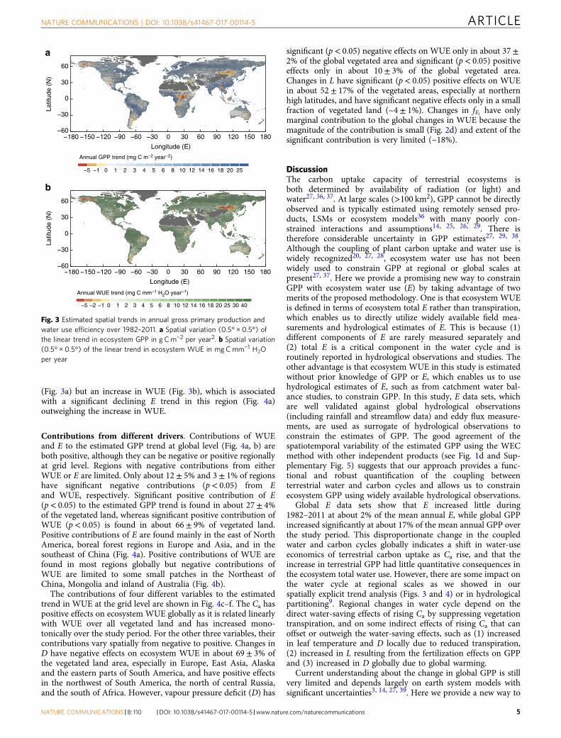
(Fig. 3a) but an increase in WUE (Fig. 3b), which is associatedwith a significant declining E trend in this region (Fig. 4a)outweighing the increase in WUE.

Contributions from different drivers. Contributions of WUEand E to the estimated GPP trend at global level (Fig. 4a, b) areboth positive, although they can be negative or positive regionallyat grid level. Regions with negative contributions from eitherWUE or E are limited. Only about 12± 5% and 3± 1% of regionshave significant negative contributions (p< 0.05) from Eand WUE, respectively. Significant positive contribution of E(p< 0.05) to the estimated GPP trend is found in about 27± 4%of the vegetated land, whereas significant positive contribution ofWUE (p< 0.05) is found in about 66± 9% of vegetated land.Positive contributions of E are found mainly in the east of NorthAmerica, boreal forest regions in Europe and Asia, and in thesoutheast of China (Fig. 4a). Positive contributions of WUE arefound in most regions globally but negative contributions ofWUE are limited to some small patches in the Northeast ofChina, Mongolia and inland of Australia (Fig. 4b).

The contributions of four different variables to the estimatedtrend in WUE at the grid level are shown in Fig. 4c–f. The Ca haspositive effects on ecosystem WUE globally as it is related linearlywith WUE over all vegetated land and has increased mono-tonically over the study period. For the other three variables, theircontributions vary spatially from negative to positive. Changes inD have negative effects on ecosystem WUE in about 69± 3% ofthe vegetated land area, especially in Europe, East Asia, Alaskaand the eastern parts of South America, and have positive effectsin the northwest of South America, the north of central Russia,and the south of Africa. However, vapour pressure deficit (D) has

significant (p< 0.05) negative effects on WUE only in about 37±2% of the global vegetated area and significant (p< 0.05) positiveeffects only in about 10± 3% of the global vegetated area.Changes in L have significant (p< 0.05) positive effects on WUEin about 52± 17% of the vegetated areas, especially at northernhigh latitudes, and have significant negative effects only in a smallfraction of vegetated land (~4± 1%). Changes in fEi have onlymarginal contribution to the global changes in WUE because themagnitude of the contribution is small (Fig. 2d) and extent of thesignificant contribution is very limited (~18%).

DiscussionThe carbon uptake capacity of terrestrial ecosystems isboth determined by availability of radiation (or light) andwater27, 36, 37. At large scales (>100 km2), GPP cannot be directlyobserved and is typically estimated using remotely sensed pro-ducts, LSMs or ecosystem models36 with many poorly con-strained interactions and assumptions14, 25, 26, 29. There istherefore considerable uncertainty in GPP estimates27, 29, 38.Although the coupling of plant carbon uptake and water use iswidely recognized20, 27, 28, ecosystem water use has not beenwidely used to constrain GPP at regional or global scales atpresent27, 37. Here we provide a promising new way to constrainGPP with ecosystem water use (E) by taking advantage of twomerits of the proposed methodology. One is that ecosystem WUEis defined in terms of ecosystem total E rather than transpiration,which enables us to directly utilize widely available field mea-surements and hydrological estimates of E. This is because (1)different components of E are rarely measured separately and(2) total E is a critical component in the water cycle and isroutinely reported in hydrological observations and studies. Theother advantage is that ecosystem WUE in this study is estimatedwithout prior knowledge of GPP or E, which enables us to usehydrological estimates of E, such as from catchment water bal-ance studies, to constrain GPP. In this study, E data sets, whichare well validated against global hydrological observations(including rainfall and streamflow data) and eddy flux measure-ments, are used as surrogate of hydrological observations toconstrain the estimates of GPP. The good agreement of thespatiotemporal variability of the estimated GPP using the WECmethod with other independent products (see Fig. 1d and Sup-plementary Fig. 5) suggests that our approach provides a func-tional and robust quantification of the coupling betweenterrestrial water and carbon cycles and allows us to constrainecosystem GPP using widely available hydrological observations.

Global E data sets show that E increased little during1982–2011 at about 2% of the mean annual E, while global GPPincreased significantly at about 17% of the mean annual GPP overthe study period. This disproportionate change in the coupledwater and carbon cycles globally indicates a shift in water-useeconomics of terrestrial carbon uptake as Ca rise, and that theincrease in terrestrial GPP had little quantitative consequences inthe ecosystem total water use. However, there are some impact onthe water cycle at regional scales as we showed in ourspatially explicit trend analysis (Figs. 3 and 4) or in hydrologicalpartitioning9. Regional changes in water cycle depend on thedirect water-saving effects of rising Ca by suppressing vegetationtranspiration, and on some indirect effects of rising Ca that canoffset or outweigh the water-saving effects, such as (1) increasedin leaf temperature and D locally due to reduced transpiration,(2) increased in L resulting from the fertilization effects on GPPand (3) increased in D globally due to global warming.

Current understanding about the change in global GPP is stillvery limited and depends largely on earth system models withsignificant uncertainties3, 14, 27, 39. Here we provide a new way to

−60

−30

0

30

60

−180 −150 −120 −90 −60 −30 0 30 60 90 120 150 180

−5 −1 0 1 2 3 4 5 6 8 10 12 14 16 18 20 25

a

−60

−30

0

30

60

−5 −2 −1 0 1 2 3 4 5 6 8 10 12 14 16 18 20 25 30 40

b

Latit

ude

(N)

Latit

ude

(N)

Longitude (E)

−180 −150 −120 −90 −60 −30 0 30 60 90 120 150 180

Longitude (E)

Annual GPP trend (mg C m−2 year−2)

Annual WUE trend (mg C mm−1 H2O year−1)

Fig. 3 Estimated spatial trends in annual gross primary production andwater use efficiency over 1982–2011. a Spatial variation (0.5° × 0.5°) ofthe linear trend in ecosystem GPP in g Cm−2 per year2. b Spatial variation(0.5° × 0.5°) of the linear trend in ecosystem WUE in mg Cmm−1 H2Oper year

NATURE COMMUNICATIONS | DOI: 10.1038/s41467-017-00114-5 ARTICLE

NATURE COMMUNICATIONS |8: 110 |DOI: 10.1038/s41467-017-00114-5 |www.nature.com/naturecommunications 5

estimate changes in global GPP and our estimated global trend inGPP is comparable with that derived from LSMs and indepen-dent studies. Across different eco-regions, trends in GPP esti-mated by the WEC method agree well with those derived from sixLSMs in term of the positive changes. Mean trends from the WECmethods are close to those from the LSMs at different ecoregions(Supplementary Table 7 and Supplementary Fig. 6), except for thetemperate and boreal forests and Tundra regions, where the meantrends estimated using WEC method are larger than thosederived from LSMs (see Supplementary Discussion and Supple-mentary Fig. 7). Basically, current understanding about the trendsin GPP at different spatial scales (i.e. from site to regional andglobal scales) is still very uncertain. Although not a proof, ourfindings of a significant increase in global GPP are consistent withother studies and with evolution of the global carbon budget overthe past 30 years3, 12.

Spatially, an estimated large increase in GPP can be foundmainly in two regions, i.e. the boreal forest and tropical forestregions (Fig. 3a). The relative large GPP increase in the borealforest region results from positive contributions from both E(Fig. 4a) and WUE (Fig. 4b). In turn, positive contribution ofWUE in this region is mainly driven by rising Ca and enhancedcanopy L (Fig. 4c, e). For the tropical forest region, the large GPPincrease mainly results from the increase in WUE in this region,caused by rising Ca (Fig. 4c), which is consistent with increasedWUE trend derived from tropical tree growth rings7.

At the global scale, the most important driver for the increasesin GPP and WUE from 1982 to 2011 is rising Ca. Global GPPincreases at a rate of 17% per 10% increase in Ca. The rising Ca isthe largest contributor to the estimated trend in GPP andenhances GPP at a rate of about 8% per 10% increase in Ca, which

is larger than the observed effect on net primary production fromfree-air CO2 experiments about 5% per 10% increase in Ca

40, 41.The analytical model estimates that global WUE increases at arate of 14% per 10% increase in Ca, of which the largest con-tributor is Ca. This is consistent with estimated global WUE trendand its attributions from LSMs23 and with the sensitivity ofecosystem WUE to Ca obtained from eddy flux observations andlong-term tree ring records24. Furthermore, the rising Ca mayhave an overall bigger role in the global water and carbon cyclesthan we reported here as increases in L can also be attributed torising Ca

42, 43.After rising Ca, the change in L is the second largest

contributor to the estimated trends of GPP and WUE globally.The impact of change in L on GPP is only indirectly accountedfor in the data products of E and estimated WUE. The two Lproducts used in this study show an increasing trend in L in thepast three decades42. Increase in L can lead to a positive trend inE because ecosystems with a greater L typically have higherinterception and transpiration44, 45. Increase in L can have bothpositive and negative effects on ecosystem WUE in this study. Anincrease in L can increase ecosystem WUE by increasingtranspiration fraction of ecosystem water use, or can decreaseecosystem WUE by increasing canopy interception (see Meth-ods). On average, ecosystem WUE increases with L to about3 and then decreases with L at the global scale (SupplementaryFig. 8). In reality, however, the controls of L on ecosystem wateruse partitioning are more complex than the method we used inthis study46, 47. The changes in L caused by environmentalchanges are complex10, 42, 43, 48, which poses limits to the capacityfor LSMs and the analytical WUE model here to project changesin future water and carbon cycles given that all parameterize L as

a b−60

−30

0

30

60

Latit

ude

(N)

Latit

ude

(N)

Annual GPP trend (mg C m−2 year−2)

−5 −1 0 1 2 3 4 5 6 8 10 12 14 16 18 20 25

c

e

d

f−120 −60 0 60 120 −120 −60 0 60 120

−60

−30

0

30

60

−60

−30

0

30

60

Longitude (E)

−120 −60 0 60 120 −120 −60 0 60 120Longitude (E)

Annual WUE trend (mg C mm−1 H2O year−1)

−5 −2 −1 0 1 2 3 4 5 6 8 10 12 14 16 18 20 25 30 40

Fig. 4 Estimated spatial variations of the contributions to trends of ecosystem gross primary production (GPP) and water use efficiency (WUE) fromdifferent variables over 1982–2011. a, b Spatial details of the contributions to recent trend in GPP from ecosystem water use and WUE in g Cm−2 per year2,respectively. c–f Spatial details of the contributions to trends in ecosystem WUE atmospheric CO2 concentration c, vapour pressure deficit d, leaf areaindex e and fraction of canopy interception in mg Cmm−1 H2O per year f

ARTICLE NATURE COMMUNICATIONS | DOI: 10.1038/s41467-017-00114-5

6 NATURE COMMUNICATIONS |8: 110 |DOI: 10.1038/s41467-017-00114-5 |www.nature.com/naturecommunications

the major control of water, energy and carbon fluxes betweenvegetated land surface and atmosphere.

One major source of uncertainity in the estimated annualWUE and GPP comes from the input data sets. Uncertainties inthe magnitude of global annual GPP is largely sourced from thedifferences in D amongst three data sets and different magnitudesof global E between reanalysis and diagnostic products. Globalannual E from reanalysis data sets is typically much larger thanthat of diagnostic E data sets. Uncertainties in the global GPPtrend are primarily sourced from different trends in E and Lproducts (Fig. 2c, d). The uncertainty in the contribution of E toglobal GPP trend (Fig. 2c) is largely resulted from two E data setsthat have very different trends from the other five E data sets. Theuncertainty in the contribution of L to global WUE (or GPP)trend results from a spurious step change around 2000 inone L product. Trends in global GPP from two L products are0.59± 0.12 and 1.06± 0.13 Pg C per year2, respectively. Thedifferences in D amongst three climate forcing data sets do notlead to significant uncertainty in the global WUE (or GPP) trends(Fig. 2d) as trends in D amongst three data sets agree with eachother well. In summary, differences amongst the input data setsdo not alter the estimated increasing trends in WUE and GPP atglobal scale (Fig. 2a, b), and therefore the conclusion of this study(see Supplementary Discussion).

The success of the developed analytical WUE model highlightsthe importance of the physiological parameter g1 for predictingthe functional and biogeographical variation in WUE, whichimplies that plant functional traits are very important to advanceour understanding about the coupled water and carbon cycles andtheir changes (also see refs. 25, 29). By directly accounting for keycontrols, our WUE model is analytically tractable, and lends itselfto identifying the major drivers of changes in ecosystem WUEwith quantifiable uncertainty. The ecosystem WUE model wehave developed uses a top-down approach49, 50 that provides ameaningful conceptualization of ecosystem WUE bydirectly accounting for key controls (or first-order controls) at theannual time scale and neglecting other factors that maybecome important at shorter (e.g. diurnal to seasonal) or longer(e.g. multiple decades to century) time scales includingdiurnal variations in meteorological conditions10, variable con-trols of L on E partitioning, long-term forest demography4 andnutrient limitations40, 51. Therefore, our model is best fitted forapplications at the annual to decadal time scales as a diagnostictool. The analytical WUE model captures satisfactorily the spatialand temporal variability of observed annual ecosystem WUE andproduces a global pattern of WUE consistent with other inde-pendent estimates. However, unexplained variability in ecosystemannual WUE and its trends by the proposed model is large at thesite level (Fig. 1a, b). Current available flux data are too limited toquantify the magnitude of trends in global WUE and GPP andthe associated uncertainty. There are 11 stations with longenough data for trend validation (Fig. 1b) covering seven differentplant function types based on our data-selection criteria. Thenumber of stations for every plant function types is no morethan 3. There is only one station located in the tropical forestregion and no station in the boreal forest regions for trend vali-dation. In addition, the estimated average trend in observedannual WUE has a large uncertainty (Fig. 1b) and is also muchlower than that reported by ref. 6. It reflects the fact that trends inecosystem WUE depend on the way it is defined and the studyregions and highlights that long-term observations available fordetecting changes in global water and carbon cycles are stilllimited, especially in the tropical and boreal forest regions wherewe find larger trends in WUE than in other regions. Therefore,further development and validation of the model are needed to

reliably interpret ecosystem WUE and its changes at annual andfiner spatiotemporal scales.

Our results show that terrestrial GPP has increasedsignificantly and is primarily associated with increase in WUE,which in turn is largely driven by rising Ca and increase in L.Little increase in E but significant increase in GPP suggests thatincrease in terrestrial carbon uptake over the past three decadeshas had little consequences in global ecosystem water use(but there can be significant changes at regional scale). Acrossdifferent regions, boreal and tropical forests increased theirecosystem WUE and annual GPP most significantly, with theincrease in L and Ca as the major drivers in boreal region and theincrease in Ca as the main driver in the tropical region.

MethodsThe analytical WUE model. In this study, the ecosystem WUE is defined asecosystem GPP per unit of ecosystem water loss via evapotranspiration (E), i.e.

WUE ¼ GPPE

ð1Þ

In Eq. (1), evapotranspiration, E, includes both productive water use, i.e. tran-spiration (Et), and non-productive water use, i.e. evaporation from soil surface (Es)and evaporation from canopy interception (Ei), namely,

E ¼ Et þ Es þ Ei ð2Þ

Productive water use, Et, is coupled to carbon assimilation as both CO2 and waterdiffuse through leaf stomata. However, non-productive water uses, i.e. Ei and Es,are only indirectly related to carbon productive processes. The role of non-productive water use on carbon production represents a major difference betweenleaf-scale and ecosystem-scale WUE. For growing season when GPP and Et aregreater than zero, then Eq. (1) can be reformulated as:

WUE ¼ GPPE

¼ GPPEt

EtEt þ Es

1� EiE

� �ð3Þ

Equation (3) states that growing season ecosystem WUE can be estimated as theproduct of three terms. The first is transpiration WUE, i.e. GPP/Et. The secondis partitioning between transpiration and soil evaporation during carbonassimilation period. The last term is one minus the fraction of interception to totalwater use, Ei/E (denoted as fEi ).

Previous studies have shown that leaf WUE is quite independent of the growthenvironment21 and can be directly scaled to canopy scale52, 53. Thus ecosystemtranspiration WUE, i.e. GPP/Et in Eq. (3), can be approximated by leaf WUE(WUEl) as in ref. 22:

GPPEt

¼RAdtRTdt

� WUEl ¼ AT¼ Capa

1:6 Dþ g1ffiffiffiffiD

p� � ð4Þ

where A is leaf net photosynthetic carbon uptake (µmol(CO2) m−2 s−1); T is leaftranspiration (µmol(H2O) m−2 s−1); Ca is ambient atmospheric CO2 concentrationin mol(CO2) mol−1(air); g1 is an empirical parameter of the Ball stomatalconductance model54 (kPa0.5); D is the vapour pressure deficit (kPa); and pa isatmospheric pressure (kPa). The stomatal conductance model used in Eq. (4) issimilar to the Ball–Berry stomatal conductance model that has been widely adoptedin most global land surface models. What is different is that parameters in Eq. (4)have meaningful ecological interpretations as stated in ref. 22; and were estimatedusing extensive field observations as provided in ref. 30.

Partitioning of transpiration and soil evaporation can be evaluated via Beer’sLaw as:

EtEt þ Es

¼ 1� exp �kLð Þ ð5Þ

where L is the canopy leaf area index, and k is the radiation extinction coefficient.Partitioning of transpiration and soil evaporation is much more complex thanBeer’s law in reality46, 47, especially at short times scales (i.e. hourly or diurnalscales). However, this study is focused on monthly to annual time scales, at whichBeer’s law can provide reasonable and accurate partitioning between transpirationand soil evaporation46, 55, 56.

Therefore, Eq. (3) for ecosystem WUE can be formulated as:

WUE ¼ Capa1:6 Dþ g1

ffiffiffiffiD

p� � 1� exp �kLð Þ½ � 1� fEið Þ ð6Þ

If the input of Ca in Eq. (6) is in ppm (1 ppm≈ 1 µmol(CO2) mol−1(air)),estimated WUE by Eq. (6) has a unit of µmol(CO2) mol−1(H2O). It canbe converted to g Cmm−1 H2O by a factor of about 0.667 × 10−3 (i.e.

NATURE COMMUNICATIONS | DOI: 10.1038/s41467-017-00114-5 ARTICLE

NATURE COMMUNICATIONS |8: 110 |DOI: 10.1038/s41467-017-00114-5 |www.nature.com/naturecommunications 7

1 µmol(CO2) mol−1(H2O)≈ 0.667 × 10−3 g C kg−1 H2O≈ 0.667 × 10−3 g Cmm−1

H2O).In this study, Eq. (6) is applied to annual time scale for identifying the major

drivers of changes in ecosystem WUE based on the readily available data only.Assuming that GPP and Es during the non-growing season is negligible, we useEq. (6) to estimate ecosystem annual WUE with the first two terms (i.e. Capa

1:6 Dþg1ffiffiffiD

pð Þand 1� exp �kLð Þ½ �) are estimated during growing season months only and thethird term (i.e. 1� fEið Þ) is estimated at an annual time scale, in which datarequirement of Eq. (6) is minimal and seasonal variations in ecosystem WUEare also preserved. We define the growing season as mean monthly air temperature>0 °C (Supplementary Fig. 1 and see Supplementary Discussion for more details).

Estimating global ecosystem WUE. Two parameters and five variables arerequired for estimating WUE according to Eq. (6). The two parameters are k andg1. The five variables are Ca, pa, D, L and fEi . Parameter k, the extinction coefficientof radiation, is set as a constant of 0.6 for all the vegetated land. Global map ofparameter g1 (Supplementary Fig. 2) is generated by interpolating g1 values ofdifferent plant functional types (Supplementary Table 1) adopted from ref. 30 witha global vegetation classification map (i.e. SYNMAP57). The data for variable Ca areobserved annual mean data at Mauna Loa site58 and accessed from NOAA’s EarthSystem Research Laboratory. Variable pa is a mean annual atmospheric pressurefield estimated from the monthly climatology data set developed by ClimaticResearch Unit (CRU)59. Three different inputs for variable D are used, which arederived from three global climate forcing data sets including the CRU-NCEPdata set59, the Princeton Global Forcing data60 and the WATCH Forcing DataERA-Interim (WFDEI) meteorological forcing data61. Two global leaf area indexdata sets, GIMMS-LAI3g62 and GLASS-LAI63, are used as input for variable L. Twodifferent global interception ratios for variable fEi are used, which are derived fromthe Global Land Evaporation Amsterdam Model (EGLEAM)64 and the CSIRO globalevapotranspiration data set (ECSIRO)45. All the spatial data are gridded to a spatialresolution of 0.5° using area weighted local area mean. This study focuses onlyon vegetated land cells that are defined as having a mean annual NormalizedDifference Vegetation Index >0.1 based on the GIMMS NDVI3g data set65.Based on 10 widely used atmospheric, land and remotely sensed observationsfor these five variables, 12 estimates of WUE are derived of an overlapping periodfrom 1982 to 2011.

Estimating global ecosystem GPP. Based on the analytical WUE model,ecosystem WUE and E are multiplied to estimate ecosystem carbon uptake(denoted as WEC method) as,

GPP ¼ WUE ´E ð7Þ

The proposed WEC model for estimating ecosystem GPP is based on theassumption that WUE is an ecosystem functional property that couples GPP and E.Therefore, ecosystem E data sets, which can be estimated from global observedhydrological observations, are used to constrain estimation of GPP.

In total, 84 estimates of global annual GPP are obtained by multiplying 12annual WUE estimates and 7 independent data sets of annual E (SupplementaryTable 2 and Supplementary Fig. 3). Global E data sets are used as a surrogate ofhydrological observations to constrain GPP estimation. Seven E data sets collectedincluding EMTE

31, 35, EGLEAM64, ECSIRO45, EWB-MTE66, EMERRAa

67, EMERRAs68, and

EERA69. The first four E data sets are diagnostic data sets, mostly based on in situand satellite remote sensing forcing, while the rest three are re-analysis data sets.The diagnostic E data sets have been widely validated against eddy fluxmeasurements and hydrological observations including precipitation andstreamflow data. The EMTE and EWB-MET are estimated using the MTE methodfrom global observed water fluxes at eddy flux sites31, 35 and streamflowobservations at catchment scale66, respectively. The EGLEAM and ECSIRO are thesame data sets used to derive the fEi , which are estimated from global multiplesatellite products and climate forcing data sets. The EMERRAa and EMERRAs areassimilation and land simulation data of the NASA’s Modern-Era RetrospectiveAnalysis for Research and Applications (MERRA) products67, 68, respectively.The EERA is the assimilation data of ERA-Interim product69.

Validation of the WUE model using eddy flux observations. The FLUX-NET2015 data set is applied to validate the analytical WUE model. The FLUX-NET2015 data set is the latest collection of global eddy flux observations, whichincludes sites of multiple regional flux networks and several improvements to thedata quality control protocols and data processing pipeline. After latest update onJuly of 2016, FLUXNET2015 has 165 stations globally with observations up to2014. All the monthly data of the 165 stations are collected firstly and someselection criteria are applied on some interested variables to screen data forvalidation.

Observed ecosystem annual WUE is estimated as the ratio of annual total GPP(in g Cm−2 per year) to total evapotranspiration (E in mm per year) according tothe definition of annual WUE in this study. Ecosystem annual GPP is estimated asthe average of different estimates of annual GPP in the FLUXNET2015 data setusing different methods partitioning of carbon flux (see http://fluxnet.fluxdata.org/data/fluxnet2015-dataset/data-processing/). Evapotranspiration is converted from

observed latent heat flux (LE) from unit of Wm−2 to the unit in equivalent depth ofwater in mm per year based on site observed monthly mean daily air temperature(Ta). We used corrected LE data for estimating ecosystem annual WUE. Correctionof LE is necessary as lack of energy closure is quite common in observed latentfluxes using eddy covariance techniques. The corrected LE data are provided in theFLUXNET2015 data set, which is based on the energy balance closure ratio andkeep the Bowen ratio unchanged.

Criteria applied to select GPP and corrected LE data for estimating observedannual WUE include: (1) based on the data quality information in theFLUXNET2015 data set, site-year with >80% of high-quality observed or gap-filleddata of hourly GPP and LE; (2) at least one pair of annual corrected LE andGPP are available; (3) energy closure bias is within 20%; (4) annual total GPP(in g Cm−2 per year) and LE (in mm per year) are >10; and (5) site is not irrigatedor wetlands. There are about 1180 site-years of data available in the FLUXNET2015data set, of which about 47% and 20% satisfies the first two and all five selectioncriteria, respectively.

The input data for estimate ecosystem annual WUE at flux sites are the same asthat for the global estimation. However, there is only one of the three collectedglobal climate forcing data set is up to 2014 (i.e. CRU-NCEP data set). The methodto estimate annual WUE at the site level using monthly data is the same as thatapplied at the global scale. To account the uncertainty in the estimated WUE,global leaf area index (L) and interception ratio (fEi ) data sets at its originalresolution and half degree resolution are used to estimate WUE at site level. At last,51 sites and 229 site-years data are selected for validating the analytical ecosystemWUE model considering both selection criteria and available of other variables forestimating site level WUE. The list of sites and their key information are providedin Supplementary Table 3.

The validity of the analytical ecosystem WUE model is assessed using all theobserved annual WUE, i.e. 229 station-years, and using annual trends of 11 siteswith minimum length of 7 years of observed data. Sites used for trend validationare also listed in Supplementary Table 3. The first validation can be considered as aspatial validation of capability of the model to produce the variability of WUEbetween-sites. The second validation can be considered as a temporal validation ofcapability of the model to reproduce observed inter-annual (between-years)variability. In addition, the proposed method for estimating GPP is also validated atthe site level and shown in Supplementary Fig. 9 (see Supplementary Discussion).

Validation of estimated global WUE and GPP. The spatial patterns andmagnitudes of estimated global WUE and GPP are compared against otherindependent estimates including one estimate using the MTE method31 andother six estimates by land surface models (Supplementary Table 4) of TRENDYmodelling experiments70.

Trend and its attribution. Trends in global WUE, E and GPP are estimated atboth global and grid levels using the Mann–Kendall non-parametric trend test withSen’s method, and significance levels on the basis of the Mann–Kendall tests.

The contributions of E and WUE to the total trend in GPP are isolated withthree modelling experiments. One is called real modelling experiment with all theinput data is the same as observed. The other two are control modellingexperiments, which fixed only one contributing variable (i.e. E or WUE) at theinitial condition in each modelling experiment. The trend of the differencesbetween the real and control experiments is considered as the contribution ofcontrolled variable to the total changes. Then, the contributions of E and WUE tototal trends are isolated. Similarly, contributions of four variables (i.e. Ca, L, D andfEi ) to the total trends in WUE are isolated with five modelling experiments.See Supplementary Tables 5 and 6 for more details.

Data availability. All data used in this study are obtained from the literature orpublically available databases, which can be found with the references provided inthe section of estimating of ecosystem WUE and GPP and also in SupplementaryTables 1–4.

Received: 30 June 2016 Accepted: 2 June 2017

References1. Huntington, T. G. Evidence for intensification of the global water cycle: review

and synthesis. J. Hydrol. 319, 83–95 (2006).2. Friedlingstein, P. et al. Positive feedback between future climate change and the

carbon cycle. Geophys. Res. Lett. 28, 1543–1546 (2001).3. Arora, V. K. et al. Carbon–concentration and carbon–climate feedbacks in

cmip5 earth system models. J. Clim. 26, 5289–5314 (2013).4. Körner, C., Morgan, J., & Norby, R. in Terrestrial Ecosystems in a Changing

World (eds Canadell, J. G. et al.), pp. 9–21 (Springer, 2007).

ARTICLE NATURE COMMUNICATIONS | DOI: 10.1038/s41467-017-00114-5

8 NATURE COMMUNICATIONS |8: 110 |DOI: 10.1038/s41467-017-00114-5 |www.nature.com/naturecommunications

5. Ainsworth, E. A. & Long, S. P. What have we learned from 15 years of free-airCO2 enrichment (FACE)? A meta-analytic review of the responses ofphotosynthesis, canopy properties and plant production to rising CO2.New Phytol. 165, 351–372 (2005).

6. Keenan, T. F. et al. Increase in forest water-use efficiency as atmospheric carbondioxide concentrations rise. Nature 499, 324–327 (2013).

7. van der Sleen, P. et al. No growth stimulation of tropical trees by 150 years ofCO2 fertilization but water-use efficiency increased. Nat. Geosci. 8, 24–28(2015).

8. Frank, D. C. et al. Water-use efficiency and transpiration across Europeanforests during the Anthropocene. Nat. Clim. Change 5, 579–583 (2015).

9. Gedney, N. et al. Detection of a direct carbon dioxide effect in continental riverrunoff records. Nature 439, 835–838 (2006).

10. Field, C. B., Jackson, R. B. & Mooney, H. A. Stomatal responses to increasedCO2: implications from the plant to the global scale. Plant Cell Environ. 18,1214–1225 (1995).

11. Huntington, T. G. CO2-induced suppression of transpiration cannot explainincreasing runoff. Hydrol. Process. 22, 311–314 (2008).

12. Le Quere, C. et al. Trends in the sources and sinks of carbon dioxide.Nat. Geosci. 2, 831–836 (2009).

13. Gregory, J. M., Jones, C. D., Cadule, P. & Friedlingstein, P. Quantifying carboncycle feedbacks. J. Clim. 22, 5232–5250 (2009).

14. Medlyn, B. E. et al. Using ecosystem experiments to improve vegetation models.Nat. Clim. Change 5, 528–534 (2015).

15. Piao, S. et al. Changes in climate and land use have a larger direct impact thanrising CO2 on global river runoff trends. Proc. Natl Acad. Sci. USA 104,15242–15247 (2007).

16. Ben, B. B. B. et al. High sensitivity of future global warming to land carboncycle processes. Environ. Res. Lett. 7, 024002 (2012).

17. Ukkola, A. M. et al. Reduced streamflow in water-stressed climates consistentwith CO2 effects on vegetation. Nat. Clim. Change 6, 75–78 (2016).

18. Canadell, J. G., & Schulze, E. D. Global potential of biospheric carbonmanagement for climate mitigation, Nat. Commun. 5, 5282 (2014).

19. Jackson, R. B. et al. Trading water for carbon with biological carbonsequestration. Science 310, 1944–1947 (2005).

20. Beer, C. et al. Temporal and among-site variability of inherent water useefficiency at the ecosystem level. Global Biogeochem. Cycles 23, GB2018 (2009).

21. Wong, S. C., Cowan, I. R. & Farquhar, G. D. Stomatal conductance correlateswith photosynthetic capacity. Nature 282, 424–426 (1979).

22. Medlyn, B. E. et al. Reconciling the optimal and empirical approaches tomodelling stomatal conductance. Global Change Biol. 17, 2134–2144 (2011).

23. Huang, M. et al. Change in terrestrial ecosystem water-use efficiency over thelast three decades. Global Change Biol. 21, 2366–2378 (2015).

24. Dekker, S. C., Groenendijk, M., Booth, B. B. B., Huntingford, C. & Cox, P. M.Spatial and temporal variations in plant water-use efficiency inferred from tree-ring, eddy covariance and atmospheric observations. Earth Syst. Dynam. 7,525–533 (2016).

25. Reichstein, M., Bahn, M., Mahecha, M. D., Kattge, J. & Baldocchi, D. D. Linkingplant and ecosystem functional biogeography. Proc. Natl Acad. Sci. USA 111,13697–13702 (2014).

26. Friedlingstein, P. et al. Uncertainties in CMIP5 climate projections due tocarbon cycle feedbacks. J. Clim. 27, 511–526 (2013).

27. Beer, C. et al. Terrestrial gross carbon dioxide uptake: global distribution andcovariation with climate. Science 329, 834–838 (2010).

28. Anav, A. et al. Spatiotemporal patterns of terrestrial gross primary production:a review. Rev. Geophys. 53, 785–818 (2015).

29. Wang, Y. P. et al. Correlations among leaf traits provide a significant constrainton the estimate of global gross primary production. Geophys. Res. Lett. 39,L19405 (2012).

30. Lin, Y. et al. Optimal stomatal behaviour around the world. Nat. Clim. Change5, 459–464 (2015).

31. Jung, M. et al. Global patterns of land-atmosphere fluxes of carbon dioxide,latent heat, and sensible heat derived from eddy covariance, satellite, andmeteorological observations. J. Geophys. Res. 116, G00J07 (2011).

32. Welp, L. R. et al. Interannual variability in the oxygen isotopes of atmosphericCO2 driven by El Nino. Nature 477, 579–582 (2011).

33. Anav, A. et al. Evaluating the land and ocean components of the global carboncycle in the CMIP5 earth system models. J. Clim. 26, 6801–6843 (2013).

34. Jiang, C. & Ryu, Y. Multi-scale evaluation of global gross primary productivityand evapotranspiration products derived from Breathing Earth SystemSimulator (BESS). Remote Sens. Environ. 186, 528–547 (2016).

35. Jung, M. et al. Recent decline in the global land evapotranspiration trend due tolimited moisture supply. Nature 467, 951–954 (2010).

36. Running, S. W. et al. A continuous satellite-derived measure of global terrestrialprimary production. BioScience 54, 547–560 (2004).

37. Beer, C., Reichstein, M., Ciais, P., Farquhar, G. D. & Papale, D. Mean annualGPP of Europe derived from its water balance. Geophys. Res. Lett. 34, L05401(2007).

38. Turner, D. P. et al. Evaluation of MODIS NPP and GPP products acrossmultiple biomes. Remote Sens. Environ. 102, 282–292 (2006).

39. Canadell, J. G. & Raupach, M. R. Managing forests for climate changemitigation. Science 320, 1456–1457 (2008).

40. Norby, R. J. et al. Forest response to elevated CO2 is conserved across abroad range of productivity. Proc. Natl Acad. Sci. USA 102, 18052–18056(2005).

41. Norby, R. J., Warren, J. M., Iversen, C. M., Medlyn, B. E. & McMurtrie, R. E.CO2 enhancement of forest productivity constrained by limited nitrogenavailability. Proc. Natl Acad. Sci. USA 107, 19368–19373 (2010).

42. Zhu, Z. et al. Greening of the Earth and its drivers. Nat. Clim. Change 6,791–795 (2016).

43. Donohue, R. J., Roderick, M. L., McVicar, T. R. & Farquhar, G. D. CO2

fertilisation has increased maximum foliage cover across the globe’s warm, aridenvironments. Geophys. Res. Lett. 12, 3031–3035 (2013).

44. Zhang, L., Dawes, W. R. & Walker, G. R. Response of mean annualevapotranspiration to vegetation changes at catchment scale.Water Resour. Res.37, 701–708 (2001).

45. Zhang, Y. et al. Multi-decadal trends in global terrestrial evapotranspirationand its components. Sci. Rep. 6, 19124 (2016).

46. Wang, L., Good, S. P. & Caylor, K. K. Global synthesis of vegetation control onevapotranspiration partitioning. Geophys. Res. Lett. 41, 6753–6757 (2014).

47. Jarvis, P. G., & McNaughton, K. G. Stomatal control of transpiration: scaling upfrom leaf to region. Adv. Ecol. Res. 15, 1–49 (1986).

48. Cowling, S. A. & Field, C. B. Environmental control of leaf area production:implications for vegetation and land-surface modeling. Global Biogeochem.Cycles 17, 1007 (2003).

49. Sivapalan, M., Blöschl, G., Zhang, L. & Vertessy, R. Downward approach tohydrological prediction. Hydrol. Process. 17, 2099 (2003).

50. Jarvis, P. G. in Scaling Physiological Processes: Leaf to Globe(eds Ehleringer, J. R. and Field, C. B.) (Academic Press, 1993).

51. Houlton, B. Z., Wang, Y., Vitousek, P. M. & Field, C. B. A unifyingframework for dinitrogen fixation in the terrestrial biosphere. Nature 454,327–330 (2008).

52. Wong, S. C. & Dunin, F. X. Photosynthesis and transpiration of trees in aeucalypt forest stand: CO2, light and humidity responses. Funct. Plant Biol. 14,619–632 (1987).

53. Barton, C. V. M. et al. Effects of elevated atmospheric [CO2] on instantaneoustranspiration efficiency at leaf and canopy scales in Eucalyptus saligna. GlobalChange Biol. 18, 585–595 (2012).

54. Ball, J. T., Woodrow, I. E., and Berry, J. A. A Model predicting stomatalconductance and its contribution to the control of photosynthesis underdifferent environmental conditions. In Progress in Photosynthesis Research(Ed. Biggins, J.) 221–224 (Springer 1987).

55. Schulze, E. D., Kelliher, F. M., Korner, C., Jon, L. & Leuning, R. Relationshipsamong maximum stomatal conductance, ecosystem surface conductance,carbon assimilation rate, and plant nitrogen nutrition: a global ecology scalingexercise. Ann. Rev. Ecol. Syst. 25, 629–660 (1994).

56. Kelliher, F. M., Leuning, R., Raupach, M. R. & Schulze, E. D. Maximumconductances for evaporation from global vegetation types. Agr. ForestMeteorol. 73, 1–16 (1995).

57. Jung, M., Henkel, K., Herold, M. & Churkina, G. Exploiting synergies of globalland cover products for carbon cycle modeling. Remote Sens. Environ. 101,534–553 (2006).

58. Keeling, C. D. et al. Atmospheric carbon dioxide variations at Mauna LoaObservatory. Hawaii, Tellus 28, 538–551 (1976).

59. New, M., Hulme, M. & Jones, P. Representing twentieth-century space–timeclimate variability. Part I: development of a 1961–90 mean monthly terrestrialclimatology. J. Clim. 12, 829–856 (1999).

60. Sheffield, J., Goteti, G. & Wood, E. F. Development of a 50-year high-resolutionglobal dataset of meteorological forcings for land surface modeling. J. Clim. 19,3088–3111 (2006).

61. Weedon, G. P. et al. The WFDEI meteorological forcing data set: WATCHforcing data methodology applied to ERA-Interim reanalysis data. WaterResour. Res. 50, 7505–7514 (2014).

62. Zhu, Z. et al. Global data sets of vegetation leaf area index (LAI)3g and fractionof photosynthetically active radiation (FPAR)3g derived from global inventorymodeling and mapping studies (GIMMS) normalized difference vegetationindex (NDVI3g) for the period 1981 to 2011. Remote Sens. 5, 927 (2013).

63. Liang, S., & Xiao, Z. Global Land Surface Products: Leaf Area Index ProductData Collection (1985-2010) (Beijing Normal University, 2012).

64. Miralles, D. G., De Jeu, R. A. M., Gash, J. H., Holmes, T. R. H. & Dolman, A. J.Magnitude and variability of land evaporation and its components at the globalscale. Hydrol. Earth Syst. Sci. 15, 967–981 (2011).

65. Pinzon, J. E. & Tucker, C. J. A non-stationary 1981–2012 AVHRR NDVI3gtime series. Remote Sens. 6, 6929–6960 (2014).

NATURE COMMUNICATIONS | DOI: 10.1038/s41467-017-00114-5 ARTICLE

NATURE COMMUNICATIONS |8: 110 |DOI: 10.1038/s41467-017-00114-5 |www.nature.com/naturecommunications 9

66. Zeng, Z. et al. A worldwide analysis of spatiotemporal changes in waterbalance-based evapotranspiration from 1982 to 2009. J. Geophys. Res. Atmos119, 1186–1202 (2014).

67. Rienecker, M. M. et al. MERRA: NASA's Modern-Era retrospective analysis forresearch and applications. J. Clim. 24, 3624–3648 (2011).

68. Reichle, R. H. et al. Assessment and enhancement of MERRA land surfacehydrology estimates. J. Clim. 24, 6322–6338 (2011).

69. Dee, D. P. et al. The ERA-Interim reanalysis: configuration and performance ofthe data assimilation system. Q. J. Roy. Meteor. Soc. 137, 553–597 (2011).

70. Sitch, S. et al. Recent trends and drivers of regional sources and sinks of carbondioxide,. Biogeosciences 12, 653–679 (2015).

AcknowledgementsL.C. thanks the support from CSIRO OCE post-doctoral research fellowship. L.Z. thanksthe support from CSIRO-CAS Climate Change Impacts Theme. Y.-P.W. thanks thefinancial support from CSIRO CABLE science project and from CSIRO strategic projectof global biogeochemistry and NESP. J.G.C. thanks the support of the EarthSystems Climate Change Hub of the Australian National Environmental ScienceProgram. J.B. acknowledges support from the ARC Future Fellowship (FT110100602).D.G.M. acknowledges support from the European Research Council (ERC) under grantagreement 715254 (DRY–2–DRY). We thank all people and institutions that providedata used in this study, in particular, the Max Planck Institute for Biogeochemistry andthe TRENDY modelling group. We are grateful to the research centres that made thesatellite and re-analysis data available, and especially to Dr. Zaichun Zhu, who shared thelatest version of GIMMS LAI3g data set. This work used eddy covariance data acquiredand shared by the FLUXNET community, including these networks: AmeriFlux,AfriFlux, AsiaFlux, CarboAfrica, CarboEuropeIP, CarboItaly, CarboMont, ChinaFlux,Fluxnet-Canada, GreenGrass, ICOS, KoFlux, LBA, NECC, OzFlux-TERN, TCOS-Siberiaand USCCC. The FLUXNET eddy covariance data processing and harmonization wascarried out by the ICOS Ecosystem Thematic Center, AmeriFlux Management Projectand Fluxdata project of FLUXNET, with the support of CDIAC, and the OzFlux,ChinaFlux and AsiaFlux offices.

Author contributionsL.Z., Y.-P.W., L.C., J.G.C. and F.H.S.C. designed the study. L.C. performed the analysis;L.C., L.Z., Y.-P.W., J.G.C. and F.H.S.C. drafted the paper. L.C., J.B., L.L., D.G.M., S.P. andY.Z. collected data and prepared figures. All authors contributed to the interpretation ofthe results and to the text.

Additional informationSupplementary Information accompanies this paper at doi:10.1038/s41467-017-00114-5.

Competing interests: The authors declare no competing financial interests.

Reprints and permission information is available online at http://npg.nature.com/reprintsandpermissions/

Publisher's note: Springer Nature remains neutral with regard to jurisdictional claims inpublished maps and institutional affiliations.

Open Access This article is licensed under a Creative CommonsAttribution 4.0 International License, which permits use, sharing,

adaptation, distribution and reproduction in any medium or format, as long as you giveappropriate credit to the original author(s) and the source, provide a link to the CreativeCommons license, and indicate if changes were made. The images or other third partymaterial in this article are included in the article’s Creative Commons license, unlessindicated otherwise in a credit line to the material. If material is not included in thearticle’s Creative Commons license and your intended use is not permitted by statutoryregulation or exceeds the permitted use, you will need to obtain permission directly fromthe copyright holder. To view a copy of this license, visit http://creativecommons.org/licenses/by/4.0/.

© The Author(s) 2017

ARTICLE NATURE COMMUNICATIONS | DOI: 10.1038/s41467-017-00114-5

10 NATURE COMMUNICATIONS |8: 110 |DOI: 10.1038/s41467-017-00114-5 |www.nature.com/naturecommunications