recent advances in applied probability · contents preface acknowledgments modeling text databases...

Recent Advances in Applied Probability

Recent Advances in Applied Probability

Edited by

RICARDO BAEZA-YATESUniversidad de Chile, Chile

JOSEPH GLAZUniversity of Connecticut, USA

HENRYK GZYLUniversidad Simón Bolívar, Venezuela

JÜRGEN HÜSLERUniversity of Bern, Switzerland

JOSÉ LUIS PALACIOSUniversidad Simón Bolívar, Venezuela

Springer

eBook ISBN: 0-387-23394-6Print ISBN: 0-387-23378-4

Print ©2005 Springer Science + Business Media, Inc.

All rights reserved

No part of this eBook may be reproduced or transmitted in any form or by any means, electronic,mechanical, recording, or otherwise, without written consent from the Publisher

Created in the United States of America

Boston

©2005 Springer Science + Business Media, Inc.

Visit Springer's eBookstore at: http://ebooks.kluweronline.comand the Springer Global Website Online at: http://www.springeronline.com

Contents

Preface

Acknowledgments

Modeling Text DatabasesRicardo Baeza-Yates, Gonzalo Navarro

1.11.21.31.41.51.61.7

IntroductionModeling a DocumentRelating the Heaps’ and Zipf’s LawModeling a Document CollectionModels for Queries and AnswersApplication: Inverted Files for the WebConcluding Remarks

AcknowledgmentsAppendix

References

An Overview of Probabilistic and Time Series Models in FinanceAlejandro Balbás, Rosario Romera, Esther Ruiz

2.12.22.32.42.5

IntroductionProbabilistic models for financeTime series modelsApplications of time series to financial modelsConclusions

References

Stereological estimation of the rose of directions from the rose of intersectionsViktor Beneš, Ivan Sax

3.13.2

An analytical approachConvex geometry approach

Acknowledgments

References

Approximations for Multiple Scan StatisticsJie Chen, Joseph Glaz

4.1 Introduction

xi

xiii

1

1378

101420

2121

24

27

2728384655

55

65

6673

95

95

97

97

vi RECENTS ADVANCES IN APPLIED PROBABILITY

4.24.34.44.5

The One Dimensional CaseThe Two Dimensional CaseNumerical ResultsConcluding Remarks

98

References

Krawtchouk polynomials and Krawtchouk matricesPhilip Feinsilver, Jerzy Kocik

5.15.25.35.45.55.65.7

What are Krawtchouk matricesKrawtchouk matrices from Hadamard matricesKrawtchouk matrices and symmetric tensorsEhrenfest urn modelKrawtchouk matrices and classical random walks“Kravchukiana” or the World of Krawtchouk PolynomialsAppendix

References

An Elementary Rigorous Introduction to Exact SamplingF. Friedrich, G. Winkler, O. Wittich, V. Liebscher

6.16.26.36.46.5

IntroductionExact SamplingMonotonicityRandom Fields and the Ising ModelConclusion

Acknowledgment

References

On the different extensions of the ergodic theorem of information theoryValerie Girardin

7.17.27.37.4

IntroductionBasicsThe theorem and its extensionsExplicit expressions of the entropy rate

References

101104106

113

115

115118122126129133137

140

143

144148157159160

161

161

163

163164170175

177

181

182183185186188191192192

Dynamic stochastic models for indexes and thesauri, identification clouds,and information retrieval and storage

Michiel Hazewinkel8.18.28.38.48.58.68.78.8

IntroductionA First Preliminary Model for the Growth of IndexesA Dynamic Stochastic Model for the Growth of IndexesIdentification CloudsApplication 1: Automatic Key Phrase AssignmentApplication 2: Dialogue Mediated Information RetrievalApplication 3: Distances in Information SpacesApplication 4: Disambiguation

Contents vii

8.98.108.118.128.138.148.158.168.178.188.198.20

Application 5. Slicing TextsWeightsApplication 6. SynonymsApplication 7. Crosslingual IRApplication 8. Automatic ClassificationApplication 9. Formula RecognitionContext Sensitive IRModels for ID CloudsAutomatic Generation of Identification CloudsMultiple Identification CloudsMore about Weights. Negative WeightsFurther Refinements and Issues

193194196196197197199199200200201202

203

205

205208

211

216

221

223

223226231233

238

241

241244252263

267

267

269

269271271

References

Stability and Optimal Control for Semi-Markov Jump ParameterLinear Systems

Kenneth J. Hochberg, Efraim Shmerling9.19.29.3

9.4

IntroductionStability conditions for semi-Markov systemsOptimization of continuous control systems with semi-Markov co-efficientsOptimization of discrete control systems with semi-Markov coeffi-cients

References

Statistical Distances Based on Euclidean GraphsR. Jiménez, J. E. Yukich

10.110.210.310.4

Introduction and backgroundThe nearest neighbor and main resultsStatistical distances based on Voronoi cellsThe objective method

References

Implied Volatility: Statics, Dynamics, and Probabilistic InterpretationRoger W. Lee

11.111.211.311.4

IntroductionProbabilistic InterpretationStaticsDynamics

Acknowledgments

References

On the Increments of the Brownian SheetJosé R. León, Oscar Rondón

12.112.212.3

IntroductionAssumptions and NotationsResults

viii RECENTS ADVANCES IN APPLIED PROBABILITY

12.4 ProofsAppendix

273277

278References

279

279282283286290292

296

296

299

299301303306311

313314317

326

326

329

329330333335336342346

348

351

351353361365

Compound Poisson Approximation with Drift for Stochastic AdditiveFunctionals with Markov and Semi-Markov Switching

Vladimir S. Korolyuk, Nikolaos Limnios13.113.213.313.413.513.6

IntroductionPreliminariesIncrement ProcessIncrement Process in an Asymptotic Split Phase SpaceContinuous Additive FunctionalScheme of Proofs

Acknowledgments

References

Penalized Model Selection for Ill-posed Linear ProblemsCarenneLudeña, Ricardo Ríos

14.114.214.314.414.5

14.614.714.8

IntroductionPenalized model selection [Barron, Birgé & Massart, 1999]Minimax estimation for ill posed problemsPenalized model selection for ill posed linear problemsBayesian interpretation

penalizationNumerical examplesAppendix

Acknowledgments

References

The Arov-Grossman Model and Burg’s EntropyJ.G. Marcano, M.D. Morán

15.115.215.315.415.515.615.7

IntroductionNotations and preliminariesLevinson’s Algorithm and Schur’s AlgorithmThe Christoffel-Darboux formulaDescription of all spectrums of a stationary processOn covariance’s extension problemBurg’s Entropy

References

Recent Results in Geometric Analysis Involving ProbabilityPatrick McDonald

16.116.216.316.4

IntroductionNotation and Background MaterialThe geometry of small balls and tubesSpectral Geometry

Contents ix

16.516.616.716.8

Isoperimetric Conditions and Comparison GeometryMinimal VarietiesHarmonic FunctionsHodge Theory

375382383388

391

397

398405406406412418422424

425

426

427

427430431433436441

452

455

455456458464472482490

491

491

495

References

Dependence or Independence of the Sample Mean and Variance In Non-IIDor Non-Normal Cases and the Role or Some Tests of Independence

Nitis Mukhopadhyay17.117.217.317.417.517.617.717.8

IntroductionA Multivariate Normal Probability ModelA Bivariate Normal Probability ModelBivariate Non-Normal Probability Models: Case IBivariate Non-Normal Probability Models: Case IIA Bivariate Non-Normal Population: Case IIIMultivariate Non-Normal Probability ModelsConcluding Thoughts

Acknowledgments

References

Optimal Stopping Problems for Time-Homogeneous Diffusions: a ReviewJesper Lund Pedersen

18.118.218.318.418.518.6

IntroductionFormulation of the problemExcessive and superharmonic functionsCharacterization of the value functionThe free-boundary problem and the principle of smooth fitExamples and applications

References

Criticality in epidemics:The mathematics of sandpiles explains uncertainty in epidemic outbreaks

Nico Stollenwerk19.119.219.319.419.519.619.7

IntroductionBasic epidemiological modelMeasles around criticalityMeningitis around criticalitySpatial stochastic epidemicsDirected percolation and path integralsSummary

Acknowledgments

References

Index

Preface

The possibility of the present collection of review papers came up the lastday of IWAP 2002. The idea was to gather in a single volume a sample of themany applications of probability.

As a glance at the table of contents shows, the range of covered topics iswide, but it sure is far away of being close to exhaustive.

Picking up a name for this collection not easier than deciding on a criterionfor ordering the different contributions. As the word ‘advances” suggests, eachpaper represents a further step toward understanding a class of problems. Nolast word on any problem is said, no subject is closed.

Even though there are some overlaps in subject matter, it does not seemsensible to order this eclectic collection except by chance, and such an orderis already implicit in a lexicographic ordering by first author’s last name: No-body (usually, that is) chooses a last name, does she/he? So that is how wesettled the matter of ordering the papers.

We thank the authors for their contribution to this volume.

We also thank John Martindale, Editor, Kluwer Academic Publishers, forinviting us to edit this volume and for providing continual support and encour-agement.

AcknowledgmentsThe editors thank the Cyted Foundation, Institute of Mathematical Statis-

tics, Latin American Regional Committee of the Bernoulli Society, NationalSecurity Agency and the University of Simon Bolivar for co-sponsoring IWAP2002 and for providing financial support for its participants.

The editors warmly thank Alfredo Marcano of Universidad Central de Ve-nezuela for having taken upon his shoulders the painstaking job of renderingthe different idiosyncratic contributions into a unified format.

MODELING TEXT DATABASES

Ricardo Baeza-YatesDepto. de Ciencias de la ComputaciónUniversidad de ChileCasilla 2777, Santiago, Chile

[email protected]

Gonzalo NavarroDepto. de Ciencias de la ComputaciónUniversidad de ChileCasilla 2777, Santiago, Chile

[email protected]

Abstract We present a unified view to models for text databases, proving new relationsbetween empirical and theoretical models. A particular case that we cover is theWeb. We also introduce a simple model for random queries and the size of theiranswers, giving experimental results that support them. As an example of theimportance of text modeling, we analyze time and space overhead of invertedfiles for the Web.

1.1 Introduction

Text databases are becoming larger and larger, the best example being theWorld Wide Web (or just Web). For this reason, the importance of the infor-mation retrieval (IR) and related topics such as text mining, is increasing everyday [Baeza-Yates & Ribeiro-Neto, 1999]. However, doing experiments in largetext collections is not easy, unless the Web is used. In fact, although referencecollections such as TREC [Harman, 1995] are very useful, their size are sev-eral orders of magnitude smaller than large databases. Therefore, scaling is animportant issue. One partial solution to this problem is to have good modelsof text databases to be able to analyze new indices and searching algorithmsbefore making the effort of trying them in a large scale. In particular if ourapplication is searching the Web. The goals of this article are two fold: (1) topresent in an integrated manner many different results on how to model nat-

RECENTS ADVANCES IN APPLIED PROBABILITY2

ural language text and document collections, and (2) to show their relations,consequences, advantages, and drawbacks.

We can distinguish three types of models: (1) models for static databases,(2) models for dynamic databases, and (3) models for queries and their an-swers. Models for static databases are the classical ones for natural languagetext. They are based in empirical evidence and include the number of differ-ent words or vocabulary (Heaps’ law), word distribution (Zipf’s law), wordlength, distribution of document sizes, and distribution of words in documents.We formally relate the Heaps’ and Zipf’s empirical laws and show that theycan be explained from a simple finite state model.

Dynamic databases can be handled by extensions of static models, but thereare several issues that have to be considered. The models for queries and theiranswers have not been formally developed until now. Which are the correctassumptions? What is a random query? How many occurrences of a query arefound? We propose specific models to answer these questions.

As an example of the use of the models that we review and propose, wegive a detailed analysis of inverted files for the Web (the index used in mostWeb search engines currently available), including their space overhead andretrieval time for exact and approximate word queries. In particular, we com-pare the trade-off between document addressing (that is, the index referencesWeb pages) and block addressing (that is, the index references fixed size log-ical blocks), showing that having documents of different sizes reduces spacerequirements in the index but increases search times if the blocks/documentshave to be traversed. As it is very difficult to do experiments on the Web as awhole, any insight from analytical models has an important value on its own.

For the experiments done to backup our hypotheses, we use the collectionscontained in TREC-2 [Harman, 1995], especially the Wall Street Journal (WSJ)collection, which contains 278 files of almost 1 Mb each, with a total of 250Mb of text. To mimic common IR scenarios, all the texts were transformed tolower-case, all separators to single spaces (except line breaks); and stopwordswere eliminated (words that are not usually part of query, like prepositions,adverbs, etc.). We are left with almost 200 Mb of filtered text. Throughout thearticle we talk in terms of the size of the filtered text, which takes 80% of theoriginal text. To measure the behavior of the index as grows, we index thefirst 20 Mb of the collection, then the first 40 Mb, and so on, up to 200 Mb.For the Web results mentioned, we used about 730 thousand pages from theChilean Web comprising 2.3Gb of text with a vocabulary of 1.9 million words.

This article is organized as follows. In Section 2 we survey the main em-pirical models for natural language texts, including experimental results anda discussion of their validity. In Section 3 we relate and derive the two mainempirical laws using a simple finite state model to generate words. In Sections4 and 5 we survey models for document collections and introduce new models

Modeling Text Databases 3

for random user queries and their answers, respectively. In Section 6 we useall these models to analyze the space overhead and retrieval time of differentvariants of inverted files applied to the Web. The last section contains someconclusions and future work directions.

1.2 Modeling a DocumentIn this section we present distributions for different objects in a document.

They include characters, words (unique and total) and their length.

1.2.1 Distribution of CharactersText is composed of symbols from a finite alphabet. We can divide the sym-

bols in two disjoint subsets: symbols that separate words and symbols thatbelong to words. It is well known that symbols are not uniformly distributed.If we consider just letters (a to z), we observe that vowels are usually morefrequent than most consonants (e.g., in English, the letter ‘e’ has the highestfrequency.) A simple model to generate text is the Binomial model. In it, eachsymbol is generated with certain fixed probability. However, natural languagehas a dependency on previous symbols. For example, in English, a letter ‘f’cannot appear after a letter ‘c’ and vowels, or certain consonants, have a higherprobability of occurring after ‘c’. Therefore, the probability of a symbol de-pends on previous symbols. We can use a finite-context or Markovian modelto reflect this dependency. The model can consider one, two or more letters togenerate the next symbol. If we use letters, we say that it is a -order model(so the Binomial model is considered a 0-order model). We can use these mod-els taking words as symbols. For example, text generated by a 5-order modelusing the distribution of words in the Bible might make sense (that is, it canbe grammatically correct), but will be different from the original [Bell, Cleary& Witten, 1990, chapter 4]. More complex models include finite-state models(which define regular languages), and grammar models (which define contextfree and other languages). However, finding the correct complete grammar fornatural languages is still an open problem.

For most cases, it is better to use a Binomial distribution because it is simpler(Markovian models are very difficult to analyze) and is close enough to reality.For example, the distribution of characters in English has the same averagevalue of a uniform distribution with 15 symbols (that is, the probability oftwo letters being equal is about 1/15 for filtered lowercase text, as shown inTable 1).

1.2.2 Vocabulary Size

What is the number of distinct words in a document? This set of words is re-ferred to as the document vocabulary. To predict the growth of the vocabulary

4 RECENTS ADVANCES IN APPLIED PROBABILITY

size in natural language text, we use the so called Heaps’ Law [Heaps, 1978],which is based on empirical results. This is a very precise law which states thatthe vocabulary of a text of words is of size where Kand depend on the particular text. The value of K is normally between 10and 100, and is a positive value less than one. Some experiments [Araújo etal, 1997; Baeza-Yates & Navarro,1999] on the TREC-2 collection show thatthe most common values for are between 0.4 and 0.6 (see Table 1). Hence,the vocabulary of a text grows sub-linearly with the text size, in a proportionclose to its square root. We can also express this law in terms of the number ofwords, which would change K.

Notice that the set of different words of a language is fixed by a constant(for example, the number of different English words is finite). However, thelimit is so high that it is much more accurate to assume that the size of thevocabulary is instead of O(1) although the number should stabilize forhuge enough texts. On the other hand, many authors argue that the numberkeeps growing anyway because of the typing or spelling errors.

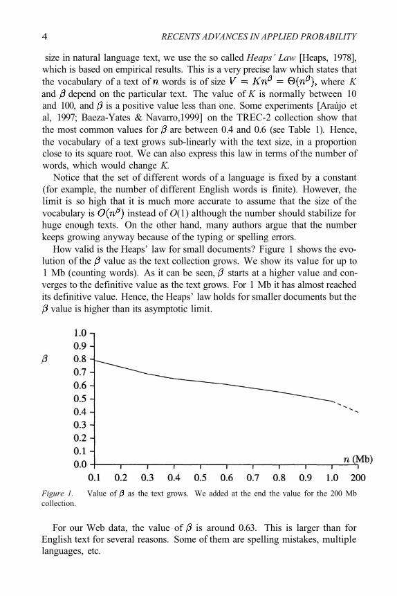
How valid is the Heaps’ law for small documents? Figure 1 shows the evo-lution of the value as the text collection grows. We show its value for up to1 Mb (counting words). As it can be seen, starts at a higher value and con-verges to the definitive value as the text grows. For 1 Mb it has almost reachedits definitive value. Hence, the Heaps’ law holds for smaller documents but the

value is higher than its asymptotic limit.

Figure 1. Value of as the text grows. We added at the end the value for the 200 Mbcollection.

For our Web data, the value of is around 0.63. This is larger than forEnglish text for several reasons. Some of them are spelling mistakes, multiplelanguages, etc.


1.2.3 Distribution of WordsHow are the different words distributed inside each document?. An approx-

imate model is the Zipf’s Law [Zipf, 1949; Gonnet & Baeza-Yates, 1991],which attempts to capture the distribution of the frequencies (that is, numberof occurrences) of the words in the text. The rule states that the frequencyof the most frequent word is times that of the most frequent word.This implies that in a text of words with a vocabulary of V words, themost frequent word appears times, where is the harmonicnumber of order of V, defined as

so that the sum of all frequencies is The value of depends on the text.In the most simple formulation, and thereforeHowever, this simplified version is very inexact, and the case (moreprecisely, between 1.7 and 2.0, see Table 1) fits better the real data [Araújoet al, 1997]. This case is very different, since the distribution is much moreskewed, and Experimental data suggests that a better model is

where c is an additional parameter and is such that all frequenciesadd to This is called a Mandelbrot distribution [Miller, Newman & Fried-man, 1957; Miller, Newman & Friedman, 1958]. This distribution is not usedbecause its asymptotical effect is negligible and it is much harder to deal withmathematically.

It is interesting to observe that if, instead of taking text words, we takeno Zipf-like distribution is observed. Moreover, no good model is

known for this case [Bell, Cleary & Witten, 1990, chapter 4]. On the otherhand, Li [Li, 1992] shows that a text composed of random characters (separa-tors included) also exhibits a Zipf-like distribution with smaller and arguesthat the Zipf distribution appears because the rank is chosen as an indepen-dent variable. Our results relating the Zipf’s and Heaps’ law (see next sec-tion), agree with that argument, which in fact had been mentioned well before[Miller, Newman & Friedman, 1957].

Since the distribution of words is very skewed (that is, there are a few hun-dred words which take up 50% of the text), words that are too frequent, suchas stopwords, can be disregarded. A stopword is a word which does not carrymeaning in natural language and therefore can be ignored (that is, made notsearchable), such as "a", "the", "by", etc. Fortunately the most frequentwords are stopwords, and therefore half of the words appearing in a text donot need to be considered. This allows, for instance, to significantly reduce thespace overhead of indices for natural language texts. Nevertheless, there arevery frequent words that cannot be considered as stopwords.


For our Web data, which is smaller than for English text. Thiswhat we expect if the vocabulary is larger. Also, to capture well the central partof the distribution, we did not take in account very frequent and unfrequentwords when fitting the model. A related problem is the distribution of(strings of exactly characters), which follow a similar distribution [Egghe,2000].

1.2.4 Average Length of Words

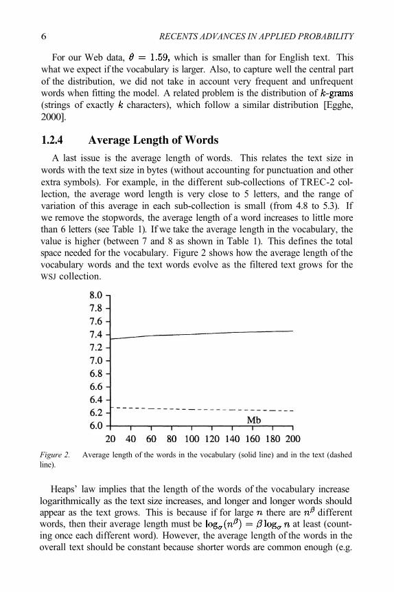
A last issue is the average length of words. This relates the text size inwords with the text size in bytes (without accounting for punctuation and otherextra symbols). For example, in the different sub-collections of TREC-2 col-lection, the average word length is very close to 5 letters, and the range ofvariation of this average in each sub-collection is small (from 4.8 to 5.3). Ifwe remove the stopwords, the average length of a word increases to little morethan 6 letters (see Table 1). If we take the average length in the vocabulary, thevalue is higher (between 7 and 8 as shown in Table 1). This defines the totalspace needed for the vocabulary. Figure 2 shows how the average length of thevocabulary words and the text words evolve as the filtered text grows for theWSJ collection.

Figure 2. Average length of the words in the vocabulary (solid line) and in the text (dashedline).

Heaps’ law implies that the length of the words of the vocabulary increaselogarithmically as the text size increases, and longer and longer words shouldappear as the text grows. This is because if for large there are differentwords, then their average length must be at least (count-ing once each different word). However, the average length of the words in theoverall text should be constant because shorter words are common enough (e.g.


stopwords). Our experiment of Figure 2 shows that the length is almost con-stant, although decreases slowly. This balance between short and long words,such that the average word length remains constant, has been noticed manytimes in different contexts. It can be explained by a simple finite-state modelwhere the separators have a fixed probability of occurrence, since this impliesthat the average word length is one over that probability. Such a model is con-sidered in [Miller, Newman & Friedman, 1957; Miller, Newman & Friedman,1958], where: (a) the space character has probability close to 0.2, (b) the spacecharacter cannot appear twice subsequently, and (c) there are 26 letters.

1.3 Relating the Heaps’ and Zipf’s LawIn this section we relate and explain the two main empirical laws: Heaps’

and Zipf’s. In particular, if both are valid, then a simple relation between theirparameters holds. This result is from [Baeza-Yates & Navarro,1999].

Assume that the least frequent word appears O(1) times in the text (this ismore than reasonable in practice, since a large number of words appear onlyonce). Since there are different words, then the least frequent word hasrank The number of occurrences of this word is, by Zipf’s law,

and this must be O(1). This implies that, as grows, This equal-ity may not hold exactly for real collections. This is because the relation isasymptotical and hence is valid for sufficiently large and because Heaps’and Zipf’s rules are approximations. Considering each collection of TREC-2separately, is between 0.80 and 1.00. Table 1 shows specific values for Kand (Heaps’ law) and (Zipf’s law), without filtering the text. Notice that

is always larger than On the other hand, for our Web data, the match isalmost perfect, as

The relation of the Heapst’ and Zipt’s Laws is mentioned in a line of a paperby Mandelbrot [Mandelbrot, 1954], but no proof is given. In the Appendix

RECENTS ADVANCES IN APPLIED PROBABILITY

we give a non trivial proof based in a simple finite-state model for generatingwords.

1.4 Modeling a Document CollectionThe Heaps’ and Zipf’s laws are also valid for whole collections. In par-

ticular, the vocabulary should grow faster (larger and the word distributioncould be more biased (larger That would match better the relationwhich in TREC-2 is less than 1. However, there are no experiments on largecollections to measure these parameters (for example, in the Web). In addi-tion, as the total text size grows, the predictions of these models become moreaccurate.

1.4.1 Word Distribution Within DocumentsThe next issue is the distribution of words in the documents of a collec-

tion. The simplest assumption is that each word is uniformly distributed inthe text. However, this rule is not always true in practice, since words tend toappear repeated in small areas of the text (locality of reference). A uniformdistribution in the text is a pessimistic assumption since it implies that queriesappear in more documents. However, a uniform distribution can have differentinterpretations. For example, we could say that each word appears the samenumber of times in every document. However, this is not fair if the documentsizes are different. In that case, we should have occurrences proportional tothe document size. A better model is to use a Binomial distribution. That is, if

is the frequency of a word in a set of D documents with words overall, theprobability of finding the word times in a document having words

For large we can use the Poisson approximationwith Some people apply these formulas using the average for allthe documents, which is unfair if document sizes are very different.

A model that approximates better what is seen in real text collections isto consider a negative binomial distribution, which says that the fraction ofdocuments containing a word times is

where and are parameters that depend on the word and the document col-lection. Notice that if we use the averagenumber of words per document, so this distribution also has the problem of be-ing unfair if document sizes are different. For example, for the Brown Corpus

8

is


[Francis & Kucera, 1982] and the word “said”, we have and[Church & Gale, 1995]. The latter reference gives other models derived from aPoisson distribution. Another model related to Poisson which takes in accountlocality of reference is the Clustering Model [Thom & Zobel, 1992].

1.4.2 Distribution of Document SizesStatic databases will have a fixed document size distribution. Moreover, de-

pending on the database format, the distribution can be very simple. However,this is very different for databases that grow fast and in a chaotic manner, suchas the Web. The results that we present next are based in the Web.

The document sizes are self-similar [Crovella & Bestavros, 1996], that is,the probability distribution remains unchanged if we change the size scale. Thesame behavior appears in Web traffic. This can be modeled by two differentdistributions. The main body of the distribution follows a Logarithmic Normalcurve, such that the probability of finding a Web page of bytes is given by

where the average and standard deviation are 9.357 and 1.318, respec-tively [Barford & Crovella, 1998]. See figure of an example in 3 (from [Crov-ella & Bestavros, 1996]).

Figure 3. Left: Distribution for all file sizes. Right: Right tail distribution for different filetypes. All logarithms are in base 10. (Both figures are courtesy of Mark Crovella).

The right tail of the distribution is “heavy-tailed”. That is, the majority ofdocuments are small, but there is a non trivial number of large documents.This is intuitive for image or video files, but it is also true for textual pages. Agood fit is obtained with the Pareto distribution, that says that the probabilityof finding a Web page of bytes is


for and zero otherwise. The cumulative distribution is

where and are constants dependent on the particular collection [Barford& Crovella, 1998]. The parameter is the minimum document size, and isabout 1.36 for textual data, being smaller for images and other binary formats[Crovella & Bestavros, 1996; Willinger & Paxson, 1998] (see the right side ofFigure 3). Taking all Web documents into account, using we get

and 93% of all the files have a size below this value. The parametersof these distributions were obtained from a sample of more than 50 thousandWeb pages requested by several users in a period of two months. Recent resultsshow that these distributions are still valid [Barford et al, 1999], but the exactparameters for the distribution of all textual documents is not known, althoughaverage page size is estimated in 6Kb including markup (which is traditionallynot indexed).

1.5

1.5.1

Models for Queries and Answers

Motivation

When analyzing or simulating text retrieval algorithms, a recurrent problemis how to model the queries. The best solution is to use real users or to extractinformation from query logs. There are a few surveys and analyses of querylogs with respect to the usage of Web search engines [Pollock & Hockley,1997; Jensen et al, 1998; Silverstein et al, 1998]. The later reference is thestudy of 285 million AltaVista user sessions containing 575 million queries.Table 2 gives some results from that study, done in September of 1998. Anotherrecent study on Excite, shows similar statistics, and also the queries topics[Spink et al, 2002]. Nevertheless, these studies give little information aboutthe exact distribution of the queries. In the following we give simple modelsto select a random query and the corresponding average number of answersthat will be retrieved. We consider exact queries and approximate queries. Anapproximate query finds a word allowing up to errors, where we count theminimal number of insertions, deletions, and substitutions.

1.5.2 Random QueriesAs half of the text words are stopwords, and they are not typical user queries,

stopwords are not considered. The simplest assumption is that user queriesare distributed uniformly in the vocabulary, i.e. every word in the vocabularycan be searched with the same probability. This is not true in practice, sinceunfrequent words are searched with higher probability. On the other hand,


approximate searching makes this distribution more uniform, since unfrequentwords may match with errors with other words, with little relation to thefrequencies of the matched words. In general, however, the assumption ofuniform distribution in the vocabulary is pessimistic, at least because a matchis always found.

Looking at the results in the AltaVista log analysis [Silverstein et al, 1998],there are some queries much more popular than others and the range is quitelarge. Hence, a better model would be to consider that the queries also followa Zipf’s like distribution, perhaps with larger than 2 (the log data is not avail-able to fit the best value). However, the actual frequency order of the wordsin the queries is completely different from the words in the text (for example,“sex” and “xxx” appear between the top most frequent word queries), whichmakes a formal analysis very difficult. An open problem, which is related tothe models of term distribution in documents, is whether the distribution forquery terms appearing in a collection of documents is similar to that of docu-ment terms. This is very important as these two distributions are the base forrelevance ranking in the vector model [Baeza-Yates & Ribeiro-Neto, 1999].Recent results show that although queries also follow a Zipf distribution (withparameter from 1.24 to 1.42 [Baeza-Yates & Castillo, 2001; Baeza-Yates &Saint-Jean, 2002]), the correlation to the word distribution of the text is low(0.2) [Baeza-Yates & Saint-Jean, 2002]. This implies that choosing queries atrandom from the vocabulary is reasonable and even pessimistic.

Previous work by DeFazio [DeFazio, 1993] divided the query vocabulary inthree segments: high (words representing the most used 90% of the queries),moderate (next 5% of the queries), and low use (words representing the leastused 5% of the queries). Words are then generated by first randomly choosingthe segment, the randomly picking a token within that segment. Queries areformed by choosing randomly one to 50 words. According to currently avail-able data, real queries are much shorter, and the generation algorithm does notproduce the original query distribution. Another problem is that the query vo-cabulary must be known to use this model. However, in our model, we cangenerate queries from the text collection.


1.5.3 Number of Answers

Now we analyze the expected number of answers that will be obtained us-ing the simple model of the previous section. For a simple word search, wewill find just one entry in the vocabulary matching it. Using Heaps’ law, theaverage number of occurrences of each word in the text isHence, the average number of occurrences of the query in the text isThis fact is surprising, since one can think in the process of traversing the textword by word, where each word of the vocabulary has a fixed probability ofbeing the next text word. Under this model the number of matching wordsis a fixed proportion of the text size (this is equivalent to say that a word oflength should appear about times). The fact that this is not the case(demonstrated experimentally later) shows that this model does not really holdon natural language text.

The root of this fact is not in that a given word does not appear with afixed probability. Indeed, the Heaps’ law is compatible with a model whereeach word appears at fixed text intervals. For instance, imagine that Zipf’slaw stated that the word appeared times. Then, the first word couldappear in all the odd positions, the second word in all the positions multipleof 4 plus 2, the third word in all the multiples of 8 plus 4, and so on. Thereal reason for the sublinearity is that, as the text grows, there are more words,and one selects randomly among them. Asymptotically, this means that thelength of the vocabulary words must be and therefore, as thetext grows, we search on average longer and longer words. This allows thateven in the model where there are matches, this number is indeed[Navarro, 1998]. Note that this means that users search for longer words whenthey query larger text collections, which seems awkward but may be true, asthe queries are related to the vocabulary of the collection.

How many words of the vocabulary will match an approximate query? Inprinciple, there is a constant bound to the number of distinct words whichmatch a given query with errors, and therefore we can say that O(1) wordsin the vocabulary match the query. However, not all those words will appearin the vocabulary. Instead, while the vocabulary size increases, the numberof matching words that appear increases too, at a lower rate. This is the samephenomenon observed in the size of the vocabulary. In theory, the total numberof words is finite and therefore V = O(1), but in practice that limit is neverreached and the model describes reality much better. We showexperimentally that a good model for the number of matching words in thevocabulary is (with Hence, the average number of occurrencesof the query in the text is [Baeza-Yates & Navarro, 1999].


1.5.4 ExperimentsWe present in this section empirical evidence supporting our previous state-

ments. We first measure V, the number of words in the vocabulary in terms of(the text size). Figure 4 (left side) shows the growth of the vocabulary. Using

least squares we fit the curve The relative error is very small(0.84%). Therefore, for the WSJ collection.

We measure now the number of words that match a given pattern in thevocabulary. For each text size, we select words at random from the vocabularyallowing repetitions. In fact, not all user queries are found in the vocabulary in

Figure 4. Vocabulary tests for the WSJ collection. On the left, the number of words in thevocabulary. On the right, number of matching words in the vocabulary.


practice, which reduces the number of matches. Hence, this test is pessimisticin that sense.

We test and 3 errors. To avoid taking into account queries withvery low precision (e.g. searching a 3-letter word with 2 errors may match toomany words), we impose limits on the length of words selected: only words oflength 4 or more are searched with one error, length 6 or more with two errors,and 8 or more with three errors.

We perform a number of queries which is large enough to ensure a relativeerror smaller than 5% with a 95% confidence interval. Figure 4 (right side)shows the results. We use least squares to fit the curves for

for and for In all cases the relative errorof the approximation is under 4%. The exponents are the values mentionedlater in this article. One possible model for is because for

we have and when as expected.We could reduce the variance in the experiments by selecting once the set

of queries from the index of the first 20 Mb. However, our experiments haveshown that this is not a good policy. The reason is that the first 20 Mb willcontain almost all common words, whose occurrence lists grow faster than theaverage. Most uncommon words will not be included. Therefore, the resultwould be unfair, making the results to look linear when they are in fact sublin-ear.

1.6 Application: Inverted Files for the Web

1.6.1 Motivation

Web search engines currently available use inverted files that reference Webpages [Baeza-Yates & Ribeiro-Neto, 1999]. So, reference pointers should haveas many bits as needed to reference all Web pages (currently, about 3 billion).The number and size of pointers is directly related with the space overhead ofthe inverted file. For the whole Web, this implies at least 600 GB. Some searchengines also index word locations, so the space needed is increased. One wayto reduce the size of the index is to use fixed logical blocks as reference units,trading the reduction of space obtained with an extra cost at search time. Theblock mechanism is a logical layer and the files do not need to be physicallysplit or concatenated. In which follows we explain this technique in moredetail.

Assume that the text is logically divided into “blocks”. The index stores allthe different words of the text (the vocabulary). For each word, the list of theblocks where the word appears is kept. We call the size of the blocks and

the number of blocks, so that The exact organization is shown inFigure 5. This idea was first used in Glimpse [Manber & Sun Wu, 1994].


Figure 5. The block-addressing indexing scheme.

At this point the reader may wonder which is the advantage of pointing toartificial blocks instead of pointing to documents (or files), this way followingthe natural divisions of the text collection. If we consider the case of simplequeries (say, one word), where we are required to return only the list of match-ing documents, then pointing to documents is a very adequate choice. More-over, as we see later, it may reduce space requirements with respect to usingblocks of the same size. Moreover, if we pack many short documents in a log-ical block, we will have to traverse the matching blocks (even for these simplequeries) to determine which documents inside the block actually matched.

However, consider the case where we are required to deliver the exact posi-tions which match a pattern. In this case we need to sequentially traverse thematching blocks or documents to find the exact positions. Moreover, in sometypes of queries such as phrases or proximity queries, the index can only tellthat two words are in the same block, and we need to traverse it in order todetermine if they form a phrase.

In this case, pointing to documents of different sizes is not a good ideabecause larger documents are searched with higher probability and searchingthem costs more. In fact, the expected cost of the search is directly relatedto the variance in the size of the pointed documents. This suggests that if thedocuments have different sizes it may be a good idea to (logically) partition


large documents into blocks and to put together small documents, such thatblocks of the same size are used.

In [Baeza-Yates & Navarro,1999], we show analytically and experimentallythat using fixed size blocks it is possible to have a sublinear-size index withsublinear search times, even for approximate word queries. A practical exam-ple shows that the index can be in space and in retrieval time for ap-proximate queries with at most two errors. For exact queries the exponent low-ers to 0.85. This is a very important analytical result which is experimentallyvalidated and makes a very good case for the practical use of this kind of in-dex. Moreover, these indices are amenable to compression. Block-addressingindices can be reduced to 10% of their original size [Bell et al, 1993], and thefirst works on searching the text blocks directly in their compressed form arejust appearing [Moura et al, 1998a; Moura et al, 1998] with very good perfor-mance in time and space.

Resorting to sequential searching to solve a query may seem unrealistic forcurrent Web search engine architectures, but makes perfect sense in a near fu-ture when a remote access could be as fast as a local access. Another practicalscenario is a distributed architecture where each logical block is a part of a Webserver or a small set of Web servers locally connected, sharing a local index.

As explained before, pointing to documents instead of blocks may or maynot be convenient in terms of query times. We analyze now the space and laterthe time requirements when we point to Web pages or to logical blocks of fixedsize. Recall that the distribution has a main body which is log-normal (that weapproximate with a uniform distribution) and a Pareto tail.

We start by relating the free parameters of the distribution. We call C the cutpoint between both distributions and the fraction of documents smaller thanC. Since Then the integral over the tail (from C to infinity) must bewhich implies that We also need to know the value of thedistribution in the uniform part, which we call and it holds Forthe occurrences of a word inside a document we use the uniform distributiontaking into account the size of the document.

1.6.2 Space Overhead

As the Heaps’ law states that a document with words has differentwords, we have that each new document of size added to the collection willinsert new references to the lists of occurrences (since each different wordof each different document has an entry in the index). Hence, an index ofblocks of size takes space. If, on the other hand, we consider the Webdocument size distribution, we have that the average number of new entries in


the occurrence list per document is

where was defined in Section 1.4.2.To determine the total size of the collection, we consider that documents

exist, whose average length is given by

and therefore the total size of the collection is

The final size of the occurrence lists is (using Eq. (6.1))

We consider now what happens if we take the average document lengthand use blocks of that fixed size (splitting long documents and putting shortdocuments together as explained). In this case, the size of the vocabulary is

as before, and we assume that each block is of a fixed size Wehave introduced a constant to control the size of our blocks. In particular, ifwe use the same number of blocks as Web pages, then Then the size ofthe lists of occurrences is

(using Eq. (6.3)). Now, if we divide the space taken by the index of documentsby the space taken by the index of blocks (using the previous equation andEq. (6.4)), the ratio is


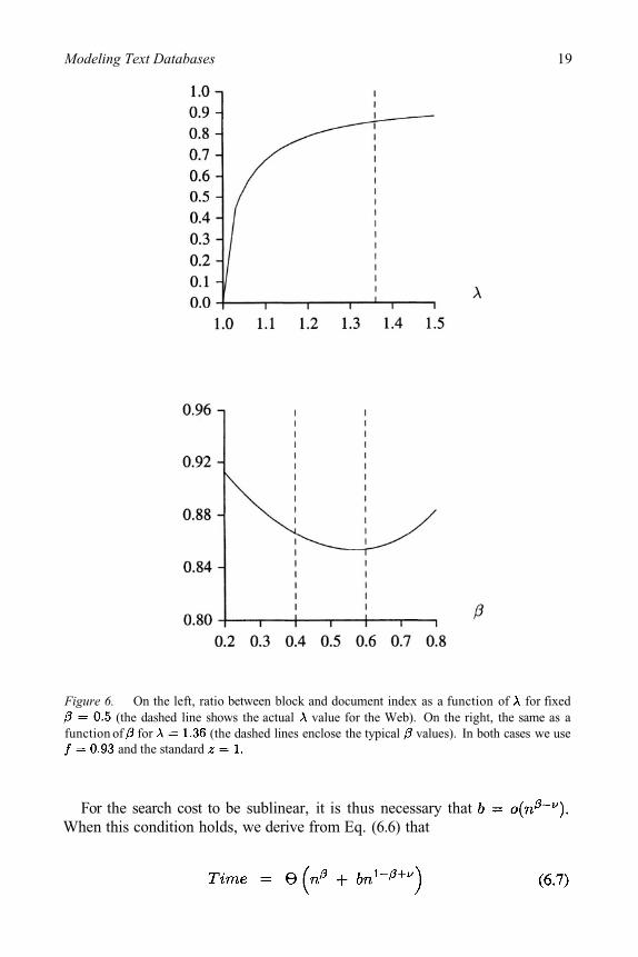
which is independent of and C; and is about 85% forand We approximated which corresponds to all theWeb pages, because the value for textual pages is not known. This shows thatindexing documents yields an index which takes 85% of the space of a blockaddressing index, if we have as many blocks as documents. Figure 6 shows theratio as a function of and As it can be seen, the result varies slowly with

while it depends more on (tending to 1 as the document size distributionis more uniform).

The fact that the ratio varies so slowly with is good because we alreadyknow that the value is quite different for small documents. As a curiosity, seethat if the documents sizes were uniformly distributed in all the range (that is,letting the ratio would become which is close to 0.94 forintermediate values. On the other hand, letting (as in the simplifiedmodel [Crovella & Bestavros, 1996]) we have a ratio near 0.83. As anothercuriosity, notice that there is a value which gives the minimum ratio fordocument versus block index (that is, the worst behavior for the block index).This is for quite close to the real values (0.63 in our Webexperiments).

If we want to have the same space overhead for the document and the blockindices, we simply make the expression of Eq. (6.5) equal to 1 and obtain

for that is, we need to make the blocks largerthan the average of the Web pages. This translates into worse search times. Bypaying more at search time we can obtain smaller indices (letting grow over1.48).

1.6.3 Retrieval Time

We analyze the case of approximate queries, given that for exact queriesthe result is the same by using The probability of a given word to beselected by a query is The probability that none of the words in ablock is selected is therefore The total amount of work of anindex of fixed blocks is obtained by multiplying the number of blocks timesthe work to do per selected block times the probability that some word inthe block is selected. This is

where for the last step we used thatprovided

We are interested in determining in which cases the above formula is sub-linear in Expressions of the form are whenever(since On the other hand, if then is faraway from 1, and therefore is


Figure 6. On the left, ratio between block and document index as a function of for fixed(the dashed line shows the actual value for the Web). On the right, the same as a

function of for (the dashed lines enclose the typical values). In both cases we useand the standard

For the search cost to be sublinear, it is thus necessary thatWhen this condition holds, we derive from Eq. (6.6) that


We consider now the case of an index that references Web pages. As wehave shown, if a block has size then the probability that it has to be traversedis We multiply this by the cost to traverse it and integrateover all the possible sizes, so as to obtain its expected traversal cost (recallEq. (6.6))

which we cannot solve. However, we can separate the integral in two parts, (a)and (b) In the first case the traversal probability

is and in the second case it is Splitting the integral in twoparts and multiplying the result by we obtain the total amount ofwork:

where since this is an asymptotic analysis we have consideredas C is constant.

On the other hand, if we used blocks of fixed size, the time complexity(using Eq. (6.7)) would be where The ratio betweenboth search times is

which shows that the document index would be asymptotically slower thana block index as the text collection grows. In practice, the ratio is between

and . The value of is not important here since it is a constant,but notice that is usually quite large, which favors the block index.

1.7 Concluding Remarks

The models presented here are common to other processes related to humanbehavior [Zipf, 1949] and algorithms. For example, a Zipf like distributionalso appears for the popularity of Web pages with [Barford et al, 1999].On the other hand, the phenomenon of sublinear vocabulary growing is not ex-clusive of natural language words. It appears as well in many other scenarios,such as the number of different words in the vocabulary that match a givenquery allowing errors as shown in Section 5, the number of states of the de-terministic automaton that recognizes a string allowing errors [Navarro, 1998],and the number of suffix tree nodes traversed to solve an approximate query[Navarro & Baeza-Yates, 1999]. We believe that in fact the finite state modelfor generating words used in Section 3 could be changed for a more general