receiving antenna alignment in hexagonal grid simulations: a … · receiving antenna alignment...

Receiving Antenna Alignment

in Hexagonal Grid Simulations:

A Study for LTE-based 5G

Terrestrial Broadcast

FEBRUARY 2020

Simon Elliott, BBC

Jordi Joan Gimenez, IRT

Assunta De Vita, RAI

David Vargas, BBC

EBU Technology & Innovation | Technical Review | JAN 2020 2

The main purpose of an EBU Technical Review is to critically examine new

technologies or developments in media production or distribution. All Technical

Reviews are reviewed by 1 (or more) technical experts at the EBU or externally and

by the EBU Technical Editions Manager. Responsibility for the views expressed in

this article rests solely with the author(s).

To access the full collection of our Technical Reviews, please see:

tech.ebu.ch/publications

If you are interested in submitting a topic for an EBU Technical Review, please

contact: [email protected] .

mailto:[email protected]


1. Introduction

Over the last few years EBU members have been collaborating with the mobile

industry in order to make the enhanced Multicast Broadcast Multimedia Service

(eMBMS), defined in the Third Generation Private Partnership (3GPP) mobile

communication system standards, more suitable for delivering broadcasters’ content.

The collaboration has so far been very fruitful, with eMBMS being further evolved in

the Enhanced TV (enTV) Work Item of Long-Term Evolution (LTE) Release 14

(Rel-14) specifications.

Rel-16 has further enhanced eMBMS with greater support for conventional

broadcasting in the LTE-based 5G Terrestrial Broadcast1 [1, 2] work item. A longer

Cyclic Prefix (CP) has been added to support single frequency networks (SFN) with

inter-site distances (ISD) more typically found in high power high tower (HPHT)

broadcast networks. In addition, a shorter CP for greater mobility up to 250 km/h has

been introduced, and the cell acquisition subframe (CAS) has been made more

robust. EBU members continue to contribute to 3GPP.

3GPP makes extensive use of Monte Carlo based network simulations in order to

evaluate the benefits of any potential enhancements before they are standardised.

The enTV Work Item permitted the simulations to use several different methodologies

for the alignment of directional receiving antennas to transmitter sites and for

determining which signals are permitted to contribute to the useful signal.

This article investigates several different methodologies that are commonly used in

these two aspects of the simulations and, using 5G broadcast as an example,

illustrates how the different methodologies affect the results. Detailed worked

examples are also provided for clarity.

2. 5G Broadcast: Background

LTE Rel-14 is the first 3GPP specification targeting the delivery of TV services in a

similar way to conventional terrestrial broadcast standards [3]. For example, Rel-14

introduces carriers with 100% downlink capacity for broadcast services for which

SIM-free reception without uplink is possible, and additional OFDM parameters

(numerologies) for the support of fixed rooftop reception in SFN with an ISD of 15 km

or more in low power low tower (LPLT) networks.

An extensive analysis of the broadcast related features introduced in Rel-14 can be

found in [4] and [5]. A Rel-16 study [1] identified gaps between LTE Rel-14 eMBMS

and the 5G requirements for dedicated broadcast networks in [3]. Rel-16 added

further enhancements to make 5G Broadcast suitable for deployments in large area

SFN with ISDs of around 100 km or more, increase mobility up to 250 km/h, and

make the systems signal acquisition and synchronisation mechanisms more robust.

1 LTE-based 5G Terrestrial Broadcast is here referred to as 5G Broadcast


2.1 Numerologies for SFN Deployments

LTE Rel-14 introduced two new numerologies for the MBSFN (multicast-broadcast

single frequency network) radio bearer of eMBMS. The sub-carrier spacings of the

new numerologies are 7.5 kHz and 1.25 kHz, with CP durations of 33.3 µs and

200 µs, respectively.

LTE Rel-16 introduced an additional two numerologies with sub-carrier spacings of

2.5 kHz and 0.37 kHz, with CP durations of 100 µs and 300 µs, respectively [2]. The

wider carrier spacing of the 2.5 kHz numerology supports greater mobility up to

250 km/h. The 300 µs CP numerology is designed to support fixed rooftop reception

in SFN with large ISDs typically found in HPHT broadcast networks.

Table 1 sets out the sub-carrier spacing (𝛥𝑓), CP duration (TCP), useful symbol period

(TU) and equalisation interval2 (EI) for the numerologies in 5G Broadcast. The longest

CP permitted in Rel-14 was 200 µs (OFDM symbol duration TS = TU + TCP = 1 ms).

Rel-16 includes a 300 µs CP with an OFDM symbol duration of 3 ms.

While the MBSFN subframes (containing data) can only be configured with large

“Extended CP” configurations, the cell acquisition subframe (CAS), containing control

and synchronisation information, are restricted to the “Normal” and “Extended” CP

configurations with a sub-carrier spacing of 15 kHz.

The 1 ms CAS, configured with normal CP, has 14 OFDM symbols and the CAS

configured with extended CP has 12 OFDM symbols. For the rest of the paper we

assume the extended CP configuration for the CAS due to its ability to tolerate

echoes with longer delays.

Table 1: Rel-14/16 eMBMS Numerologies

𝜟𝒇 (kHz) TCP (µs) TU (µs) CAS EI (µs) EI (µs)

Normal CP 15 4.7/5.2 66.7 - -

Extended CP

(Rel-14)

15 16.7 66.7 22.2 66.7

7.5 33.3 133.3 - 66.7

1.25 200 800 - 267

Extended CP (added in Rel-16)

2.5 100 400 - 200

0.37 300 2,700 - 900

2 The equalisation interval (EI) is the Nyquist limit of the receivers channel equalisation filter. The EI denotes the maximum echo delay for which a receiver may correctly equalise a transmitted signal. It is dependent on the effective frequency separation of the reference signal (RS) [6].


2.2 Framing and Cell Acquisition Subframe (CAS)

The introduction of a 100% broadcast mode required changes to the conventional

frame structure of LTE. The new 100% broadcast radio frame is 40 ms in duration

(Figure 1). It is made up of the new CAS with a duration of 1 ms followed by

39 MBSFN subframes each with a duration of 1ms for numerologies with 7.5 kHz,

2.5 kHz and 1.25 kHz sub-carrier spacings. With the 0.37 kHz sub-carrier

numerology (300 µs CP), the frame structure consists of one CAS subframe with a

duration of 1 ms followed by 13 MBSFN subframes, each with a duration of 3 ms.

Figure 1: 100% Broadcast Radio Frame.

The CAS contains the essential signalling for demodulating the user plane data [5].

The physical channels comprising the CAS are shown in Figure 2.

Figure 2: Channels comprising the CAS

The CAS uses CS-RS (Cell Specific Reference Signals) that are inherited from the

unicast design, meaning that the CAS can only achieve a maximum 22 µs EI, as

shown in Table 1. A numerology mismatch between the CAS and the MBSFN

subframes therefore arises as the MBSFN subframes can be configured with CPs of

33.3 µs, 100 µs, 200 µs and 300 µs, while the maximum CP duration for the CAS is

16.7 µs.

The CAS must be correctly decoded before the PMCH (Physical Multicast Channel),

which conveys the MBSFN subframes, can be received. It is therefore essential that

the CAS is designed to be sufficiently robust so as to ensure adequate reception of

the PMCH in locations where the CAS is not protected by the longer CP of the

MBSFN subframes.


Rel-16 made the CAS more robust by different methods, including greater repetition

of the information in the sub-channels, to increase detection probability. The changes

do not include modifications in the numerologies as this would have needed a

re-design of the control channels already defined for LTE.

3. Network Simulation Background

A framework for performing Monte Carlo based network simulations for 5G Broadcast

in Rel-16 is set out in [1]. It describes the network topology, such as the locations of

transmitter sites, their effective heights and radiated powers, the propagation model,

the receiver’s noise floor, receiving antenna patterns, etc.

The simulation network comprises 61 transmitters configured as shown in Figure 3.

Figure 3: Hexagonal Network Layout and Coverage Area for the MPMT Network.

All 61 transmitters are allocated the same frequency and belong to a single MBSFN

area. Multiple frequency networks (MFN) are outside the scope of the framework.

Other key simulation parameters are shown in Table 2.


Table 2: Main Simulation Parameters

Parameter Value

Inter-site Distance 50 km

Transmitter Effective Height 100 m

Transmitting Antenna Omni-directional

Effective Radiated Power (E.R.P.) 40.5 dBW EIRP

Receiving Antenna Height 10 m

Receiver Noise Figure 6 dB

Rx Antenna Pattern ITU-R BT.419/Omni-Directional

Rx Antenna Gain (Omni/Directional) 0 / 13.15 dBi

Antenna Cable Loss 4 dB

Implementation Margin 1 dB

Noise Bandwidth 9 MHz

Frequency 700 MHz

Propagation Model ITU-R P.1546-5 over land

Wanted Signal Time Value 50%

Interfering Signal Time Value 1%

Location Variation (µ/σ) 0 dB/5.5 dB (log-normal distribution)

Simulation Methodology Monte Carlo

Pixel Size 100 m x 100 m

Tx/Rx Error Vector Magnitude (EVM)3 8% / 4%

Handover Margin None

SFN Signal Summation SFN weighting function [6]

Measurements show that, due to variations in terrain and ground cover, the signals

from transmitters will vary from one location to another throughout a small area e.g. a

square ‘pixel’ with sides of 100 m. This location variation is modelled by a log-normal

distribution with a mean of 0 dB and standard deviation of 5.5 dB. Location variation

is a crucial concept in this document – it plays a key role in the network simulations.

All the simulations in this study have been carried out within a single square pixel of

side 100 m, centred at the apex of the central ‘red hexagon’ marked by the green dot

in Figure 3. Within this pixel, 10000 realisations of location variation were generated

for each transmitter. The SINR was then computed from these realisations using the

receiving antenna alignment methodologies described below.

The selected pixel is representative of the coverage area with interference from

multiple distant transmitters and although coverage will vary over the entire network,

restricting the analysis to a single representative pixel is a convenient way to

3 In this document the EVM of the transmitter and the receiver has been set to 0% i.e. both are ideal.


compare the effects of different simulation methodologies. The examples in the

Annex provide more detail on the SINR calculations within such a pixel.

3.1 Receiving Antenna Alignment for Roof-top Reception

Three methodologies have been considered when determining how to align

directional receiving antennas (no alignment is necessary for omni-directional

antennas):

- Wanted Transmitter: the main lobe of the receiving antenna is aligned to a

specific transmitter, defined as the wanted transmitter, before the simulation

begins. This option is commonly used for pixel-based simulations.

- Closest Transmitter: the main lobe of the receiving antenna is aligned to the

closest transmitter. Due to the regular nature of the transmitter networks used

herein, and the monotonic decay of the ITU-R P.1546-5 field strength with

distance, this alignment is equivalent to aligning the receiving antenna with the

transmitter that provides the strongest field strength before location variation is

applied.

- Strongest Transmitter: the main lobe of the receiving antenna is aligned to the

transmitter that provides the strongest field strength at the receiving location, after

location variation has been applied.

3.2 Contributing Signals in SFN and ASFN Network Configurations

Several different options may be used to determine which signals may contribute

constructively to the wanted signal. The options depend on the network configuration.

Two different networks have been considered in this document: conventional SFN

and Asynchronous SFN (ASFN), as described below.

• SFN: a conventional SFN in which the content from all transmitters is

synchronised in both time and frequency so that signals from multiple transmitters

may contribute to the wanted signal, the extent of which is determined with the

well-known SFN weighting function [6].

- All Transmitters Contribute to the Wanted: in the case of SFN, all

transmitters may contribute to the wanted signal. In the examples herein

there is only one MBSFN area, so all 61 transmitters may contribute to the

wanted signal.

• ASFN: all transmitters transmit on the same frequency as in a conventional SFN,

but their content is not synchronised. In these networks the signals from each

transmitter would interfere with one another, regardless of the CP duration and

the signals’ relative delays. At each receiving location it is therefore necessary to

define a single transmitter that provides the wanted signal within ASFN. Three

options have been considered:


- Wanted: at all receiving locations, only the wanted transmitter, defined

before the simulation begins, is permitted to provide the wanted signal. All

other transmitters are defined as interferers.

- Closest: at each receiving location, only the closest transmitter may

provide the wanted signal. All other transmitters are defined as interferers.

- Strongest Transmitter: only the signal from the transmitter providing the

strongest field strength at the receiving location, after the application of

location variation and the receiving antenna pattern (based on the

alignment strategy above), contributes to the wanted signal. All other

transmitters are defined as interferers.

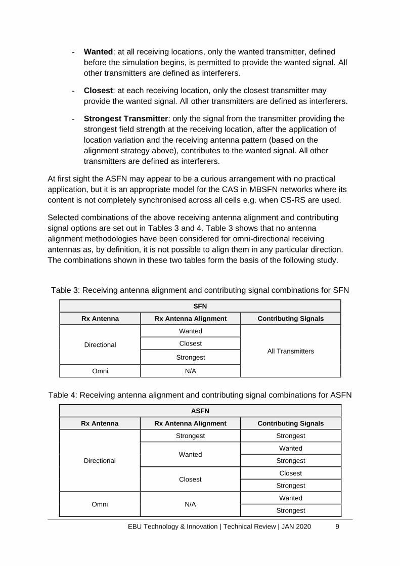
At first sight the ASFN may appear to be a curious arrangement with no practical

application, but it is an appropriate model for the CAS in MBSFN networks where its

content is not completely synchronised across all cells e.g. when CS-RS are used.

Selected combinations of the above receiving antenna alignment and contributing

signal options are set out in Tables 3 and 4. Table 3 shows that no antenna

alignment methodologies have been considered for omni-directional receiving

antennas as, by definition, it is not possible to align them in any particular direction.

The combinations shown in these two tables form the basis of the following study.

Table 3: Receiving antenna alignment and contributing signal combinations for SFN

SFN

Rx Antenna Rx Antenna Alignment Contributing Signals

Directional

Wanted

All Transmitters Closest

Strongest

Omni N/A

Table 4: Receiving antenna alignment and contributing signal combinations for ASFN

ASFN

Rx Antenna Rx Antenna Alignment Contributing Signals

Directional

Strongest Strongest

Wanted Wanted

Strongest

Closest Closest

Strongest

Omni N/A Wanted

Strongest


4. Simulation Results

4.1 Single Frequency Networks (SFN) with Directional Receiving Antennas

This section presents and discusses the results for SFN in which all transmitters may

contribute to the wanted signal. Figure 4 shows the complementary CDF of the SINR

achieved at the apex of the central hexagon for the receiving antenna alignment

options in Table 3 and two different CP durations. The 300 µs numerology achieves a

higher SINR than the 200 µs numerology as the longer CP reduces SFN

self-interference.

Figure 4: Achievable SINR for different directional receiving

antenna alignment strategies in SFN

Due to the symmetry of the network and the location of the pixel that is being

considered, aligning the receiving antenna to the wanted and closest transmitters at

each location achieves identical SINRs.

Aligning the receiving antenna to the strongest transmitter at each location produces

a markedly higher SINR than the other two methods for both CPs. With this method,

at every receiving location the receiving antenna is aligned to the strongest signal

after location variation has been applied. The wanted signal level is thus maximised,

as well as the SINR.

It is worthwhile noting that the shape of the curves may change from one receiving

location to another; at some locations there will be a greater or lesser effect of one

antenna alignment method over the other. Nevertheless, the principle remains that


different methodologies may significantly affect the coverage results. It is therefore

important to know, and to clearly state, which methodologies were used when results

are presented.

4.2 Asynchronous Single Frequency Networks (ASFN)

In ASFN networks it is necessary to define at each location which transmitter

provides the wanted signal. It should be expected that defining the wanted

transmitter in different ways will affect the simulation result. The combinations of

receiving antenna alignment and permitted contributing signals set out in § 3.2 are

investigated below.

4.2.1 Directional Receiving Antenna

Figure 5 shows the results for the directional receiving antenna simulations.

Figure 5: Achievable SINR with a directional receiving antenna in an ASFN

In this example, due to the symmetry of the network, the SINR curves are identical

for the receiving antenna aligned to the closest transmitter, receive the signal from

the closest transmitter methodology and receiving antenna aligned to the wanted

transmitter, receive the signal from the wanted transmitter.

Similarly, the curves are identical for the receiving antenna aligned to the closest

transmitter, receive strongest signal methodology and receiving antenna aligned to

wanted transmitter, receive strongest signal methodology. However, at high coverage

probabilities (e.g. >95% locations), defining the wanted signal as the strongest signal

(after location variation and receiving antenna alignment) marginally improves the


SINR compared with restricting the wanted signal to the one originating from the

transmitter to which the receiving antenna has been aligned.

A significantly higher SINR is achieved by aligning the receiving antenna to the

strongest signal at each receiving location (after the application of location variation),

and to defining the strongest signal as the Wanted.

4.2.2 Omni-Directional Receiving Antenna

This section investigates reception of an ASFN with an omni-directional receiving

antenna – a network configuration suitable for modelling the CAS, which may not be

fully synchronised, for reception with mobile devices (assumed to have omni-

directional antennas). The results for the Wanted and Strongest transmitter methods

are shown in Figure 6.

Defining the strongest signal as the wanted signal, as opposed to only permitting the

wanted signal to come from a pre-defined wanted transmitter, significantly improves

the achievable SINR. In this example the difference between the two methodologies

for the 95th percentile is approximately 13 dB.

Allowing the mobile device to receive the strongest signal at each location in the

model is appropriate as these devices have no receiving antenna pattern to align to

any particular transmitter. This model is therefore considered to be more appropriate

for mobile reception than restricting the device to consider a pre-defined signal as the

wanted signal, particularly in the cases where there is no requirement to deliver

regional content at border regions.

Figure 6: Achievable SINR with an omni-directional receiving antenna in an ASFN


5. Conclusions

This article has outlined several different methodologies that are commonly used in

network simulations in order to align receiving antennas and to define the

transmitters which may contribute to the wanted signal.

It is clear from the network simulation results that different methodologies may

significantly affect their outcome. It is therefore important to clearly state the

methodology that has been used when presenting such results so that they can be

correctly interpreted.

With respect to 5G Broadcast, a critical topic has been to understand how robust the

CAS would need to be in order to ensure that this essential signal is adequately

received.

As shown in this article, different methodologies for determining which transmitters

may contribute to the wanted signal in a mobile receiving environment can make a

significant difference to the achievable SINR in the network (circa 13 dB).

When evaluating the performance of signals, such as the CAS, it is important to apply

simulation methodologies that reflect the receiving environment so that the

transmission standard may be appropriately designed. Over-designing the system

may be too costly, while under-designing the system may lead to a poor user

experience.


Annex: Antenna Alignment Examples

Three very simple examples are now presented in order to illustrate how different

receiving antenna alignment algorithms may affect the results of otherwise identical

simulations. The examples are based on the trivial three transmitter network shown in

Figure 7 configured as an ASFN. Each transmitter is located at the centre of three

regular hexagons whose apexes meet at the geographic centre of the network. For

simplicity we focus on a square pixel of side 100 m located at this central point, but

as the concepts involved here are general in nature, any other location could have

been chosen.

All three transmitters have the same effective height, effective radiated power (ERP)

and omni-directional antenna pattern. Due to the symmetry of the network, and the

ITU-R P.1546 propagation model, which decays monotonically with distance, each

transmitter generates the same median signal strength in the central pixel for any

specific percentage of the time. In the examples below the median field strength

generated by each transmitter in the pixel is taken to be 70 dB µV/m for 50% of the

time. The 1%-time levels are 72 dB µV/m.

The convention of computing wanted and interfering signals at their 50%-time and

1%-time levels, respectively, has also been used. Thermal noise has been excluded

for simplicity.

Figure 7: Three transmitter network and central pixel

Within the pixel the field strength from each transmitter will naturally vary from one

receiving location to another due to location variation (e.g. signal blockage due to

buildings, vegetation, etc.). Assuming there is no correlation in the signal levels

generated by any of the transmitters at any location within the pixel, the field strength

of each transmitter can be calculated at each location:

𝐹𝑖𝑗 = �̃�𝑖 + 𝐿𝑖𝑗 (1)

Where 𝐹𝑖𝑗 is the field strength from transmitter 𝑖 generated at location 𝑗 within a pixel.

�̃�𝑖 is the median field strength within the pixel generated by transmitter 𝑖. 𝐿𝑖𝑗 is the

value of the location dependant variation for transmitter 𝑖 at location 𝑗. The location


variation is approximated by a log-normal distribution of mean (µ) 0 dB and standard

deviation (σ) 5.5 dB.

Table 5 shows an example of the 50%-time field strengths from each of the three

transmitters that could be found at three arbitrary locations inside the central pixel,

and how they were derived from a median signal level. The location variation value

(𝐿) has been randomly drawn from the log-normal distribution previously described.

The 1% time-values are 2dB higher.

Table 5: Field strengths in the central pixel, for the 50%-time levels.

Location 1 Location 2 Location 3

�̃� (dBµV/m)

𝑳 (dB)

𝑭 (dBµV/m)

�̃� (dBµV/m)

𝑳 (dB)

𝑭 (dBµV/m)

�̃�

(dBµV/m)

𝑳 (dB)

𝑭 (dBµV/m)

Tx 1 70 7 77 70 -9 61 70 -8 62

Tx 2 70 3 73 70 11 81 70 5 75

Tx 3 70 -5 65 70 -3 67 70 7 77

Figure 8 illustrates the situation within the pixel where the 50%-time signal levels

have plain type and the 1%-time values are italicised.

Figure 8: Field strengths in the central pixel

A1 Rx Antenna aligned with Wanted Tx; Only the Wanted Tx is Permitted

to Provide Wanted Signal

In this example Tx 1 is defined as the wanted transmitter. The directional receiving

antenna is then aligned to this transmitter, and only this transmitter may provide the

wanted signal. Once these definitions have been made, the appropriate wanted

(50%-time) and interfering (1%-time) field strengths (𝐹𝑖𝑗) at each location become

those shown in Figure 9a. The receiving antenna, with the pattern in Figure 9b is

aligned to Tx 1 at all receiving locations within the pixel. The effective field strengths

(𝐹𝑒 𝑖𝑗) that would be received from each transmitter at each location after the

receiving antenna pattern has been applied are then shown in Figure 9c.


𝐹𝑒 𝑖𝑗 is simply the sum of the appropriate field strength from each transmitter at each

location (𝐹𝑖𝑗) and the appropriate attenuation of the receiving antenna pattern (𝐴𝑖𝑗)

given the bearing between the wanted and interfering transmitters.

Figure 9a: Figure 9b: Figure 9c:

Field strengths at locations within the central pixel with Tx 1 defined

as the wanted transmitter

ITU-R BT.419 antenna pattern with 16 dB front to back ratio

Effective field strengths (𝐹𝑒) with receiving antenna aligned to Tx 1

(50%-time wanted, 1%-time interferers).

Table 6 sets out the derivation of the effective signal levels in more detail. In this

example the wanted transmitter (Tx 1) would provide an SINR of 17.4 dB at

location 1. At locations 2 and 3 the SINR of the wanted transmitter would be much

lower (-6.2 dB and -3.1 dB respectively).

Even though other transmitters may provide a better SINR at these two locations, this

methodology forbids them to contribute as wanted signals – they have been defined

as interferers. In this trivial example the wanted transmitter method would conclude

that the lowest SINR within the pixel would be -6.2 dB, at location 2.

Table 6: Rx Antenna aligned with Wanted Tx;

only the Wanted Tx permitted to provide Wanted Signal

Field strengths and SINR. 50%-time and 1%-time (italics) field strengths


𝑭 (dBµV/m)

𝑨 (dB)

𝑭𝒆 (dBµV/m)

𝑭 (dBµV/m)

𝑨 (dB)

𝑭𝒆 (dBµV/m)

𝑭 (dBµV/m)

𝑨 (dB)

𝑭𝒆 (dBµV/m)

Tx 1 77 0 77 61 0 61 62 0 62

Tx 2 75 -16 59 83 -16 67 77 -16 61

Tx 3 67 -16 51 69 -16 53 79 -16 63

SINR (dB) 17.4 -6.2 -3.1

Computing the SINR at more locations in the same way would permit a cumulative

distribution of the SINR to be generated from which the desired percentile could be

found.


This methodology is well suited to situations where different content is available from

one or more networks in the area of interest, for example at borders between regional

and national services, where it is necessary to ensure that certain content is available

at particular locations.

A2 Rx Antenna aligned with the Wanted Tx; Wanted Signal Defined as

Strongest Signal

In this methodology the receiving antennas remain aligned to Tx 1 (the wanted

transmitter). However, the wanted signal is defined as the strongest signal at each

location after the application of location variation and the receiving antenna pattern

(i.e. the highest value of 𝐹𝑒).

Figure 10 shows what is now happening inside the pixel. Tx 1 would continue to

provide the highest value of 𝐹𝑒 at location 1 and its signal is thus defined as the

wanted signal at this location. At location 2, Tx 2 would provide the highest value of

𝐹𝑒. The signal from Tx 2 is therefore defined as the wanted signal at location 2. At

location 3, Tx 1 would provide the strongest signal. Table 7 provides more detail.

Figure 10: 𝐹𝑒 within the pixel for the Wanted-Best Transmitter methodology

Table 7: Rx Antenna aligned with the Wanted Tx; Wanted Signal

Defined as Strongest Signal Field Strengths and SINR.

50%-time and 1%-time (italics) field strengths.


𝑭 (dBµV/m)

𝑫 (dB)

𝑭𝒆 (dBµV/m)

𝑭 (dBµV/m)

𝑫 (dB)

𝑭𝒆 (dBµV/m)

𝑭 (dBµV/m)

𝑫 (dB)

𝑭𝒆 (dBµV/m)

Tx 1 77 0 77 63 0 63 62 0 62

Tx 2 75 -16 59 81 -16 65 77 -16 61

Tx 3 67 -16 51 69 -16 53 79 -16 63

SINR (dB) 17.4 1.6 -3.1

Defining the wanted signal to be the strongest after location variation and antenna

directivity has increased the lowest SINR to -3.1 dB, an increase of 3.1 dB compared

with the methodology in the previous section.


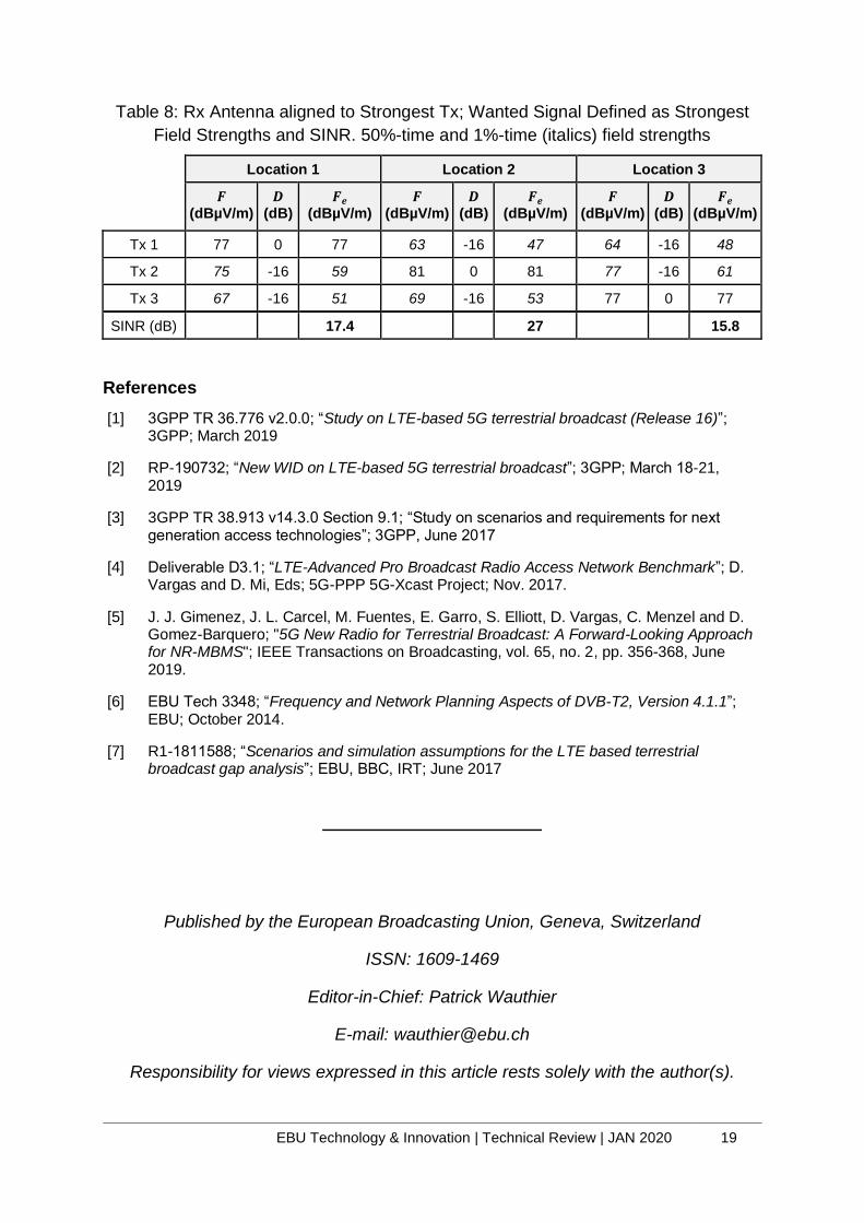
A3 Rx Antenna aligned to Strongest Tx; Wanted Signal Defined

as Strongest

With this methodology, any transmitter may provide a Wanted Signal, and at each

location the receiving antenna is aligned to the transmitter providing the highest

50%-time value of 𝐹. This is a significant additional degree of freedom, the effect of

which is shown in Figure 11 and Table 8, where we can now see that a positive SINR

may be achieved at all locations.

At location 1 the wanted transmitter remains Tx 1, which continues to provide an

SINR of 19.4 dB as there is no better direction in which to align the receiving

antenna.

At location 2 it is now possible to align the receiving antenna with Tx 2 and define this

transmitter as the wanted. Doing so increases the effective field strength from this

transmitter while simultaneously reducing the interfering signal from transmitter 1.

The SINR at this location rises to 27 dB, up from 1.6 dB in the previous example.

Similarly, at location 3 it is now possible to align the receiving antenna to Tx 3 and

define transmitter 3 to be the wanted. The SINR at this location therefore rises

from -3.1 dB to 15.8 dB, even though it remains at location 3.

This methodology produces a significantly higher SINR than the other two methods

considered above.

Highest value of 𝐹 at locations within the pixel Corresponding value of 𝐹𝑒

Figure 11: Strongest Transmitter Method


Table 8: Rx Antenna aligned to Strongest Tx; Wanted Signal Defined as Strongest

Field Strengths and SINR. 50%-time and 1%-time (italics) field strengths


𝑭 (dBµV/m)

𝑫 (dB)

𝑭𝒆 (dBµV/m)

𝑭 (dBµV/m)

𝑫 (dB)

𝑭𝒆 (dBµV/m)

𝑭 (dBµV/m)

𝑫 (dB)

𝑭𝒆 (dBµV/m)

Tx 1 77 0 77 63 -16 47 64 -16 48

Tx 2 75 -16 59 81 0 81 77 -16 61

Tx 3 67 -16 51 69 -16 53 77 0 77

SINR (dB) 17.4 27 15.8

References

[1] 3GPP TR 36.776 v2.0.0; “Study on LTE-based 5G terrestrial broadcast (Release 16)”; 3GPP; March 2019

[2] RP-190732; “New WID on LTE-based 5G terrestrial broadcast”; 3GPP; March 18-21, 2019

[3] 3GPP TR 38.913 v14.3.0 Section 9.1; “Study on scenarios and requirements for next generation access technologies”; 3GPP, June 2017

[4] Deliverable D3.1; “LTE-Advanced Pro Broadcast Radio Access Network Benchmark”; D. Vargas and D. Mi, Eds; 5G-PPP 5G-Xcast Project; Nov. 2017.

[5] J. J. Gimenez, J. L. Carcel, M. Fuentes, E. Garro, S. Elliott, D. Vargas, C. Menzel and D. Gomez-Barquero; "5G New Radio for Terrestrial Broadcast: A Forward-Looking Approach for NR-MBMS"; IEEE Transactions on Broadcasting, vol. 65, no. 2, pp. 356-368, June 2019.

[6] EBU Tech 3348; “Frequency and Network Planning Aspects of DVB-T2, Version 4.1.1”; EBU; October 2014.

[7] R1-1811588; “Scenarios and simulation assumptions for the LTE based terrestrial broadcast gap analysis”; EBU, BBC, IRT; June 2017

Published by the European Broadcasting Union, Geneva, Switzerland

ISSN: 1609-1469

Editor-in-Chief: Patrick Wauthier

E-mail: [email protected]

Responsibility for views expressed in this article rests solely with the author(s).

receiving antenna alignment in hexagonal grid simulations: a … · receiving antenna alignment...

Documents