reasoning with belief functions: an analysis of …ftp.cs.ucla.edu/pub/stat_ser/r136.pdfreasoning...

Reasoning with Belief Functions: An Analysis

of Compatibility Judea Pearl

Computer Science Department, UCLA, Los Angeles, California

ABSTRACT

This paper examines the applicability o f belief functions methodology in three reasoning tasks: (1) representation of incomplete knowledge, (2) belief updating, and (3) evidence pooling. We find that belief functions have difficulties representing incomplete knowledge, primarily knowledge expressed in conditional sentences. In this context, we also show that the prevailing practices of encoding if-then rules as belief function expressions are inadequate, as they lead to counterintuitive conclusions under chaining, contraposition, and reasoning by cases. Next, we examine the role of belief functions in updating states of belief and find that, i f partial knowledge is encoded and updated by belief function methods, the updating process violates basic patterns o f plausibility and the resulting beliefs cannot serve as a basis for rational decisions. Finally, assessing their role in evidence pooling, we find that belief functions offer a rich language for describing the evidence gath- ered, highly compatible with the way people summarize observations. However, the methods available for integrating evidence into a coherent state of belief ca- pable of supporting plausible decisions cannot make use of this richness and are challenged by simpler methods based on likelihood functions.

KEYWORDS: belief funct ions, Dempster-Shafer theory, knowledge and evidence, nonmonotonic reasoning, conditional information

1. INTRODUCTION AND A BRIEF REVIEW

In earlier publications (Pearl [27, 28]) I attempted to uncover the epistemo- logical basis of the Dempster-Shafer belief functions (BF), so as to form a meaningful assessment of their applicability vis-a-vis the Bayesian approach.

Address correspondence to Judea Pearl, Computer Science Department, UCLA, Los Angeles, CA 90024-1596.

International Journal of Approximate Reasoning 1990; 4:363-389 ~) 1990 Elsevier Science Publishing Co., Inc. 655 Avenue of the Americas, New York, NY 10010 0888-613X/90/$3.50 363

3(14 Judea Pearl

With the help o f a canonical model cast in terms of "probabilities o f provability," I then identified some basic issues that must be addressed if the theory is to provide a viable formalism for evidential reasoning. The purpose o f this paper is to provide an updated examination o f these issues in light of recent discussions I have had with colleagues and coworkers, and in light of new observations made subsequent to these discussions.

1.1. Knowledge, Belief, and Evidence

To facilitate our discussion of belief functions and their applications, I will adopt the following distinction between knowledge, belief, and evidence. Knowledge encodes judgments about the general tendency of things to happen, evidence summarizes the impact o f that which actually happened, whereas belief combines the two--it consists of assertions about a specific situation inferred by applying generic knowledge to a set o f evidence sentences. 1 For example, the sentence "Birds fly" encodes knowledge about the general tendency of birds to enjoy flying capabilities. The sentence "Tweety is a bird" provides an evidence by summarizing certain observations made on a specific object named Tweety. The sentence "Tweety flies" represents a state o f belief about Tweety 's capabilities, based on both generic knowledge (about birds) and a specific evidence (about Tweety).

Of course, all sentences are subjective and hence could be annotated with various shades o f confidence. Note that evidence sentences and belief sentences both refer to specific situations and may rely on both generic knowledge and specific observations. The distinction between the two is that the process by which knowledge and observation were combined is made explicit in the case of belief sentences and remains implicit in the case of evidence sentences. For example, "Tweety is a bird" will be treated as an evidence sentence if it is fed as an input to a system that reasons about the habits of birds, but will be treated as a belief sentence by a system that reasons about the classification o f animals from more rudimentary observations.

1.2. The Belief Function Formalism

Belief functions result from assigning probabilities to sets rather than to the individual points, with points representing specific worlds and sets reflecting

1These definitions of knowledge, evidence, and belief correspond to the common distinction in AI systems between "domain knowledge," "ground facts," and "inferences." The distinction is made solely for the purpose of disambiguating future discussions; I do not claim that people do not possess other forms of knowledge (e.g., procedural or normative) or that they do not occasionally cross the boundaries of these definitions. I define evidence as a summary of observations, so as to allow testimonies that, instead of describing raw observations, assess the impact of undisclosed observations on questions of interest, for example, "This object is very likely to be a bird."

Reasoning with Belief Functions 365

propositions about those worlds. Given an initial probability assignment m(-) to a select set F of propositions (called focal elements), namely,

E m(B) = 1, m(B) >_ 0 (1) B E F

every proposition in the language then acquires a pair of measures, Bel(.) and PI(.), such that

Bel(A) = E m(B) (2) B implies A

and PI(A) = 1 - BeI(-~A)

Any measure Bel(.) constructed in such a manner is called a belief function, and its associated measure PI(-) is called plausibility.

A necessary and sufficient condition for a function Bel(.) to be a belief function is that it satisfies

and

Be l (~ ) - -0 , Bel(A V ~A) = 1

Bel(AI V ..- VAn) > ~ B e l ( A i ) - ~ B e l ( Z i AAj) + . . . . (3) i i < j

A l, A2 . . . . . An being any collection of propositions. Given two belief functions Bell and Bel2, their orthogonal sum Bell ® Bel2,

also known as Dempster's rule of combination, is defined by their associated probability assignments

(ml •m2)(A) = K E ml(A1)m2(A2), A ~ f~ (4) A1 AA2=A

where

K-1 = E ml(A1)m2(A2) (5) Al A A 2 ¢ ~

The operator ~3 is known to be commutative and associative. As a special case of Eq. (4), if m2 establishes the truth of proposition B,

that is, m2(B) = 1, then the combined belief function becomes

Bell (A V ~B) - Bell (~B) Bell ( A [B) = 1 - Bell (~B) (6)

This formula is known as Dempster's conditioning.

366 Judea Pearl

A belief function is called additive or Bayesian if each of its focal elements is a singleton, that is, an elementary event or a possible world. Bayesian belief functions satisfy Bel(A) = PI(A) = 1 -BeI (~A) . If Bell is Bayesian, then Bell ~3 Bel2 is also Bayesian, and Dempster's conditioning reduces to ordinary Bayesian conditioning (Shafer [30]).

1.3. The Methodology of Belief Functions

The methodology according to which belief functions have been applied to reasoning problems consists of three separate components:

1. Representation of incomplete knowledge. In cases where fully specified probabilistic knowledge is not available, belief functions are often used to represent states of partial knowledge, with Bel(A) interpreted as a strength of arguments in favor of A. The input information is often elicited by assessing the highest probability one is willing to commit to A and to its complement ~A, and encoding these assessments as re(A) and m(-~A), respectively.

2. Belief updating. Belief functions offer a method of assimilating the impact of new evidence into a state of partial knowledge or partial belief. If the initial state is encoded as a belief function Bel(-) and the evidence as a belief function Bele (.), then the updated state of belief Bel'(.), accounting for the impact of the new evidence, is given by Dempster's combination Bel I = Bel ~3 Bele.

3. Pooling of evidence. When multiple pieces of evidence are available, the BF combination method provides a faithful summary of the information carried by all the individual pieces. The method consists of encoding each piece of evidence as a belief function and combining these functions by Dempster's rule of orthogonal sum. Dempster's rule, Eq. (4), reflects two assumptions about evidence combination: a. Independence. Successive pieces of evidence are independent of each

other. b. Renormalization. Whenever two pieces of evidence impart weights to

contradictory propositions [A1 A A2 = ~ in Eq. (4)], that weight is redistributed among the noncontradictory propositions, proportionally to their weights.

In subsequent discussions I will deal separately with these three components of BF methodology. In Section 2, I will examine whether the representational scheme offered by BF adequately represents common types of incomplete knowledge. In Section 3, I will focus on those cases where the BF representation is adequate, and will evaluate its belief-updating component. My conclusions (Section 4) are that belief functions have serious difficulties serving in these two functions, and their potential of serving in the third function, evidence pooling, is limited to cases where the evidence thus pooled will ultimately be used to


update an ordinary (i.e., additive) probability measure or a purely categorical knowledge state. First (Section 1.3), I would like to recount an interpretation of belief functions that I have found helpful in understanding the workings of the theory and its potential applications.

1.4. A Probabifistic Interpretation of Belief Functions

Historically, belief functions were first interpreted as lower and upper probabilities induced by a special family of probability distributions (Dempster [7]). Each member of the family represents a redistribution of the sets' probabilities m(-) to individual points within those sets, and each (Bel(A), PI(A)) pair provides bounds on the " t rue" probability of A. This interpretation, still a favorite of many researchers (Kyburg [20], Fagin and Halperu [11]), is unsatis- factory when it comes to evidence combination; the correspondence between the constituent families of probabilities and the family resulting from Dempster 's rule defies a natural explanation (see Section 3.1). Shafer's [30] interpretation of Dempster 's theory abandons the idea that belief functions arise as lower bounds of a family of ordinary probability distributions; rather, it views belief functions as a natural representation of English words such as "belief ," "doubt ," "evidence," and "suppor t , " ' and Dempster 's rule of combination as the fundamental step in reasoning about uncertain evidence. In Shafer's view, "bel ief" in a hypothesis does not measure the chance that it is true, but rather the strength of the arguments we have in favor of the hypothesis.

In translating Shafer's view into the language of logic, using the notions of proofs and constraints (or axioms), it becomes clear that belief functions are none other than probabilities ofprovability (Pearl [27], p. 423). In other words, BeI(A) stands for the probability that the constraints imposed by the available evidence, together with the constraints that normally govern the domain, will be sufficient to compel the truth of A and exclude its negation. Formally, we are given a collection of logical theories, T1 . . . . . Tn, each logical theory is characterized by a set of formulas called axioms, and each theory is assigned a probability Pi such that the probabilities sum to 1. The belief in a formula A is the sum of the probabilities of the theories from which A follows as a logical consequence. 2 (I am indebted to Fagin and Halpern [11] for this succinct wording.) This interpretation has the advantage that Bel(A) no longer represents properties of some nebulous family of probability functions but rather an ordinary probability of a bona fide event--the existence of a log-

2Each theory corresponds to one focal element B in (1), and its probability P~ corresponds to m(B). If one associates with each theory the set of worlds (or models) consistent with its defining axioms, the resulting theorems can be described as a system of random sets (Nguyen [25]). Our notion of "provability" is semantical, resting on logical consequences, to be distinguished from syntactical proofs, which are normally embedded in a specific axiomatizntion.

368 Judea Pearl

ical proof for A. The reason that this event is random is that the set of axioms from which the proof is to be assembled is not known with certainty, only with probability. Note that both a formula and its negation might have belief 0, since neither might follow from any of the theories.

This interpretation of belief functions now provides a simple semantics for Dempster's rule of evidence combination, Eq. (4). Each piece of evidence, say el and e2, defines a probability mass over a collection of theories, and the combined evidence el • e2 likewise defines a probability mass over a collection of joint theories. Each joint theory is made up of a union of two axiom sets, one taken from e~ and one from e2. The mass assigned to such a union is the product of the individual masses (thus reflecting evidence independence), while the mass attributed to any contradictory theory is redistributed among the noncontradictory theories in proportion to their weights. Thus, the belief function resulting from this combination rule is simply the conditional probability o f provability, given that the two pieces of evidence are noncontradictory.

The advantage of this interpretation is that it enables us to discuss in meaningful terms whether Dempster's rule is applicable: namely, whether in the context of a specific domain it is meaningful to condition beliefs on the evidence being noncontradictory. Shafer's canonical model of random codes (Shafer [32]) is an example of a context where the assumption of noncontradictory evidence is a reasonable one to make. Here messages were presumed to originate from a consistent source, and so the event of two deciphered messages yielding two incompatible conclusions can be ruled out as a physical impossibility.

What remains unjustified in this example is why we should concern ourselves with "the probability that the evidence implies A " (Shafer [32]) rather than the probability that A is true given the evidence. Motivating this computation is one unresolved difficulty with the semantics of belief functions. For example, in circuit diagnosis we normally ask for the probability that a particular component is faulty, not that it must be faulty for lack of another explanation. Taking the latter as a basis for decisions might yield undesirable policies of testing or replacing faulty components. The lack of justification for this component in Shafer's random code example was also criticized by Good [15] and Levi [22], and more of its consequences will be discussed in Section 3.2.

However, there are situations where it is indeed the probability of necessity and possibility that we wish to ascertain, rather than that of truth, and it is within such situations that we should seek canonical examples for the construct of belief functions. Suppose, for example, we are scheduling a construction project, and our body of evidence consists of a set of estimates ml, m 2 , . . . , ran, where each mi stands for the chance that resource ri will become unavailable during the construction. In this context, it is not uncommon to inquire as to the probability that a certain decision (say changing a design option) will have to be made out of a compelling necessity, for lack of any viable alternative, rather than the probability that it will actually be made, as an option of choice or convenience.


Unfortunately, evidence inconsistency in this context means the impossibility of meeting all scheduling constraints, not a physical impossibility, and cannot be ruled out a priori as in the diagnostic problems discussed earlier. Thus, it would not be justified to apply Dempster's nile of combination in such applications.

My attempts to find natural applications for belief functions have encountered the following pattern. In tasks of synthesis and prediction, where we sometimes have reasons for computing the probability of necessity (e.g., the scheduling problem), we normally find no justification for assuming evidence consistency. In tasks of diagnosis or abduction, where we normally find justification for assuming evidence consistency (e.g., Shafer's random code or the Three Pris- oners puzzle, Section 3.1), we can find little justification for computing the probability of necessity. The only example I found that motivates both components together and thus reflects precisely the quantity computed by Bel is the retrospective version of the scheduling problem, where, years after the comple- tion of the project, one asks: "What is the probability that a certain decision had to be made out of absolute necessity?" or, alternatively, "What is the probability that the person in charge knew that a certain event must have occurred, out of logical necessity?"

2. DO BELIEF FUNCTIONS FACILITATE AN ADEQUATE REPRESENTATION OF INCOMPLETE KNOWLEDGE?

By "incomplete knowledge" I mean knowledge that is insufficient for fully specifying a probability distribution over the set of possible worlds. Indeed, the most appealing feature of BF vis-h-vis the Bayesian approach has been that the latter requires the full specification of a joint distribution function over the variables in the domain while "using belief functions, one need not estimate any probabilities that are not readily available" (Strat [36]). Thus, if only some probabilities are known, but not all, one obvious semantics of our knowledge would be an implicit family of probability functions, a family that contains all functions that comply with what we know but makes no commitment relative to what we do not know. Alternative semantics are also possible (e.g., the maximum-entropy approach), according to which the missing probabilities can be recovered. In this section I will discuss the relationships between belief functions and families of distributions that reflect naturally occurring cases of incomplete knowledge. The discussion should also be relevant to those who disavow any relation between belief functions and uncertain probabilities (e.g., Shafer [31]), because the emphasis will not be on whether belief functions can represent such families with full numerical precision but on whether the two representations can adequately capture the meaning intended by the knowledge provider.

370 Judea Pearl

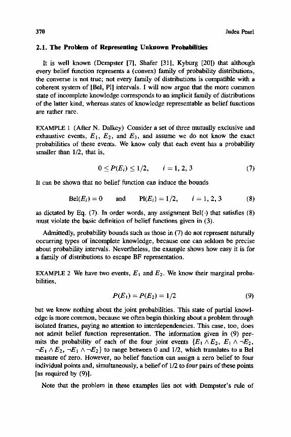
2.1. The Problem of Representing Unknown Probabilities

It is well known (Dempster [7], Shafer [31], Kyburg [20]) that although every belief function represents a (convex) family of probability distributions, the converse is not true; not every family of distributions is compatible with a coherent system of [Bel, PI] intervals. I will now argue that the more common state of incomplete knowledge corresponds to an implicit family of distributions of the latter kind, whereas states of knowledge representable as belief functions are rather rare.

EXAMPLE 1 (After N. Dalkey) Consider a set of three mutually exclusive and exhaustive events, E l , E2, and E3, and assume we do not know the exact probabilities of these events. We know only that each event has a probability smaller than 1/2, that is,

0 <_ P(Ei) <_ 1/2, i = 1, 2, 3

It can be shown that no belief function can induce the bounds

(7)

Bel(Ei) -- 0 and PI(Ei) = 1/2, i = 1, 2, 3 (8)

as dictated by Eq. (7). In order words, any assignment Bel(.) that satisfies (8) must violate the basic definition of belief functions given in (3).

Admittedly, probability bounds such as those in (7) do not represent naturally occurring types of incomplete knowledge, because one can seldom be precise about probability intervals. Nevertheless, the example shows how easy it is for a family of distributions to escape BF representation.

EXAMPLE 2 We have two events, El and E2. We know their marginal probabilities,

P(E1) = P(E2) = 1/2 (9)

but we know nothing about the joint probabilities. This state of partial knowledge is more common, because we often begin thinking about a problem through isolated frames, paying no attention to interdependencies. This case, too, does not admit belief function representation. The information given in (9) per- mits the probability of each of the four joint events {El A E2, El A-~E2, ~E1 AE2, ~E1 A ~E2} to range between 0 and 1/2, which translates to a Bel measure of zero. However, no belief function can assign a zero belief to four individual points and, simultaneously, a belief of 1/2 to four pairs of these points [as required by (9)].

Note that the problem in these examples lies not with Dempster's rule of


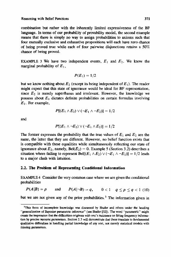
combination but rather with the inherently limited expressiveness of the BF language. In terms of our probability of provability model, the second example means that there is simply no way to assign probabilities to axioms such that four mutually exclusive and exhaustive propositions will each have zero chance of being proved true while each of four pairwise disjunctions retains a 50% chance of being proved.

EXAMPLE 3 We have two independent events, E1 and E2. We know the marginal probability of E l ,

P ( E I ) = 1/2

but we know nothing about E2 (except its being independent of El ). The reader might expect that this state of ignorance would be ideal for BF representation, since E2 is merely superfluous and irrelevant. However, the knowledge we possess about El dictates definite probabilities on certain formulas involving E2. For example,

P[(E1 AE2) V (~El A ~E2)] ---- 1/2

and

P[(E1 A ~ g 2 ) V (-~E1 AE2)] = 1/2

The former expresses the probability that the true values of E1 and E2 are the same, the latter that they are different. However, no belief function exists that is compatible with these equalities while simultaneously reflecting our state of ignorance about E2, namely, Bel(E2) -- 0. Example 5 (Section 3.2) describes a situation where failing to represent Bel[(El A E2) V (~E1 A ~E2)] ---- 1/2 leads to a major clash with intuition.

2.2. The Problem of Representing Conditional Information

EXAMPLE 4 Consider the very common case where we are given the conditional probabilities

P(AIB)= p and P(AI~B)=q, O < l - q < _ p < q < l (10)

but we are not given any of the prior probabilities. 3 The information given in

3This form of incomplete knowledge was discussed by Shafer and others under the heading "generalization of Bayesian parametric inference" (see Sharer [32]). The word "parametric" might create the impression that the difficulties originate with one's insistence on fitting frequency information by precise numeric parameters. Section 2.3 will demonstrate that these translate to fundamental qualitative difficulties in handling partial knowledge of any sort, not merely statistical models with missing parameters.

372 Judea Pearl

(10) induces several constraints on the probabilities of other propositions in this frame, including, for example,

0 <_ P(A AB) < p

p < P(A) <_ q

1 - q < P[(A A B) V (-~A A ~B)] _< p

Again, no belief function exists that matches these upper and lower probabilities without violating the basic conditions in (3).

I consider this latter example to be a major shortcoming of BF theory. Condi- tional information is, in my opinion, the basic building block in the organization of human knowledge. It is this information that enables us to sort experiences and store them in the right context, with the conditioning propositions (context or reference classes as they are sometimes called) serving to identify the conditions under which the future use of this experience would be appropriate. It is for that reason that conditional sentences 4 are so common in natural discourse and if-then rules are so popular in the design of AI reasoning systems. Therefore, it is a common practice to find an expert feeling very strongly about conditional probabilities (e.g., that a given symptom will accompany a given disease) while having no feeling at all about the priors. Unfortunately, this type of incomplete knowledge cannot be captured by belief functions.

The source of this weakness lies deep in the very nature of BF theory. Recall that the theory rests on assigning probabilities to sets of logical formulas (i.e., theories). Thus BF is essentially a theory of randomized monotonic logic, and, like every monotonic logic, it lacks a mechanism equivalent to conditioning with which context dependencies can be encoded. Indeed, it is well known that the information conveyed in a conditional probability statement

P(A [B) = p

cannot be represented by assigning probabilities to some Boolean function of A and B or to any set of Boolean formulas (Lewis [23], Goodman [16]).

Example 4 demonstrates that if our knowledge consists of conditional probabilities and we are missing the necessary priors, this knowledge cannot be adequately represented as a belief function. However, even if we are given the

'*By conditional sentences I mean utterances such as "Birds fly," "Fire causes smoke," "Smoke suggests fire," "When it rains, it pours ," and many others, that do not concern frequency information as in "Most of the people in Lawrence are white." Although the word " i f " is not mentioned explicitly, the common denominator is that the assertions made by such sentences are context- dependent; they are applicable to a narrow context circumscribed by the conditioning phrase. It is the encoding of such sentences that we examine in this example.


priors, the problem of inadequate representation might arise as soon as some conditional probabilities are missing f rom the model. The reason is that if our knowledge is organized hierarchically, then the conditional probabilities at one level of the hierarchy determine the priors of the next level, where the problem demonstrated by Example 4 might recur.

Other types of partial knowledge that render BF encoding cumbersome, if not impossible, or comparative ratings of probabilities and qualitative conditional independence relationships. For example, suppose we are given the information that P ( A A B) is at least twice as large as P ( A A C) and that A and B are independent given C. Can this information be encoded as belief functions? We know of no effective procedure for deciding such questions. Currently, the only procedure for determining the existence of belief function representation is the inequality of Eq. (3), which is computationally infeasible because it requires the enumeration of all bounds that follow from the database. Can the information be approximated by belief functions while preserving its conceptual intent? I know of no research attempting to answer such questions.

2.3. The Material Approximation

The reader may wonder at this point how BF practitioners, lacking a conditioning facility with which to express inexact if-then rules, have nevertheless managed to construct rule-based expert systems. It turns out that the prevailing practice in these systems has been to represent the rule " I f A then B " by the material implication formula A 3 B (- - -,A V B) and assign to this formula some weight w that purports to measure the strength of the rule or its validity, thus converting the rule into a bona fide belief function satisfying m(A ~ B) = w. This practice is not entirely without merit. For example, combining the re- suiting belief function with the evidence A = true does give the expected result Bel(BIA) = w. Moreover, if we are given a full specification of a joint probability, say in the form of a causal network (Pearl [27]), we can replace every conditional probability P ( x Icauses-of-x) = q by its material implication counterpart m(causes-of-x 3 x) -- q and combine these m(-) functions using Dempster ' s rule, and the result would be a bel ief function that is equivalent to the original probability model. The problems begin when the probability model is incomplete and some of the conditional probabilities (or the priors) are missing. In such cases, the material implication scheme may yield very undesirable effects, three examples of which are shown next. 5

5Another method of encoding conditional rules was proposed by Smets [35] and named conditional embedding. The idea is to represent each given rule by the least committed belief function Belo that satisfies Bel(A IB) = w and then combine the Belo functions by Dempster's rule. By "least committed," he means that of all possible belief functions, Belo allocates the least possible value for every proposition. This approximation, as well as others (Eddy and Pei [10]), have apparently not been as popular among practitioners as the material implication. Nevertheless, the difficulties demonstrated in this section apply to both.

374 Judea Pearl

CHAINING The facility of chaining inferential links, sometimes known as tran- s i t iv i ty , is inherent to rules expressed as material implication formulas; from A D B and B 3 C there follows A ~ C. When uncertainties are attached to such rules, the conclusion A ~ C is weakened but still obtains a positive measure of support (equal to the product of the supports given to the individual rules). On many occasions, however, rule transitivity must be totally suppressed, not merely weakened, or strange results will surface. One such occasion occurs in property inheritance, where subclass specificity should totally override superclass properties. The rule "Typically penguins don't fly" should not be weakened by adding the two rules "Penguins are birds" and "Typically birds fly," regardless of how strongly we believe in the latter two. Another occasion occurs in causal reasoning, where predictions should not trig- ger explanations; for example, "Sprinkler was on" predicts "Ground is wet," "Ground is wet" suggests "It rained," yet "Sprinkler was on" should not sug- gest "It rained." In such cases, softening the rules by probability assignments and combining them by BF methods does not produce the expected behavior (Pearl [27], pp. 447-450]; it weakens the flow of inference through the rule chain but does not bring it to a dead halt as it should.

CONTRAPOSITION The formula ~B 3 -~A is logically equivalent to A 3 B, so the two will acquire the same Bel measure in any formulation based on belief functions. Yet, in many cases we are ready to accept the rule " I f A then B " but are unwilling to accept " I f no t -B then n o t - A . " For example, in a world that is made up primarily of birds (some of which might be sick), I am willing to accept the rule "Typically birds fly" but unwilling to accept "Typically nonflying things are non-birds," because nonflying things in this world are likely to be sick birds.

The symmetrical nature of the material implication may lead to counterintuitive inferences, 6 especially when the negation of the consequent is established by other rules and the rules convey causal relationships. Consider the rules

I ( x ) -~ P(x) : If a person is intelligent, then that person is popular.

F ( x ) --* -~P(x): If a person is fat, then that person is unpopular.

together with our cultural bias that intelligence is independent of physical ap- pearance. Now assume that each of the two rules has a strength m and we learn that Joe is fat. Formulating this information in BF terminology (using the material implication) produces the strange result that Joe is believed to be not intelligent with strength m 2. Most people would agree that it is reasonable to believe (with degree m) that Joe is unpopular, yet it is absurd to chain this

6These are further magnified when we consider criteria by which conditional rules are confirmed by empirical data (see Lewis [23] and Goodman [17]).


belief with the contraposition of the first rule and conclude (with belief m 2) that Joe is not intelligent.

REASONING BY CASES Suppose we are given the following two rules:

If A then B, with certainty 0.9.

I f norA then B, with certainty 0.7. (11)

Common sense dictates that even if we do not have any information about A we should still believe in B to a degree at least 0.7. The BF formulation does not support this intuition. I f we interpret (11) as statements of conditional probabilities, then this information cannot be represented in terms of belief functions (see Section 2.2, Example 4). If we try to force a BF encoding by interpreting the rules as material implications, we obtain BeI(B) = 0.63, in clear violation of common sense.

To appreciate the danger of casting rules as graded material implications, consider the following (hypothetical) database, rating the commitments of three religions toward observing the biblical prohibition on eating pork:

Jew(x) ~ Observe(x) (0.70)

Muslim(x) ~ Observe(x) (0.90)

Christian(x) ~ Observe(x) (0.001) (12)

Suppose we know that Joe is either a Jew or a Muslim; does he refrain from eating pork? The answer we get from the material approximation is rather strange: yes, with belief 0.63. Further yet, imagine that instead of the first rule in (12), we have a more detailed account of Jews' commitment to dietary laws, as given by the table 7

Orthodox-Jew(x) --, Observe(x) (0.999)

Conservative-Jew(x) ~ Observe(x) (0.80)

Reformed-Jew(x) ~ Observe(x) (0.40)

Nonaffiliated-Jew(x) --~ Observe(x) (0.20)

How strongly are we now willing to believe that Joe would refrain from eating pork? The answer produced by the material approximation is equal to the product of all the probabilities listed in Joe 's category, giving a minute belief of

7The numbers in this table should not be construed as reflecting statistical data but, rather, subjective assessments of the degree to which each antecedent provides an argument for the consequence.

376 Judea Pearl

only 0.0575. Thus, the more we know about Jewish customs, the less willing we are to endow Joe with any trait of Jewish tradition. 8 CAN THE MATERIAL APPROXIMATION BE IMPROVED? Strangely, despite the weaknesses demonstrated in the examples above, the material implication formulation of if-then rules still permeates the practice of BF systems (Ginsberg [14], Baldwin [2], Falkenhainer [13], D 'Ambros io [5], Lowrance et al. [24], Zarley et al. [37], Biswas and Anand [3], Laskey et al. [21], Hsia and Shenoy [19]). In some systems (e.g. , Laskey et al. [21]), special provisions are installed to prevent undesirable chaining. In others (e.g. , Ginsberg [14]), metarules are proposed to enforce specificity. This brings into question whether a theory requiring the protection of special programming fixes provides an adequate account of evidential reasoning. The difficulty is further compounded by the fact that we do not know in advance when such fixes are necessary. Given a partially specified knowledge base, we do not have any guidance for deciding whether it can be represented by belief functions or whether the material implication formulation will provide a reasonable approximation of the knowledge available.

A natural question to ask is whether the material approximation can be improved. All indications are that every BF encoding is bound to encounter difficulties similar to those shown above; the very idea of encoding if-then rules as individual belief functions to be combined by a uniform principle seems to be incompatible with the information conveyed by the rules. This can be seen from the penguin example of Section 2.3.1. Suppose we know that Tweety is both a penguin and a bird, and we wish to assess her flying capability. Any method based on belief function combination will remain oblivious to the second rule, stating that all penguins are birds. Knowing that Tweety is both a penguin and a bird renders Bel(Tweety f l ies) solely a function of rule 1, "Typical ly penguins do not fly," and rule 3, "Typical ly birds fly," regardless of whether penguins are a subclass of birds or birds are a subclass of penguins. This stands contrary to common discourse, where people expect class properties of be overriden by properties of more specific subclasses.

In conclusion, whereas it is true that "with belief functions, one need not estimate any probabilities that are not readily available" (Strat [36]), it is equally true that with bel ief functions, one cannot use some probabilities that are available, especially those embodied in if-then rules.

3. BELIEF U P D A T I N G

In this section we focus on those cases where partial kno'Tcledge does lend itself to BF encoding. In such cases the bounds provided by belief functions

SReaders preferring more "practical" examples are invited to exercise this paradox on the cholestatic jaundice example of Gordon and Shortliffe [18]. Assume that we know the tendency tl of hepatitis to develop a complication C and the tendency t2 of cirrhosis to develop C, and we wish to assess the tendency t of a patient known to be definitely suffering from intrahepatic cholestasis, that is, from either hepatitis or cirrhosis. The answer produced will be t = tit2.


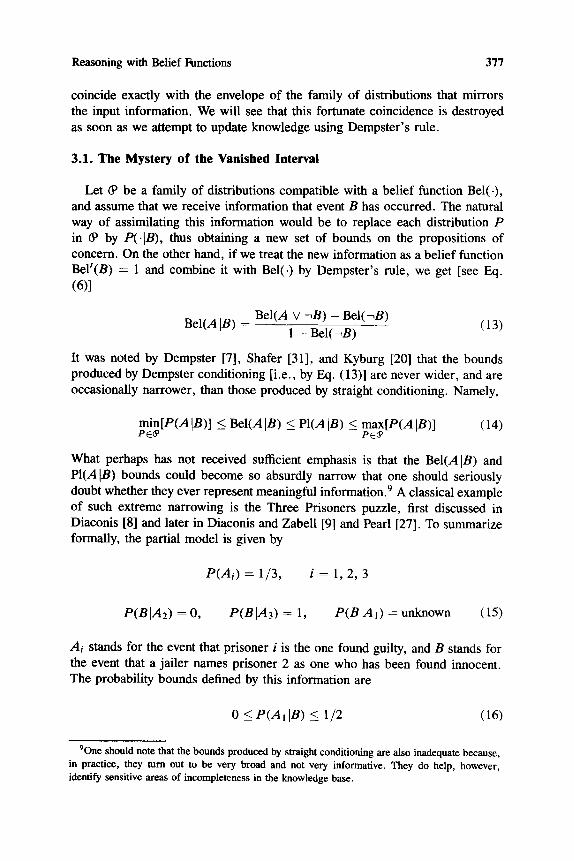
coincide exactly with the envelope of the family of distributions that mirrors the input information. We will see that this fortunate coincidence is destroyed as soon as we attempt to update knowledge using Dempster's rule.

3.1. The Mystery o f the Vanished Interval

Let 6) be a family of distributions compatible with a belief function Bel(.), and assume that we receive information that event B has occurred. The natural way of assimilating this information would be to replace each distribution P in (P by P(.IB), thus obtaining a new set of bounds on the propositions of concern. On the other hand, if we treat the new information as a belief function Bel'(B) = 1 and combine it with Bel(.) by Dempster's rule, we get [see Eq. (6)]

Bel(A I B) = Bel(A V --B) - Bel(--,B) (13) 1 - B e l ( ~ B )

It was noted by Dempster [7], Shafer [31], and Kyburg [20] that the bounds produced by Dempster conditioning [i.e., by Eq. (13)] are never wider, and are occasionally narrower, than those produced by straight conditioning. Namely,

min[P(AlB)] < Bel(AIB) < PI(AIB) < max[P(AIB)] (14) PE(P PE(P

What perhaps has not received sufficient emphasis is that the Bel(A IB) and PI(A IB) bounds could become so absurdly narrow that one should seriously doubt whether they ever represent meaningful information. 9 A classical example of such extreme narrowing is the Three Prisoners puzzle, first discussed in Diaconis [8] and later in Diaconis and ZabeU [9] and Pearl [27]. To summarize formally, the partial model is given by

P(Ai) = 1/3, i = 1, 2, 3

P(BIA2) = O, P(BIA3) = 1, P(BIA 0 = unknown (15)

Ai stands for the event that prisoner i is the one found guilty, and B stands for the event that a jailer names prisoner 2 as one who has been found innocent. The probability bounds defined by this information are

0 <_P(A~IB) < 1/2 (16)

9One should note that the bounds produced by straight conditioning are also inadequate because, in practice, they turn out to be very broad and not very informative. They do help, however, identify sensitive areas of incompleteness in the knowledge base.

378 Judea Pear

while the belief function formulation gives [taking m(Ai) --- 1/3, i = 1, 2, 3]

Bel(A 1 IB) = 1/2 = PI(A 1 IB)

Bel(A 11 ~B) = 1/2 = PI(A l I~B) (17)

This example demonstrates that by encoding a state of partial knowledge as a belief function and conditioning it on a certain body of evidence, the gap between Bel(.) and PI(-) could mysteriously disappear, thus giving the false impression that Bel(.) is based on precise probabilistic information, when such information is in fact not available. Any confidence interval interpretation one attempts to ascribe to the original belief function is destined to be very short- lived; as soon as we receive a piece of evidence, the correspondence between the original family of distributions and the one resulting from Dempster's combination might forever be destroyed. Indeed, Eq. (17) shows that the family of distributions defined by the partial model of Eq. (15) shrinks to a singleton distribution:

P(A1 AB) = 1/2, P(A3 AB) ---- 1/2

as soon as the evidence B = true is obtained. Why such an innocuous piece of evidence should bring about the total exclusion of all other distributions, perfectly consistent with the evidence, remains a total mystery.

3.2. The "Spoiled Sandwich" Effect

One can perhaps dismiss the strange phenomenon demonstrated by the Three Prisoners story and claim that the interval [Bel, P1] was never meant to represent upper and lower probabilities, but rather a new mental construct that conforms to its own norms of coherence, unshared by probabilities. I would be inclined to accept such arguments had the quantity Bel computed in (17) been reflective of some distinct linguistic expression in natural usage, or had the difficulties encountered been confined to numerical disagreements with the predictions of probability theory. Unfortunately, the difficulties go much deeper, as they clash with some universal principles of plausible reasoning having nothing to do with probabilities. One such clash is demonstrated by the "spoiled sandwich" effect, which illustrates that Bel(.) does not possess qualities we normally associate with the English word "bel ief" and brings into question whether it can ever serve as a basis for decision making.

The "sandwich" metaphor is borrowed from Aleliunas [1] to describe the following principle of plausible reasoning:

If two diametrically opposed assumptions yield two different degrees of belief in a proposition Q, then the unconditional degree of belief merited by Q should be somewhere between the two. (Pearl [27], p. 17)


It is by virtue of this principle that we agree, given the information in F_,q. (11) (Section 2.3), that B should merit a belief somewhere between 0.9 and 0.7. In general, for any proposition A and for any assumption or evidence B, we should have

Bel(A) > min[Bel(A IB), Bel(A I-~B)] (18)

This principle, unfortunately, is not satisfied by belief functions, as we have seen in the Three Prisoners puzzle; the unconditional belief was Bel(A 1) = 1/3 [see Eq. (15)], while the conditional beliefs Bel(A1 tB) and Bel(A11~B) were both 1/2 [see Eq. (17)].

The real culprit for this phenomenon is not Dempster's normalization but the very nature of Bel(A) being the probability of finding a proof for A. Under the random-theory model (Section 1.4), it is quite possible that A is not provable from any of the random theories available, thus rendering BeI(A) = 0, but if we add either B or ~B as an axiom, then A will be provable by some (though not the same) theory, thus rendering both BeI(A In) and Bel(A I~n) greater than zero. This is illustrated by the following example, where Dempster's normalization plays no role.

EXAMPLE 5 (The Peter, Paul, and Mary Sandwich) Mary challenges Peter to guess what kind of sandwich she happened to prepare for lunch that day--ham or turkey. She also promises to pay Paul $1000 if Peter guesses correctly. Peter says that, for lack of even the slightest clue, he is going to toss a fair coin and guess "ham" if it turns up heads, "turkey" if it turns up tails. Mary asks Paul if he is not anxious to know what sandwich she actually prepared, but Paul brushes her off saying that he already had lunch and that it makes no difference to him; regardless of whether it is ham or turkey, in either case he has exactly a 50% chance of winning the $1000.

Mary retorts that Paul is behaving like an incurable Bayesian, and that instead of considering the chances of winning he should be considering the chances that winning is assured by the specific evidence at hand, namely, by Peter's guessing policy. She claims that Paul's current "bel ief" of winning is, in fact, zero, because either outcome of the coin, heads or tails, would leave him with no assurance of winning. However, if he would only listen to her for a moment, his belief would immediately jump to 1/2, because knowing what kind of sandwich it is would give him a 50% assurance of winning.

Paul answers that he gets enough assurance just thinking about Mary's sandwich: " I f I have a 50% assurance assuming it is ham, and 50% assuming it is turkey, then I have a 50% assurance, period!"

Why is the sandwich principle so important for rational thinking? The answer lies, I believe, in its role as a guide to decision making and knowledge

380 Judea Pearl

acquisition. Translated to decision situations, the sandwich principle leads to the "sure-thing principle":

If the person would not prefer f to g, either knowing that the event B obtains, or knowing that the event -~B obtains, then he does not prefer f to g. (Savage [29])

Stated another way:

If a person would choose the same action for every possible outcome of an experiment, then he ought to choose that action without running the experiment.

While arguments against the universal validity of the sure-thing principle have been contrived (see e.g., Blyth [4]), these usually involve intricate situations where actions influence the outcome of the experiment. If we violate the sandwich principle, we are bound to compromise the sure-thing principle even in those cases where its validity is clear and compelling. For example, a prisoner who prefers to wait patiently for his verdict before asking a question would suddenly decide to attempt an escape regardless of whether the jailer answers " B " or "not B . "

In general, if actions are guided by the value BeI(A) accorded to some hypothesis A, any inference mechanism that violates the inequality in (18) would enable an agent to increase his perceived payoffs without actually observing the outcome of an experiment; merely verifying that the experiment was performed or just imagining the possible outcomes should suffice. Such an agent will spend precious resources chasing after useless information sources (like the jailer in the Three Prisoners story), or merely daydreaming about the existence of such sources. He will quickly become a victim of money pumping in any betting situation where useless information sources are offered for a price.

In view of this phenomenon, it is hard to see how belief functions could serve as a direct basis for rational decision making. It seems that to preserve rationality we must devise an updating rule that does satisfy Eq. (18). Alternatively, since the maladies associated with belief updating tend to get masked when it applies to additive probability distributions, we can go the Bayesian route and insist that before committing to any decision (or even to any belief), we first integrate the evidence into an additive probability distribution that reflects our prior state of belief. The next subsection discusses an attempt that follows the former alternative, while Section 4 will pursue the latter.

3.3. The Fagin-Halpern Conditioning

Fagin and Halpern (FH) [12] recently proposed a conditioning rule that avoids some of the pitfalls of Dempster's rule (similar rules have also been proposed


by De Campos et al. [6]). The FH rule reads

Bel(A A B) BeI(AIIB) = Bel(A A B ) + PI(~A AB) (19)

Like Dempster's rule, FH conditioning reduces to ordinary Bayesian conditioning when Bel(-) is an additive probability function, but, unlike Dempster's rule, it faithfully reflects the probability bounds that are produced by such conditioning. In other words, instead of the inequalities in Eq. (14), FH conditioning satisfies the equalities

max[P(hJB)] = PI(AIIB) >_ Bel(AIIB) = min[P(AlB)]. (20) PE(P PE(P

Unfortunately, although FH conditioning alleviates some of the problems encountered with belief functions, it creates new ones. First, FH conditioning is not commutative, and hence we cannot process multiple evidence sequentially upon arrival. In other words, in order to correctly produce the bounds created by the conjunction of two pieces of evidence, B1 -- true and B2 = true, we must condition Bel(.) directly on B1 A B2 and compute Bel(A liB1 A B2); we cannot compute Bel(A liB1) and then condition the result on BE.

Second, the FH rule does not specify how to integrate a body of evidence that is uncertain. If we have a belief state Bel(.) and we obtain evidence e having re(B1) = ml, re(B2) = 1 - m~, a natural way to update Bel(.) would be to take the convex mixture

BeI(A lie) = ml Bel(A lIB0 + (1 - ml) Bel(A lIB2) (21)

which represents the lower bound

min [mlP(A IB1) + (1 - ml)P(A IB2)] P E &

However, it is not clear that this update captures the intended impact of the evidence. For example, a conflicting evidence with Bt = A, B2 = ~A, and ml = 1/2 would always yield Bel(A lie) = 1/2 regardless of the prior state of belief Bel(A).

4. EVIDENCE POOLING

We have seen that belief functions are often incapable of representing partial knowledge, and in those cases where they are, they must first get converted into

382 Judea Pearl

an additive probability function before they can absorb evidence in a plausible way, so as to support rational decisions. Thus, from the three components of BF methodology--representing partial knowledge, belief updating, and evidence pooling--we are left with evidence pooling as the only subtask in which belief functions can play a useful role. 10 This raises the question of whether it is worth invoking the entire BF machinery when conventional likelihood functions can offer an adequate solution.

Consider a body of evidence e characterized by a basic probability assignment m(.), and suppose we use this evidence to update a Bayesian belief function characterized by mo(w), where each w is a singleton set (i.e., a possible world). The updated belief function is governed by

(mo @ m)(w) --- Kmo(w) E m(A) A : w E A

where K is a normalizing constant. Now assume that we were to update too(W) by Bayesian methods, that is, we regard mo(w) as the prior distribution ~r(w), and we represent the evidence e by the likelihood function

X(w) & P(elw) = ~ m(A) (22) A : w 6 A

The posterior probability, in this case, will be identical to (m0 @ m)(w), since p(w le) = Kr(w)h(w). We can map any belief function into a likelihood function using (22) and be assured that, as long as the final belief is Bayesian, this Bayesian updating would yield identical results. Moreover, given that ml( . ) maps into hi(w) and that m2(.) maps into )~2(w), we can combine hi(w) and ~,2(w) directly into )~3(w) such that ml ~3 m2 properly maps into h3(w). This is done by ordinary multiplication, ha(w) -- Xl(W)),2(w), an even simpler op- eration than the orthogonal sum required for m. Why, then, do we need the powerful machinery of belief functions, if we can accomplish the same task with likelihood functions?

True, belief functions convey more information than likelihood functions; two belief functions with totally different structures can be mapped into the same likelihood function, and their structures lost. But where is this structural information ever used? Clearly, since this information gets lost the moment it is absorbed into an additive probability function, the only way it can be used is prior to belief updating and decision making, namely, in the process of evidence pooling itself. But, in what way? A natural area of application would be that of evidence assessment and knowledge elicitation; an expert may feel

l°Fagin and Halpern [12] reached the same conclusion but, intrigued by BF's ability to mimic likelihood functions, they see wider applications for belief functions than I do.


more comfortable describing the impact of an evidence in terms of weight assignment to classes rather than to individual points (see Gordon and Shortliffe [18]). However, here too, the likelihood function approach does a fairly decent job in an amazingly simple way (see Pearl [26]). Other possibilities are to use the structural information of belief functions for tracing back sources of contra- diction and for identifying areas of incompleteness. Unfortunately, we have seen that the interval P1 - Bel does not reflect the degree of conflict in the evidence or the degree of ignorance in our knowledge. Thus, the challenge remains that of identifying how the rich mathematical structure of belief functions can be harnessed to facilitate the task of automated reasoning.

My personal assessment is that the most natural role for belief functions is to serve as a mechanism for processing evidential information prior to conversion into likelihood functions. This is based on the following observation: When a person says, "I am 50% sure that B . . . . " he does not mean to sound neutral about B but expects to convey a positive support in favor of B. Even when a person says, "I think B is true but I am only 20% sure," he still expects the listener to increase his degree of belief in B. As strange as it sounds, people use absolute probabilities to communicate instructions about probability updates! In the Bayesian language, we need to convert such update statements to likelihood functions. For example, the statement "the evidence e supports B to a degree p " would be translated [see Eq. (22)] into the likelihood ratio

L - P ( e l B ) - 1

P ( e I ~ B ) 1 - p

This translation is indirect and lacks an immediate, natural justification. In the BF language, on the other hand, the statement above is encoded directly as a basic probability assignment r e ( B ) = p . This suggests that there might be some phase of reasoning where people use belief functions, possibly in interpreting the impact of an observation, or during the mental exercise of estimating probabilities from a qualitative knowledge. It is possible that during such an exercise, which requires that exceptions and assumptions be summarized in terms of numbers, a person does indeed resort to random sampling of logical theories (Section 1.4) and computes (by stochastic simulation) the probability that a proof is found for B.

If this is so, then the BF theory could serve as a useful interface between a human probability assessor and a mechanical reasoner--a translator from collo- quial assertions about probability assignments into likelihood functions. In this view, the application of belief functions in reasoning systems would parallel the role that likelihood functions have served in statistical analysis, namely, summarizing the impact of past observations (and arguments) and organizing them for absorption into a knowledge base that is compatible with one's background information, thus serving as a basis for decision making.

Judea Pearl

5. DISCUSSION

The limitations demonstrated in this paper raise some interesting issues con- cerning the relationships between the Bayesian and BF models. First, if the BF formulation is a generalization of the Bayesian one, how can the former suffer from limitations that escape the latter? In other words, why don't we regard the conclusions reached by the Bayesian analysis as a special case of what can be obtained by the BF analysis?

The answer is that the source of the difference between the two formalisms lies in their mode of application. While every additive probability function is indeed a special kind of a belief function, the Bayesian analysis concerns not one but a family of such functions. Interpreting a rule as a restriction on a family of ordinary probability functions gives different results than interpreting the rule as a single belief function, which is the prevailing interpretation in the BF strategy. If we give up this latter convenience and, mirroring the Bayesian strategy, we venture to treat each rule as a restriction on a family of belief functions, a new calculus of belief functions might emerge that might resolve some of the difficulties noted above. However, this new calculus would no longer possess the attractive features of Dempster's rule and, additionally, would still not guarantee to yield the intended results. The reason is that the space of belief functions complying with a given constraint, say Bel(A IB) -- p , is much richer than the corresponding space of simple probability functions and might include some belief functions that exhibit undesirable features. This is a price we normally pay for generalization and needs to be further explored in the case of belief functions.

The second question relates to belief functions as a representation of evidence. In Section 4 we saw that the BF language offers a more refined representation of evidence than the ones used in the Bayesian analysis (e.g., the likelihood-ratio representation), and the question arises as to why it encounters such difficulties expressing simple items of information as if-then rules, which, presumably, also reflect and arise out of empirical evidence.

The answer lies in the distinction between knowledge and evidence and in the realization that if-then rules encode the former, not the latter. Belief functions offer a rich language for conversing about an item of evidence that has just been obtained but a rather inadequate language for describing cumulative evidence that has already been crystallized and elevated to a level of knowledge, that is, suitable for interpreting other items of evidence. In the words of Shafer and Srivastava [34]: "when we use the belief function formalism we always work with specific items of evidence" and "Statistical evidence is not, however, the kind of evidence for which the belief-function formalism is most simple and most natural." Translated into AI terminology, belief functions are not natural for representing "domain knowledge"-- generic knowledge that an expert ex-


tracts either from statistical observations or from other experts in the field, as opposed to specific items of evidence. Conditional rules such as "Birds fly," "Fire causes smoke," "Smoke suggests fire," are the basic building blocks of expert knowledge, and it is in the representation of such rules that the BF formalism finds difficulties.

This distinction between knowledge and evidence must also be made in the Bayesian framework, and its importance in reasoning systems cannot be overem- phasized, even in dealing with hard rules such as "All penguins are birds" (see Geffner and Pearl [13a]). Treating such a sentence as a generic rule that applies to all objects would yield totally different results than treating it as an item of evidence pertaining specifically to Tweety, saying " I f Tweety is a penguin then she must be a bird" (equivalently, "There is indisputable evidence that Tweety is not both a penguin and non-bird").

The Bayesian formalism offers us the fiexibility of distinguishing between these two interpretations; the former is treated as a restriction on a space of admissible probability functions, and the latter as an observation upon which the admissible functions should be conditioned. Given that Tweety is a penguin and a bird, the former treatment yields the expected conclusion that Tweety does not fly (see Pearl [27]), while the latter yields the vacuous range [0, 1], that is,

0 < P(Flies(Tweety) I Penguin(Tweety), Bird(Tweety)) <_ 1

because the added information Penguin(Tweety) D Bird(Tweety) is subsumed in the available observation Penguin(Tweety) A Bird(Tweety), and so it is un- able to exploit the information that penguins are birds.

The BF approach, unfortunately, does not distinguish items of evidence re- garding specific individuals from generic rules that reflect beliefs about all individuals, and it is for this reason that Bel(Flies(Tweety)) remains oblivious to whether penguins are a subclass of birds or birds are a subclass of penguins. It should be noted that the problems associated with the representation of rules plague the BF approach only when rules are subject to exceptions. In domains where all rules are categorical, such as in strict taxonomic hierarchies, the distinction between knowledge and evidence is unnecessary and the paradoxes uncovered in Section 3 will not surface.

6. CONCLUSIONS

The current popularity of the belief function formalism stems from two fac- tor s:

1. Its willingness to admit partial knowledge, knowledge insufficient for specifying a complete probabilistic model.

386 Judea Pearl

2. The uniform and incremental manner in which it encodes and combines partial specifications, being reminiscent of logical deduction. Each specification (say a rule) is encoded as a belief function and then combined by a uniform principle, namely, Dempster's rule of combination.

This paper raises concerns relative to the ability of belief functions to properly handle partial knowledge. Our concerns have been twofold:

1. The BF analysis computes probabilities of logical necessity rather than probabilities of truth. The former may behave contrary to expectations (relative to the notion of "measure of belief") and may not provide the desired answers in diagnostic or abductive tasks

2. The BF formalism encounters difficulties representing domain knowledge, especially class-property relationships, conditional a~ertions, and default rules. Encoding and combining such rules as belief functions may yield counterintuitive conclusions.

Shafcr (personal communication) has defined the scope of BF applications as follows: "Belief functions are useful when we can formulate evidence bearing on one question in terms of probabilities, and then relate these probabilities, through a compatibility relation, to another question." In AI terminology, this scope limits the application of belief functions to cases where domain knowledge is articulated in purely deterministic terms, using a compatibility relation. Uncertainty may characterize the impact of specific items of evidence but may not enter into the stable relationships that govern entities in the domain. Such applications include strict taxonomic hierarchies, terminological definitions, and descriptions of deterministic systems (e.g., electronic circuits) but exclude domains in which the rules tolerate exceptions (e.g., medical diagnosis, default reasoning). Conditional rules, like those discussed in Section 3, do not lend themselves to direct BF analysis, and the problem of managing incomplete probabilistic knowledge remains unresolved.

But even limiting ourselves to applications where domain knowledge is ex- pressible in categorical terms, serious thought must still be given as to whether the probabilities of provability computed by belief functions would be adequate for our purpose. Circuit diagnosis is one typical example where categorical relationships adequately describe the relations between the input and the output. However, shouldn't we really be concerned with the likelihood that a component is faulty as opposed to the likelihood that it can be proven faulty? If circuits are diagnosed by BF methods and components are replaced on the basis of the mag- nitude of Bel and P1, we are back at the mercy of the spoiled sandwich effect, which in diagnosis problems might lead to unreasonable test-and-replacement strategies. Extensive experimental and theoretical studies should be undertaken to assess the behavior of such strategies, and to understand where and how they can be implemented safely.

This paper is written in the hope that by identifying areas where BF theory should not be applied, we will improve our ability to search and find admissible


applications for the theory. As DeGroot once remarked relative to the Bayesian approach, "Like all powerful weapons, it must be used only with the utmost care and in accordance with the highest ethical standards" (see discussion following Shafer [33]). In order to use our weapons with care, we must understand their powers, dangers, and limitations.

A C K N O W L E D G M E N T S

I have benefited from discussions with many colleagues, including J. Baldwin, N. Dalkey, A. Dempster, D. Dubois, H. Geffner, J. Halpern, H. Kyburg, I. Levi, M. McLeish, H. Nguyen, G. Shafer, B. Shay, P. Smets, P. Suppes, P. Walley, and N. Wilson. This work was supported in part by National Science Foundation grant IRI-88-21a.a.a. and Naval Research Laboratory grant N00014- 894-2007.

References

1. Aleliunas, R. A., A new normative theory of probabilistic logic, Proceedings o f the 7th Biennial Conference o f the Canadian Society for Computational Studies of Intelligence (CSCSI-88), Edmonton, Alta., 1988, pp. 67-74.

2. Baldwin, J. F., Evidential support logic programming, Fuzzy Sets Syst. 24, 1-26, 1987.

3. Biswas, G., and Anand, T. S., Using the Dempster-Shafer scheme in a mixed- initiative expert system shell, in Uncertainty in Artificial Intelligence, Vol. 3 (L. N. Kanal et al., Eds.), North-Holland, Amsterdam, 1989, pp. 223-240, 1989.

4. Blyth, C. R., On Simpson's paradox and the sure-thing principle, J. Am. Stat. Assoc. 67, 364-366, 1972.

5. D'Ambrosio, B., Truth maintenance with numeric certainty estimates, Proceed- ings o f the 3rd IEEE Conference on A I Applications, Orlando, Fla., 1987, pp. 244-249.

6. De Campos, L. M., Lamata, M. T., and Moral, S., The concept of conditional fuzzy measure, Int. J. Intell. Syst., 1989.

7. Dempster, A. P., Upper and lower probabilities induced by a multivalued mapping, Ann. Math. Stat. 38, 325-339, 1967.

8. Diaconis, P., Review of "A mathematical theory of evidence," J. Am. Stat. Assoc. 78, 677-678, 1978.

9. Diaconis, P., and Zabell, S. L., Some alternatives to Bayes's rule, in Information Pooling and Group Decision Making (B. Grofman and O. Guillermo, Eds.), JAI Press, Greenwich, Conn., 1986, pp. 25-38.

10. Eddy, W. F., and Pei, G. P., Structures of rule-based belief functions, IBM J. Res. Develop. 30(1), 93-101, 1986.

3gg Judea Pearl

11. Fagin, R., and Haipem, J. Y., Uncertainty, belief and probability, Research Report RP. 619/(60901), IBM, Almaden Research Center. Short version in Proceedings, International Joint Conference in A I (IJCAI-89), Detroit, 1989, pp. 1161-1167.

12. Fagin, R., and Haipern, L Y., Updating beliefs vs. combining beliefs, Unpublished report, 1989.

13. Faikenhainer, B., Towards a general purpose belief maintenance system, Proceed- ings, 2nd Workshop on Uncertainty in AI, Philadelphia, 1986, pp. 71-76.

13a.Geffner, H., and Pearl, J., A framework for reasoning with defaults, in Knowledge Representation and Defeasible Reasoning (H. Kyburg, R. Loui, and G. Carlson, Eds.), Kluer Academic Publishers, 1990, pp. 69-87.

14. Ginsberg, M. L., Non-monotonic reasoning using Dempster's rule, Proceedings, 3rd National Conference on A I (AAAI-84), Austin, 1984, pp. 126-129.

15. Good, I. L, Discussion of "Lindley's paradox," by Glenn Shafer, J. Am. Stat. Assoc. 77(378), 325-351, 1982.

16. Goodman, I. R., A measure-free approach to conditioning, Proceedings, 3rd Work- shop on Uncertainty in AI, Seattle, 1987, pp. 270-277.

17. Goodman, N., Fact, Fiction and Forecast, Athlon, London, 1954.

18. Gordon, J., and Shortliffe, E. H., A method of managing evidential reasoning in a hierarchical hypothesis space, A I 26, 323-357, 1985.

19. Hsia, Y. T., and Shenoy, P. P., An evidential language for expert systems, in Methodologies for Intelligence Systems, vol. 4 (Z. W. Ras, Ed.), Elsevier, New York, 1989, pp. 9-16.

20. Kyburg, H. E., Bayesian and non-Bayesian evidential updating, A I 31, 271-294, 1987.

21. Laskey, K. B., Cohen, M. S., and Martin, A. W., Representing and eliciting knowledge about uncertain evidence and its implications, IEEE Trans. Syst., Man Cy- bern. 19(3), 536-545, 1989.

22. Levi, I., Consonance, dissonance and evidentiary mechanisms, in Evidentiary Value: Philosophical, Judicial, and Psychological Aspects o f a Theory (P. Gar- denfors, B. Hansson, and N. Sahlin, Eds.), Library of Theoria No. 15, C. W. K. Gleerups, Lund, Sweden, 1983, pp. 27--43.

23. Lewis, D., Probabilities of conditionals and conditional probabilities, Phil. Rev. 85(3), 297-315, 1976.

24. Lowrance, J. D., Garvey, T. D., and Strat, T. M., A framework for evidential- reasoning systems, Proceedings, 5th National Conf. on A I (AAAI-86), Philadel- phia, 1986, pp. 896-901.

25. Nguyen, H. T., On random sets and belief functions, J. Math. Anal. Appi. 65, 539-542, 1978.

26. Pearl, J., On evidential reasoning in a hierarchy of hypotheses, J. AI, 28(1), 9-15, 1986.


27. Pearl, J., Probabilistic Reasoning in Intelligent Systems: Networks o f Plausible Inference, Morgan Kaufmann, San Mateo, Cal., 1988.

28. Pearl, J., On probability intervals, Int. J. Approximate Reasoning, 2(3), 211-216, 1988.

29. Savage, L. J., The Foundations o f Statistics, Wiley, New York, 1954.

30. Shafer, G., A Mathematical Theory of Evidence, Princeton Univ. Press, Prince- ton, N.J., 1976.

31. Shafer, G., Constructive probability, Synthese 48, 1-60, 1981.

32. Shafer, G., Belief functions and parametric models, J. Roy. Stat. Soc. B 44(3), 322-352, 1982.

33. Shafer, G., Lindley's paradox, J. Am. Stat. Assoc. 77(378), 325-351, 1982.

34. Shafer, G., and Srivastava, R., The Bayesian and belief-function formalisms: a general perspective for auditing, Auditing, J. Pract. Theory, vol. 9, supplement, 1990.

35. $mets, P., Un mod61e math6matico-statistique simulant le processus du diagnostic m&lical, Doctoral dissertation, Free University of Brussels, Presses Universitaires de Bruxelles. (Cited and discussed in Shafer [32].)

36. Strat, T. M., Making decisions with belief functions, Proceedings, 5th Workshop on Uncertainty in AL Windsor, 1989, pp. 351-360.

37. Zarley, D., Hsia, Y.-T., and Sharer, G., Evidential reasoning using DELIEF, Proce~ings, 7th National Conference on A I (AAAI-88), St. Paul, 1988, pp. 205 -209.

reasoning with belief functions: an analysis of …ftp.cs.ucla.edu/pub/stat_ser/r136.pdfreasoning...

Documents