Linköping University Post Print

Real-Time View-Based Pose Recognition and

Interpolation for Tracking Initialization

Michael Felsberg and Johan Hedborg

N.B.: When citing this work, cite the original article.

Original Publication:

Michael Felsberg and Johan Hedborg, Real-Time View-Based Pose Recognition and

Interpolation for Tracking Initialization, 2007, Journal of real-time image processing, (2), 2-

3, 103-115.

http://dx.doi.org/10.1007/s11554-007-0044-y

Copyright: Springer Science Business Media

Postprint available at: Linköping University Electronic Press

http://urn.kb.se/resolve?urn=urn:nbn:se:liu:diva-39505

Journal of Real-Time Image Processing manuscript No.(will be inserted by the editor)

Michael Felsberg · Johan Hedborg

Real-time view-based pose recognition and interpolation fortracking initialization

Received: date / Revised: date

Abstract In this paper we propose a new approach to real-time view-based pose recognition and interpolation. Poserecognition is particularly useful for identifying camera viewsin databases, video sequences, video streams, and live record-ings. All of these applications require a fast pose recognitionprocess, in many cases video real-time. It should further bepossible to extend the database with new material, i.e., toupdate the recognition system online.

The method that we propose is based on P-channels, aspecial kind of information representation which combinesadvantages of histograms and local linear models. Our ap-proach is motivated by its similarity to information repre-sentation in biological systems but its main advantage is itsrobustness against common distortions such as clutter andocclusion. The recognition algorithm consists of three steps:1. low-level image features for color and local orientation

are extracted in each point of the image2. these features are encoded into P-channels by combining

similar features within local image regions3. the query P-channels are compared to a set of prototype

P-channels in a database using a least-squares approach.The algorithm is applied in two scene registration experi-ments with fish-eye camera data, one for pose interpolationfrom synthetic images and one for finding the nearest viewin a set of real images. The method compares favorable toSIFT-based methods, in particular concerning interpolation.

The method can be used for initializing pose-trackingsystems, either when starting the tracking or when the track-ing has failed and the system needs to re-initialize. Due to its

This work has been supported by the CENIIT project CAIRIS(http://www.cvl.isy.liu.se/Research/Object/CAIRIS), EC Grants IST-2003-004176 COSPAL and IST-2002-002013 MATRIS. This paperdoes not represent the opinion of the European Community, and theEuropean Community is not responsible for any use which may bemade of its contents.

M. Felsberg · J. HedborgComputer Vision LaboratoryLinkoping University, SwedenTel.: +46-13-282460Fax: +46-13-138526E-mail: mfe@isy.liu.se

real-time performance, the method can also be embedded di-rectly into the tracking system, allowing a sensor fusion unitchoosing dynamically between the frame-by-frame trackingand the pose recognition.Keywords: pose recognition, pose interpolation, P-channels,real-time processing, view-based computer vision

1 Introduction

The proposed method has been developed in context of theMATRIS project1 aimed at markerless real-time tracking ofcamera poses [40]. The MATRIS system applies a hybridtechnique for estimating the pose dynamically by fusing po-sition estimates of tracked image features2 [38,37] and iner-tia measurements [24]. For this process to start or to restartin case of failure, an initial registration of the current viewin a database is required to acquire a coarse pose estimate.The proposed method allows the registration to be achievedby pose recognition3.

Pose recognition is a special case of image recognition.Most image recognition approaches are based on either ofthe following two paradigms: Model-based recognition orview-based recognition. It is propounded in the literaturethat view-centered recognition has significant advantagescompared to object-centered models (see e.g. [18], Sect. 5).Following this line of arguments, we focus on view-basedrepresentations. View-based representations can be global,i.e., the elements of the representation depend on the wholeimage, or they can be local, where the elements of the rep-resentation only depend on a sub-region of the image. Bothkinds of representation can be either dense, i.e., all imagepixels contribute to the representation, or sparse, i.e., onlyselected image pixels contribute.

The problem that we consider in this paper is the fol-lowing: Interpolate the camera pose for a previously unseen

1 http://www.ist-matris.org2 By features we denote ”a numerical property” [14].3 By recognition we denote ”identification” aka ”the process of as-

sociating some observations with a particular instance [...] that is al-ready known” [14].

2

view with a system which has seen the scene from differentposes before. Interpolation of camera poses results in a non-linear mapping on the space of previously seen images. Thedifference to view based object recognition, see e.g. [12], isthat object recognition aims at producing the most probableobject class independent of the view angle, whereas in thepresent paper, we try to estimate the camera pose as accu-rate as possible. The different views might originate from asingle physical scene (’object class’) or from several ones.

The solution that we propose belongs to the category ofdense, local methods, i.e., all image pixels contribute to theview representation, but each element has a local region ofsupport. Algorithms that work with local image regions arepopular, see e.g. [1,2], due to their ”robustness to geometricdistortion” [2]. The proposed method uses P-channels as aview representation, a relatively new technique [11] whichis related to local histograms and is introduced in Sect. 2.3.The proposed recognition algorithm consists of three steps:

1. low-level image features for color and local orientationare extracted in each point of the image

2. these features are encoded into P-channels by combiningsimilar features within local image regions

3. the query P-channels are compared to a set of prototypeP-channels in a database using a least-squares approach.

The last step is related to comparing local density estimatesof the low-level features, as a local density estimate can beobtained from a linear combination of P-channels [12]. Ithas been shown in [12] that using least-squares techniquesworks slightly better than the (regularized) Kullback-Leiblerdivergence [7] of the kernel density estimate.

The least-squares method for estimating the camera posefrom P-channels is the main contribution of this paper, i.e.,the paper focuses on the view representation and its match-ing. In order to build a system including a large databaseof stored view representations, the data has to be organizedcleverly, e.g. in tree structures, for achieving fast access, butthis is considered as a separate problem not treated in thispaper. The interested reader is referred to prominent papersas, e.g., [30,34,33].

If pose recognition shall be applied for tracking re-initial-ization of video streams and live recordings, the method mustwork in video real-time, i.e., recognition in images with PALresolution at 25 Hz, in order to avoid frames without poseestimates. For databases and video sequences, even higheraverage recognition speed might be desirable in order toanalyze the data in sub-real-time. Real-time processing onup-to-date computer systems or on future wearable systemsrules out current implementations of many powerful approaches for recognition, e.g., learning-based methods as [35,36,29], image matching [6], group-theoretic global meth-ods [13], and eigen-space projections [41]. The proposedmethod for pose recognition runs in real-time on ordinarypersonal computers.

As we cannot guaranty that all views required for suc-cessful recognition of all poses are available prior to thetracking, it must be possible to add new views, e.g. from

successful tracking, dynamically to the learning set. Requir-ing that learning has to be done on the fly excludes batch-learning methods as, e.g., [22,32]. Our proposed method al-lows to add new view representations at any time.

For a method to be applicable in practice, it needs to berobust and stable. By robustness we refer to the property of asystem or method to handle quantitative and qualitative de-viations from the assumed model, e.g., occlusion or specularhighlights. If an input to the system lies outside the modeledspace, it should lead to some standard output, e.g. suppres-sion of an input or re-initialization of a tracking system incase of lost tracking. To differentiate from general robust-ness, statistical robustness denotes the limited quantitativeinfluence of input outliers to the output of an estimation pro-cess. We consider statistical robustness as a special case ofgeneral robustness, starting from the assumption of a linearmodel for the estimator which is then modified to achievesaturation of the estimate error for outliers.

Robustness is often mixed up with the term stability, bywhich we denote bounded output error for a bounded inputerror (bibo stability), or equivalently a finite operator norm.The latter is trivially fulfilled for finite linear operators. Theproposed method is robust against intensity changes, i.e.,we do not model intensity invariance, but the system’s out-put is not influenced by changes caused by opening / clos-ing blinds, changing the aperture or shutter time. The poseestimates are robust against occlusion and specular high-lights, which is shown in the experimental section. Finally,the method behaves stable under geometric distortions, i.e.,introducing small geometric distortions leads to small addi-tional errors in the pose estimate.

In the experiments section of the paper it is shown that P-channel representations perform well compared to state-of-the-art descriptors. Many recently published visual recog-nition methods make use of SIFT features [30] in one orthe other way. The SIFT feature is computed by extractingthe SIFT (keypoint) descriptor at SIFT keypoints with ap-propriate orientation and scale. P-channels can likewise becomputed in a local frame [27] and therefore it makes senseto compare the SIFT descriptor (cf. Sect. 6 of [30]) to theP-channel representation. The SIFT descriptor is similar toa linear-spline channel representation (cf. [10]) of the gra-dient orientation weighted by the saturated gradient magni-tude. The main differences of the here applied P-channelsto SIFT descriptors are: disregard for the gradient magni-tude, no spatial weighting, inclusion of hue and saturation,and finally using piecewise polynomials of order zero andone instead of linear interpolation. SIFT descriptors of thesame dimensionality are significant slower to compute thanP-channels. Comparing the descriptive power of both im-age descriptors shows that P-channels perform equally wellfor nearest-neighbor matching and perform superior for theleast-squares interpolation of poses, i.e., non-linear mappingson the image space.

3

2 Density Estimation by Channel Representations

In this section, we recapitulate those definitions and prop-erties of channel representations which are relevant for theapplication of density estimation. Within the field of densityestimation, we only consider the simplest case where we es-timate the pdf from samples ξ j drawn from the distributionp(ξ ) using the kernel B as

p(ξ ) =1J

J

∑j=1

B(ξ !ξ j) . (1)

It is well known that the expectation value of the estimate isgiven as the convolution of the true density with the kernelfunction [3]:

E{p} = B" p . (2)

For further details and properties the interested reader is re-ferred to standard text books as e.g. [3,4]. In this section weintroduce a method for non-parametric density estimation,which is significantly faster than standard kernel density es-timators.

2.1 Channel Representations

The approach for density estimation that we will apply inwhat follows, is based on the channel representation [19,39]. The channel representation is related to observationsfrom biological systems, where receptive fields are spatiallylocated and are only sensitive to certain value ranges, e.g.colors or orientations. The spatial support and value sensi-tivities are overlapping and establish a smooth transition be-tween neighbored fields. Each receptor thus counts incom-ing stimuli weighted by the spatial distance to its center andweighted by the distance in value domain, cf. [16], Chapt. 5.

In the channel representation, compact, smooth, non-neg-ative basis functions B, the channels, are placed regularly4

in spatial and value domain (see Fig. 1 (b) for channels inthe value domain). A single measurement is defined by itsposition and value, i.e., it is considered as a point in thejoint space of position and value, and thus activates all chan-nels that have non-zero support at this point. This processis called channel encoding. Hence, a single measurementis represented by a tuple of numbers, the channel vector.Each component of this vector, i.e., each channel value, cor-responds to the activation of the respective channel.

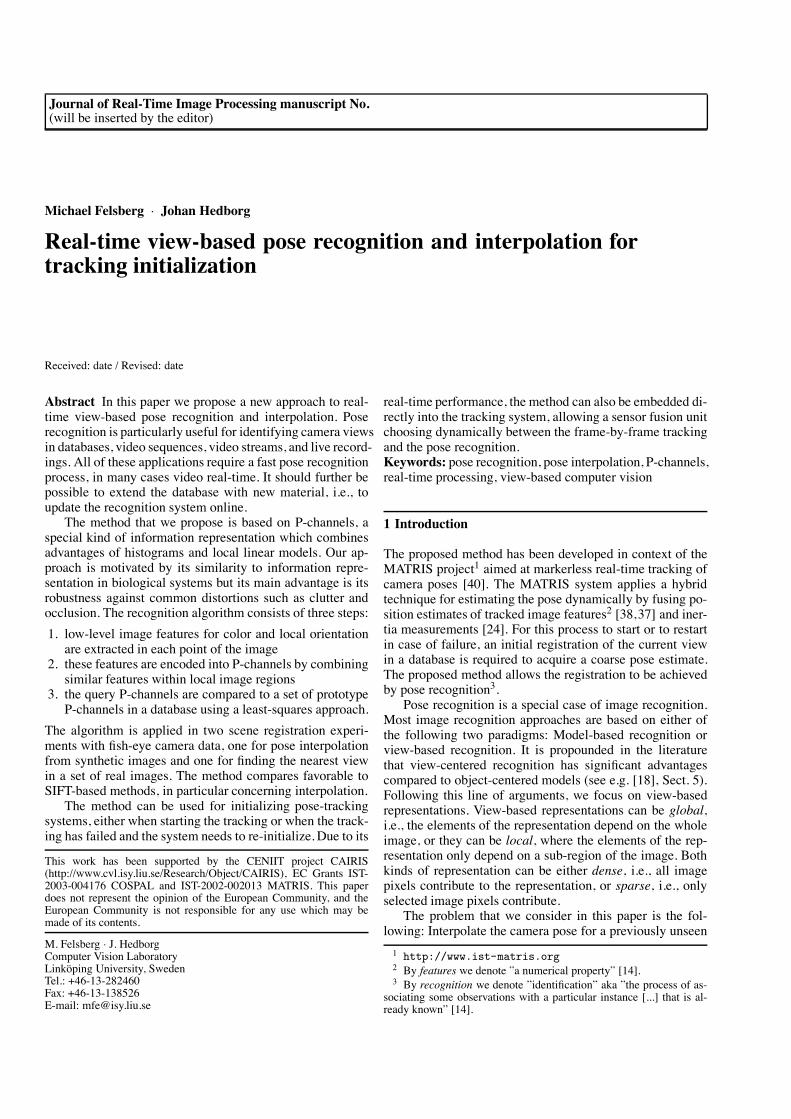
This is a highly redundant representation unless severalmeasurements drawn from the same distribution (see Fig. 1(a)) have to be represented. In that case the channel vectorsof all measurements are averaged, thus leading to a fuzzyvoting scheme [8] for the different channels (see Fig. 1 (c)).Picking local maxima of the channel vector and applying

4 There is no formal requirement for having regularly spaced chan-nels or spatially invariant basis functions. For the purpose of densityestimation, these restrictions make however sense and simplify the un-derstanding.

some local interpolation scheme allows to extract clustercenters of the data. This process is called channel decod-ing, but it is not considered in more detail here. For furtherdetails on the issue of channel decoding see [15].

In this paper we make direct use of the channel repre-sentation in terms of a kernel density estimate. This relationis formalized below. In order to compensate for the convolu-tion with the kernel function, one can imply constraints, e.g.,on entropy maximization [26] (see Fig. 1 (d)). The most triv-ial case of (non-smooth) channels representations are his-tograms, but they have the drawback of losing sub-bin accu-racy compared to smooth channel representations.

Channel vectors (denoted as boldface letters) do not forma vector space as no additive inverse elements exist. This re-sults from the non-negativity of channels. The value zero(in each component) has a special meaning: no information.Most channel value are equal to zero in practice and neednot be stored in the memory if a sparse data type is used.Note that channel representations are not just a way to re-represent data, but they allow advanced non-linear process-ing by means of linear operators, see Sect. 2.2.

Formally, the channel vector is obtained from a finite setof channel projection operators {Bn}n, where n is the chan-nel index. For a 1D measurement f j, each operator Bn isapplied to f j resulting in the the channel value pn j :

pn j = Bn( f j) n= 1, . . . ,N . (3)

The measurement f j is thus mapped to the channel vectorp j = (p1 j , . . . , pN j)T . The average over j, i.e., over all in-stances, results in the channel representation of the set ofmeasurements:

p=1J

J

∑j=1p j . (4)

If the considered measurements are vector-valued, i.e.,we would like to encode K-D measurement vectors f j =( f j1, . . . , f jK)T , we first apply projection operators to each ofthe K components according to (3), resulting in channel vec-tors p jk = (p1 jk , . . . , pN jk)T . Before summation over j, i.e.,all instances, we compute the outer product (tensor product)of the respective channel vectors p jk:

P j =K

!

k=1p jk i.e. Pi1,i2 ,...,iK , j = pi1, j,1 · pi2, j,2 · · · piK , j,K . (5)

The final K-D channel representation is given by the averageover j:

P=1J

J

∑j=1P j . (6)

As pointed out above, the channels are smooth and over-lapping, hence, each measurement activates several chan-nels. If we assume that each measurement component resultsin a non-zero values in (3), each P j contains obviously aKnon-zero values. Thus, the previously described method isonly feasible to apply for small K.

4

100 200 300 400 500 600 700 800 900 10000

0.2

0.4

0.6

0.8

1(a)

sample #

valu

e

0 0.2 0.4 0.6 0.80

0.2

0.4

0.6

0.8

1(b)

basis function

valu

e

0 0.1 0.2 0.30

0.2

0.4

0.6

0.8

1(c)

channel value

valu

e

0 0.5 1 1.5 2 2.5x 10−3

0

0.2

0.4

0.6

0.8

1(d)

density estimate

valu

e

Fig. 1 Example for channel representation of 1D data. (a) noisy 1D signal. (b) quadratic spline channels. (c) mean values of channel represen-tation of 1D signal. (d) reconstructed probability density function [26].

2.2 Relation to Density Estimation

The projection operators can be of various form, e.g., cos2

functions, B-splines, or Gaussian functions [15]. The chan-nel representation has previously been applied for associa-tive learning [25] or statistically robust smoothing [10].

In context of statistically robust smoothing it has beenshown that averaging B-spline channel vectors (i.e., chan-nels with B-splines as basis functions B) of samples froma stochastic variable ξ results in a sampled5 kernel densityestimate of the underlying distribution p(ξ ), see Fig. 1 (d):

E{p} = E{[Bn(ξ )]} = (B" p)(n) . (7)

The global maximum of p is the most probable value forξ and for locally symmetric distributions, it is equivalent tothe maximum of B " p. The latter can be approximately ex-tracted from the channel vector p using an implicit B-splineinterpolation [10] with prefiltering according to [42].

5 Sampled in a signal processing sense, not in statistical sense.

2.3 P-Channels

As pointed out at the end of Sect. 2.1, channel represen-tations are not feasible to compute for higher-dimensionalmeasurements. The reason for this is the overlapping of chan-nels, which can only be avoided if basis function with dis-junct support are used. This leads however to ordinary rect-angular bins which do not allow for accurate decoding. Oneway out of this dilemma is to use non-overlapping channelswith an algebraic structure richer than positive real num-bers. An obvious first choice are complex numbers, wherethe measurement is represented by the argument [20]. Thedrawback of this method is the non-linearity when averag-ing complex channels.

This is different for the projective line P1 respectivelyprojective space PK , i.e., homogeneous coordinates: the em-bedding remains linear. Representing measurements as ho-mogeneous channels leads to the approach of P-channels [11].The P-channels are obtained by using two respectivelyK+1basis functions for each channel: a rectangular basis func-tion, i.e., an ordinary histogram bin, and one respectively

5

−0.5 0 0.5 10

0.2

0.4

0.6

0.8

1

(a)

basis function

valu

e

−0.5 0 0.5 1

1

2

3

4

5

6

(b)

basis function

resc

aled

val

ue

0 0.1 0.2 0.3

1

2

3

4

5

6

(c)

P−channel value vector

resc

aled

val

ue

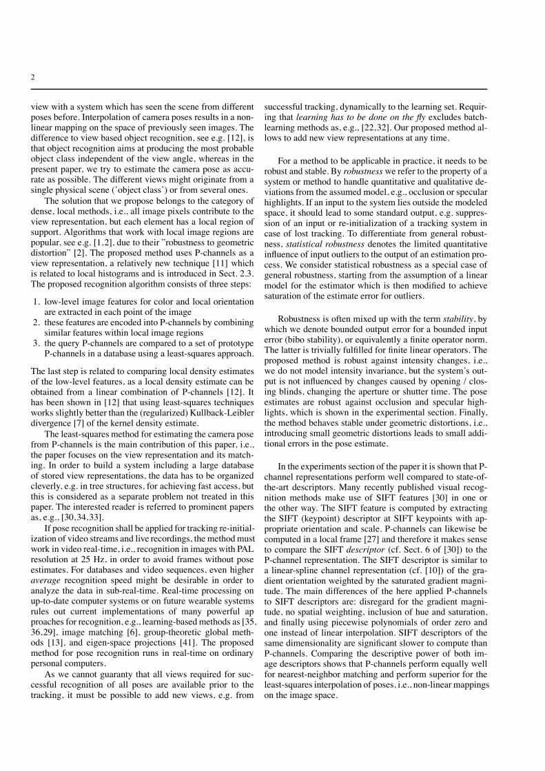
Fig. 2 P-channel representation for the example from Fig. 1. (a) P-channels at original scaling. (b) channels at integer positions. (c) mean valuesof P-channel value vectors.

K components which store the offset from the channel cen-ter. As a consequence, the components of the channel vectorbecome vector-valued (boldface letters) and are denoted aschannel value vectors. The channel vector becomes an arrayof channel value vectors, in other words: a matrix (boldfacecapital).

A set of 1D measurements { f j} j is encoded into P-chan-nels as follows. Without loss of generality the channels arelocated at integer positions (see Fig. 2 (b)). The values f j areaccounted respectively to the channels with the center [ f j],where [ f j] is the closest integer to f j:

pi =1J

J

∑j=1, [ f j ]=i

"

f j! [ f j]1

#

. (8)

Hence, the second component of the channel value vectoris an ordinary histogram estimate of the average number ofoccurrences within the channel bounds over the whole setof measurements. The first component of the channel valuevector contains the average linear offset from the channelcenter over the whole set.

Let f j be a K-dimensional feature vector. The P-channelrepresentation of a set of vectors {f j} j is defined as

pi =1J

J

∑j=1, [f j ]=i

"

f j! [f j]1

#

, (9)

where i is a multi-index, i.e., a vector of indices (i1, . . . , iK)T ,and [f] is defined component-wise as ([ f1], . . . , [ fK])T . Thealgorithmic equivalent to (9) is summarized in Alg. 1. Anexample for the P-channel representation is given in Fig. 2(c).

The main advantage of P-channels opposed to overlap-ping channels is the linear increase of time and space com-plexity with growing number of measurement dimensionsK. Whereas each input sample affects aK channels if the

Algorithm 1 P-channel encoding algorithm.Require: f is scaled correctly for integer channel centers1: for all j do2: for k = 1 to K do3: ik # round( f j,k)4: ok # f j,k! ik5: end for6: l# linear index(i)7: for k = 1 to K do8: pl,k # pl,k +ok9: end for

10: pl,K+1 # pl,K+1 +111: end for

channels overlap with a neighbors, it affects only K+ 1 P-channels. Hence, P-channel representations have a tendencyto be extremely sparse, i.e., only very few values are non-zero. In our implementation we exploit the sparseness bystoring only non-zero values together with their index. Thisresults in a significant speed-up of the channel value deter-mination as well as the further processing.

3 Pose Estimation Based on P-Channels Matching

This section explains the details of the applied technique forpose estimation based on P-channels. We define the featurespace for which the P-channel representations are computed,we define the learning problem for the mapping from mea-sured features to pose vectors, and we apply P-channels andSIFT descriptors to solve this learning problem.

3.1 Feature Space

The image features that we will use for the further process-ing in the P-channel framework are the same as introduced

6

by Felsberg and Hedborg for the purpose of object recogni-tion [12]. The feature space is chosen in an ad-hoc man-ner. The choice is motivated by including color informa-tion, commonly available fast implementation6, robustnessagainst intensity variations, inclusion of geometric informa-tion, and stability against geometric distortions.

The first three points motivate the use of hue h and sat-uration s instead of RGB channels or some advanced colormodel. The value component v is not included in the fea-ture vector, as absolute intensity is not relevant for the reg-istration. Instead, we use it to compute a simple measure ofgeometric information. Stability under geometric distortionsis trivially fulfilled by a finite linear operator (cf. Sect.1).Therefore, we use an ordinary gradient estimate to determinethe local orientation in double-angle representation, cf. [21]:

θ = arg((∂xv+ i∂yv)2) . (10)

The feature vector is complemented with explicit spa-tial coordinates, such that the final vector to be encodedis five-dimensional: hue, saturation, orientation, x-, and y-coordinate. For each image point, such a vector is encodedinto P-channels, where we used up to 8 channels per dimen-sion. Note in this context that periodic entities (e.g. orienta-tion) can be encoded in exactly the same way as linear ones(e.g. x-coordinate).

3.2 Least-Squares Learning of Pose Estimation

Let d be an l-dimensional image descriptor and c an n-dimen-sional camera pose vector. The actual choice for the descrip-tor and the pose representation is not relevant in this sectionand concrete examples will be given in Sect. 3.3. We formu-late our pose estimation problem as follows: By supervisedlearning we want to find the optimal mapping from d to c,represented by the n$ l matrixM:

c=Md . (11)

Note that this equation is related to a linear mapping of den-sity estimates if the latter can be expressed as a linear func-tion of d, which is the case if d is a P-channel represen-tation. The explicit formula for converting P-channels intolinear spline density estimates is given in [12]. Optimalityis defined in terms of least-squares, mostly due to practicalconsiderations. For least-squares efficient solutions applyingthe SVD (singular value decomposition) are available.

For the supervised learning, a set of inputs and outputsof the mapping are given: m pairs of vectors (d j, c j), j =1, . . . ,m. The training set is rewritten as D = [d1 . . .dm] %Rl$m and C = [c1 . . .cm] % Rn$m. In our learning problem,the number of degrees of freedom (unknowns) in the map-ping is by orders larger than number of learning pairs (con-straint equations). We hence obtain an underdetermined sys-

6 We based our implementation on the OpenCV library http://sourceforge.net/projects/opencvlibrary/.

tem of equations. For solving the system, we apply a mini-mum norm approach to our optimization problem:

M= arg minM%S

&M&2F , S = {M % R

n$l ;MD=C} , (12)

where & · &F denotes the Frobenius norm. Minimizing theFrobenius norm ofM guarantees stability by giving an upperbound for the energy of the output [17]. The unique solutionis obtained as (see e.g. introduction to [9], using an additiontranspose operation)

M= CD†, (13)

where D† % Rm$l is the pseudo-inverse of D. For numericalreasons, it is favorable to compute the pseudo inverse by theSVD of D= UΣΣΣVT [31]:

D† = VΣΣΣ †UT . (14)

The pseudo-inverse of ΣΣΣ = diag(σ1, . . . ,σr,0, . . . ,0) reads

ΣΣΣ† = diag(σ!11 , . . . ,σ!1

r ,0, . . . ,0) , (15)

where r ' m is the rank of D.Note that weighting the respective dimensions of c j differ-ently does not affect the result. This can be seen by replac-ing C( = diag(w1, . . . ,wn)C and M( = diag(w1, . . . ,wn)Massuming ∏m

k=1wk )= 0.In operation mode, the mapping is applied to query de-

scriptors, i.e., for a given descriptor dq we search for the cor-responding camera pose cq. The solution is given in terms ofthe pseudo inverse computed above:

cq =Mdq =CD†dq . (16)

Note that due to associativity we can split the RHS into twoparts: The second one,D†dq, which is only depending on theselection of descriptors, samples, and the query, results in anindex function. This index function indicates the similarityof the query view and the respective sample views and canbe used for matching, c.f. [12]. It is independent of the out-put space, i.e., the pose vector, but the matching scores canbe used for interpolation in an arbitrary output matrix / posematrix C. The latter is the first part of the RHS and its pur-pose is to map views to poses. Multiplying the scores fromthe right part with C results in a linear superposition of posevectors for the different views.

In [12], it has been shown that the index function definedabove results in slightly better ROC (receiver operating char-acteristic) curves for pose-invariant object recognition, i.e.,better recognition rates, than the criterion based on an ap-proximation of the Kullback-Leibler divergence. One expla-nation for the better performance of (16) is the higher num-ber of degrees of freedom in the P-channel vector comparedto the converted P-channel vector used in the KLD.

In the same reference, it was proposed not to use theSVD since it cannot be used for live update of learning prob-lems, i.e., it has to be recomputed for every newly added

7

input-output sample. According to [5] it is actually possi-ble to compute the SVD incrementally, and thus, the advan-tages of linear superposition and better performance can becombined with incremental learning. All experiments belowwere however based on the ordinary (batch) SVD.

3.3 Pose Estimation by P-Channels and SIFT Descriptors

In order to obtain a proper pose-estimation algorithm from(16), the pose vector space and the image descriptor haveto be established. Under the assumption of mild variationsof the camera pose, the actual representation of the pose isnot crucial and we chose a non-redundant representation ofthe tangent plane in terms of euclidean position vector and arotation vector:c= [p1 p2 p3 r1 r2 r3]

T. (17)

Note that for scenarios with large variations of the pose an-gle and the camera position, the proper topology of the posespace have to be taken into account and robust representa-tions have to be used. Channel representations of the camerapose seem to be a good choice for achieving this [22].

On the image descriptor side, i.e., for the d-vector, wepropose two solutions: the first one based on P-channels andthe second one, for reference, based on SIFT descriptors.

For the first alternative, we encode the image featureschosen in Sect. 3.1 with four channels for h, s, and θ , re-spectively, and eight channels for both spatial coordinates.This results in 24.576 components per view. The channelvectors are then combined in the matrix D.

For the second alternative, we process each RGB chan-nel separately, as SIFT descriptors are defined for gray-scaleimages. In our experiments this resulted in a significant im-provement compared to first converting the image to gray-scales and also to using other color models, as e.g. YCbCr.We extract the standard descriptors of length 128 at 64 regu-larly spaced positions in the image. This results in the samenumber of components as the P-channel representation andalso assures repeatability. The latter was lost extracting SIFTfeatures at SIFT points, as the order of descriptors becomespermutated. Even with additional SIFT matching step (im-plementation from [43]), the estimates with regularly spacedSIFT descriptors was always preferable to the one with de-scriptors at SIFT points.

Therefore, we are using the SIFT descriptors and notthe complete SIFT features in this comparison, as alreadypointed out in Sect. 1. SIFT features are mostly applied insparse feature matching for estimating epipolar geometry orfinding 2D-3D correspondences, whereas the here consid-ered problem is a model-free 2D-2D matching approach.Hence, the results below should not be interpreted as P-channels being superior to SIFT features, but as P-channelsperforming equally well as or superior to SIFT descriptorswhen it comes to 2D-2D matching and interpolation. Theimplementation for the SIFT descriptor extraction is takenfrom [43], as the original implementation does not exist forall platforms.

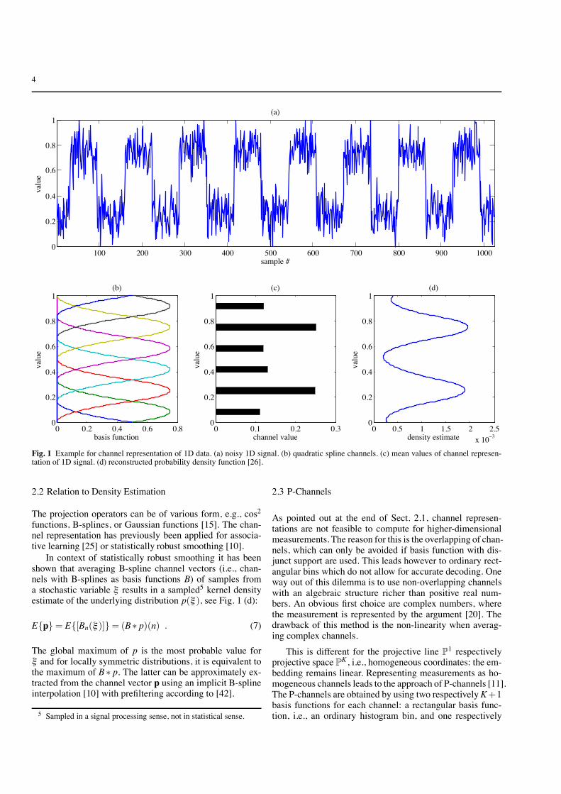
Fig. 3 Top: perspective view on the synthetic scene (40 cm deep, 50cm wide, and 25 cm high). Bottom: example for synthetic fisheye im-age with noise.

4 Recognition Experiments

In this section we present two experiments, one quantita-tive using synthetic images from a fisheye camera, and onequalitative experiment with images from a real fisheye cam-era. As pointed out above, the proposed method is a 2D-2Dmatching method and therefore we compare our method toa SIFT descriptor based 2D-2D matching method. We makeno efforts to compare our method to model-based 2D-3Dpose estimation method, since those solve a different prob-lem, where a model of the scene is available.

4.1 Pose Estimation Experiment with Synthetic Data

As it is difficult to acquire test data with noise-free pose vec-tors from a real fisheye camera, the quantitative experimenthas been done on synthetic data with known pose angles. Weexcluded noisy pose vectors, as the primary focus is on therobust processing of scene views, and not on the regressionof pose vectors. The latter task can be accomplished withstate of the art methods from control theory [23].

The virtual scene and one instance of the generated syn-thetic views are depicted in Fig. 3. The images were ren-dered (linear in angle, 180* field of view) and noise (Gaus-sian noise with 10% standard deviation of the intensity range[0. . . 255]) was added afterwards. The virtual camera was al-ways located inside the scene area somewhere over the ”Vi-

8

Table 1 Estimation errors for the different tested methods.

method position RMSE [cm] rotation error [*]

SIFT/D 0.51 1.1SIFT/C 1.37 4.3Channel/D 0.52 1.1Channel/C 0.21 0.3

talis” package in Fig. 3, pointing roughly downwards. Thedepth range was thus about 8 cm to about 30 cm.

The views for training were selected by picking all viewswhere the pose vector either has a local extremum or an in-flection point. Altogether, we considered 252 views and se-lected 72 for training. Note that the minimum number ofviews to span a six-dimensional space is 26 = 64, i.e., wehave only selected eight redundant views by the method de-scribed above. Choosing views by a different scheme, leadsto a slight degradation of results. For practical applications,we recommend to use at least the extrema. If too few ex-trema are available (less than 64, as it is the case here), onecan choose further views pretty arbitrarily, unless they aretoo close to the already existing views.

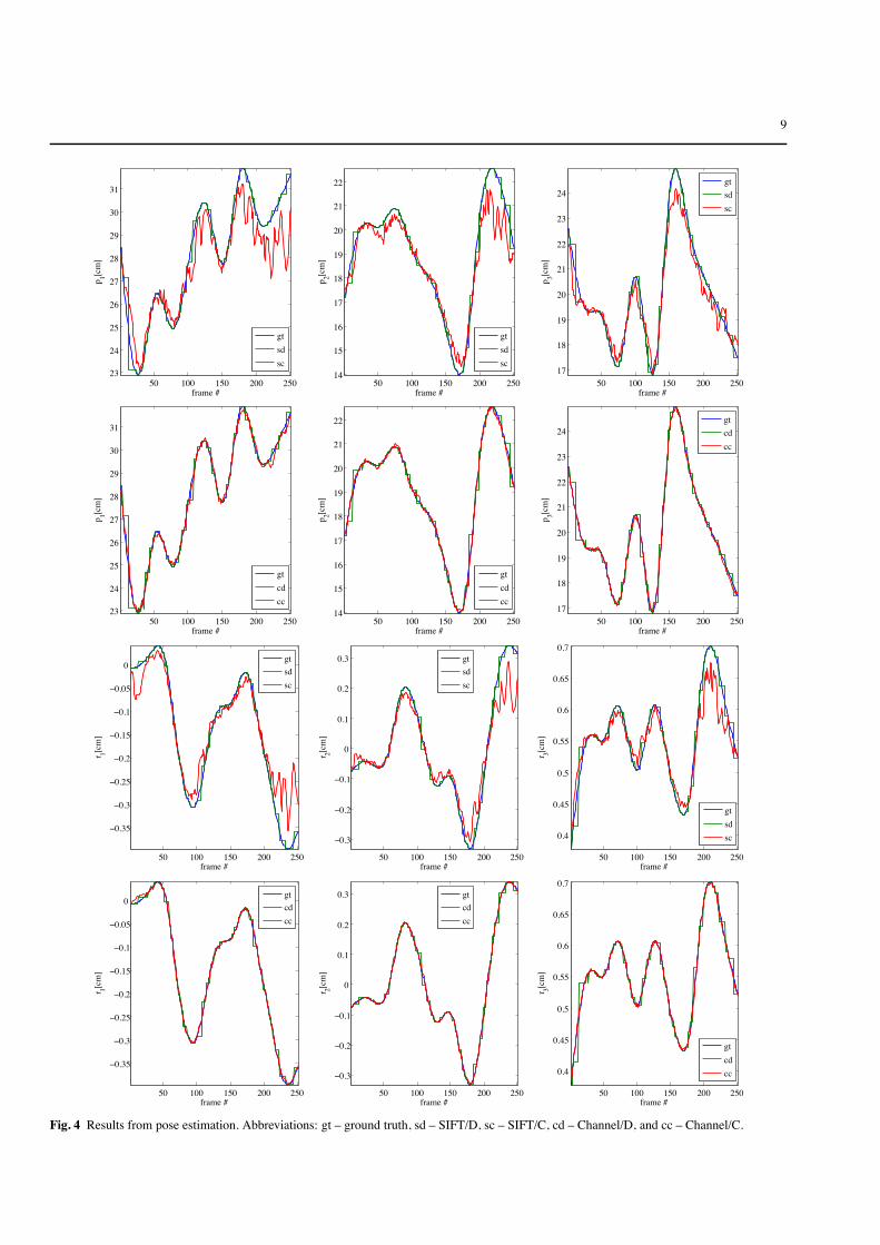
The results are summarized in Fig. 4, displaying the es-timates of all six pose vector components for four differentmethods. Tab. 1 lists the errors separately for the positionpart (root mean square error) and rotation part (angular erroraccording to [28]) of the pose vector. The first position co-ordinate corresponds to the horizontal position in Fig. 3, thesecond to the vertical position, and the third to the depth po-sition. The methods considered were: SIFT descriptor basednearest-neighbor estimate (SIFT/D), SIFT based continuousinterpolation (SIFT/C), channel based nearest-neighbor es-timate (Channel/D), and channel based continuous interpo-lation (Channel/C). Here, continuous interpolation refers tothe superposition according to (16) and nearest-neighbor es-timate refers to

cq = c j0 where j0 = argmaxj

(D†dq) j . (18)

From the numerical results in Tab. 1 it is evident that forthe nearest-neighbor case, SIFT and channel based descrip-tors do not significantly differ. For the case of interpolation,the SIFT based method becomes worse by factor three tofour, whereas the channel based method improves by fac-tor three to four. This can be explained by considering thegraphs in Fig. 4.

When looking at the different results from linear super-position of the pose vectors, the SIFT based interpolation hasa tendency to flatten extrema and to introduce oscillationsinstead. This is a typical sign of over-fitting with alternatingsigns, which often results from non-compact basis functions.Linear superposition of P-channels, however, corresponds toa superposition of local linear models, thus avoiding oscil-lations by locality. The oscillations are the main reason whyperformance degrades for SIFT descriptors, but improves forchannel representations.

Fig. 5 Example for real fisheye image.

4.2 Scene Recognition Experiment with Real Data

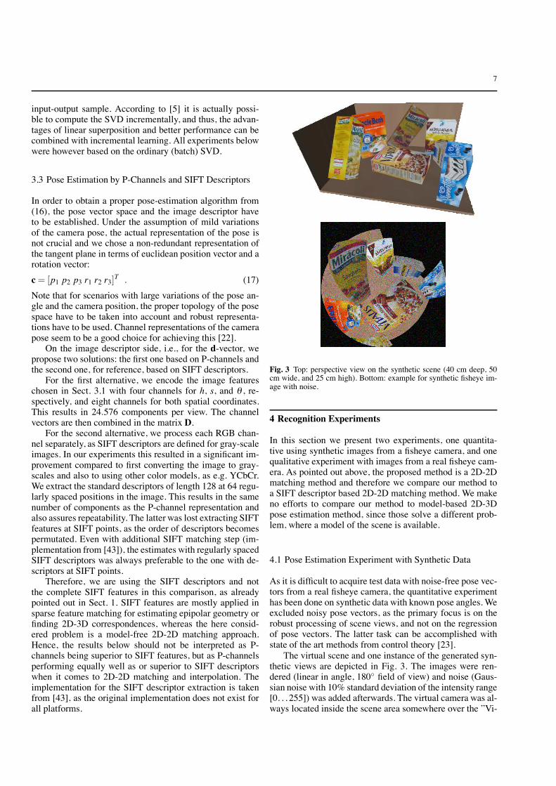
The task considered in this experiment is to find, for a givenview, the stored view from a catalogue of views which ismost similar to the given input view. In this case, the viewswere obtained with a fisheye lens. As we use real data with-out known pose angles, see Fig. 5 for an example, the evalu-ation had to be done manually, based on subjective criteria.This is done in the following way.

In the training, a number of views is selected by a strat-egy based on visual dissimilarity instead of extremal posevectors or inflections points. We initialize the recognitionsystem with P-channel representations of two different views,i.e., the initial matrix D is of size l$2. For all vectors fromthe training set {d j} j , it is now checked whether the indexfunction that responds best delivers a matching score abovea certain threshold:

minj

maxi

(D†d j)i > θ , (19)

where θ is empirically chosen as 0.48 in order to give a rea-sonable number of columns in the final D. If and only if (19)is not fulfilled, the vector d j with the worst match is addedto D, and (19) is re-evaluated.

In operation mode, the views represented in D are dis-played together with a query view and the best match is in-dicated, see Fig. 6. If and only if the best match is inspectedto be the correct view, the recognition task is considered suc-cessful.

In our experiment with 167 views, divided into 38 trainedviews and 129 test views, only two views are not correctlymatched. In both cases this happens due to missing fittingviews inD, and a better fitting view is scored second. Match-ing scores are low in both cases.

Interestingly, no views have been selected forD that con-tain the person visible in the query view in Fig. 6. The cor-rectness of the matching is not influenced by the partial oc-clusion caused by the person who appeared in seven views.The matching was not distorted by specular highlights or

9

50 100 150 200 25023

24

25

26

27

28

29

30

31

frame #

p 1[cm

]

50 100 150 200 25014

15

16

17

18

19

20

21

22

frame #

p 2[cm

]

50 100 150 200 25017

18

19

20

21

22

23

24

frame #

p 3[cm

]

gtsdsc

gtsdsc

gtsdsc

50 100 150 200 25023

24

25

26

27

28

29

30

31

frame #

p 1[cm

]

50 100 150 200 25014

15

16

17

18

19

20

21

22

frame #

p 2[cm

]

50 100 150 200 25017

18

19

20

21

22

23

24

frame #

p 3[cm

]

gtcdcc

gtcdcc

gtcdcc

50 100 150 200 250

−0.35

−0.3

−0.25

−0.2

−0.15

−0.1

−0.05

0

frame #

r 1[cm

]

50 100 150 200 250

−0.3

−0.2

−0.1

0

0.1

0.2

0.3

frame #

r 2[cm

]

50 100 150 200 250

0.4

0.45

0.5

0.55

0.6

0.65

0.7

frame #

r 3[cm

]

gtsdsc

gtsdsc

gtsdsc

50 100 150 200 250

−0.35

−0.3

−0.25

−0.2

−0.15

−0.1

−0.05

0

frame #

r 1[cm

]

50 100 150 200 250

−0.3

−0.2

−0.1

0

0.1

0.2

0.3

frame #

r 2[cm

]

50 100 150 200 250

0.4

0.45

0.5

0.55

0.6

0.65

0.7

frame #

r 3[cm

]

gtcdcc

gtcdcc

gtcdcc

Fig. 4 Results from pose estimation. Abbreviations: gt – ground truth, sd – SIFT/D, sc – SIFT/C, cd – Channel/D, and cc – Channel/C.

10

0: 3

13: 6

22: 3

29: 2

35: 0

39: 0

41: 5

45: 2

55: 0

59: 1

2

65: 1

67: 2

72: 1

78: 0

83: 0

88: 3

93: 2

97: 1

4

108:

0

110:

2

111:

0

114:

0

115:

6

116:

0

117:

0

120:

3

122:

4

123:

0

127:

1

128:

0

130:

0

131:

0

133:

0

134:

8

139:

4

146:

5

151:

0

166:

84

161

Fig. 6 Window displaying all views represented by D, one query view (lower right), and the best match indicated in red. The first number at eachview indicates the index in the data set. The second number indicates the matching score in %. As it can be seen in this example, the matchingis robust to partial occlusion of the scene.

other distortions as comatic and chromatic aberration, or ver-tical smear (CCD artifact caused by local over-exposure, oc-curred in 42 instances). The robustness against occlusionand lighting distortions is a particularly important propertyin context of markerless tracking systems, since the systemis initialized, i.e., trained, in front of an empty scene that islater partially occluded by various objects and exposed toother lighting conditions.

Performing the same experiment using SIFT descriptorswas somehow problematic, since using a fixed threshold in(19) resulted in much more training views due to a veryslowly increasing minimum score. The minimum score de-creases in the beginning and it takes more than 38 viewsbefore the minimum score is larger than the initial minimumscore. Instead, we fixed the number of views to 38, whichhowever leads to lower matching scores in general.

The matching works similar well as the one based onP-channels. Three non-correct matches were found, but thisis a non-significant difference for a test set of 129 instances.The matching scores were however less distinct, i.e., it is notpossible to predict false matches from the matching score.The SIFT-based method showed the same robustness againstocclusion and image distortions as our proposed method.

Overall, the two methods perform much more similarly onthe real data than in the synthetic interpolation experiment.This was however expected as no interpolation could be testedon the real data.

4.3 Efficient Implementation

So far we have shown that P-channel based pose estimationworks reasonable well, in particular it works better for in-terpolation than the SIFT-based method. What remains toshow is that P-channel encoding can be achieved in videoreal-time.

First of all, P-channel encoding is fast because only oneloop through the image is required [11], see also Alg. 1. Foreach image point, each image feature hue, saturation, orien-tation, and position, i.e., five dimensions altogether, is addedto the appropriate set of bins. Under appropriate scaling ofthe feature vector, the multi-index of the bins is computedby rounding the feature vector to the next integer in eachcomponent. The five non-integer parts define the respectiveoffsets and the sixth component of the P-channel is increasedby one.

11

After computing the image features only 24 operationsper image pixel are required for the encoding. For PAL res-olution (720 by 576, 25Hz), this results in less than 250 mil-lion operations per second. The initial feature extraction7 re-quires about 32 operations per pixel, including the rescaling.Hence, less than 600 million operations are required for thecomplete P-channel extraction, and thus, real time perfor-mance is realistic on current systems (2.4GHz dual core),even if adding overhead for memory accesses, operative sys-tem, etc. This is significantly faster than the extraction ofSIFT descriptors, which has also been verified in the imple-mentation (SIFT implementation [43]).

For the matching of descriptors, the computational costsare given by the matrix multiplication (16), i.e., 2 · l · n op-erations are required, which is neglectable compared to theP-channel encoding if the average number of channel per di-mension is below twelve. In the described experiments thenumber of required operations for the matching was below10 million per second. If the number of channels increasessignificantly, the P-channels must be implemented as sparsematrices. This limits the effort independent of the number ofchannels, as an upper bound is obtained that is linear withthe number of pixels [11].

Measurements of our C++ implementation confirmed thetheoretic considerations above. Without tweaking and spe-cial programming (e.g. GPU, using dual core, MMX, etc.),the whole scene registration process takes 0.039 seconds perPAL image, i.e., full framerate at full resolution. This cor-responds roughly to about 600 million operations which isreasonable since many operations need more than one clockcycle and some type conversions are required. The main bot-tleneck of the implementation is the atan2 in (10), whichoriginally took 0.043 seconds (including the necessary typeconversions) and which has been replaced by a look-up tableto achieve full framerate.

5 Conclusion

We have presented a novel approach to pose recognition andinterpolation suitable for real-time applications. The methodis based on a sampled kernel density estimate, computedfrom the P-channel representation of the considered imagefeatures. The density estimates from the test set are classi-fied using a least-squares learning technique implementedusing the SVD. It has been shown in two experiments withfisheye data that– the method performs equally well as SIFT descriptor

based recognition for finding the closest view despite itsreal-time capability,

– the method outperforms SIFT descriptor if the pose an-gle is interpolated using the matching function (SVD),

– the method is robust against occlusion, changes of light-ing conditions, and common distortions.

7 Note that the feature extraction needs to be done on the wholeimage in general, as the localization of relevant areas is unknown atthis stage.

This makes the method a suitable tool for the initializationof pose tracking in the MATRIS system and similar applica-tions as, e.g., visual navigation.

Acknowledgements We thank our project partners for providing thetest data used in the experiments. We thank in particular Graham Thomas,Jigna Chandaria, Gabriele Bleser, Reinhard Koch, and Kevin Koeser.

References

1. S. Agarwal, A. Awan, and D. Roth. Learning to detect objects inimages via sparse, part-based representation. IEEE Transactionson Pattern Analysis and Machine Intelligence, 26(11):1475–1490,2004.

2. A. Berg, T. Berg, and J. Malik. Shape matching and object recog-nition using low distortion correspondence. In IEEE ComputerVision and Pattern Recognition, 2005.

3. C. M. Bishop. Neural Networks for Pattern Recognition. OxfordUniversity Press, New York, 1995.

4. C. M. Bishop. Pattern Recognition and Machine Learning.Springer, 2006.

5. M. Brand. Incremental singular value decomposition of uncer-tain data with missing values. Technical Report TR-2002-24, Mit-subishi Electric Research Laboratory, May 2002.

6. Q. Chen, M. Defrise, and F. Deconinck. Symmetric phase-onlymatched filtering of Fourier-Mellin transforms for image registra-tion and recognition. Transactions on Pattern Analysis and Ma-chine Intelligence, 16(12):1156–1168, December 1994.

7. T. M. Cover and J. A. Thomas. Elements of Information Theory.Wiley, New York, 1991.

8. E. Dimitriadou, A. Weingessel, and K. Hornik. Fuzzy voting inclustering. In Fuzzy-Neuro Systems, pages 63–75, 1999.

9. G. Farneback. Spatial domain methods for orientation and ve-locity estimation. Lic. Thesis LiU-Tek-Lic-1999:13, Dept. EE,Linkoping University, March 1999.

10. M. Felsberg, P.-E. Forssen, and H. Scharr. Channel smoothing: Ef-ficient robust smoothing of low-level signal features. IEEE Trans-actions on Pattern Analysis and Machine Intelligence, 28(2):209–222, 2006.

11. M. Felsberg and G. Granlund. P-channels: Robust multivariatem-estimation of large datasets. In International Conference onPattern Recognition, Hong Kong, August 2006.

12. M. Felsberg and J. Hedborg. Real-time visual recognition of objects and scenes using p-channel matching. In Proc. 15th Scan-dinavian Conference on Image Analysis, volume 4522 of LNCS,pages 908–917, 2007.

13. M. Ferraro and T. M. Caelli. Lie transformation groups, inte-gral transforms, and invariant pattern recognition. Spatial Vision,8(4):33–44, 1994.

14. R. B. Fisher, K. Dawson-Howe, A. Fitzgibbon, C. Robertson, andE. Trucco. Dictionary of Computer Vision and Image Processing.Wiley & Sons, 2005.

15. P.-E. Forssen. Low and Medium Level Vision using Channel Rep-resentations. PhD thesis, Linkoping University, Sweden, 2004.

16. M. S. Gazzaniga, R. B. Ivry, and G. R. Mangun. Cognitive Neuro-science, Second Edition. W. W. Norton & Company, March 2002.

17. K. Gopalsamy. Stability of artificial neural networks with im-pulses. Applied Mathematics and Computation, 154(3):783–813,2004.

18. G. H. Granlund. The complexity of vision. Signal Processing,74(1):101–126, April 1999. Invited paper.

19. G. H. Granlund. An Associative Perception-Action Structure Us-ing a Localized Space Variant Information Representation. InProceedings of Algebraic Frames for the Perception-Action Cycle(AFPAC), Kiel, Germany, September 2000.

20. G. H. Granlund. Personal communication, 2006.21. G. H. Granlund and H. Knutsson. Signal Processing for Computer

Vision. Kluwer Academic Publishers, Dordrecht, 1995.

12

22. G. H. Granlund and A. Moe. Unrestricted recognition of 3-d ob-jects for robotics using multi-level triplet invariants. Artificial In-telligence Magazine, To appear 2004.

23. F. Gustafsson. Adaptive filtering and change detection. John Wi-ley & Sons, Ltd., 2000.

24. J. Hol, T. B. Schon, H. Luinge, P. Slycke, and F. Gustafsson. En-abling real-time tracking by fusing measurements from inertialand vision sensors. submitted to the same issue, 2007.

25. B. Johansson, T. Elfving, V. Kozlov, Y. Censor, P.-E. Forssen, andG. Granlund. The application of an oblique-projected landwe-ber method to a model of supervised learning. Mathematical andComputer Modelling, 43:892–909, 2006.

26. E. Jonsson and M. Felsberg. Reconstruction of probability densityfunctions from channel representations. In Proc. 14th Scandina-vian Conference on Image Analysis, 2005.

27. E. Jonsson and M. Felsberg. Accurate interpolation in appearance-based pose estimation. In Proc. 15th Scandinavian Conference onImage Analysis, volume 4522 of LNCS, pages 1–10, 2007.

28. H. Knutsson and M. Andersson. Robust N-dimensional orien-tation estimation using quadrature filters and tensor whitening.In Proceedings of IEEE International Conference on Acoustics,Speech, & Signal Processing, Adelaide, Australia, April 1994.IEEE.

29. N. Kruger. Learning object representations using a priori con-straints within ORASSYLL. Neural Computation, 13(2):389–410, 2001.

30. D. G. Lowe. Distinctive image features from scale-invariant key-points. International Journal of Computer Vision, 60(2):91–110,2004.

31. M. Muhlich and R. Mester. A considerable improvement in non-iterative homography estimation using TLS and equilibration. Pat-tern Recognition Letters, 22:1181–1189, 2001.

32. E. Murphy-Chutorian, S. Aboutalib, and J. Triesch. Analysis ofa biologically-inspired system for real-time object recognition.Cognitive Science Online, 3:1–14, 2005.

33. D. Nister and H. Stewenius. Scalable recognition with a vocab-ulary tree. In IEEE Computer Vision and Pattern Recognition,2006.

34. S. Obdrzalek and J. Matas. Sub-linear indexing for large scaleobject recognition. In W. F. Clocksin, A. W. Fitzgibbon, andP. H. S. Torr, editors, BMVC 2005: Proceedings of the 16th BritishMachine Vision Conference, volume 1, pages 1–10, London, UK,September 2005. BMVA.

35. M. Pontil and A. Verri. Support vector machines for 3d objectrecognition. IEEE Transactions on Pattern Analysis and MachineIntelligence, 20(6):637–646, 1998.

36. D. Roobaert, M. Zillich, and J.-O. Eklundh. A pure learning ap-proach to background-invariant object recognition using pedagog-ical support vector learning. In IEEE Computer Vision and PatternRecognition, volume 2, pages 351–357, 2001.

37. J. Skoglund and M. Felsberg. Evaluation of subpixel tracking al-gorithms. In International Symposium on Visual Computing, vol-ume 4292 of LNCS, pages 374–382, 2006.

38. J. Skoglund and M. Felsberg. Covariance estimation for sad blockmatching. In Proc. 15th Scandinavian Conference on Image Anal-ysis, volume 4522 of LNCS, pages 372–382, 2007.

39. H. P. Snippe and J. J. Koenderink. Discrimination thresholdsfor channel-coded systems. Biological Cybernetics, 66:543–551,1992.

40. D. Stricker, G. Thomas, and J. Chandaria. The matris project: real-time markerless camera tracking for ar and broadcast applications.submitted to the same issue, 2007.

41. M. Turk and A. Pentland. Eigenfaces for recognition. Journal ofCognitive Neuroscience, 3(1):71–86, 1991.

42. M. Unser. Splines – a perfect fit for signal and image processing.IEEE Signal Processing Magazine, 16:22–38, November 1999.

43. A. Vedaldi. An open implementation of SIFT. http://vision.ucla.edu/+vedaldi/code/sift/sift.html, last accessed23/05/2007, 2007.