real-time moving obstacle detection using optical ﬂow models

Real-time moving obstacle detection using optical

flow models

Christophe Braillon1, Cedric Pradalier2, James L. Crowley1 and Christian Laugier1

1Laboratoire GRAVIR 2CSIRO ICT Centre

INRIA Rhone-Alpes Autonomous Sytems Lab

655 avenue de l’Europe 1 Technology court

38334 Saint Ismier Cedex, France Pullenvale QLD 4069, Australia

Email: [email protected] Email: [email protected]

Abstract— In this paper, we propose a real-time method todetect obstacles using theoretical models of optical flow fields.The idea of our approach is to segment the image in two layers:the pixels which match our optical flow model and those that donot (i.e. the obstacles). In this paper, we focus our approach ona model of the motion of the ground plane. Regions of the visualfield that violate this model indicate potential obstacles.

In the first part of this paper, we will describe the method weused to determine our model of the ground plane’s motion. Thenwe will focus on the method to match both the model and thereal optical flow field.

Experiments have been carried on the Cycab mobile robot inreal-time on a standard PC laptop.

I. INTRODUCTION

This work takes place in the general context of mobile

robots navigating in open and dynamic environments. Com-

puter vision for ITS (Intelligent Transport Systems) is an active

research area [1]. One of the key issues of ITS is the ability

to avoid obstacles. This requires a method to perceive them.

In this article we address the problem of obstacle sensing

through their motion (optical flow) in an image sequence. The

perceived motion can be caused either by the obstacle itself

or by the motion of the camera (which is the motion of the

robot in the case of a camera fixed on it).

Many methods have been developed to find moving objects

in an image sequence. Most of them use a fixed camera and

use background subtraction (for example in [2] and [3]).

Others, based on optical flow have been inspired by

biomimetic models [4]. For example, Franceschini and his

collaborators have demonstrated models of optical flow based

on insect retinas and have shown how such models may be

used for local navigation. Duchon [5] proposed a reactive

obstacle avoidance method based on insects’ behaviour, and

more recently Muratet and al. [6] implemented a model of the

visual system of a fly, using a model helicopter. A survey of

similar investigations is provided by Lee et al. ( [7], as well as

[8], [9]), who studied human perception of optical flow and

their related behaviours. Other new approches by Hrabar et

al. ( [10], [11]) are based on optical flow and stereo camera

to navigate urban environments with UAVs (Unmanned Aerial

Vehicles) in a reactive way by doing a control oriented fusion.

These investigations cannot be easily integrated in complex

systems, because they are purely reactive and do not provide

the high level of information required for modern navigation

techniques in unstructured environments.

Recently, in [12], a new approach to obstacle avoidance has

been developed, based on ground detection by finding planes

in images. The weak point of this method is that the robot

must be in a static environment.

Model based approches using egomotion have been demon-

strated in [13], [14]. The first one detects the ground plane

by virtually rotating the camera and visually estimating the

egomotion. The second one uses dense stereo and optical

flow to find moving objects and robot ego-motion. These two

methods have a large computational cost as several successive

calculations (stereo, optical flow, egomotion, ...) are required.

In this paper, we demonstrate that by knowing the motion of

the camera (in our case we used the odometric information),

we can model the motion of the ground plane and determine

the location of the obstacles.

In a first step we determine the ground plane’s optical flow

field using the odometric data. In the next step, we try to match

this theoretical field with the actual motion field. The pixels

which do not match the model are either obstacles (objects

outside the ground plane) or objects in the ground plane that

are moving.

One key point in this method is that we do not compute

explicitly the optical flow of the image at any time. Optical

flow computation is very expensive in terms of CPU time,

is inaccurate and sensitive to noise. In general we can see

in the survey led by Barron et al. ( [15]) that the accuracy

of optical flow computation is linked to the computational

cost. We model the expected optical flow (which is easy and

quick to compute) to get rid of the inherent noise and the time

consuming optical flow step. As a consequence we are able to

demonstrate robust and real-time obstacle detection.

II. OUR OPTICAL FLOW MODEL

By definition, an optical flow field is a vector field that

describes the velocity of pixels in an image sequence. The

Intelligent Vehicles Symposium 2006, June 13-15, 2006, Tokyo, Japan

466

13-6

first step of our method is the modeling of the optical flow

field for our camera.

This model is based on the classical pinhole camera model,

that is to say, we neglect the distortion due to the lens. We

also assume that there is no skew factor. We will see in the

experimental results that these two assumptions are valid.

A. Notations

Figure 1 shows the position of the camera fixed on our

Cycab robot, the coordinates frames and the notations we will

use in all this paper.

The robot’s position is given in the coordinate system of

the world by (x, y) and its orientation is called θ. In the next

parts we will call x, y, θ the three derivatives of x, y, θ with

respect to time.

We assume that at time t, we know the intensity image It,

the linear velocity vt and rotational velocity ωt of the robot.

Fig. 1. Configuration of the camera on our mobile robot. The red linerepresents the abscissa axis and the green one the ordinate axis. The originof the robot frame is the projection of the middle of the rear axis on theground. We call (cx, cy , cz) the position of the camera in this frame and φ

its orientation (we suppose that only the tilt is not null).

We use the projective geometry formalisms to simplify the

theoretical aspects of the motion modeling. The points of the

world are noted (X, Y, Z, 1)T in the world frame and the pixel

coordinates are (u, v, w)T .

The camera’s projection matrix (pinhole model) with refer-

ence to the camera frame is written:

PCamera =

αu 0 u0 0

0 αv v0 0

0 0 1 0

B. Description of the model

The model we propose to study is the one of the ground.

We assume that the ground is a plane located at Z = 0 coor-

dinate. This means that the ground plane’s points are written

(X, Y, 0, 1)T Thus we can write the projection equation of the

ground point on the image as:

u

v

w

Image

= PWorld

X

Y

0

1

World

(1)

In our case, we have a projection from one plane (the

ground) to another (the image), which can be expressed as

an homography:

u

v

w

Image

= H

X

Y

1

Ground

(2)

Actually, the matrix H is the matrix P in which we remove

the third column. This point is important because we need an

analytical expression of H which involves the position and

orientation of the robot and camera.

The homography matrix allows us to estimate the position

of a ground point in the image, but in this study, we need to

compute the optical flow for a given pixel. Therefore, we need

to differentiate equation (2) so that we can infer the relation

between pixel coordinates and the related optical flow vector.

u

v

w

Image

= H

X

Y

1

Image

+ H

X

Y

0

Image

(3)

Since we are working on the ground pixels, the relation

can be simplified because they are stationary in the world

coordinate system, thus X = 0 and Y = 0. The new relation

is:

u

v

w

Image

= H

X

Y

1

Image

(4)

From equation (2) and (4) we can infer the following

relation between the homogeneous coordinates of a pixel of

the ground and its coordinates derivatives:

u

v

w

Image

= HH−1

u

v

w

Image

(5)

Using equation (5) we can express the optical flow vector~f (u, v, w) by:

~f (u, v, w) =

(

˙( u

w

)

,˙( v

w

)

)

=

(

uw + uw

w2,vw + vw

w2

)


467

As we on know the u and v coordinates of the pixels we

need to simplify the previous equation to be able to compute

the optical flow vectors. We use the following transformations:

(

u′

v′

)

=1

w

(

u

v

)

and

u′

v′

w′

=1

w

u

v

w

and finally, by combining with equation (5), we obtain:

u′

v′

w′

Image

= HH−1

u′

v′

1

Image

(6)

In equation (6) (u′, v′) are the euclidian coordinates of

a pixel in the image (whereas (u, v, w) are its projective

coordinates).

Now we can obtain the optical flow vector ~f for the pixel

(u′, v′) by the formula:

~f(u′, v′

) =

(

u′ − u′w′

v′ − v′w′

)

(7)

Finally from equations (6) and (7) we can express the

theoretical optical flow vector for each pixel in the image (with

the assumption that each pixel is in the ground plane).

C. Evaluation of the homography matrix

As we only focus on a differential problem, we

can assume that the robot has the configuration

(x = 0, y = 0, θ = 0) all the time. In this case, the velocities

are:(

x = vt, y = 0, θ = ωt

)

, where vt and ωt are the linear

and angular velocities of the robot, respectively.

Using the notations introduced in section II-A, we can

express the projection matrix and the homography matrix as

well:

H =

h1,1 h1,2 h1,3

h2,1 h2,2 h2,3

h3,1 h3,2 h3,3

with:

h1,1 = u0 cos φ

h1,2 = −αu

h1,3 = αu + u0 (− cos φ + cz sin φ)

h2,1 = −αu sin φ + v0 cos φ

h2,2 = 0

h2,3 = αv (sin φ + cz cos φ) + v0 (− cos φ + cz sin φ)

h3,1 = cos φ

h3,2 = 0

h3,3 = − cos φ + cz sin φ

We have also:

H =

h1,1 h1,2 h1,3

h2,1 h2,2 h2,3

h3,1 h3,2 h3,3

with:

h1,1 = αuωt

h1,2 = u0ωt cos φ

h1,3 = −u0vt cos φ

h2,1 = 0

h2,2 = (−αv sin φ + v0 cos φ) ωt

h2,3 = (αv sin φ − v0 cos φ) vt

h3,1 = 0

h3,2 = ωt cos φ

h3,3 = −vt cos φ

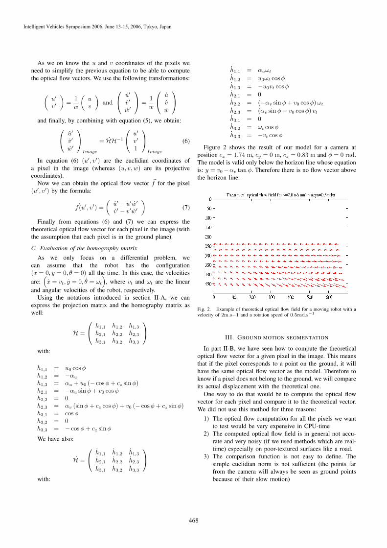
Figure 2 shows the result of our model for a camera at

position cx = 1.74 m, cy = 0 m, cz = 0.83 m and φ = 0 rad.

The model is valid only below the horizon line whose equation

is: y = v0 −αv tanφ. Therefore there is no flow vector above

the horizon line.

Fig. 2. Example of theoretical optical flow field for a moving robot with avelocity of 2m.s−1 and a rotation speed of 0.5rad.s−1

III. GROUND MOTION SEGMENTATION

In part II-B, we have seen how to compute the theoretical

optical flow vector for a given pixel in the image. This means

that if the pixel corresponds to a point on the ground, it will

have the same optical flow vector as the model. Therefore to

know if a pixel does not belong to the ground, we will compare

its actual displacement with the theoretical one.

One way to do that would be to compute the optical flow

vector for each pixel and compare it to the theoretical vector.

We did not use this method for three reasons:

1) The optical flow computation for all the pixels we want

to test would be very expensive in CPU-time

2) The computed optical flow field is in general not accu-

rate and very noisy (if we used methods which are real-

time) especially on poor-textured surfaces like a road.

3) The comparison function is not easy to define. The

simple euclidian norm is not sufficient (the points far

from the camera will always be seen as ground points

because of their slow motion)


468

To solve the problem we use a generative method. For

each pixel we calculate the theoretical optical flow vector

and determine if it is a possible displacement. To do that,

we measure the similarity of a pixel (u′, v′)T

in an image It

with the pixel (u′, v′)T− ∆t ~f (u′, v′) in image It−∆t.

Thus we define a new image Jt of similarity using the

following formula:

Jt(p) = SimIt,It−∆t

(

p, p − ∆t ~f (p)

)

(8)

Where p = (u′, v′)T is a pixel in the image and

SimA,B (p, q) is a similarity between the neighbourhood of

pixel p in image A and the neighbourhood of pixel q in image

B. We will assume that the intensity of the points will not

change between images A and image B. We can see on figure

3 an example of similarity measure between two consecutive

images.

Frame 352 Frame 353

Fig. 3. Similarity measurement: on the top left, image It−∆t, on the topright, image It. On the bottom the result of a similarity measure. The hatchedregion corresponds to the area where the theoretical flow cannot be computed(these pixels will never belong to the ground)

We tried several similarity measures such as: SAD (Sum

of Absolute Differences), SSD (Sum of Squares Differences),

ZSAD (Zero mean Sum of Absolute Differences), ZSSD

(Zero mean Sum of Squared Differences), ZNCC (Zero mean

Normalized Cross Correlation). The best result were given

by the SAD and SSD measures. Actually ZSAD, ZSSD and

ZNCC are zero-mean and ZNCC is normalized, this leads in

general to incorrect associations, because they can associate a

dark region and a bright one. In our case, the lighting condition

between two images are the same, that is why the best results

were given by SAD and SSD. Figure 4 shows the results of

the different similarity measures.

(a) (b)

SAD SSD

ZSSD ZNCC

Fig. 4. Examples of similarity measures between image (a) and (b)

We can see that the SSD measure is more selective than

SAD. This is due to the fact that SSD emphasize big differ-

ences because of the square. As a result, we have more details

in SAD but also more noise. Therefore we will use the SSD

measure in all our experiments.

The SSD image we obtain is normalized by its maximum

value so that the each pixel has a value between 0 and 1. We

have then applied a threshold of 0.7 to segment the obstacles.

IV. EXPERIMENTAL RESULTS

A. System description

In our experiments, we use a Cycab mobile robot, which

provides odometric measurements and a digital video stream

(a color camera is fixed on the front of the robot). We need to

have synchronized odometry data and video stream (otherwise

the detection will be incorrect). The robot is driven manually

in a carpark where pedestrians and cars are moving. To give

an overview of our experimental results, we will use a video

where two pedestrians are crossing in front of the robot.

B. Results and comments

Figures 5 and 6 show the video sequence on which we

superimposed the contour of the detected objects and the SSD

image for the corresponding frames, respectively. The horizon-

tal line in the image corresponds to the horizon. Obviously all

the pixels above this line do not belong to the ground plane.

We can also see that even far objects are detected (for example

on frame 135 on figure 5).


469

We have simulated a CPU overload in our experiments by

running useless processes when doing our experiments. It has

shown that even with gaps in the video sequence (some frames

were lost because of other processes slowing the computer

down) our method is able to detect the obstacles correctly .

This is an important characteristic since the robots’ embedded

computers have a high CPU load (especially when using

computer vision) and frame loss may occur.

Frame 135 Frame 217

Frame 258 Frame 323

Frame 352 Frame 371

Fig. 5. Six frames of the video sequence. The red curves are the contoursof the obstacles (see figure 6).

C. Discussion

We have not led a quantitative survey on the impact of pan

and roll of the camera, its position error and flatness of the

ground, but when watching the video, we can see that the roll

is not null (we can easily see that on figure 7) and it does not

seem to disturb the detection. Furthermore the position of the

camera has been roughly estimated. Thus we can guess that

the impact of such errors is not significant, but we will study

the effect of these parameters in a future work.

The model we described in II considers that the ground

points are not moving which is a reasonable assumption. When

there is a fixed shadow on the ground, no obstacles are detected

and the observed optical flow is the same as the models’. When

the object that casts the shadow starts moving, the optical flow

on the shadows’ edge changes and does not match the model

Frame 135 Frame 217

Frame 258 Frame 323

Frame 352 Frame 371

Fig. 6. SSD images corresponding to figure 5. The grey scale correspondsto the SSD value. White means that the SSD is low and black that it is high.The hatched part corresponds to an area of the image which cannot be theground (the algorithm mark these pixel as unusable)

anymore. Therefore in our experiments we have seen false

positives on the edge of moving shadows (see figure 7) This

is due to our assumption that the point of the ground have a

constant illumination (which is false is the case of a moving

shadow). This problem can be removed by fusing with other

techniques which are not shadow-sensitive (e.g. stereo)

In paragraph IV-B, we have described the method we used

to find the obstacles in the similarity image. If we have a

combination of fast and slow motions, the slow motion is

not as well detected as the fast motion, because the fast

motion takes priority (due to the normalization we performed).

However the slow motion is still visible in the similarity image

(see frame 352 in figure 6). This is due to both the scale

applied to the similarity image (to be between 0 and 1) and

the fixed threshold.

V. FUTURE WORK

In future work, we will explore new models of optical flow,

which will focus on the impact of the ground flatness (or

curvature) on the efficiency of our method. Improvements can

be made with regards to calibrating the whole system online.

We are currently researching this aspect in the context of a

CSIRO-INRIA collaboration, and we expect to submit these

results in future articles.


470

Fig. 7. On frame 401 we can see the detection of a shadow as an obstacle

Frame 353

Frame 424

Fig. 8. On frame 353, the far obstacles are not correctly detected becausethe magnitude of the optical flow vector is significantly smaller than that ofthe pedestrian moving close to the camera. On frame 424, the far obstaclesare detected because there is no fast-moving object

VI. CONCLUSION

We proposed in this paper a new way of detecting obstacles

in a mobile robot environment by separating them from the

ground floor in an image sequence. The originality in this

method is that we detect obstacle based on the motion in

the image sequences. Firstly, we extract a model of the

environment and then we separate the obstacles from the

ground by trying to fit the theoretical optical flow model to the

observed video stream. Tests show a computation time of 25

to 30 milliseconds, which corresponds to a frame rate between

30 and 40 Hz, on a standard 2.0 GHz laptop PC.

VII. ACKNOWLEDGMENT

We would like to thank Francis Colas for his invaluable

advise and his criticism towards this work.

REFERENCES

[1] E. Dicksmanns, “The development of machine vision for road vehiclesin the last decade,” 2002.

[2] C. Stauffer and W. Grimson, “Adaptative background mixture modelsfor real-time tracking,” January 1998.

[3] R. Collins, A. Lipton, H. Fujiyoshi, and T. Kanade, “Algorithms forcooperative multisensor surveillance,” Proceedings of the IEEE, vol. 89,no. 10, pp. 1456 – 1477, October 2001.

[4] N. Franceschini, J. M. Pichon, and C. Blanes, “From insect vision torobot vision,” in Philosophical Transactions of the Royal Society of

London, 1992, pp. 283–294.[5] A. Duchon, “Maze navigation using optical flow,” in International

Conference on Simulation of Adaptative Behaviour, 1996.[6] L. Muratet, S. Doncieux, and J. Meyer, “A biomimetic reactive navi-

gation system using the optical flow for a rotary-wing UAV in urbanenvironment,” in International Conference on Robotics and Automation,New Orleans, april 2004.

[7] D. Lee, “A theory of visual control of braking base on information abouttime-to-collision,” Perception, vol. 5, pp. 437–459, 1976.

[8] ——, “Plummeting gannets: a paradigm of ecological optics,” Nature,vol. 293, september 1981.

[9] D. Lee, D. Young, and D. Rewt, “How do somersaulters land on theirfeet?” in Journal of Experimental Psychology, vol. 18, 1992.

[10] S. Hrabar, P. Corke, G. Sukhatme, K. Usher, and J. Roberts, “Combinedoptic-flow and stereo-based navigation of urban canyons for a UAV,”2005.

[11] S. Hrabar and G. Sukhatme, “A comparison of two camera configura-tions for optic-flow based navigation of a UAV through urban canyons,”pp. 2673–2680, sep 2004.

[12] K. Young-Geun and K. Hakil, “Layered ground floor detection fo vision-based mobile robot navigation,” in International Conference on Robotics

and Automation, New Orleans, april 2004, pp. 13–18.[13] Q. Ke and T. Kanade, “Transforming camera geometry to a virtual

downward-looking camera: robust ego-motion estimation and groundlayer detection,” 2003.

[14] A. Talukder and L. Matthies, “Real-time detection of moving objectsfrom moving vehicle using dense stereo and optical flow,” October 2004.

[15] J. Barron, D. Fleet, and S. Beauchemin, “Performance of optical flowtechniques,” in IJCV, vol. 12, no. 1, 1994, pp. 43–77.


471

real-time moving obstacle detection using optical ﬂow models

Documents