real-time ambulance relocation

Real-Time Ambulance RelocationAssessing real-time redeployment strategies for ambulance relocation

T.C. van Barneveld∗1,2, C.J. Jagtenberg†1, S. Bhulai‡2,1, andR.D. van der Mei§1,2

1Centrum Wiskunde & Informatica, Amsterdam, TheNetherlands

2Vrije Universiteit Amsterdam, Amsterdam, The Netherlands

February 11, 2016

Abstract

Providers of Emergency Medical Services (EMS) are typically con-cerned with keeping response times short. A powerful means to ensurethis, is to dynamically redistribute the ambulances over the region,depending on the current state of the system. In this paper, we pro-vide new insight in how to optimally (re)distribute ambulances. Westudy the impact of (1) the frequency of redeployment decision mo-ments, (2) the inclusion of busy ambulances in the state descriptionof the system, and (3) the performance criterion on the quality ofthe distribution strategy. In addition, we consider the influence ofthe EMS crew workload, such as (4) chain relocations and (5) timebounds, on the execution of an ambulance relocation. To this end, weuse trace-driven simulations based on a real-life dataset of ambulanceproviders in the Netherlands. In doing so, we differentiate between ru-ral and urban regions, which typically face different challenges whenit comes to EMS. Our results show that: (1) taking the classical 0-1performance criterion for assessing the fraction late arrivals only dif-fers slightly from taking expert-opinion based S-curve for evaluating

∗[email protected]†[email protected]‡[email protected]§[email protected]

1

the performance as a function of the response time, (2) adding morerelocation decision moments is highly beneficial, particularly for ruralareas, (3) considering ambulances involved in dropping off patientsavailable for newly coming incidents only slightly reduces relocationtimes, and (4) simulation experiments for assessing move-up policiesare highly favorable to simple mathematical models because of theinherent complexity and stochasticity.

Keywords— Ambulance redeployment; Response times; Workload; Sim-ulation

1 Introduction

In emergency situations, ambulance providers need to respond to requests forambulances to provide medical aid and transportation to a hospital quickly.It is of utmost importance that ambulances are on-site at emergency locationswithin a short period of time. Therefore, it is crucial to position ambulancesthroughout the region such that they occupy good locations with respectto expected demand. Moreover, it is important that a good distributionof vehicles is maintained when ambulances become busy. Hence, modernambulance providers tend to relocate idle ambulances in order to achieveshort response times : the time between the emergency call and the arrival ofthe ambulance at the emergency scene.

A commonly used quality measure for the performance of the ambu-lance service provider is the fraction of highest-urgency requests respondedto within a certain time standard, usually between 8 and 15 minutes. Re-lated to this time threshold is the concept of coverage. An area is said to becovered if it is reachable by an ambulance within the time threshold. Onemay interpret this coverage as the ‘preparedness’ of the system to respond tofuture calls, and therefore one may solve the ambulance relocation problemby relocating ambulances in such a way that an acceptable coverage level ofthe region is ensured.

1.1 Related Work

The literature on the ambulance relocation problem can roughly be dividedin two categories: periodic redeployment and real-time ambulance relocation.The authors of [4] provide a comprehensive survey on both types of reposi-tioning. In the first category, redeployment of ambulances is considered pre-planned to anticipate time-dependent fluctuations in demand, travel times,and number of ambulances on duty. These models, extensively surveyed in [5]

2

and more recently in [16], effectively divide the planning horizon into discretetime periods, and then solve the static ambulance location problem1 multi-ple times. An early model in the literature on preplanned redeployment isproposed in [21]. In that paper, the authors extend the maximum expectedcoverage location problem (MEXCLP), proposed by [8], to a location modelwith time-dependent variation in travel times and fleet size, hence its nameTIMEXCLP. This model was applied to the EMS system of Louisville, Ken-tucky, and a decrease of 36% in response time was achieved. In [23], the focusis on preplanned repositioning as well, taking into account time-dependenttravel times by extending the single-period double standard model proposedin [11] into a multi-period version. Minimization of the number of ambulancerelocations over the planning horizon while maintaining a satisfactory cover-age level, is the topic of [19], and a two-stage optimization model is proposed.Other papers in which periodic redeployment is considered include [9], [20],and [28].

In this paper, we focus on real-time ambulance relocation. In contrast topreplanned repositioning, real-time ambulance relocation bases its decisionson the actual state of the system as it is observed throughout the day. Thereal-time situation changes often, e.g., due to the arrival of a request where-upon an ambulance is dispatched, or a service completion of a patient. Theseevents can trigger one or multiple ambulance relocations. Methods solvingthe real-time ambulance relocation problem, also known as ‘move-up’, canbe divided in two categories: offline and online methods. A comprehensivestudy on both types of methods is conducted in [29].

In the offline approach, solutions to the ambulance relocation problemare precomputed for a variety of scenarios that may arise. Whenever such ascenario occurs in real time, the corresponding relocation is looked up andapplied. The level of detail of these scenarios may differ. For instance, so-called compliance table policies base their decisions on the number of idleambulances solely, and are therefore a category of policies with low detailabout the state of the system. Compliance tables are simple to understandand to use by dispatchers, making this kind of policy a commonly used one.In [13], the maximum expected covering relocation problem (MECRP) forthe computation of compliance tables is proposed. In [17], it is stated thatcomputing compliance tables is just the first part of computing relocationdecisions. The second part involves the actual assignment of ambulances towaiting sites, and two offline methods minimizing the total relocation timeare proposed, based on compliance tables computed by MECRP. Such adecoupling is also present in [25], in which the MECRP model is extended

1in which each vehicle always returns to its own home base.

3

by addressing ambulance unavailability and general performance measuresare considered. However, in contrast to the work done in [17], an onlinemodel for the actual assignment of ambulances to waiting sites is considered.In [1] a two-dimensional Markov chain is proposed to analyze the systemperformance of compliance table policies. This Markov chain is used in [24]as well. In this work, the steady-state probabilities serve as input to aninteger program for the computation of nested compliance tables.

More sophisticated offline policies include additional information aboutambulances and requests in the scenarios, (e.g., [18] and [22]). However,scalability issues arise when the number of scenarios is too large, yielding anintractable solution space. To overcome this problem, both papers presentan approximate dynamic programming approach for the computation of am-bulance relocation strategies.

In offline methods, the computation time is not an issue as the solutionis computed beforehand. In contrast, in the online approach being able tocalculate a relocation decision in real time is of utmost importance. Sinceobtaining a relocation suggestion quickly is desirable, the main focus in liter-ature on the online approach is on fast heuristics. One of the first ambulancerelocation methods is proposed in [12]. This model is based on the doublestandard model of [11] and it is solved via tabu-search. A dynamic relo-cation model called DYNAROC is presented in [2]. This article proposesa policy that includes both the ambulance dispatch as well as relocatingidle ambulances, and uses a fast tree-search heuristic to solve DYNAROC.A one-step look-ahead heuristic is the considered in [26]. Several scenar-ios are constructed that may occur one time-step later and these scenariosare combined with each possible relocation decision to obtain a classificationof these possible decisions. Finally, the online relocation models proposedin [14] and [27] are of the most importance to this work. These two methodsare summarized in Section 3.

1.2 Contribution

This paper aims to thoroughly analyze the dynamic ambulance relocationprocess, also known as ‘move-up’, from a practical point of view. In somesense, it could be considered as a search for the ‘best of both worlds’ com-bination of [14] and [27]. The two methods proposed in these papers areeasy to understand and to implement, and are therefore very suitable can-didates to conduct further research on. Furthermore, unlike many other

4

move-up policies, these two methods have recently been tested2 in practice.This combination of properties makes these paper a natural choice for ourinvestigation.

Both methods have their strengths and shortcomings. A strength of theapproach described in [14] is the ability to anticipate multiple emergencyrequests rather than just the first one, as done in [27]. However, in [27] ageneral performance measure, modelled by an expert-opinion based functionof the response time, is considered, while the authors of [14] only use cover-age as their performance measure. In Section 3.2 we discuss the differencesbetween both approaches.

In this paper, we combine the methods developed in [14] and [27] toobtain practical insights on how an ambulance provider should implement amove-up strategy. We explore features of both algorithms, and their effectson various measures of the response time distribution. While our primaryfocus is on minimizing the fraction of late arrivals, other values – such as theaverage response time – are also reported.

Note that decision makers in practice may come to different conclusionsbased on the characteristics of their EMS region. For example, the sizeof the demand – as well as how it is spatially distributed, distances andoverall workload have a great effect on the dynamics in the EMS system.These characteristics may affect the performance of a move-up policy, and apolicy that performs well in one region, does not necessarily give the sameresult elsewhere. Since we aim to construct a robust algorithm with respectto region characteristics, we include case studies for two different types ofregions: the rural region of Flevoland, and the urban region of Amsterdam,both in the Netherlands.

Although ambulance move-up methods can offer great performance im-provements, the well-known downside is that the workload for the crew in-creases, combined with additional costs for the travelled distances. Thereto,we analyze the trade off between the number of move-ups, the total traveltime needed for relocations, and the reduction in response times. Further-more, we investigate whether move-up methods can benefit from taking intoaccount vehicles that are currently dropping of a patient at a hospital. Itis clear that these vehicles will become idle in the near future, but it is nottrivial how one should model this, nor is it evident that this will have a posi-tive effect on the performance. We show that taking ambulances at hospitalsinto account has hardly any effect on the response times, but it does slightlydiminish relocation times – and thereby workload – for the crew.

2This resulted in very good performance on patient-related performance indicators suchas the fraction of late arrivals and mean response times.

5

We also investigate the effect of long-distance relocations. The furtherwe send an ambulance to, the longer it takes for the system to reach thedesired configuration. Thereto, we analyze two options: 1) we bound therelocation time to a certain maximum, i.e., ignoring options that would taketoo long, and 2) introduce a ‘chain movement’ of multiple vehicles, therebybreaking up the long drive into several smaller ones, that may be executedsimultaneously.

All our results are obtained from trace-driven simulations, that we con-sider to be an accurate representation of reality.

2 Problem Description

In this section we describe the general EMS process. When idle, ambulancecrews spend their shift at designated waiting sites. These could be basestations : structures set aside for parking idle ambulances with a crew roomand other facilities for the ambulance personnel. However, if the situationrequires, the ambulance crew may also be asked to park up at other waitingsites away from the base station, e.g., parking lots, fuel stations or otherhot spots. This practice tends to become more and more common in NorthAmerica, and although our models allow for this situation, we focus ourevaluation on the emergency system in The Netherlands where the numberof ambulances on duty usually exceeds the number of waiting sites. Hence,multiple ambulances are typically present at a waiting site.

At a certain moment in time, a request for an ambulance arrives at theemergency control center. This call is answered by a dispatcher who assiststhe caller in first aid, inquires the condition of the patient and determines theurgency based on the answers. Meanwhile, the dispatcher consults the dis-patching system which ambulance is most suitable to respond to the patient,taking into account the current location and status of the ambulances. Forcalls of the highest urgency, usually the closest idle ambulance is assigned toperform this task.

After selecting an appropriate ambulance, the dispatcher informs the am-bulance crew about the location, urgency and condition of the patient. Notethat the ambulance is usually present at a base station. However, it couldalso be the case that an idle ambulance is on the road, headed towards abase after the transportation of a patient for instance. The ambulance crewis expected to leave for the emergency scene immediately, and does not needto return to base first.

After driving some time, with or without optical and sound signals de-pending on the urgency, the ambulance arrives at the scene and starts the

6

medical treatment of the patient. During this treatment, it is decided whetherthe patient needs transportation to a hospital. If so, the patient is loadedinto the ambulance and brought to a hospital. The dispatcher does not haveinfluence on the selection of an appropriate hospital since it depends on thewishes of the patient, the type of the incident and the emergency location.

At the hospital, the ambulance crew unloads the patient and takes her/himto a suitable department, in consultation with the hospital personnel. Whenthe ambulance crew finished the transfer of the patient, it informs the emer-gency control center that it is free for service again. If there is no otherrequest to be responded to, a new destination for the ambulance needs to beselected.

2.1 Model

In this section, we describe the mathematical model and we introduce thenotation used throughout this paper. We model the region of interest as aweighted complete directed graph G = (V,A, (τ (1), τ (2))). The region is dis-cretized into geographical demand zones, e.g., municipalities, neighborhoods,postal codes or streets. We define V as the vertex set of these demand points.The fraction of demand occuring in node i ∈ V is denoted by di, and we as-sume that incidents take place in a Poisson manner with rate λ. Hence, thearrival rate of incidents for node i equals λdi. Let W be the set of potentialwaiting sites, W ⊆ V , and the number of ambulances is denoted by n. Theroad-network of the region is modelled by arcs (i, j) ∈ A, where i, j ∈ V .

Two different travel times are associated to each arc: τ(1)ij denotes the ex-

pected travel time between nodes i and j when driving with optical and soundsignals turned on, typically used while responding to an emergency or thetransportation of a patient to a hospital. If the ambulance is not performingpatient-related duties, such as the return to a waiting site, the optical andsound signals are not turned on. This yields a longer travel time, denoted byτ(2)ij . As in many papers, we consider a single type of ambulance and a single

type of demand priority, inducing a single threshold or target, denoted by T ,for the response time.

3 Algorithms and Features

In this section, we first explain the DMEXCLP method as published in [14]and the penalty heuristic of [27]. Both methods have in common that it isonly allowed to relocate vehicles to existing waiting sites. Such a relocationdecision may only be taken at discrete decision moments in time, which we

7

will define later. The decision is then computed by brute force in real time.Moreover, both methods incorporate the location of idle ambulances in thesame way: for a travelling idle ambulance they pretend that it is alreadyat its destination instead of at its current location. This choice has twoadvantages: first of all, for a real-life system it is typically easier to keeptrack of destinations since they change less often than current locations.Second, there is a methodological advantage: for a moving ambulance, itscurrent location is only relevant for a very short time, while our relocationdecision should be beneficial to the system for a longer time. In Section 3.3we will describe the incorporation of several aspects considered in [27] intothe DMEXCLP method and into the simulation used for obtaining results.

3.1 Summary of DMEXCLP

In its original form, the DMEXCLP method moves a vehicle when it becomesidle after finishing service of a patient. At such so-called decision momentsit relocates this ambulance to an appropriate waiting site within the region.The sole objective of DMEXCLP is to maximize the number of incidents thatcan be reached within the time threshold T . In that sense, DMEXCLP isclosely related to the Maximum Expected Covering Location Problem (MEX-CLP), formulated as an ILP in [8]. This problem was designed to computean optimal static distribution of vehicles over waiting sites, by calculatingthe coverage of the region. It is often used as the basis for an extension tomore complicated models, like the Adjusted MEXCLP presented in [3].

MEXCLP defines the coverage of a region in terms of a ‘busy fraction’q. This busy fraction is predetermined, and assumed to be the same for allvehicles. It can be estimated by dividing the expected load of the systemby the total number of available ambulances. Furthermore, ambulances areassumed to operate independently. Consider a demand point i ∈ V thatis within the time threshold T of k ambulances. We can straightforwardlydetermine this number k using the expected travel times τ

(1)ij , i, j ∈ V . The

probability that at least one of these k ambulances is available at any pointin time, is then given by 1 − qk. If we let di be the demand at node i, theexpected covered demand of this vertex is Ek = di(1 − qk). The MEXCLPpositions the ambulances in such a way that the total maximal expectedcovered demand, summed over all demand points, is reached.

DMEXCLP, or Dynamic MEXCLP, reuses this definition of coverage, butcomputes it for relocation purposes each time when an ambulance becomesavailable. At such a decision moment, the current state of the system isobserved. DMEXCLP disregards all information about ambulances that arebusy, and focuses purely on the set of idle vehicles. As mentioned, we only

8

consider the destination of idle ambulances. (If an ambulance is standing at awaiting site, we define its destination to be its current location.) Informationregarding the destination of each ambulance is captured by variables nj: thenumber of idle ambulances that have waiting site j as destination, j ∈ W .In addition, DMEXCLP requires information on (di)i∈V and (τ

(1)ji )j∈W,i∈V .

At a decision moment, the DMEXCLP method proposes to send theambulance, that just became idle, to the waiting site that results in the largestcoverage according to the MEXCLP model. This is equivalent to choosingthe waiting site that maximizes the marginal coverage over all demand. Thismarginal coverage can be interpreted as the added value of having a kth

ambulance nearby, and is given by Ek − Ek−1 = di(1 − q)qk−1. The waitingsite that results in the largest marginal coverage over the entire region canbe computed by

arg maxw∈W

∑i∈V

di(1− q)qk(i,w,n1,...,n|W |)−1 · 1{τwi≤T}, (1)

where

k(i, w, n1, . . . , n|W |) =

|W |∑j=1

nj1{τji≤T} + 1{τwi≤T} (2)

expresses the number of idle ambulances that have a destination within rangeof demand point i, assuming that the ambulance of consideration will berelocated to waiting site w. That is, it counts the number of ambulancesthat in the near future may respond timely to an incident in i.

3.2 Comparison to Penalty Heuristic

In this section, we highlight differences between the penalty heuristic, pre-sented in [27], and the DMEXCLP method as published in [14]. As mentionedabove, similarities exist between both methods. Both papers differ on thefollowing five major aspects:

1. Coverage: The penalty heuristic as presented in [27] uses a differentnotion of coverage: an area is either covered or not covered. It there-fore ignores multiple vehicle coverage and ambulance unavailability. Inthe penalty heuristic, the closest ambulance defines the coverage of ademand point solely. This so-called single coverage comes down to aMEXCLP model with q = 0. That is, MEXCLP may be interpreted asa generalization of single coverage.

2. Number of decision moments: As we have seen, [14] proposes arelocation only when an ambulance becomes available. This choice

9

has to do with the fact that DMEXCLP was originally designed forbusy regions, in which vehicles often become idle3. In [27], however, arelocation may also be executed immediately after the dispatch of anambulance to an incident.

3. Busy ambulances: As mentioned in Section 3.1, busy ambulances donot contribute to the coverage in [14]. In contrast, in [27] ambulancesat hospital also may provide coverage: they consider an ambulanceas dispatchable if its transfer time at a hospital exceeds a predefinedstandard τ . That is, after some time, the transfer may be interruptedif necessary. This influences the coverage of the region, as now a busyambulance covers the direct neighborhood of the hospital.

4. Chain relocations: Whereas in [14] a new waiting site is suggestedfor an ambulance that just finished service, it is not necessarily thisparticular ambulance that is redeployed there in [27]. Instead, a chainrelocation is set up in order to attain the desired ambulance config-uration in less time. The, otherwise possibly long, trip may be splitinto two or more trips, in which multiple ambulances are involved. Werefer to [27] for a graphical illustration. Note that this extension doesnot influence the calculation of which waiting site should receive oneadditional vehicle: it can be regarded as a second step, executed afterthe computation of the new ambulance configuration.

5. Objective: The focus is on minimization of late arrivals solely in [14]:one incurs a penalty of 1 each time the response time to an incidentexceeds T . In contrast, this objective is generalized in [26] by thedefinition of a penalty function, hence the name penalty heuristic. Thisis a non-negative non-decreasing function on R≥0 relating a certainpenalty to each possible response time. (Note that the objective ofDMEXCLP can be easily modelled by the penalty function Φ(t) =1{t>T}.) However, the authors of [27] question the dichotomous natureof this objective, as medical outcomes are completely ignored, (cf. [10]).Instead, they use a different penalty function, in which the primary goalis to maximize coverage as before, but there is more distinction betweendifferent response times. This function is given by

Φ(t) =

{1

β(1+e−α(t−T ))0 ≤ t ≤ T,

β−1β

+ 1β(1+e−α(t−T ))

t > T,(3)

and displayed in Figure 1 for α = 0.008, β = 5, and T = 720.

3Although the authors state that the method can be easily adjusted for usage at other

10

Figure 1: Penalty function used in [27].

We conclude that in one way DMEXCLP is richer than the penalty heuris-tic, as the multiple and non-integer MEXCLP coverage is a generalization ofthe penalty heuristic’s single coverage. On the other points, the assumptionsmade in [14] are generalized in [27]. In the next section, we will explain howwe modify the original DMEXCLP method by incorporating a number offeatures related to the five aspects described above.

3.3 Modification of DMEXCLP

In this section we address some features considered in [27]. We explain theincorporation of these into the DMEXCLP method in this section. Moreover,we introduce a new feature, neither considered in [14] nor in [27]: a boundon the relocation time. One by one, we discuss the incorporation of thesefeatures.

Decision Moments. At the added decision moment – when a vehicle isdispatched – it is not clear from which waiting site an ambulance should be

types of decision moments, it is not clear which ambulance should be relocated.

11

relocated to. This is easily computed, however, by the following modificationof Equations (1) and (2):

arg max(w1,w2)∈W 2:nw1>0

∑i∈V

di(1− q)qk(i,w2,n1,...,n|W |)−1 · 1{τw2i≤T}

−∑i∈V

di(1− q)qk(i,w1,n1,...,n|W |)−1 · 1{τw1i≤T},

(4)

in which w1 and w2 denote the old origin and new destination of the vehicleto relocate, and k(i, w, n1, . . . , n|W |) as defined in Equation (2). In Equa-tion (4) each possible waiting site pair with at least one ambulance at theorigin, is evaluated. Since the number of waiting sites is typically small, themaximization in Equation (4) can be computed by brute force.

Busy Ambulances. Although the authors of [27] allow transfer timeinterruptions if the transfer at a hospital has lasted for at least τ secondsalready, we do not in this paper. After all, the allowance of these preemptionsis a specific rule for their region of interest, but not universally adopted. Wetake into account these busy ambulances in a different way. We assume thatthe hospital transfer time follows a probability distribution. Let

R(a, τ(a)) := E{B(a) | B(a) > τ(a)} − τ(a) (5)

denote the expected remaining transfer time of ambulance a if its transferalready lasted for τ(a) time. Moreover, let h(a) ∈ V denote the demand zonein which the hospital where ambulance a is busy is located. Let A be theset of ambulances currently dropping off a patient at a hospital. We adjustEquation (2) as follows:

k(i, w, n1, . . . , n|W |) =

|W |∑j=1

nj1{τji≤T}+∑a∈A

1{R(a,τ(a))+τh(a),i≤T}+1{τwi≤T}. (6)

That is, ambulance a contributes to the coverage of demand point i if thesum of its expected remaining transfer time and the travel time of the currentlocation to i does not exceed T .

Chain relocations. As stated before, the use of chain relocations is nota modification of the DMEXCLP method, but the calculation of this chain isa subsequent step: the expression of Equation (1) is not modified. In [27], theLinear Bottleneck Assignment Problem is considered for this computation.We refer to [6] for an extensive discussion on this problem. This approachassumes all ambulances as eligble for participation in a chain relocation. The

12

authors of [27] conclude that the benefit to the patient-based performanceof a chain relocation consisting of more than two links is very small. Theyobserve a large performance gain, however, if chains consisting of two linksare used. The crew-based performance decreases if chains consist of morethan two links, as a consequence of an inflation in number of relocations. Asthe regions considered in the numerical study of this paper are the same asin [27], we follow their conclusion and restrict that at most two ambulancesmay take part in a chain relocation. The computation of these chains can bedone by brute-force.

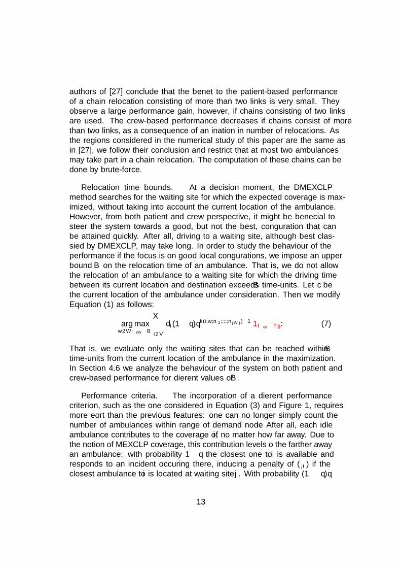
Relocation time bounds. At a decision moment, the DMEXCLPmethod searches for the waiting site for which the expected coverage is max-imized, without taking into account the current location of the ambulance.However, from both patient and crew perspective, it might be beneficial tosteer the system towards a good, but not the best, configuration that canbe attained quickly. After all, driving to a waiting site, although best clas-sified by DMEXCLP, may take long. In order to study the behaviour of theperformance if the focus is on good local configurations, we impose an upperbound B on the relocation time of an ambulance. That is, we do not allowthe relocation of an ambulance to a waiting site for which the driving timebetween its current location and destination exceeds B time-units. Let c bethe current location of the ambulance under consideration. Then we modifyEquation (1) as follows:

arg maxw∈W :τcw≤B

∑i∈V

di(1− q)qk(i,w,n1,...,n|W |)−1·1{τwi≤T}. (7)

That is, we evaluate only the waiting sites that can be reached within Btime-units from the current location of the ambulance in the maximization.In Section 4.6 we analyze the behaviour of the system on both patient andcrew-based performance for different values of B.

Performance criteria. The incorporation of a different performancecriterion, such as the one considered in Equation (3) and Figure 1, requiresmore effort than the previous features: one can no longer simply count thenumber of ambulances within range of demand node i. After all, each idleambulance contributes to the coverage of i, no matter how far away. Due tothe notion of MEXCLP coverage, this contribution levels off the farther awayan ambulance: with probability 1 − q the closest one to i is available andresponds to an incident occuring there, inducing a penalty of Φ(τji) if theclosest ambulance to i is located at waiting site j. With probability (1− q)q

13

the second closest responds, generating Φ(τj′i) penalty if this ambulance isat j′, and so on.

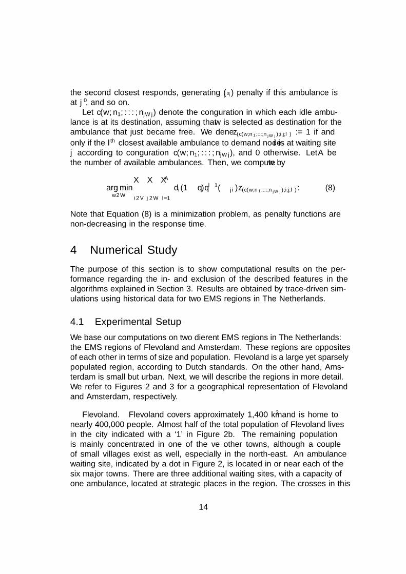
Let c(w, n1, . . . , n|W |) denote the configuration in which each idle ambu-lance is at its destination, assuming that w is selected as destination for theambulance that just became free. We define z(c(w,n1,...,n|W |),i,j,l) := 1 if and

only if the lth closest available ambulance to demand node i is at waiting sitej according to configuration c(w, n1, . . . , n|W |), and 0 otherwise. Let A bethe number of available ambulances. Then, we compute w by

arg minw∈W

∑i∈V

∑j∈W

A∑l=1

di(1− q)ql−1Φ(τji)z(c(w,n1,...,n|W |),i,j,l). (8)

Note that Equation (8) is a minimization problem, as penalty functions arenon-decreasing in the response time.

4 Numerical Study

The purpose of this section is to show computational results on the per-formance regarding the in- and exclusion of the described features in thealgorithms explained in Section 3. Results are obtained by trace-driven sim-ulations using historical data for two EMS regions in The Netherlands.

4.1 Experimental Setup

We base our computations on two different EMS regions in The Netherlands:the EMS regions of Flevoland and Amsterdam. These regions are oppositesof each other in terms of size and population. Flevoland is a large yet sparselypopulated region, according to Dutch standards. On the other hand, Ams-terdam is small but urban. Next, we will describe the regions in more detail.We refer to Figures 2 and 3 for a geographical representation of Flevolandand Amsterdam, respectively.

Flevoland. Flevoland covers approximately 1,400 km2 and is home tonearly 400,000 people. Almost half of the total population of Flevoland livesin the city indicated with a ‘1’ in Figure 2b. The remaining populationis mainly concentrated in one of the five other towns, although a coupleof small villages exist as well, especially in the north-east. An ambulancewaiting site, indicated by a dot in Figure 2, is located in or near each of thesix major towns. There are three additional waiting sites, with a capacity ofone ambulance, located at strategic places in the region. The crosses in this

14

(a) (b)

Figure 2: EMS region of Flevoland.

figure mark the two hospitals in Flevoland. We aggregate the region into93 demand nodes, based on 4-digit postal codes. Note that the postal codecorresponding to the dot indicated by a ‘2’ contains both a waiting site anda hospital.

Amsterdam. The EMS region containing the city of Amsterdam andits surroundings is approximately 630 km2. However, the population of Am-sterdam is three times larger than that of Flevoland: 1.2 million inhabitants.Approximately 68% lives in Amsterdam itself, while the northern part of theregion is less densely populated. Ambulance waiting sites and hospital arepresent at the dots and crosses in Figure 3, respectively. The numbers inbrackets denote the actual waiting site capacities. The region is aggregatedinto 162 postal codes, which serve as demand points. Moreover, both a wait-ing site and a hospital are present in the postal codes corresponding to dots2, 4, 5, and 11. Approximately 73% of the patients needs transportation toa hospital.

Historical data on emergency requests in the year 2011 was provided byGGD Flevoland and Ambulance Amsterdam, the ambulance service providersof Flevoland and Amsterdam, respectively. We built two traces based onthis data and simulate them in a discrete-event simulation. The trace isconstructed as follows. We consider all emergency requests occuring between7 AM and 6 PM, generally the busiest time of the day. In the trace, we

15

(a) (b)

Figure 3: EMS region of Amsterdam.

include the following incident related information:

• Time of occurence, i.e., the time of the emergency call;

• Location of occurence (postal code);

• Time spent on-scene by the ambulance;

• Hospital transfer time.

Emergency requests of which above data is not complete or infeasible areignored. We are interested in an algorithm that performes well for most days.Therefore, we classify the days for which the number of incidents falls outsidethe interval [µ−2σ, µ+2σ] as outliers, where µ and σ denote the mean numberof requests per day and the standard deviation, respectively. This results inan exclusion of two days for both regions. Moreover, we remove the last 12days of the year because the fleet capacity was inadequate. We connect theremaining 352 days such that 6 PM is followed directly by 7 AM the next dayto ensure that the ambulance system is in continuous operation. This avoids

16

that the system becomes empty over night, and thereby our aproach allowsus to obtain measurements that are close to ‘steady state’, which is what weare interested in. In the resulting trace 7,632 resp. 41,996 incidents occur inFlevoland and Amsterdam, respectively. This yields an hourly arrival rateof 1.97 resp. 10.84 emergency requests. Moreover, around 87% resp. 73%of the patients needs transportation to a hospital. The average busy timeof an ambulance is 0.74 resp. 0.73 hours, excluding relocation time afterthe transfer. In order to ensure an out-of-sample validation, we estimate thedemand probabilities per postal code based on the year 2010, and not 2011.

In our simulation, the closest idle ambulance always responds to the in-cident. If no ambulance is available, the call enters a queue. Once an ambu-lance becomes available from service again, it is immediately dispatched tothe longest waiting request. Moreover, if a patient needs transportation toa hospital, the closest hospital is selected. In the simulation model, we usetravel times estimated by the RIVM4, which provided us tables containingtravel times between each pair of postal codes in the regions of considera-tion. We refer to [15] for a more detailed description on the travel time modelused for the estimation of these travel times. We interpret the travel timesin these tables as the arc lengths τ (1). The travel times τ (2) are obtainedby multiplying τ (1) with a multiplication factor of 10

9. We do not simulate a

dispatch time or pre-trip delay.We test the performance of the methods considered on the following seven

statistics:

1. Percentage on time: the fraction of requests responded to within the re-sponse time threshold of 12 minutes. Actually, the statutory thresholdin The Netherlands is 15 minutes, but typically 3 minutes are reservedfor handling the phone call and the pre-trip delay. We also provideconfidence intervals.

2. Mean response time.

3. Number of relocations. This number includes the relocation of an am-bulance that just finished service as well.

4. Average relocation time. Note that this number is solely based on thetravel times τ (2) since it is not allowed to perform a relocation withoptical signals and sirens turned on.

5. Total relocation time.

4Rijksinstituut Volksgezondheid en Milieu (National Institute for Public Health andthe Environment).

17

6. Mean single coverage. Each time a relocation decision is made in thesimulation, the distribution of ambulance vehicles over waiting siteschanges. At that moment, we compute the coverage of the region asif each idle ambulance was already at its destination, based on theassumption that a demand point is covered if it is covered by at leastone ambulance (single coverage). This coverage value lasts until thetime of the next event: the arrival or completion of a call. The reportedpercentage is a time-average over the complete simulation horizon.

7. Mean MEXCLP coverage. The computation of this value is similar tothe computation of the mean single coverage, but we use the MEXCLPcoverage instead.

The number of ambulances we assume to be on duty is smaller than thenumber in reality. This is because we focus on the urgent transports, whilethe ambulance providers in practice sometimes also respond to non-urgentrequests using the same vehicles. These non-urgent requests are a taxi-liketransports of patients that are not able to travel to the hospital themselves.These requests are of a different nature, since they can usually be scheduledin advance, and therefore we do not wish to mix the two cases in our analysis.In our implementation, we choose a fleet size such that a ‘good’ policy givesa performance of a magnitude that is realistic for practical purposes: 10 resp.18 ambulances for Flevoland resp. Amsterdam. Busy fractions q = 0.1716resp. q = 0.4991 are computed by dividing the total patient-related work bythe total duty time of all ambulances.

4.2 Original DMEXCLP method

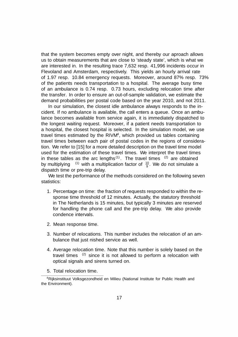
In this section, we report results for both regions of interest, Flevoland andAmsterdam, of the original DMEXCLP method, as proposed in [14]. More-over, we compare these results to the static policy according to the MEXCLPsolution: each ambulance returns to its home base station when newly idle.Results are listed in Table 1.

A large performance improvement in terms of late arrivals can be observedin Table 1 for the Amsterdam region. This quantity decreased from on av-erage 6.19% to 4.10%, a difference of 2.09 percentage point and a decreaseof 33.76%, even outperforming the performance gain reported in the originalarticle ([14], for the region of Utrecht). However, the performance gain re-garding this criterion is small for Flevoland: a difference of 0.11 percentagepoint, which is a decrease of only 2.1%. Moreover, the confidence boundsfor this region overlap almost entirely. In addition, the gaps in mean singlecoverage and mean MEXCLP coverage between the static and DMEXCLP

18

Performance Indicators Flevoland AmsterdamStatic DMEXCLP Static DMEXCLP

Percentage on time 94.86% 94.97% 93.81% 95.90%Lower Bound 95%-CI 94.28% 94.45% 93.21% 95.40%Upper Bound 95%-CI 95.45% 95.49% 94.43% 96.41%Mean response time 304 s 303 s 371 s 329 sNumber of relocations 7,632 7,632 41,311 41,391Average relocation time 437 s 814 s 384 s 585 sTotal relocation time 927 h 1,726 h 4,410 h 6,725 hMean single coverage 96.26% 96.63% 97.64% 98.81%Mean MEXCLP coverage 93.24% 93.57% 93.43% 95.78%

Table 1: Simulation results for the static and DMEXCLP policy, based on7,632 and 41,966 incidents in 2011, with 10 and 18 ambulances, respectively.

policy are much smaller for Flevoland. This was already foreseen in [14], anda possible explanation for this phenomenon is given: the DMEXCLP methodis designed for busy areas in particular. The hourly arrival rate of incidentsin Flevoland is much smaller compared to the urban Amsterdam region. Asa consequence, there are fewer relocation moments, inducing a smaller per-formance improvement. (In the next subsection, we allow additional decisionmoments.)

In contrast to Flevoland, the number of ambulance relocations in Ams-terdam does not equal the number of incidents. This is explained by the factthat in Amsterdam sometimes the situation occurs that none of the ambu-lances is available for a reported incident. As soon as an ambulance finishesservice of a patient, it is immediately dispatched to a waiting call. Thisis not recorded as a relocation and hence, the number of relocations doesnot necessarily equal the number of incidents. Based on Table 1 one cancompute that the total number of incidents for which no ambulance was im-mediately available, equals 655 and 575 for the static and DMEXCLP policy,respectively.

Note that both the mean single and MEXCLP coverage performance in-dicators serve as an estimate of the number of calls for which the responsetime treshold is achieved. As observed in Table 1, the mean single coverageis an optimistic approximation of this quantity for both policies, as expected.After all, ambulance unavailability is not taken into account in the conceptof single coverage. The relative gap between mean single coverage and per-centage on time is smaller for Flevoland, compared to Amsterdam, for bothpolicies. This is not very surprising, since in Flevoland the overlap in cover-

19

age of multiple ambulances is very small: the distances between the 6 largetowns generally exceed the time threshold. Only multiple ambulances parkedat one and the same waiting site do provide overlapping coverage. Further-more, the busy fraction in Flevoland is relatively low. Therefore, the errormade when ignoring ambulance unavailability will also be small.

Even for Flevoland, the mean MEXCLP coverage over time turns out tobe a more accurate approximation for the on time arrivals, although thereis still a small gap. Note that for Amsterdam the mean MEXCLP coverageis closer to the observed percentage on time. We conjecture that this isprobably due to the way in which the coverage is computed. As explainedearlier, we compute this based on the configuration in which each ambulanceis at its destination. For Amsterdam, the time until the desired ambulanceconfiguration is attained is much shorter as a consequence of both a smallerarea and a larger number of waiting sites, compared to Flevoland. Therefore,the mean MEXCLP coverage is a more accurate estimate on the percentageon time for Amsterdam than for Flevoland.

4.3 Decision Moments

As explained in Section 3.3, we allow the dispatcher to perform an ambulancerelocation if the number of available ambulances decreases, just after thedispatch. As a consequence the number of opportunities to steer the systemis multiplied by 2. Results are displayed in Table 2. In this table and theforthcoming ones, the default policy is the DMEXCLP policy explained inSection 3.1, without any additional features. This policy outperforms thestatic policy, commonly used as benchmark policy in ambulance literature,on the most important performance indicators, as Table 1 underlines.

For the percentage on time criterion, we observe an increase of 0.63 and0.45 percentage point for Flevoland and Amsterdam, respectively. That is,the number of late arrivals decreased with 12.53% and 10.98%. We concludethat for Flevoland, the effect of adding additional relocation moments is muchlarger than the original effect of changing from static ambulance planning tothe default move-up method (which was 2.1%). For Amsterdam, the defaultmove-up already had a large effect, hence the added benefit of additionalrelocation moments seems smaller in comparison.

Surprisingly, the results on mean response times do not concur with thoseon the late arrivals criterion: in Flevoland, a performance gain of only 1.64%is achieved. In contrast, the mean response time in Amsterdam decreaseswith 7.44%. A possible explanation for this behaviour is as follows: sinceFlevoland is a rural region, an ambulance travelling between two waitingsites provides no or very little coverage. After all, few people live in the areas

20

Performance Indicators Flevoland AmsterdamDefault5 Moments Default Moments

Percentage on time 94.97% 95.60% 95.90% 96.35%Lower Bound 95%-CI 94.45% 95.06% 95.40% 95.87%Upper Bound 95%-CI 95.49% 96.14% 96.41% 96.83%Mean response time 303 s 299 s 329 s 306 sNumber of relocations 7,632 13,308 41,391 76,161Average relocation time 814 s 1,367 s 585 s 730 sTotal relocation time 1,726 h 5,054 h 6,725 h 15,453 hMean single coverage 96.63% 97.34% 98.81% 99.10%Mean MEXCLP coverage 93.57% 94.61% 95.78% 96.76%

Table 2: Simulation results for Flevoland and Amsterdam, based on 7,632and 41,966 incidents in 2011, with 10 and 18 ambulances, respectively.

between the cities, cf. Figure 2. In contrast, a large part of the Amsterdamregion is urban, cf. Figure 3. In an urban area, an ambulance performing arelocation drives through a densely populated area, being able to respond toan incoming call in that area quickly. As the number of ambulance relocationsalmost doubles for both regions, this effect will be largest in Amsterdam,resulting in a relative large decrease in mean response time.

In the crew-related performance indicators, we observe both an increasein number of relocations and average relocation time. As a consequence, thetotal relocation time is more than doubled. A trade-off between patient- andcrew-based performance, which is the subject of [27], is clearly visible hereas well. The question arises whether this large increase outweighs the gainin patient-based performance. It is up to the ambulance service provider todecide on this, but we suspect that the answer depends on the daily workloadof the crew. As this is typically lower in rural regions, we expect those EMSproviders to be more open to additional relocation moments.

Note that for Amsterdam the mean MEXCLP coverage is now an opti-mistic estimate for the number of calls responded to within the time thresh-old, if more decision moments are allowed. We conjecture that this is due tothe ‘intended configuration’, on which the computation of the mean MEX-CLP coverage is based, changes so often that only a small fraction of theseconfigurations is actually attained. That is, the steering towards the in-tended ambulance configuration is often interrupted by a new decision mo-ment, which results in a different desired configuration.

5In this table and the forthcoming ones, the default policy is the DMEXCLP policyexplained in Section 3.1, without any additional features.

21

4.4 Hospitals

In this section, we explore the differences in performance if ambulances trans-ferring patients at hospitals are taken into account. We do this in two ways.First, we consider the data obtained via the ambulance service providers andfit a distribution on the busy times of an ambulance at a hospital. As men-tioned in Section 3.3, we plug in the expected remaining service time in theformula given the hospital time already elapsed. As an alternative approach,we simulate the system in which we have ‘perfect information’ regarding thehospital transfer time. We assume that we know this time when an am-bulance arrives at the hospital, which results in a deterministic remainingservice time. This approach clearly is a rather optimistic approach, and itcan be interpreted as a bound on the knowledge that one can have on the re-maining service time. However, this approach is more realistic than one mightexpect at first glance, as ambulance crews and dispatchers in The Nether-lands are able to estimate the hospital transfer time rather accurately6. Inparticular, hospitals in The Netherlands do not suffer from queues buildingup at an emergency department, in contrast to North America where theaverage transfer time can be very large and highly variable, cf. [7].

We estimate the service time at a hospital by a Weibull distribution, forboth regions. In our experience, this distribution provides a rather accurateapproximation. Moreover, a Weibull distribution for this quantity was alsoused in both [18] and [26]. The means of the fitted distributions are 966seconds and 1,160 seconds for Flevoland and Amsterdam, respectively. Thedifferences in mean are probably explained by the fact that the hospitals inAmsterdam are typically larger, and thus the ambulance personnel spendsmore time on the transport of the patient to the appropriate departmentwithin the hospital. Based on the Weibull distributions, we calculate the ex-pected remaining transfer time for each possible value of service time alreadyelapsed.

In Table 3, we listed simulated results on the assumption of Weibulldistributed transfer times and perfect information, and we compare those tothe default policy explained above. We observe neither an increase nor adecrease in the patient-related performance indicators in the Weibull case.A small decrease in average relocation time can be noted, which has a smalleffect on the total relocation time as well. Based on these observations,one might conclude that the inclusion of ambulances busy at a hospital inthe algorithm in the way described in Section 3.3 does not influence theperformance.

Alternatively, the Weibull distribution used for the estimation of the

6as we have learned from discussions with dispatchers and management.

22

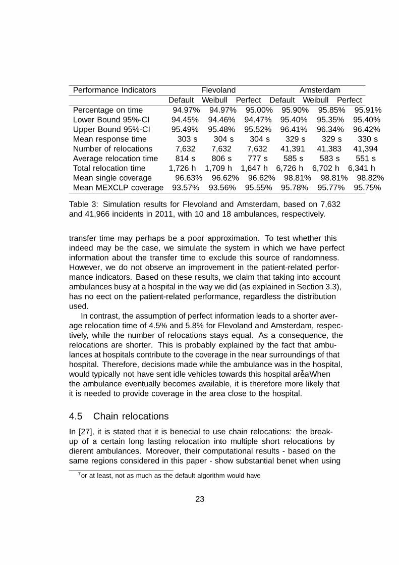
Performance Indicators Flevoland AmsterdamDefault Weibull Perfect Default Weibull Perfect

Percentage on time 94.97% 94.97% 95.00% 95.90% 95.85% 95.91%Lower Bound 95%-CI 94.45% 94.46% 94.47% 95.40% 95.35% 95.40%Upper Bound 95%-CI 95.49% 95.48% 95.52% 96.41% 96.34% 96.42%Mean response time 303 s 304 s 304 s 329 s 329 s 330 sNumber of relocations 7,632 7,632 7,632 41,391 41,383 41,394Average relocation time 814 s 806 s 777 s 585 s 583 s 551 sTotal relocation time 1,726 h 1,709 h 1,647 h 6,726 h 6,702 h 6,341 hMean single coverage 96.63% 96.62% 96.62% 98.81% 98.81% 98.82%Mean MEXCLP coverage 93.57% 93.56% 95.55% 95.78% 95.77% 95.75%


transfer time may perhaps be a poor approximation. To test whether thisindeed may be the case, we simulate the system in which we have perfectinformation about the transfer time to exclude this source of randomness.However, we do not observe an improvement in the patient-related perfor-mance indicators. Based on these results, we claim that taking into accountambulances busy at a hospital in the way we did (as explained in Section 3.3),has no effect on the patient-related performance, regardless the distributionused.

In contrast, the assumption of perfect information leads to a shorter aver-age relocation time of 4.5% and 5.8% for Flevoland and Amsterdam, respec-tively, while the number of relocations stays equal. As a consequence, therelocations are shorter. This is probably explained by the fact that ambu-lances at hospitals contribute to the coverage in the near surroundings of thathospital. Therefore, decisions made while the ambulance was in the hospital,would typically not have sent idle vehicles towards this hospital area7. Whenthe ambulance eventually becomes available, it is therefore more likely thatit is needed to provide coverage in the area close to the hospital.

4.5 Chain relocations

In [27], it is stated that it is beneficial to use chain relocations: the break-up of a certain long lasting relocation into multiple short relocations bydifferent ambulances. Moreover, their computational results - based on thesame regions considered in this paper - show substantial benefit when using

7or at least, not as much as the default algorithm would have

23

Performance Indicators Flevoland AmsterdamDefault Chains Default Chains

Percentage on time 94.97% 94.89% 95.90% 95.89%Lower Bound 95%-CI 94.45% 94.39% 95.40% 95.35%Upper Bound 95%-CI 95.49% 95.39% 96.41% 96.43%Mean response time 303 s 306 s 329 s 331 sNumber of relocations 7,632 11,619 41,391 64,998Average relocation time 814 s 563 s 585 s 415 sTotal relocation time 1,726 h 1,816 h 6,726 h 7,490 hMean single coverage 96.63% 96.57% 98.81% 98.78%Mean MEXCLP coverage 93.57% 93.51% 95.78% 95.72%


two links instead of one, but more than two links appears to be redundant.We simulate the system according to this regime: a relocation is decomposedinto a chain relocation of length two if this reduces the time until the newconfiguration is attained. Results are displayed in Table 4.

Although the time until the desired configuration is attained is decreased,we do not observe a gain on the patient-related performance criteria. Instead,even a slight deterioration can be seen in Table 4. This contradicts thefindings of [27]. This is probably due to the fact that in [27] extra decisionmoments are allowed, as considered in Sections 3.3 and 4.3. In Section 4.7,we will study the effect of the combination of extra decision moments andchain relocations.

As expected, the number of relocations increases a lot in a regime in whichchain relocations are allowed. In approximately 52% of the times an ambu-lance becomes available, an additional ambulance is relocated in Flevoland.This percentage for Amsterdam is approximately 56%. One would expectthis percentage for Amsterdam to be much higher, as more waiting sites andambulances are present in Amsterdam. Hence, there are more possibilitiesto set up a chain relocation. However, the distances between waiting sitesin this region are shorter, whereby the gain of chain relocations is probablysmaller. This is also reflected in the average relocation time. Of course, thisquantity decreases tremendeously for both regions, but the relative decreasefor Flevoland is much larger, as a consequence of the longer distances betweenwaiting sites.

24

4.6 Relocation time bounds

As explained in Section 3.3, we impose different bounds on the relocation timeof an ambulance. This bound is given by the variable B. If there is no waitingsite that can be reached within B minutes exists, the ambulance travels tothe nearest waiting site. For B = 0, the obtained policy is equivalent tothis ‘nearest base’-policy. In Figures 4 and 5 we show results on the mostimportant patient- and crew-related performance indicators: percentage ontime and total relocation time, as function of B. In Tables 5 and 6 resultson all performance indicators are displayed for B = 0, 10, 20, 30 minutes.

Figure 4: Percentage on time as function of B.

In Figure 4 we observe a large difference in the system’s behaviour. ForAmsterdam, the bound B is of little influence only: the percentage of callsreached within the time threshold is close to 95% for all levels of B. Incontrast, we see a huge improvement in performance for larger values of B inFlevoland: for B < 12 the percentage on time is below 75% and this increasesup to approximately 95%. This phenomenon has a simple explanation: it isa consequence of both the size and the number of waiting sites and hospitalsin Flevoland. The mean distances between two waiting sites are much larger,

25

Performance Indicators B = 0 min 10 min 20 min 30 minPercentage on time 74.17% 72.83% 92.28% 94.75%Lower Bound 95%-CI 73.00% 71.46% 91.49% 94.16%Upper Bound 95%-CI 75.32% 74.19% 93.08% 95.33%Mean response time 495 s 496 s 335 s 308 sNumber of relocations 7,632 7,632 7,632 7,632Average relocation time 79 s 153 s 607 s 670 sTotal relocation time 168 h 325 h 1,286 h 1,420 hMean single coverage 75.59% 74.87% 94.19% 96.42%Mean MEXCLP coverage 74.61% 73.16% 91.17% 93.33%

Table 5: Simulation results for Flevoland based on 7,632 incidents in 2011,with 10 ambulances. Results on relocation bounds 0, 10, 20, 30 minutes aredisplayed.

Performance Indicators B = 0 min 10 min 20 min 30 minPercentage on time 94.23% 96.05% 95.82% 95.90%Lower Bound 95%-CI 93.72% 95.55% 95.29% 95.40%Upper Bound 95%-CI 94.74% 96.54% 96.35% 96.40%Mean response time 323 s 322 s 330 s 329 sNumber of relocations 41,398 41,388 41,390 41,391Average relocation time 131 s 341 s 568 s 585 sTotal relocation time 1,504 h 3,919 h 6,535 h 6,726 hMean single coverage 97.69% 98.63% 98.80% 98.81%Mean MEXCLP coverage 93.60% 95.55% 95.75% 95.78%

Table 6: Simulation results for Amsterdam based on 41,966 incidents in 2011,with 18 ambulances. Results on relocation bounds 0, 10, 20, 30 minutes aredisplayed.

26

Figure 5: Total relocation time as function of B.

so for small values of B there are few possibilities for the destination of anambulance after a service completion. Moreover, since there are only twohospitals in the region and approximately 75% of the ambulances becomeavailable there, relocations to waiting sites 3, 4, 5 and 6 do not take place.

Another interesting point is the drop between B = 7 and B = 8 forFlevoland. This behaviour is due to one relocation in particular: the reloca-tion time for an ambulance between the hospital in city 1 and waiting site7 is exactly 7.5 minutes. Thus, for B = 7, an ambulance becoming free atthis hospital moves to waiting site 1, regardless of the number of ambulancesalready present there. In contrast, for B = 8, this ambulance travels towaiting site 7, if unoccupied. The benefit of covering the southeastern partis outweighed by the performance loss in city 1. This aspect can be observedin the coverages displayed in Table 5 as well.

All large jumps are easily explained as well: the jump at B = 12 is dueto the allowance of a relocation from 2 to 9; the one at B = 18 is due to therelocation from 1 to 3. If B = 20, it is now allowed to relocate an ambulancefrom 2 to both 4 and 5 as well. Finally, waiting site 6 can be reached from 2if B exceeds 23 minutes. These jumps are largely visible in Figure 5 as well.

27

Moreover, the large increase in total relocation time at B = 36 is due thefact that relocations from 1 to 4 and 6 both are acceptable now.

The pattern for Amsterdam is of different shape: the best performance isachieved for 10 ≤ B ≤ 13, although the differences are minor. Apparently,it is beneficial to the performance if one chooses a relatively close waitingsite if an ambulance is newly free. That is, a local optimum that can bereached quickly performs better than a global one for which it takes long untilthat configuration is attained. A possible explanation for this phenomenonis the large number of events and thus decision moments in Amsterdam.This behaviour is also reflected in Table 6: the coverage levels belongingto B = 30 are higher than for B = 10, although B = 10 yields a largerpercentage on time. Note that there is also a reduction in mean responsetime of approximately 2.1% for B = 10 compared to B = 30.

4.7 Combinations

In this section, we will combine different highly promising features and testthe method for both regions. Moreover, we compare the performance withtwo other policies: the penalty heuristic of [27] summarized in Section 3.2and a compliance table policy. A compliance table indicates the desired con-figuration for each number of available ambulances. We test the followingcombinations and methods:

1. DMEXCLP with extra decision moments, with chain relocations, with-out taking into account ambulances busy at hospitals.

2. DMEXCLP with extra decision moments, with chain relocations; busytime at the hospital follows the Weibull distribution considered in Sec-tion 4.4.

3. Similar to 2, but now we have perfect information about the transfertimes.

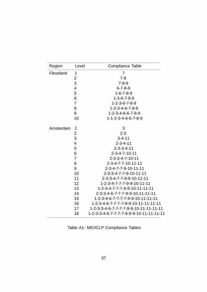
4. Compliance table: to obtain the desired configurations per numberof available ambulances, we solve multiple MEXCLP problems. Thecomputed compliance tables are displayed in Table A1. We do notallow chain relocations.

5. The same compliance table is used, but we allow chain relocations now.

6. Penalty heuristic, (see Section 3.2).

28

Performance Indicators FlevolandCombination: 1 2 3 4 5 6Percentage on time 96.24% 96.24% 96.27% 95.15% 95.41% 94.22%Lower Bound 95%-CI 95.79% 95.77% 95.82% 94.55% 94.82% 93.64%Upper Bound 95%-CI 96.69% 96.71% 96.71% 95.76% 96.01% 94.80%Mean response time 292 s 292 s 292 s 305 s 307 s 288 sNumber of relocations 24,747 24,408 23,481 29,518 49,466 22,047Average relocation time 774 s 766 s 766 s 991 s 688 s 599 sTotal relocation time 5,318 h 5,196 h 4,997 h 8,126 h 9,447 h 3,671 hMean single coverage 97.34% 97.34% 97.34% 97.24% 97.18% 97.43%Mean MEXCLP coverage 94.61% 94.60% 94.58% 94.33% 94.27% 93.24%

Table 7: Simulation results for different combinations for Flevoland, basedon 7,632 in 2011, with 10 ambulances.

Performance Indicators AmsterdamCombination: 1 2 3 4 5 6Percentage on time 97.23% 97.21% 97.26% 95.60% 95.36% 97.10%Lower Bound 95%-CI 96.82% 96.77% 96.84% 95.11% 94.82% 96.68%Upper Bound 95%-CI 97.64% 97.66% 97.67% 96.09% 95.90% 97.51%Mean response time 303 s 302 s 302 s 322 s 325 s 283 sNumber of relocations 132,918 132,530 127,467 315,629 414,782 129,988Average relocation time 440 s 439 s 424 s 456 s 372 s 457 sTotal relocation time 16,258 h 16,172 h 15,026 h 40,009 h 43,169 h 16,486 hMean single coverage 99.12% 99.11% 99.13% 99.10% 99.00% 99.34%Mean MEXCLP coverage 96.79% 96.78% 96.75% 96.60% 96.60% 95.62%

Table 8: Simulation results for different combinations for Amsterdam, basedon 41,966 in 2011, with 18 ambulances.

29

Results are displayed in Tables 7 and 8. Although allowing chain reloca-tions initially did not result in better performance regarding the percentageon time criterion, as observed in Table 4, it is a valuable addition if it is com-bined with the allowance of extra decision moments, for both regions. If wecompare Table 2, which shows the best performance concerning this criterionup to now, with the first columns in Tables 7 and 8, we see that performanceimprovements of 0.64 resp. 0.88 percentage points are achieved for Flevolandand Amsterdam, respectively. That is, the number of late arrivals decreasedwith 14.55% and 24.11%. This behaviour is probably explained by the fol-lowing reason: it is more likely that a poor ambulance configuration arisesjust after the dispatch than when an ambulance becomes available. There-fore, at that decision moment, it is more important to attain the desiredconfiguration quickly. This is achieved by using chain relocations, explainingthe difference in performance.

If we compare columns 1, 2 and 3 in Tables 7 and 8, we barely see anydifferences in patient-based performance. This underlines the observations inSection 4.4. Results on crew-based performance are similar to those obtainedin Section 4.4 as well.

Note that the DMEXCLP method in which extra decision moments andchain relocations are allowed (columns 1, 2 and 3 in Tables 7 and 8) per-forms significantly better than the MEXCLP compliance table policy on thepercentage on time criterion. Moreover, it also outperforms the compliancetable on the crew-related performance indicators. We conclude that althoughallowing for chain relocations in the compliance table policy (column 5) re-duces the average relocation time, this effect is outweighed by the dramaticincrease in number of relocations.

Both the DMEXCLP method with its features and the MEXCLP com-pliance table policies are quite consistent in their behaviour for both regions,although the regions of consideration differ heavily. The penalty heuristic,however, shows different performance: it performs comparably to the DMEX-CLP method for Amsterdam, while for Flevoland it is outperformed even bythe compliance table policy. A simple explanation for this phenomenon hasits roots in the concept of single coverage: the method tries to maximize thedemand covered at least once. This results in the relocation of ambulancesto each outskirt of the region in Flevoland. As a consequence, it ‘misses’ asecond call occuring shortly after a first one in one of the two large cities,in which approximately 75% of the incidents occur: ambulances located inthe towns 3, 4, 5, and 6 are not able to arrive in cities 1 and 2 within thetime threshold, resulting in a worse performance. In contrast, the distancesfrom waiting sites to postal codes are much shorter in Amsterdam, and asa side effect, a postal code is typically automatically multiple covered, even

30

the algorithm focuses on maximizing single coverage.Note that the penalty heuristic does not focus on coverage solely, but

it uses the penalty function of Equation (3). One can observe in Tables 7and 8 that minimizing the average response time is included in this penaltyfunction as well, as this method yields the shortest mean response time forboth regions. In addition, the single coverage concept is used in the penaltyheuristic. As a consequence, the mean single coverage levels are highest forthe penalty heuristic, at the expense of a lower mean MEXCLP coverage.

If we modify the DMEXCLP method of [14] in such a way that extra deci-sion moments and chain relocations are allowed, we observe an improvementover other policies on most performance indicators if the coverage penaltyfunction is used. In the next section, we consider different penalty functionsand explore the performance of the DMEXCLP method with additional fea-tures.

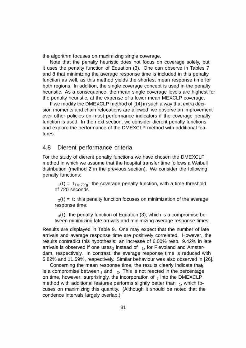
4.8 Different performance criteria

For the study of different penalty functions we have chosen the DMEXCLPmethod in which we assume that the hospital transfer time follows a Weibulldistribution (method 2 in the previous section). We consider the followingpenalty functions:

• Φ1(t) = 1{t>720}: the coverage penalty function, with a time thresholdof 720 seconds.

• Φ2(t) = t: this penalty function focuses on minimization of the averageresponse time.

• Φ3(t): the penalty function of Equation (3), which is a compromise be-tween minimizing late arrivals and minimizing average response times.

Results are displayed in Table 9. One may expect that the number of latearrivals and average response time are positively correlated. However, theresults contradict this hypothesis: an increase of 6.00% resp. 9.42% in latearrivals is observed if one uses Φ2 instead of Φ1, for Flevoland and Amster-dam, respectively. In contrast, the average response time is reduced with5.82% and 11.59%, respectively. Similar behaviour was also observed in [26].

Concerning the mean response time, the results clearly indicate that Φ3

is a compromise between Φ1 and Φ2. This is not reflected in the percentageon time, however: surprisingly, the incorporation of Φ3 into the DMEXCLPmethod with additional features performs slightly better than Φ1, which fo-cuses on maximizing this quantity. (Although it should be noted that theconfidence intervals largely overlap.)

31

Performance Indicators Flevoland AmsterdamΦ1(t) Φ2(t) Φ3(t) Φ1(t) Φ2(t) Φ3(t)

Percentage on time 96.24% 95.96% 96.31% 97.21% 96.92% 97.32%Lower Bound 95%-CI 95.77% 95.48% 95.84% 96.77% 96.53% 96.95%Upper Bound 95%-CI 96.71% 96.45% 96.77% 97.66% 97.32% 97.70%Mean response time 292 s 275 s 285 s 302 s 267 s 282 sNumber of relocations 24,408 24,287 26,122 132,530 134,113 134,162Average relocation time 766 s 727 s 744 s 439 s 418 s 424 sTotal relocation time 5,197 h 4,907 h 5,401 h 16,173 h 15,580 h 15,813 hMean single coverage 97.34% 97.31% 97.35% 99.11% 98.99% 99.15%Mean MEXCLP coverage 94.60% 94.09% 94.59% 96.78% 96.24% 96.80%


5 Conclusion

In this paper, we studied the implementation of several aspects and featurespresent in [27] in the dynamic relocation method proposed in [14]. Next, Wedraw conclusions and make recommendations.

Based on the results in Table 9, we would suggest to use Φ3(t) in aDMEXCLP environment. However, we want to note that Φ1(t) makes fora fine alternative, as the results only differ slightly (7 to 20 seconds for theaverage response time). A reason to choose Φ1(t) could be to make it easierto explain the behaviour of the system to EMS management and/or crew.

Adding extra decision moments (i.e., also relocating when a vehicle isdispatched to an incoming incident) is something we highly recommend inrural regions. We draw this conclusion based on the results in Table 2. Forurban regions, we consider this an optional extra, that may be implementedif the region is willing to increase the crew’s workload. Moreover, we recom-mend the use of chain relocations only if these extra decision moments areadded. After all, Table 4 shows that no performance gain is achieved, whilethe workload on the crew is much higher. In contrast, if extra decision mo-ments are added, the effect of chain relocations on the performance is muchlarger, cf., Tables 7 and 8.

When it comes to ambulances involved in a drop-off at a hospital, ourinitial recommendation is to ignore them (in terms of coverage provided).The reason for this, is that including them makes the move-up somewhatharder to implement (and explain), while it does not benefit the patients.An exception to this rule could be, when an EMS crew struggles with theirworkload: in that case, including the ambulances at hospital could be worth-

32

while, because it slightly reduces the relocation times (as seen in Table 3).Before implementing any ambulance move-up policy, we have one final

– and very important – recommendation. Perform simulation experimentsin order to get a realistic idea of what effect the move-up policy has onresponse times. Keep in mind that every region is different, and that it is veryhard to predict effects in a system as complex and stochastic as ambulanceservices. Mathematical models should be used with care in complex systemsin practice: in our opinion simulation is an important tool that can trulycapture the behaviour of the system.

Acknowledgements

We would like to thank the ambulance service providers of the EMS regionsof Flevoland, GGD Flevoland, and Amsterdam, Ambulance Amsterdam, forproviding data. In addition, we are grateful to the RIVM for providing thetravel times for ambulances in the EMS regions considered in the numericalstudy. This research was financed in part by Technology Foundation STWunder contract 11986, which we gratefully acknowledge.

References

[1] R. Alanis, A. Ingolfsson, and B. Kolfal. A Markov chain model for anEMS system with repositioning. Production and Operations Manage-ment, 22(1):216–231, 2013.

[2] T. Andersson and P. Varbrand. Decision support tools for ambulancedispatch and relocation. The Journal of the Operational Research Soci-ety, 58(2):195–201, 2007.

[3] R. Batta, J. Dolan, and N. Krishnamurthy. The maximal expected cover-ing location problem: Revisited. Transportation Science, 23(4):277–287,1989.

[4] V. Belanger, A. Ruiz, and P. Soriano. Recent advances in emergencymedical services management. 2015.

[5] L. Brotcorne, G. Laporte, and F. Semet. Ambulance location and relo-cation models. European Journal of Operational Research, 147:451–463,2003.

[6] R.E. Burkhard, M. Dell’Amico, and S. Martello. Assignment Problems,chapter 6. SIAM, Philadelphia, 2009.

33

[7] A. Carter, J. Gould, P. Vanberkel, J. Jensen, J. Cook, S. Carrigan,M. Wheatley, and A. Travers. Offload zones to mitigate emergency med-ical services EMS offload delay in the emergency department: a processmap and hazard analysis. Canadian Journal of Emergency Medicine,pages 1–9, 2015.

[8] M. Daskin. The maximal expected covering location model: Formula-tion, properties, and heuristic solution. Transportation Science, 17:48–70, 1983.

[9] D. Degel, L. Wiesche, S. Rachuba, and B. Werners. Time-dependentambulance allocation considering data-driven empirically required cov-erage. Health Care Management Science, 18(4):444–458, 2015.

[10] E. Erkut, A. Ingolfsson, and G. Erdogan. Ambulance location for max-imum survival. Naval Research Logistics, 55(1):42–58, 2008.

[11] M. Gendreau, G. Laporte, and F. Semet. Solving an ambulance locationmodel by tabu search. Location Science, 5(2):75–88, 1997.

[12] M. Gendreau, G. Laporte, and F. Semet. A dynamic model and par-allel tabu search heuristic for real-time ambulance relocation. Parallelcomputing, 27(12):1641–1653, 2001.

[13] M. Gendreau, G. Laporte, and F. Semet. The maximal expected cover-age relocation problem for emergency vehicles. Journal of the OperationsResearch Society, 57:22–28, 2006.

[14] C.J. Jagtenberg, S. Bhulai, and R.D. van der Mei. An efficient heuristicfor real-time ambulance redeployment. Operations Research for HealthCare, 4:27 – 35, 2015.

[15] G. Kommer and S. Zwakhals. Referentiekader spreiding en beschik-baarheid ambulancezorg 2008, 2008.

[16] X. Li, Z. Zhao, X. Zhu, and T. Wyatt. Covering models and optimiza-tion techniques for emergency response facility location and planning:a review. Mathematical Methods of Operations Research, (74):281–310,2011.

[17] M. Maleki, N. Majlesinasab, and M. Mehdi Sepehri. Two new modelsfor redeployment of ambulances. Computers & Industrial Engineering,78:271–284, 2014.

34

[18] M. Maxwell, M. Restrepo, S. Henderson, and H. Topaloglu. Approxi-mate dynamic programming for ambulance redeployment. INFORMSJournal on Computing, 22(2):266–281, 2010.

[19] J. Naoum-Sawaya and S. Elhedhli. A stochastic optimization model forreal-time ambulance redeployment. Computers & Operations Research,40:1972–1978, 2013.

[20] H. Rajagopalan, C. Saydam, and J. Xiao. A multiperiod set coveringlocation model for dynamic redeployment of ambulances. Computers &Operations Research, 35(3):814 – 826, 2008.

[21] J.F. Repede and J.J. Bernardo. Developing and validating a decisionsupport system for location emergency medical vehicles in Louisville,Kentucky. European Journal of Operational Research, 75(3):567–581,1994.

[22] V. Schmid. Solving the dynamic ambulance relocation and dispatchingproblem using approximate dynamic programming. European Journalof Operational Research, 219:611–621, 2012.

[23] V. Schmid and K. Doerner. Ambulance location and relocation prob-lems with time-dependent travel times. European Journal of OperationalResearch, 207(3):1293–1303, 2010.

[24] K. Sudtachat, M.E. Mayorga, and L.A Mclay. A nested-compliance tablepolicy for emergency medical service systems under relocation. Omega,58:154–168, 2016.

[25] T.C. van Barneveld. The minimum expected penalty relocation prob-lem for the computation of compliance tables for ambulance vehicles.INFORMS Journal on Computing. To appear.

[26] T.C. van Barneveld, S. Bhulai, and R.D. van der Mei. A dynamic am-bulance management model for rural areas. Health Care ManagementScience, 2015. doi 10.1007/s10729-015-9341-3.

[27] T.C. van Barneveld, S. Bhulai, and R.D. van der Mei. The ef-fect of ambulance relocations on the performance of ambulance ser-vice providers. European Journal of Operational Research, 2016. doi10.1016/j.ejor.2015.12.022.

[28] P.L. van den Berg and K. Aardal. Time-dependent MEXCLP withstart-up and relocation cost. European Journal of Operational Research,242(2):383–389, 2015.

35

[29] L. Zhang. Simulation Optimisation and Markov Models for DynamicAmbulance Redeployment. PhD thesis, The University of Auckland,2012.

Appendix A MEXCLP Compliance Tables

36

Region Level Compliance Table

Flevoland 1 72 7-83 7-8-94 6-7-8-95 1-6-7-8-96 1-3-6-7-8-97 1-2-3-6-7-8-98 1-2-3-4-6-7-8-99 1-2-3-4-6-6-7-8-910 1-1-2-3-4-6-6-7-8-9

Amsterdam 1 32 2-33 3-4-114 2-3-4-115 2-3-3-4-116 2-3-4-7-10-117 2-3-3-4-7-10-118 2-3-4-7-7-10-11-119 2-3-4-7-7-9-10-11-1110 2-3-3-4-7-7-9-10-11-1111 2-3-3-4-7-7-9-9-10-11-1112 1-2-3-4-7-7-7-9-9-10-11-1113 1-2-3-4-7-7-7-9-9-10-11-11-1114 2-3-3-4-6-7-7-7-9-9-10-11-11-1115 1-2-3-4-6-7-7-7-7-9-9-10-11-11-1116 1-2-3-4-6-7-7-7-7-9-9-10-11-11-11-1117 1-2-3-3-4-6-7-7-7-7-9-9-10-11-11-11-1118 1-2-3-3-4-6-7-7-7-7-9-9-9-10-11-11-11-11

Table A1: MEXCLP Compliance Tables

37

real-time ambulance relocation

Documents