Real-Time 3D Model Tracking in Color and Depth on a Single CPU Core

Wadim Kehl 1,2 Federico Tombari 2 Slobodan Ilic 2,3 Nassir Navab 2

1 Toyota Research Institute, Los Altos 2 TUM, Munich 3 Siemens R&D, Munich

wadim.kehl@tri.global

Abstract

We present a novel method to track 3D models in color

and depth data. To this end, we introduce approximations

that accelerate the state-of-the-art in region-based tracking

by an order of magnitude while retaining similar accuracy.

Furthermore, we show how the method can be made more

robust in the presence of depth data and consequently for-

mulate a new joint contour and ICP tracking energy. We

present better results than the state-of-the-art while being

much faster then most other methods and achieving all of

the above on a single CPU core.

1. Introduction

Tracking objects in image sequences is a relevant prob-

lem in computer vision with significant applications in sev-

eral fields, such as robotics, augmented reality, medical nav-

igation and surveillance. For most of these applications,

object tracking has to be carried out in 3D, i.e. an algo-

rithm has to retrieve the full 6D pose of each model in ev-

ery frame. This is quite challenging since objects can be

ambiguous in their pose and can undergo occlusions as well

as appearance changes. Furthermore, trackers must also be

fast enough in order to cover larger inter-frame motions.

In the case of 3D object tracking from color images,

the related work can be roughly divided into sparse meth-

ods that try to establish and track local correspondences

between frames [30, 15], and region-based methods that

exploit more holistic information about the object such as

shape, contour or color [18, 5], although mixtures of both

do exist [22, 2, 23]. While both directions have their re-

spective advantages and disadvantages, the latter performs

better for texture-less objects, which is our focus here. One

popular methodology for texture-less object tracking relies

on the idea of aligning the projected object contours to a

segmentation in each frame. While initially shown for ar-

bitrary shapes [4, 1], more recent works put emphasis on

tracking 3D colored models [5, 18, 31, 29].

With the advent of commodity RGB-D sensors, these

methods have then been further extended to depth images

Figure 1. We can perform reliable tracking for multiple objects

while being robust towards partial occlusions as well drastic

changes in scale. To this end, we employ contour cues and in-

terior object information to drive the 6D pose alignment jointly.

All of the above is achieved on a single CPU core in real-time.

for simultaneous tracking and reconstruction [20, 19]. In-

deed, exploiting RGB-D is beneficial since image-based

contour information and depth maps are complimentary

cues, one being focused on object borders, the other on

object-internal regions. This has been exploited for 3D ob-

ject detection and tracking [16, 9, 13, 12], as well as to im-

prove camera tracking in planar indoor environments [32].From a computational perspective, several state-of-the-

art trackers leverage the GPU for real-time performance

[20, 19, 29]. Nevertheless, there is a strong interest towards

decreasing the computational burden and generally avoid-

ing GPU usage, motivated by the fact that many relevant

applications require trackers to be light-weight [11, 17].Taking this all into consideration, we propose a frame-

work that allows accurate tracking of multiple 3D mod-

els in color and depth. Unlike related works [18, 29] our

method is lightweight, both in computation (requiring only

one CPU core) and in memory footprint. To achieve this,

we propose to pre-render a given target 3D model from var-

ious viewpoints and extract occluding contour and interior

information in an offline step. This avoids time consuming

745

online renderings and consequently results in a fast tracking

approach. Furthermore, we do not compute the terms of our

objective function densely but introduce sparse approxima-

tions which gives a tremendous performance boost, allow-

ing real-time tracking of multiple instances. While the pro-

posed contour-based tracking works well in RGB images, in

the case of available depth information, we propose two ad-

ditions: firstly, we make the color-based segmentation more

robust by incorporating cloud information and secondly, we

define a new tracking framework where a novel plane-to-

point error on cloud data and a contour error are simultane-

ously steering the pose alignment.

• As a foundation of our work, we propose to pre-render

the model view space and extract contour and interior

information in an offline step to avoid online rendering,

making our method a pure CPU-based approach.

• We evaluate all terms sparsely instead of densely

which gives a tremendous performance boost.

• Given RGB-D data, we show how to improve contour-

based tracking by incorporating cloud information into

the color contour estimation. Additionally, we present

a new joint tracking that incorporates a novel plane-

to-point error and a contour error, i.e. color and depth

points are simultaneously steering the pose alignment.

Therefore, our method can deal with challenges typi-

cally encountered in tracking as depicted in the Figure 1.

In the results section, we evaluate our approach both quan-

titatively and qualitatively and compare it to the related ap-

proaches reporting better accuracy at higher speeds.

2. Related work

We confine ourselves to the field of 3D model tracking

in color and depth. Earlier works in this field employ either

2D-3D correspondences [21, 22] or 3D edges [6, 28, 24]

and fit the model in an ICP fashion, i.e. without explicitly

computing a contour. While successive methods along this

direction managed to obtain improved performance [2, 23],

another set of works solely focused on tracking densely the

contour by evolving a level-set function [1, 5]. In particular,

Bibby et al. [1] aligned the current evolving 2D contour to a

color segmentation, and demonstrated improved robustness

when computing a posterior distribution in color space.Based on this work, the first real-time contour tracker for

3D models was presented by Prisacariu et al. [18], where

the contour is determined by projecting the 3D model with

its associated 6D pose onto the frame. Then, the align-

ment error between segmentation and projection drives the

update of the pose parameters via gradient descent. In a

follow-up work [17], the authors extend their method to si-

multaneously track and reconstruct a 3D object on a mobile

phone in real-time. They circumvent GPU rendering by

hierarchically ray-casting a volumetric representation and

speed up pose optimization by exploiting the phone’s in-

ertial sensor data. Tjaden et al. [29] build on the original

framework and extend it with a new optimization scheme

that employs Gauss-Newton together with a twist repre-

sentation. Additionally, they handle occlusions in a multi-

object tracking scenario, making the whole approach more

robust in practice. The typical problem of these methods is

their fragile segmentation based on color histograms, which

can fail easily without using an adaptive appearance model,

or when tracking in scenes where the background colors

match the objects’ colors. Based on this, [31] explores

a boundary term to strengthen contours, whereas [8] im-

proves the segmentation with local appearance models.When it comes to temporal tracking from depth data,

there are mostly only works based on energy minimization

of sparse and dense data [16, 3, 20, 19, 32, 25], or based

on learning, such as the work from Tan et al. [26, 27] and

Krull et al. [14]. Among these, the closest to us are the

works from Ren et al. [20, 19], which track and simultane-

ously reconstruct a 3D level-set embedding from depth data,

following a color-based segmentation, and Park et al. [16]

who formulate a similar joint color/depth energy to track

and reconstruct a template-based model representation.

3. Methodology

We will first introduce the notion of contour tracking in

RGB-D images. There we formalize a novel foreground

posterior probability composed of both color and cloud

data. This is followed by the complete energy formulation

over joint contour and cloud alignment. Finally, we then

explain our further contributions to boost runtime perfor-

mance via our proposed approximation schemes.

3.1. Tracking via implicit contour embeddings

In the spirit of [18, 29], we want to track a (meshed)

3D model in camera space such that its projected silhouette

aligns perfectly with a 2D segmentation in the image I :Ω → R

3 with Ω ⊂ R2 being the image domain. Given a

silhouette (i.e. foreground mask) Ωf ⊆ Ω, we can infer a

contour C to compute a signed distance field (SDF) φ s.t.

φ(x) :=

d(x,C), x ∈ Ωb

−d(x,C), x ∈ Ωf

, d(x,C) := miny∈C

||x− y||

where a pixel tells the signed distance to the closest contour

point and Ωb := Ω \ Ωf is the set of background pixels.We follow the PWP3D tracker energy formulation [18]

in which the pixel-wise (posterior) probability of a contour,

embedded as φ, given color image I , is defined as

P (φ|I) :=∏

x∈Ω

(

Hφ(x)Pf (I(x))+(1−Hφ(x)Pb(I(x)))

)

.

(1)

746

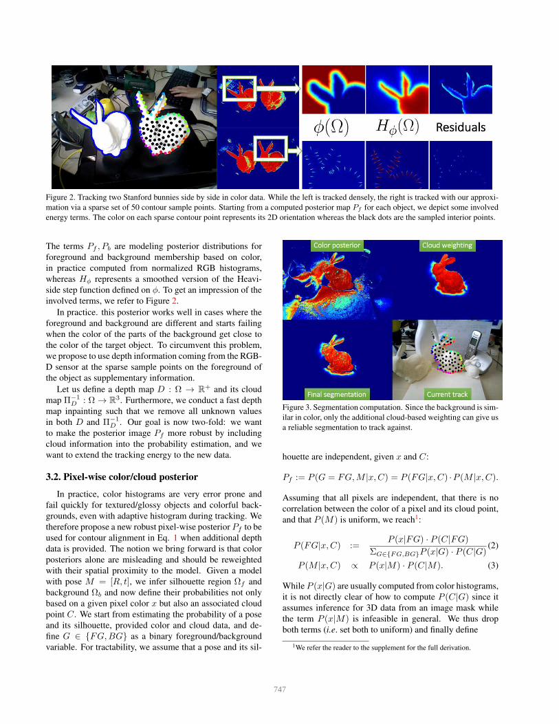
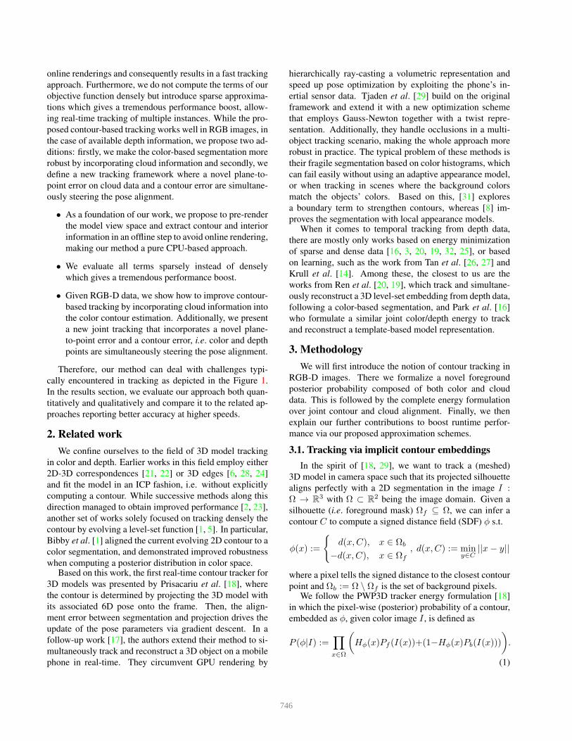
Figure 2. Tracking two Stanford bunnies side by side in color data. While the left is tracked densely, the right is tracked with our approxi-

mation via a sparse set of 50 contour sample points. Starting from a computed posterior map Pf for each object, we depict some involved

energy terms. The color on each sparse contour point represents its 2D orientation whereas the black dots are the sampled interior points.

The terms Pf , Pb are modeling posterior distributions for

foreground and background membership based on color,

in practice computed from normalized RGB histograms,

whereas Hφ represents a smoothed version of the Heavi-

side step function defined on φ. To get an impression of the

involved terms, we refer to Figure 2.

In practice. this posterior works well in cases where the

foreground and background are different and starts failing

when the color of the parts of the background get close to

the color of the target object. To circumvent this problem,

we propose to use depth information coming from the RGB-

D sensor at the sparse sample points on the foreground of

the object as supplementary information.

Let us define a depth map D : Ω → R+ and its cloud

map Π−1D : Ω → R

3. Furthermore, we conduct a fast depth

map inpainting such that we remove all unknown values

in both D and Π−1D . Our goal is now two-fold: we want

to make the posterior image Pf more robust by including

cloud information into the probability estimation, and we

want to extend the tracking energy to the new data.

3.2. Pixel­wise color/cloud posterior

In practice, color histograms are very error prone and

fail quickly for textured/glossy objects and colorful back-

grounds, even with adaptive histogram during tracking. We

therefore propose a new robust pixel-wise posterior Pf to be

used for contour alignment in Eq. 1 when additional depth

data is provided. The notion we bring forward is that color

posteriors alone are misleading and should be reweighted

with their spatial proximity to the model. Given a model

with pose M = [R, t], we infer silhouette region Ωf and

background Ωb and now define their probabilities not only

based on a given pixel color x but also an associated cloud

point C. We start from estimating the probability of a pose

and its silhouette, provided color and cloud data, and de-

fine G ∈ FG,BG as a binary foreground/background

variable. For tractability, we assume that a pose and its sil-

Figure 3. Segmentation computation. Since the background is sim-

ilar in color, only the additional cloud-based weighting can give us

a reliable segmentation to track against.

houette are independent, given x and C:

Pf := P (G = FG,M |x,C) = P (FG|x,C) ·P (M |x,C).

Assuming that all pixels are independent, that there is no

correlation between the color of a pixel and its cloud point,

and that P (M) is uniform, we reach1:

P (FG|x,C) :=P (x|FG) · P (C|FG)

ΣG∈FG,BGP (x|G) · P (C|G)(2)

P (M |x,C) ∝ P (x|M) · P (C|M). (3)

While P (x|G) are usually computed from color histograms,

it is not directly clear of how to compute P (C|G) since it

assumes inference for 3D data from an image mask while

the term P (x|M) is infeasible in general. We thus drop

both terms (i.e. set both to uniform) and finally define

1We refer the reader to the supplement for the full derivation.

747

Pf := P (C|M) · P (x|FG)

ΣG∈FG,BGP (x|G). (4)

The weighting term P (C|M), which gives the likelihood

of a cloud point to be on the model, can be computed in

multiple ways. Instead of simply taking the distance to

the model centroid, we want a more precise measure that

gives back the distance to the closest model point. Since

even logarithmic nearest-neighbor lookups would be costly

here, we use an idea first presented in [7]. One can pre-

compute a distance transform in a volume around the model

to facilitate a constant nearest-neighbor lookup function,

N(C) := argminX∈Model ||X − C||, and we exploit this

approach by bringing each scene cloud point C into the

local object frame and efficiently calculate a pixel-wise

weighting on the image plane with a Gaussian kernel:

P (c|M) := exp(−||C −N(C)||σ2

), C := R⊺ · C −R⊺t.

(5)

Here, σ = 2.5cm steers how much deviation we allow a

point to have from a perfect alignment since we want to

deal with pose inaccuracies as well as depth noise.We can see the color posterior at work plus combination

of the cloud-based weighting term in Figure 3. While the

former gives a segmentation based on appearance alone, the

latter takes complementary spatial distances into account,

rendering contour-based tracking more robust.

3.3. Joint contour and cloud tracking

We introduce the notion of a combined tracking ap-

proach where 2D contour points and 3D cloud points are

jointly driving the pose update. In essence, similar to [16],

we seek a weighted energy of the form

EJoint = EC + λEICP . (6)

where λ is balances both partial energies since they can de-

viate in the number of samples as well as numerical scale.

3.3.1 Contour energy

Assuming pixel-wise independence and taking the negative

logarithm of Eq. 1, we get a contour energy functional

EC := −∑

x∈Ω

log

(

Hφ(x)Pf (I(x))+(1−Hφ(x)Pb(I(x)))

)

.

(7)

In order to optimize the energy in respect to a change in

model pose, we employ a Gauss-Newton scheme over twist

coordinates, similarly to Tjaden et al. [29]. We define a

twist vector ξ = [tx, ty, tz, ωx, ωy, ωz]⊺ ∈ R

6 that provides

a minimal representation for our sought transformation and

its Lie algebra twist ξ ∈ se(3) as well as its exponential

mapping to the Lie group Ξ ∈ SE(3):

ξ :=

0 −ωz ωy txωz 0 −ωx ty−ωy ωx 0 tz0 0 0 0

,Ξ := exp(ξ) =

(

R t0 1

)

.

We abuse notation s.t. Ξ(X) expresses the transformation

of Ξ ∈ R4×4 applied to a 3D point X . Assuming only in-

finitesimal change in transformation we derive the energy2

in respect to a point X undergoing a screw motion ξ as

∂EC

∂ξ=

(Pf − Pb)

Hφ(Pf − Pb) + Pb

∂Hφ

∂φ

∂φ

∂x

∂π(X)

∂X

∂Ξ(X)

∂ξ.

(8)

A visualization of some terms can be seen in Figure 2.

While∂Ξ(X)

∂ξ∈ R

3×6 and∂π(X)∂X

∈ R2×3 can be written

in analytical form,∂Hφ

∂φresolves essentially to a smoothed

Dirac delta whereas ∂φ∂x

∈ R1×2 can be implemented via

simple central differences. In total, we obtain one Jacobian

Jx ∈ R1×6 per pixel and solve a least-squares problem

∇ξ = (∑

x

J⊺

xJx)−1

∑

x

Jx (9)

via Cholesky decomposition. Given the model pose M t ∈R

4×4 at time t, we update via the exponential mapping

M t+1 = exp(∇ξ) ·M t. (10)

3.3.2 ICP Energy

In terms of ICP, a point-to-plane error has been shown to

provide better and faster convergence then a point-to-point

metric. It assumes alignment of source points si (here from

a model view) to points di and normals ni at the destina-

tion (here the scene). Normals in camera space can be ap-

proximated from depth images [9] but are usually noisy and

require time. We thus propose a novel plane-to-point error

where the normals are coming from the source point set and

have been computed beforehand for each viewpoint. This

ensures a fast runtime and perfect data alignment since tan-

gent planes coincide at the optimum.Given the current pose [R, t] and closest viewpoint with

local interior points si, we transform to si = R · si + tand project each to get the corresponding scene point di :=Π−1

D (π(si)). Since we also have a local ni that we bring

into the scene, ni = R·ni, we want to retrieve Ξ minimizing

EICP := argminΞ

∑

i

(

(Ξ(si)− di) · ΞSO(ni)

)2

. (11)

2For brevity, we moved the full derivation into the supplement.

748

The difference to the established point-to-plane error is

solving for an additional rotation of the source normal ni.

Note that only the rotational part of Ξ acts on ni and we thus

omit the translational generators of the Lie algebra. Deriv-

ing in respect to ξ3, we get a Jacobian Ji ∈ R1×6 and a

residual ri for each correspondence

Ji := −[

n⊺

i

(

(si × ni) + ni × (si − di)

)⊺]

, (12)

ri := (si − di) · ni (13)

and construct a normal system to get a twist of the form

∇ξ =

(

∑

i

J⊺

i Ji

)−1∑

i

Ji · ri (14)

Altogether, we can now plug together Eqs. 7 and 11 to for-

mulate the desired energy from Eq. 6 as a joint contour and

plane-to-point alignment. Following up, we build a normal

system that contains both the ray-wise contour Jacobians

Jx from 2D image data and correspondence-wise ICP Jaco-

bians Ji from 3D cloud data:

∇ξ =

(

∑

x

J⊺

xJx+∑

i

λJ⊺

i Ji

)−1(∑

x

Jx+∑

i

√λJi·ri

)

.

(15)

Solving the above system yields a twist with which the cur-

rent pose is updated. The advantage of such a formula-

tion is that we employ entities from different optimization

problems into a common framework: while the color pix-

els minimize a projective error, the cloud points do so with

a geometrical error. These complimentary cues can there-

fore compensate for each other if a segmentation is partially

wrong or if some depth values are noisy.

3.4. Approximating for real­time tracking

Computing the SDF from Eq. 3.1 has already three

costly steps. We need a silhouette rendering Ωf of the cur-

rent model pose, an extraction of the contour C and lastly,

a subsequent distance transform embedding φ. While [29]

perform GPU rendering and couple computation of the SDF

and its gradient in the same pass to be faster, [17] perform

hierarchical ray-tracing on the CPU and extract the contour

via Scharr operators. We make two key observations:

1. Only the actual contour points are required

2. Neighboring points provide superfluous information

because of similar curvature

We thus propose a cheap yet very effective approximation

of the model render space that avoids both online rendering

and contour extraction. In an offline stage, we equidistantly

3The derivation can be found in the supplementary material.

Figure 4. Object-local 3D contour points visualized for three view-

points on the unit sphere. Each view captures a different contour

which is used during tracking to circumvent costly renderings.

Figure 5. Current tracking and closest pre-rendered viewpoint aug-

mented with contour and interior sampling points. The hue repre-

sents the normal orientation for each contour point. Note how we

rotate the orientation of each contour point by our approximation

of the inplane rotation such that the SDF computation is proper.

sample viewpoints Vi on a unit sphere around the object

model, render from each and extract the 3D contour points

to store view-dependent sparse 3D sampling sets in local

object space (see Figure 4). Since we will utilize these

points in 3D space, we neither need to sample in scale nor

for different inplane rotations. Finally, we store for each

contour point its 2D gradient orientation and sample a set

of interior surface points with their normals (see Figure 5).In a naive approach, all involved terms from Eq. 7 would

be computed densely, i.e. ∀x ∈ Ω, which is prohibitively

costly for real-time scenarios. The related work evaluates

the energy only in a narrow band around the contour since

the residuals decay quickly when leaving the interface. We

therefore propose to compute Eq. 8 in a narrow band along

a sparse set of selected contour points where we compute φalong rays. Each projected contour point shoots a positive

and negative ray perpendicularly to the contour, i.e along

its normal. Building on that, we introduce the idea of ray

integration for 3D contour points such that we do not create

pixel-wise but ray-wise Jacobians which leads to a smaller

reduction step and a better conditioning of the normal sys-

tem in Eq. 9 than [17] and their approach.

749

To formalize, we have a model pose [R, t] during track-

ing and avoid rendering by computing the camera position

in object space O := −R⊺t. We normalize to unit length

and find the closest viewpoint V ∗ quickly via dot products:

V ∗ := argmaxVi

〈 Vi, O/||O|| 〉. (16)

Each local 3D sample point of the contour Xi from V ∗

is then transformed and projected to a 2D contour sample

point xi = π(RXi + t) which is then used to shoot rays

into the object interior and into the opposite direction.To get the orientation of each ray, we cannot rely any-

more on the value during pre-rendering since the current

model pose might have an inplane rotation not accounted

for. Given a contour point with 2D rotation angle θ dur-

ing pre-rendering, we could embed it into 3D space via

v = (cos θ, sin θ, 0) and later multiply it with the current

model rotation R. Although this works in practice, the pro-

jection of R ·v onto the image plane can be off at times. We

thus propose a new approximation of the inplane rotation

where we seek to decompose R = Rinplane ·Rcanonical s.t.

one part describes a general rotation around the object cen-

ter in a canonical frame and the other a rotation around the

view direction of the camera (i.e. inplane) . Although ill-

posed in general, we exploit our knowledge about the clos-

est viewpoint by assuming Rcanonical ≈ RV ∗ and propose

to approximate a rotation R on the xy-plane via

R := R ·R⊺

V ∗ . (17)

We then extract the angle θ = acos(R1,1) via the first ele-

ment. With larger viewpoint deviation ||V ∗ − O||O|| ||, this

approximation worsens but our sphere sampling is dense

enough to alleviate this in practice. We re-orient each con-

tour gradient gi := (gi + θ) mod 2π and shoot rays to

compute the residuals and∂Hφ

∂φfrom Eq. 7 (see Figure 5 to

compare the orientations and the bottom row in Figure 2 for

the SDF rays).The final missing building block is the derivative of the

SDF ∂φ∂x

which cannot be computed numerically since we

are missing dense information. We thus compute it geomet-

rically, similar to [17]. Whereas their computation is exact

when assuming local planarity by projections onto the prin-

cipal ray, our approach is faster while incurring a small er-

ror which is negligible in practice. Given a ray r = (rx, ry)from contour point p = (px, py) we compute the horizontal

derivative at φ(px + rx, py + ry) as central difference

||(px + rx + 1, py + ry)|| − ||(px + rx − 1, py + ry)||2

.

The vertical derivative is computed analogously. Like the

related work, we perform all computations on three pyramid

levels in a coarse-to-fine manner and shoot the rays in a

band of 8 steps on each level. Since we shoot two rays per

contour point, our resulting normal system holds two ray

Jacobians per point.

3.5. Implementation details

Our method runs in C++ on a single i7-5820K@3.3GHz

core. In total, we render a model from equidistant 642

views, amounting to around 8 degrees in angular difference

between two viewpoints. To compute the histograms we

avoid rendering and instead fetch the colors at the projected

interior points for the foreground histogram. For the back-

ground histogram, we compute the rectangular 2D projec-

tion of the model’s 3D bounding box and take the pixels

outside of it. We employ 1D lookup tables for both Hφ and∂Hφ

∂φto speed up computation. Lastly, if we find a projected

transformed point p to be occluded, i.e. D(π(p)) + 5cm <pz , we discard it for all computations (see Figure 6).

Figure 6. Our occlusion handling together with inpainted depth

data. Occluded points (red) are skipped during optimization.

4. Evaluation

To provide quantitative numbers and to self-evaluate our

method on noise-free data, we run the first set of experi-

ments on the synthetic RGB-D dataset of Choi and Chris-

tensen [3]. It provides four sequences of 1000 frames where

each covers an object around a given trajectory. Later, we

run convergence experiments on the LineMOD dataset [9]

and evaluate against Tan et al. on two of their sequences.

4.1. Balancing the tracking energy with λ

To understand the balancing between contour and inte-

rior points, we analyze the influence of a changing λ. It

should both compensate for a different number of sampling

points and numerical scale. We fix the sample points to

50 for both modalities to focus solely on the scale differ-

ence from the Jacobians. While the ICP values are metric,

ranging around [−1, 1], the values from the contour Jaco-

bians are in image coordinates and can therefore be in the

thousands. We chose two sequences, namely ’kinect box’

and ’tide’, and varied λ. All four sequences are impossible

to track via contour alone (λ = 10) since the similarity be-

tween foreground and background is too large. On the other

hand, relying on a plane-to-point energy alone (λ = 109)

leads to planar drifting for the ’kinect box’. We therefore

found λ = 105 to be a good compromise (see Figure 7).

4.2. Varying the number of sampling points

With a fixed λ = 105, we now look at the behavior when

we change the number of sample points. We chose again the

750

Figure 7. Top: Mean translational error for a changing λ on ev-

ery 20th frame for ’kinect box’ (left) and ’tide’ (right). Bottom:

Tracking performance on’kinect box’. With λ = 105, the balance

between contour and interior points drives the pose correctly. With

λ = 109, the energy is dominated by the plane-to-point ICP term,

which leads to drifting for planar objects. With an emphasis on

contour alone (λ = 10), we deviate later due to an occluding cup.

Figure 8. Left: Average error in translation/rotation for the ’tide’

when varying the number of sample points with λ = 105. We plot

in the same chart due to similar scale. Right: Comparison of color

posterior vs. cloud-reweighted when tracking with λ = 103.

Color Post. Pf , Pb Optimization Histogram update Total

1.42 0.14 0.12 1.04 2.73

Table 1. Average timings (in ms) for all steps on the Choi dataset.

’tide’ since it has rich color and geometry to track against.

As can be seen in Figure 8, we decrease constantly until 30

points where the translational error plateaus while the rota-

tional error decays further, plateauing around 80-90 points.

We were surprised to see that a rather small sampling set

of 10 contour/interior points already leads to proper energy

solutions, enabling successful tracking on the sequence.

4.3. Comparison to related work

We ran our method with λ = 105 and 50 points both on

the contour and the interior. Since we wanted to measure the

performance of the novel energy alignment with and with-

out the additional cloud weighting, we repeated the experi-

ments for both scenarios. We evaluate accordingly with the

others by computing the RMSE on each translational axis

as well as each rotational axis. As can be seen from Ta-

ble 2, we outperform the other methods greatly, sometimes

even up to one order of magnitude. This result is not re-

ally surprising, since we are the only method that does a

direct, projective energy minimization. While both C&C

PCL C&C Krull Tan A B

(a)

Kin

ect

Bo

x

tx 43.99 1.84 0.8 1.54 1.2 0.76

ty 42.51 2.23 1.67 1.90 1.16 1.09

tz 55.89 1.36 0.79 0.34 0.30 0.38

α 7.62 6.41 1.11 0.42 0.14 0.17

β 1.87 0.76 0.55 0.22 0.23 0.18

γ 8.31 6.32 1.04 0.68 0.22 0.20

ms 4539 166 143 1.5 2.70 8.10

(b)

Mil

k

tx 13.38 0.93 0.51 1.23 0.91 0.64

ty 31.45 1.94 1.27 0.74 0.71 0.59

tz 26.09 1.09 0.62 0.24 0.26 0.24

α 59.37 3.83 2.19 0.50 0.44 0.41

β 19.58 1.41 1.44 0.28 0.31 0.29

γ 75.03 3.26 1.90 0.46 0.43 0.42

ms 2205 134 135 1.5 2.72 8.54

(c)

Ora

nge

Juic

e

tx 2.53 0.96 0.52 1.10 0.59 0.50

ty 2.20 1.44 0.74 0.94 0.64 0.69

tz 1.91 1.17 0.63 0.18 0.18 0.17

α 85.81 1.32 1.28 0.35 0.12 0.12

β 42.12 0.75 1.08 0.24 0.22 0.20

γ 46.37 1.39 1.20 0.37 0.18 0.19

ms 1637 117 129 1.5 2.79 8.79

(d)

Tid

e

tx 1.46 0.83 0.69 0.73 0.36 0.34

ty 2.25 1.37 0.81 0.56 0.51 0.49

tz 0.92 1.20 0.81 0.24 0.18 0.18

α 5.15 1.78 2.10 0.31 0.20 0.15

β 2.13 1.09 1.38 0.25 0.43 0.39

γ 2.98 1.13 1.27 0.34 0.39 0.37

ms 2762 111 116 1.5 2.71 9.42

Mea

n Tra 18.72 1.36 0.82 0.81 0.58 0.51

Rot 29.70 2.45 1.38 0.37 0.28 0.26

ms 2786 132 131 1.5 2.73 6.92

Table 2. Errors in translation (mm) and rotation (degrees), and the

runtime (ms) of the tracking results on the Choi dataset. We com-

pare PCL’s ICP, Choi and Christensen (C&C) [3], Krull et al. [14]

and Tan et al. [27] to us without (A) and with cloud weighting (B).

and Krull use a particle filter approach that costs them more

than 100ms, Tan evaluates a Random Forest based on depth

differences. Tan and C&C employ depth information only

whereas Krull uses RGB-D data like us.Our runtimes, broken down in Table 1, are very close to

Tan et al.’s. While they constantly need around 1.5ms, we

need less than 3ms on average to compute the full update. If

we compute the added cloud weighting, it takes us another

4ms but yields the lowest report error so far on this dataset.

Tan and Krull require a training stage to build their regres-

sion structures whereas our method only needs to render

642 views and extract sample information. This takes about

5 seconds and requires ∼1.25MB per model. Additionally,

we are roughly four times faster on a single CPU core than

Tjaden et al.’s [29] GPU-based dense implementation.

4.4. Convergence properties

Since our proposed joint energy has not been applied

in this manner before, we were curious about the general

convergence behavior. To this end, we used the real-life

751

Figure 9. Top: Relative frequency of rotational error for each θ.

Center: Mean LineMOD scores for each θ and a given iteration

scheme. Bottom: Perturbation examples and retrieved poses.

LineMOD dataset [10]. Although designed for object de-

tection, it has ground truth annotations for 15 texture-less

objects and we thus mimic a tracking scenario by perturb-

ing the ground truth pose and ’tracking back’ to the cor-

rect pose. More precisely, we create 1000 perturbations

per frame by randomly sampling a perturbation angle in the

range [−θ,θ] separately for each axis and a random trans-

lational offset in the range [−t,t] where t is 110 th of the

model’s diameter. This yields more than 1 million runs per

sequence and configuration, giving us a rigorous quantita-

tive convergence analysis which we are presenting in Figure

9 on 2 sequences4 as histograms over the final rotational er-

ror. We also plot the mean LineMOD score for each θ. For

this, the model cloud is transformed once with the ground

truth and with the retrieved pose and if the average Eu-

clidean error between the two is smaller than 110 th of the

diameter, we count it as positive. Our optimization is itera-

tive and coarse-to-fine on three levels and we thus computed

above score for a different set of iterations. For example 2-

2-1 indicates 2 iterations at the coarsest scale, 2 at the mid-

dle and 1 at the finest.During tracking a typical change in pose rarely exceeds

5 on each axis and for this scenario, we can report near-

perfect results. Nonetheless, we fare surprisingly well for

more difficult pose deviations and degrade gracefully. From

the LineMOD scores we see that one iteration on the finest

4In the supplement, we present the figures for all sequences.

Figure 10. Top: Two frames each from the two sequences that

we compared against Tan et al. Bottom: The LineMOD error for

every 4th frame on both sequences. We clearly perform better.

level is not enough to recover stronger perturbations. For

very high θ, the additional iterations on the coarser scales

can make a difference in up to 35% which is mainly ex-

plained by the SDF rays, capturing larger spatial distances.

4.5. Real­data comparison to state­of­the­art

We thank the authors from Tan et al. for providing two

sequences together with ground truth annotation such that

we could evaluate our algorithm in direct comparison to

their method. In contrast to us, their method has a learned

occlusion handling built-in. Both sequences feature a ro-

tating table with a center object to track, undergoing many

levels of occlusion. As can be seen from Figure 10 we out-

perform their approach, especially on the second sequence.

4.6. Failure cases

The weakest link is the posterior computation since the

whole contour energy depends on it. In the case of blur or

sudden color changes the posterior is misled. Furthermore,

our SDF approximation can fail for small or non-convex

contours when the inner rays overshoot the interior.

5. Conclusion

We have demonstrated how RGB and depth can be uti-

lized in a joint fashion for the goal of accurate and efficient

6D pose tracking. The proposed algorithm relies on a novel

optimization scheme that is general enough to be individu-

ally applied on either the depth or the RGB modality, while

being able to fuse them in a principled way when both are

available. Our system runs in real-time using a single CPU

core, and can track around 10 objects at 30Hz, which is a

realistic upper bound on what can visually fit into one VGA

image. At the same time, it is able to report state-of-the-art

accuracy and inherent robustness towards occlusion.

Acknowledgments The authors would like to thank Hen-

ning Tjaden for useful implementation remarks and Toyota

Motor Corporation for supporting and funding this work.

752

References

[1] C. Bibby and I. Reid. Robust Real-Time Visual Tracking

using Pixel-Wise Posteriors. In ECCV, 2008. 1, 2

[2] T. Brox, B. Rosenhahn, J. Gall, and D. Cremers. Combined

Region and Motion-Based 3D Tracking of Rigid and Articu-

lated Objects. TPAMI, 2010. 1, 2

[3] C. Choi and H. Christensen. RGB-D Object Tracking: A

Particle Filter Approach on GPU. In IROS, 2013. 2, 6, 7

[4] D. Cremers, M. Rousson, and R. Deriche. A review of statis-

tical approaches to level set segmentation: Integrating color,

texture, motion and shape. IJCV, 2007. 1

[5] S. Dambreville, R. Sandhu, A. Yezzi, and A. Tannenbaum. A

Geometric Approach to Joint 2D Region-Based Segmenta-

tion and 3D Pose Estimation Using a 3D Shape Prior. SIAM

Journal on Imaging Sciences, 2010. 1, 2

[6] T. Drummond and R. Cipolla. Real-time visual tracking of

complex structures. TPAMI, 2002. 2

[7] A. Fitzgibbon. Robust registration of 2D and 3D point sets.

In BMVC, 2001. 4

[8] J. Hexner and R. R. Hagege. 2D-3D Pose Estimation of Het-

erogeneous Objects Using a Region Based Approach. IJCV,

2016. 2

[9] S. Hinterstoisser, C. Cagniart, S. Ilic, P. Sturm, N. Navab,

P. Fua, and V. Lepetit. Gradient Response Maps for Real-

Time Detection of Textureless Objects. TPAMI, 2012. 1, 4,

6

[10] S. Hinterstoisser, V. Lepetit, S. Ilic, S. Holzer, G. Bradsky,

K. Konolige, and N. Navab. Model Based Training, De-

tection and Pose Estimation of Texture-Less 3D Objects in

Heavily Cluttered Scenes. In ACCV, 2012. 8

[11] S. Holzer, M. Pollefeys, S. Ilic, D. Tan, and N. Navab. Online

learning of linear predictors for real-time tracking. In ECCV,

2012. 1

[12] W. Kehl, F. Milletari, F. Tombari, S. Ilic, and N. Navab. Deep

Learning of Local RGB-D Patches for 3D Object Detection

and 6D Pose Estimation. In ECCV, 2016. 1

[13] W. Kehl, F. Tombari, N. Navab, S. Ilic, and V. Lepetit. Hash-

mod: A Hashing Method for Scalable 3D Object Detection.

In BMVC, 2015. 1

[14] A. Krull, F. Michel, E. Brachmann, S. Gumhold, S. Ihrke,

and C. Rother. 6-DOF Model Based Tracking via Object

Coordinate Regression. In ACCV, 2014. 2, 7

[15] Y. Park and V. Lepetit. Multiple 3D Object tracking for aug-

mented reality. In ISMAR, 2008. 1

[16] Y. Park, V. Lepetit, and W. Woo. Texture-less object tracking

with online training using an RGB-D camera. In ISMAR,

2011. 1, 2, 4

[17] V. A. Prisacariu, D. W. Murray, and I. D. Reid. Real-Time

3D Tracking and Reconstruction on Mobile Phones. TVCG,

2015. 1, 2, 5, 6

[18] V. A. Prisacariu and I. D. Reid. PWP3D: Real-Time Seg-

mentation and Tracking of 3D Objects. IJCV, 2012. 1, 2

[19] C. Y. Ren, V. Prisacariu, O. Kaehler, I. Reid, and D. Murray.

3D Tracking of Multiple Objects with Identical Appearance

using RGB-D Input. In 3DV, 2014. 1, 2

[20] C. Y. Ren, V. Prisacariu, D. Murray, and I. Reid. STAR3D:

Simultaneous tracking and reconstruction of 3D objects us-

ing RGB-D data. In ICCV, 2013. 1, 2

[21] B. Rosenhahn, T. Brox, D. Cremers, and H. P. Seidel. A

comparison of shape matching methods for contour based

pose estimation. LNCS, 2006. 2

[22] C. Schmaltz, B. Rosenhahn, T. Brox, D. Cremers, J. Weick-

ert, L. Wietzke, and G. Sommer. Region-Based Pose Track-

ing. In IbPRIA, 2007. 1, 2

[23] C. Schmaltz, B. Rosenhahn, T. Brox, and J. Weickert.

Region-based pose tracking with occlusions using 3D mod-

els. MVA, 2012. 1, 2

[24] B. K. Seo, H. Park, J. I. Park, S. Hinterstoisser, and S. Ilic.

Optimal local searching for fast and robust textureless 3D

object tracking in highly cluttered backgrounds. In TVCG,

2014. 2

[25] M. Slavcheva, W. Kehl, N. Navab, and S. Ilic. SDF-2-SDF:

Highly Accurate 3D Object Reconstruction. ECCV, 2016. 2

[26] D. J. Tan and S. Ilic. Multi-forest tracker: A Chameleon in

tracking. In CVPR, 2014. 2

[27] D. J. Tan, F. Tombari, S. Ilic, and N. Navab. A Versatile

Learning-based 3D Temporal Tracker : Scalable , Robust ,

Online. In ICCV, 2015. 2, 7

[28] K. Tateno, D. Kotake, and S. Uchiyama. Model-based 3D

Object Tracking with Online Texture Update. In MVA, 2009.

2

[29] H. Tjaden, U. Schwanecke, and E. Schoemer. Real-Time

Monocular Segmentation and Pose Tracking of Multiple Ob-

jects. In ECCV, 2016. 1, 2, 4, 5, 7

[30] L. Vacchetti, V. Lepetit, and P. Fua. Stable Real-Time 3D

Tracking Using Online and Offline Information. TPAMI,

2004. 1

[31] S. Zhao, L. Wang, W. Sui, H. Y. Wu, and C. Pan. 3D object

tracking via boundary constrained region-based model. In

ICIP, 2014. 1, 2

[32] Q.-y. Zhou and V. Koltun. Depth Camera Tracking with Con-

tour Cues. In CVPR, 2015. 1, 2

753