Real Options:

Developing a Heuristic Approach

in Capital Budgeting

Kasper Bisgaard

410566

Mads Tanderup

300802

Master’s Thesis

Master of Science in Finance & International Business

Supervisor:

Stefan Hirth

Department of Economics and Business

2014

SCHOOL OF BUSINESS AND SOCIAL SCIENCES

AARHUS UNIVERSITY

Abstract

In this thesis we investigate real options and its potential of being incorporated in

conventional capital budgeting methods such as a hurdle rate and a profitability

index. In the first part of the thesis we provide a thorough explanation of

conventional capital budgeting methods and the shortcomings of these methods.

Moreover we provide a rather rigorous exposition of the model developed first by

McDonald and Siegel (1986) as this model is the foundation for further development

of the capital budgeting methods. In relation to this we explicitly emphasize the

underlying assumptions that this model build upon. Second we conduct an empirical

study on the developed improved capital budgeting methods in order to develop

heuristic investment rules, which also consider the value of the investment option,

but are easy to use seen from a practitioner’s point of view. Finally, we provide a test

on the developed heuristic investment rules in order to value the cost of using such

rules these heuristics compared to the theoretical correct value of the real option.

We find that there is a cost by using the heuristic investment rules compared to the

theoretical correct model. However some heuristic investment rules provide a

reasonable accurate estimate of the theoretical correct results and the cost of using

a rule of thumb are in some settings limited. Especially if the alternative is not

consider the investment options embedded in a project at all.

Contents

1 Introduction ........................................................................................................................ 1

1.1 Purpose and Research Questions ................................................................................... 3

1.2 Delimitation ............................................................................................................................. 4

1.3 Structure ................................................................................................................................... 6

2 Theory and Literature Review ..................................................................................... 7

2.1 Literature Review ................................................................................................................. 7

2.2 Overview of Traditional Capital Budgeting Methods ............................................. 9

2.2.1 Hurdle rate ...................................................................................................................10

2.2.2 Profitability Index ......................................................................................................11

2.3 Financial Options .................................................................................................................12

2.3.1 Factors Affecting the Option Value .....................................................................13

2.4 Real Options ..........................................................................................................................15

2.4.1 Drivers of Flexibility Value ....................................................................................16

2.4.2 Types of Real Options ..............................................................................................18

2.4.3 Valuing Real Options ................................................................................................20

2.4.4 Discussion of the Characteristics of the Optimal Investment Rule .......29

2.4.5 Measuring the Cost of Non-Optimal Investment ..........................................38

3 Methodology .................................................................................................................... 41

3.1 Combining Real Options with Traditional Approaches .......................................41

3.2 Discussion of the Characteristics of the Modified Capital Budgeting ............44

3.2.1 The Option to Defer ..................................................................................................44

3.2.2 The Option to Abandon ...........................................................................................48

3.3 Data generation process ...................................................................................................51

3.3.1 Generation of Raw Data ..........................................................................................52

3.3.2 Discussion of the Data Set ......................................................................................55

3.4 Statistical Method ................................................................................................................56

4 Empirical Results ........................................................................................................... 58

4.1 The Option to Defer ............................................................................................................58

4.1.1 The Modified Hurdle Rate ......................................................................................58

4.1.2 Profitability Index ......................................................................................................61

4.2 Expansion Option ................................................................................................................63

4.2.1 The Modified Hurdle Rate ......................................................................................63

4.2.2 The Modified Profitability index .........................................................................64

4.3 Option to abandon ..............................................................................................................66

4.3.1 The Modified Hurdle Rate ......................................................................................66

4.3.2 The Modified Profitability Index .........................................................................69

5 Heuristic Investment Rules ........................................................................................ 72

5.1 Development of Heuristic Investment Rules ...........................................................72

5.1.1 The Option to Defer ..................................................................................................73

5.1.2 The Option to Expand ..............................................................................................74

5.1.3 The Option to Abandon ...........................................................................................75

5.2 Testing the Heuristic Investment Rules .....................................................................76

5.2.1 The Modified Hurdle Rate ......................................................................................77

5.2.3 Profitability index ......................................................................................................84

5.3 Summary .................................................................................................................................89

6 Reflections ........................................................................................................................ 91

7 Conclusion ........................................................................................................................ 93

Bibliography

Appendix

List of Figures

Figure 2.1 – Drivers of Flexibility Value .................................................................................................................................. 16

Figure 2.2 – The Value of the Option to Defer as a function of the Project Value ................................................ 30

Figure 2.3 – The Critical Value of an Option to Defer as a function of the Volatility .......................................... 31

Figure 2.4 – The Critical Value of an Option to Defer as a function of the Payout Rate .................................... 32

Figure 2.5 – The Critical Value of an Option to Defer as a function of the Risk Free Rate ............................... 33

Figure 2.6 – The Value of the Option to Abandon as a function of the Project Value ........................................ 34

Figure 2.7 – The Critical Value of an Option to Abandon as a function of the Volatility .................................. 35

Figure 2.8 – The Critical Value of an Option to Defer as a function of the Payout Rate .................................... 36

Figure 2.9 – The Critical Value of an Option to Defer as a function of the Risk Free Rate ............................... 37

Figure 2.10 – Non-optimal investment triggers, option to defer................................................................................. 38

Figure 2.11 – Non-optimal investment triggers, option to abandon ......................................................................... 40

Figure 3.1 – The Modified Hurdle Rate for the Option to Defer as a function of the Volatility ..................... 45

Figure 3.2 – Profitability Index for the Option to Defer as a function of the Volatility ..................................... 45

Figure 3.3 – The Modified Hurdle Rate for the Option to Defer as a function of the Growth Rate .............. 46

Figure 3.4 –The Modified Profitability Index for the Option to Defer as a function of the Growth Rate . 46

Figure 3.5 – The Modified Hurdle Rate for the Option to Defer as a function of the Risk Free Rate .......... 48

Figure 3.6 – Profitability Index for the Option to Defer as a function of the Risk Free ..................................... 48

Figure 3.7 – The Modified Hurdle Rate for the Option to Abandon as a function of the Volatility ............. 49

Figure 3.8 – The Modified Profitability Index for the Option to Abandon as a function of the Volatility 49

Figure 3.9 – The Modified Hurdle Rate for the Option to Abandon as a function of the Risk Free Rate .. 50

Figure 3.10 – The Profitability Index for the Option to Abandon as a function of the Risk Free Rate ...... 50

Figure 3.11 – The Modified Hurdle Rate for the Option to Abandon as a function of the Growth Rate ... 51

Figure 3.12 – The Modified Profitability Index for the Option to Abandon as a function of the Growth . 51

Figure 5.1 – Cost of using the Heuristic Rule for the Modified Hurdle Rate, Option to Defer ....................... 78

Figure 5.2 – Difference in Percentage between Modified Hurdle Rate and Heuristic Rule ............................ 78

Figure 5.3 – Cost of using the Heuristic Rule for the Modified Hurdle Rate, Expand ........................................ 80

Figure 5.4 – Difference in Percentage between Modified Hurdle Rate and Heuristic Rule, Expand .......... 80

Figure 5.5 – Cost of using the Heuristic Rule for the Modified Hurdle Rate, Abandon ..................................... 82

Figure 5.6 – Difference in Percentage between Modified Hurdle Rate and Heuristic Rule, Expand .......... 82

Figure 5.7 – Cost of using the Heuristic Rule for the Profitability Index, Defer ................................................... 84

Figure 5.8 – Difference in Percentage between Profitability Index and Heuristic Rule, Defer ..................... 84

Figure 5.9 – Cost of using the Heuristic Rule for the Profitability Index, Expand ............................................... 86

Figure 5.10 – Difference in Percentage between Profitability Index and Heuristic Rule, Expand .............. 86

Figure 5.11 – Cost of using the Heuristic Rule for the Profitability Index, Abandon ......................................... 88

Figure 5.12 – Difference in Percentage between Profitability Index and Heuristic Rule, Abandon ........... 88

List of Tables

Table 2.1 – Factors Affecting the Option Value .................................................................................................................... 18

Table 3.1 – Parameter Values ....................................................................................................................................................... 53

Table 4.1 – Regression Models for the Modified Hurdle Rate for the Option to Defer ..................................... 60

Table 4.2 – Regression Model for the Profitability Index for the Option to Defer............................................... 62

Table 4.3 – Regression Model for the Modified Hurdle Rate for the Option to Expand ................................... 63

Table 4.4 – Regression Model for the Profitability Rate for the Option to Expand............................................. 65

Table 4.5 – Regression models for Modified Hurdle Rate for the Option to Abandon ...................................... 66

Table 4.6 – Regression models for Modified Hurdle Rate for the Option to Abandon ...................................... 69

Table 4.7 – Regression models for Profitability Index for the Option to Abandon ............................................. 70

Table 5.1 – Paired t-test for the Modified Hurdle Rate for the Option to Defer ................................................... 79

Table 5.2 – Paired t-test for the Modified Hurdle Rate for the Option to Abandon ............................................ 83

Table 5.3 – Paired t-test for the Profitability Index for the Option to Defer .......................................................... 85

Table 5.4 – Paired t-test for the Profitability Index for the Option to Abandon................................................... 89

1

1 Introduction

Arguably the most important application of options in corporate finance is within

the capital finance decision. Discounted cash flow (henceforth DCF) methods are

commonly used for valuation of projects and for decision making regarding

investments in real assets. It is although, well known by now that the DCF has

serious limitations. One of the most important limitations of DCF is that it fails to

incorporate the value of managerial flexibility, which is existent/found in many

projects. The options derived from managerial flexibility are commonly known as

real options reflecting their relationship with real assets in contrast to financial

options.

Although theory tells us that accounting for the managerial flexibility inherent in

many investment projects will lead to more accurate and thereby better investment

decisions and the fact that it therefore can also potentially account for significant

value in project valuation, survey literature1 in capital budgeting methods indicates

that corporate practitioners still do not explicitly apply real options in investments

decisions.

Among others, Triantis (Triantis 2005) discusses if the potential of using real

options is realised and thereby if the theory meets practice. He argues that real

option valuation has indeed been used by many companies in evaluating investment

opportunities. Furthermore, he also points to the fact that even though that some

companies are using these methods of evaluating investment opportunities, the

acceptance and application of real options today has not lived up to the expectations

created in the mid- to late 1990s. Moreover Triantis argues that the reason to this is

that, among other things, practitioners view the existing models as too complicated

to use and even more so to explain. This means in other words that even though

seeing a real options valuation being performed it is not something that the board of

directors of a company would feel very comfortable with if they do not understand

methodical. In an attempt to try and bridge the gap between theory and practice

Trantis cite five key challenges, one of those challenges is to develop heuristics.

1 Some of those surveys will be discussed in later sections of this thesis

2

It is quite well known that theoretically accurate models are often not used in

practice due to their complexity and therefore simpler models can often be applied

quite effectively despite the lack of precision. It is not clear which is better in the

end, from a practitioners view. To be clear, as Triantis also explains, academics

should of course still attempt to refine the already existing complex models in order

to make them more theoretically sound, but in the very end these models can serve

as benchmarks for more simpler models used in practice. For example one can argue

that the very well-known NPV rule, which is widely used in practice and is using a

company’s weighted average cost of capital (henceforth WACC) to discount the

expected future cash flow, is in fact a heuristic. The rule works under some

restrictive assumptions, namely that if the project’s risk is similar to that of the

overall firm, if a constant leverage ratio is constant throughout the projects lifetime

and that there is very little or no option value within a given project. Triantis argues

among other things that given the wide spread of the NPV and its different

variations that there is a demand for simpler techniques, which can intercept the

value of uncertainty and managerial flexibility when investing in a given project. The

objective for academics is therefore not only to provide practitioners with accurate

and sound models but also evaluate different heuristics to figure out which will give

suboptimal rules that will provide practitioners with a result that is reasonably

accurate.

A better understanding of the complexities within the real options models is

therefore necessary for specific applications and thereby an understanding of, which

factors add little in way of accuracy while detracting from transparency of the

valuation methodology.

3

1.1 Purpose and Research Questions

The purpose of this thesis is to investigate how conventional approaches of capital

budgeting can be used in relation to real option theory. When introducing flexibility

into capital budgeting, the decision makers are given new options, such as

investment timing. The classical capital budgeting methods does not take this

flexibility into account, which is why the real option calculations have to be

introduced. The real option calculations are often very complex and abstract, and

therefore it can be hard to calculate. We want to approximate real options valuation

theory into more conventional approaches of capital budgeting, in expectations of

making the calculations and its interpretation easier for practitioners.

This will be done by making classical capital budgeting methods take the

uncertainty of time into account. We will provide a thorough and rigorous

exposition of the theoretical foundation of both the conventional capital budgeting

methods and the real option valuation approach. In relation to this we will explicit

emphasize the issues of the different capital budgeting methods. Moreover we will

compare different methods with the real option approach, which will enable us to

suggest approximations of different types of real options in order to develop

heuristic investment rules. The development of the heuristic investment decision

rules can moreover shed light on the reason why the use of real option valuation

has not had the acceptance and application as one could have expected in the mid-

to late 1990s.

We conduct an empirical study of the performance of our approximations.

Compared to the more complex real options valuation, we evaluate our

approximations and their ability to proxy an optimal or a reasonable estimate to

more theoretical correct investment decisions and thereby make superior

investment decisions. The performance is calculated as the difference between the

theoretical correct value of the investment decision and the approximation.

Furthermore, most studies in this area have focused solely on how to approximate

the investment timing flexibility, since it is a simple option to evaluate and are in

place in a wide variety of real world investment problems. This thesis will, although

also in extension to this, investigate the performance of approximations based on

other types of real options, in a setting that should be as realistic as possible and

therefore also easily transferred into real world investment problems. By answering

the afore mentioned, this thesis is also directly answering the question on whether

conventional capital budgeting methods (those that are indicated by different

surveys most used in practice) can serve as proxies, which gives a reasonable

accurate estimate of economic considerations, not properly accounted for by the

NPV-rule.

4

In conclusion, the thesis seeks to deliver answers to the following five research

questions;

1. What is the theoretical foundation of conventional capital budgeting

methods and real option valuation?

2. How can real option theory be incorporated into conventional capital

budgeting methods?

3. Can developed approximations be further approximated into heuristics and

what kind of issues arises of doing so?

In order to answer research question number three, econometric models will be

developed. The regression models are developed with the purpose of testing and

explaining which of the parameters from the theoretical correct approximation

models have significant influence to the value.

4. Compared to the more complex calculation of real options, how do the

developed heuristic investment rules perform, with respect to estimating the

optimal investment trigger point?

5. Can apparently incorrect capital budgeting methods serve as reasonable

accurate estimations for economic considerations, which are not properly

accounted for by the NPV-rule?

The research purpose is therefore threefold as we first of all show how different real

options can be translated into conventional capital budgeting methods and

thereafter use this translation to develop heuristics that in a best case scenario can

be used as a reasonable accurate estimation for capital investments, which also

accounts for the real option/flexibility in place. This can properly then explains the

lack of use of real options valuation in practice.

1.2 Delimitation

Since research for more than 30 years now have been developing in the area of real

option there exist several different frameworks for valuing real options and within

those framework many different options and therefore different characteristics

associated with these options. However, in this thesis we will only investigate three

different real options, namely the option to defer, the option to expand and the

option to abandon a given project. Furthermore it is important to note that these

mentioned options will be considered as individual options that should be valued

and therefore not as sequential options. Moreover, as the decision to invest in the

thesis is no longer a "now or never" decision but a "when" decision, we are generally

not interested in how much the real option is worth. From our point of view a given

5

firm is already in possession of the real option, why we will investigate when the

time is optimal for exploiting a given option. In other words normally we have

studied the investment, where we would gain a real option, why we have added the

value of the option to the discounted cash flow, in order to find the theoretical

correct net present value. In this thesis we are instead looking for the optimal

investment timing. By the optimal investment timing, we mean the point where the

future expected discounted cash flow is at a level, where it is optimal to exploit the

option a given firm is in possession of this option. Therefore we will subtract the

value of the option from the expected future discounted cash flow to find the net

present value.

In relation to the above we consider the three real options in a rather simplified

framework with the following characteristics. First of all, the later presented

continuous-time model, which is mainly from the article of (MacDonald 1986),

consider the investment option as a perpetuity, meaning that a given firm have the

exclusive rights to a given project and also that the project does not have a maturity

date. Secondly, this also means indirectly that the thesis does not consider strategic

considerations in relation to the option valuation, which is often seen. The reason is

to keep things rather simple. Thirdly, as no strategic consideration is taken into

account when valuing real options we only consider the options within the

stochastic process of geometric Brownian motion. This is typical stochastic

processes for transferable securities and cash flows. However often real options are

seen in connection with commodities, where it can be argued they would instead

follow a mean reversion stochastic processes. Or if strategic considerations on, for

instance, a patent were taken into account, a jump-diffusion process. It should be

noted that the results may be very different if other stochastic processes than the

geometric Brownian motion is investigated2.

The aim of this thesis is to find a heuristic rule which can give a good, clear and

reliable estimate of when the best time is to execute an option. All the investigations

and studies have been done in generated data. The data has been generated through

“eviews” and models developed by McDonald. We are fully aware that assuming

McDonald’s model is a picture of the right world is not sustainable. However to

collect real world data in an amount which is required to base our research on, has

shown to be unrealistic to collect without being very time consuming. The data is

often very sensitive for the companies or they simply do not exist. Therefore we

have generated the data of our own.

If necessary, further delimitations will be made throughout the thesis.

2 See among others a discussion of if a project follows GBM (Kanniainen 2009)

6

1.3 Structure

The main part of the thesis is structured in four chapters, respectively the applied

theory, the methodology of the empirical study, and then the empirical results and

the development of heuristic rules of the option theory. This is followed with the

concluding chapter in which both reflections and conclusion of our research is made.

The remainder of the thesis is organized as follows.

- Chapter 2 – the chapter outline the theoretical foundation of the thesis. We

first review literature of capital budgeting in practice. Following, we account

for some basic concepts and methods of traditional capital budgeting. Then

we provide a thorough explanation of the real option theory including a

comprehensive overview, which parameters and how these parameters

affect the real option value. Finally we review the cost of choosing a non-

optimal investment strategy.

- Chapter 3 – the chapter outline the methodology of the empirical study. We

first discuss how the real option theory can be incorporated in the

conventional capital budgeting methods. Following an overview of the

characteristics of these improved capital budgeting methods. We then turn

to a discussion of the selection and generation of the data for our empirical

study. Finally, we briefly discuss the statistical method.

- Chapter 4 – the chapter presents the results from our empirical study. We

evaluate several different models to explain the theoretical correct real

option value. To secure that our estimates and results are valid we use

several statistical tests.

- Chapter 5 – the chapter outlines the development of some heuristic

investment rules that practitioners can use as a rule of thumb. Furthermore

we test these developed investment rules in order to understand the cost of

using them compared to the theoretical correct model.

- Chapter 6 – the chapter summarizes our main findings and concludes our

study including reflections of the provided thesis.

7

2 Theory and Literature

Review

In this chapter we present the theoretical framework for the thesis. Concepts,

theories and results from former studies, which will be discussed in the following

section, will provide the foundation for our empirical study. In section 2.1 we

provide an overview to the reader of how real options come to play in practice. This

is done by discussing, as mentioned in the introduction, various surveys within the

field. Moreover this section presents an overview of some papers, which have tried

to bridge the so-called gap between real option valuation in theory and real option

valuation in practice. In section 2.2 we provide and discuss traditional capital

budgeting methods and the use of them in practice. In section 2.3 we present an

overview of financial options as it have laid the groundwork for real options.

Following in section 2.4, we present an overview of real option methodology. In

section 2.5 we turn to an essential part of the thesis, namely when to invest and how

to value real options.

2.1 Literature Review

For more than 30 years now, discussion and research from the academic community

has recognized many different theories of real option valuation. As a result of this,

many different frameworks, in which different real options are being valued has

been established. But when comparing the Black-Scholes formula, which has had an

enormous effect on derivative pricing and great practical success to the real option

valuation, it seems that real options valuation has not had the same effect on capital

budgeting practice (McDonald 2006). This is at least the conclusion that several

surveys of capital budgeting methods in practice states. In the same time many

authors call for the need for an accepted real option methodology in order to make

the methodology more applicably in practice (Copeland, Antikarov 2005)

8

The paper from (Busby, Pitts 1997) states that the theory within the real option field

is complicated and conceptually difficult which makes it impractical as a general

decision making aid for most business managers. Therefore the paper sought to

investigate, by an explanatory survey of senior finance offices in large firm in the

U.K., how firms think about real options in absence of an easily implementable

model, during investment evaluation. What the authors of the paper found was that

few firms had procedures to neither identify nor evaluate most types of options

even though that most decision makers could recall an investment, which have had

one or more options. The authors moreover noticed that even though the most firms

did not have procedures to identify or evaluate options, some firms did have rules of

thumb concerning options. The survey concludes that real options play a significant

role in investments and their evaluation, although systematic analysis of inherent

options lacked.

It is of course notable that the paper is from 1997 but it is the authors of this thesis’

opinion and experience that the theory within the real option field is still

complicated and conceptually difficult, even though that there in the past years have

been, as previously mentioned, a great development within this area of corporate

finance. The developments within the area have had the outcome of more specific

frameworks for different kind of option and different kinds of company setting.

Turning to the main purpose of the thesis, which is the development of heuristics of

different real options and the explanation of how the real option value can be

incorporated into a capital budgeting method, which will give a reasonable accurate

estimate of the investment value including the option value. The literature

foundation for our work is (McDonald 2000), which investigates whether various

approximations to, the later-on explained, optimal investment rules are “good

enough” for practical purposes. Put differently the author seeks to investigate if a

manager that do not calculate the theoretically correct real option value, can make

use of a rule of thumb that will come close enough in a sense that the value, which is

lost by the rule is reasonable small. The general conclusion of his paper is that the

rules of thumb considered in the paper capture at least 50 % of a project’s option

value, and often as much as 90 %. Other papers have before (McDonald 2000) tried

to bridge the theory of real option valuation and capital budgeting method. Among

those (Dixit 1992) can be mentioned. He argues that the value of waiting even with

very low cost of capital, say 5 %, can quite easily lead to substantially higher

adjusted hurdle rates. (Wambach 2000) does combine the recent literature on

investment under uncertainty with the conventional concepts of both the payback

criterion and the hurdle rate. The author also shows that it can be rational to refer to

one of those instruments as a rule of thumb to decide whether an investment project

should be undertaken. This is quite similar findings as the papers by (Ingersoll, Ross

1992) and (Ross 1995).

9

2.2 Overview of Traditional Capital

Budgeting Methods

In this section of the paper we provide an overview of the conventional capital

budgeting methods that will be the foundation to further investigation and

incorporation of real option valuation.

Various ways of valuating an asset have throughout time been developed. The

traditional valuation methods can be categorised into three conventional

approaches; the market approach, the income approach and the cost approach.

These three approaches seek to evaluate an asset through three different ways (Mun

2002);

The income approach is seeking the true value, by looking at the future income or

cash flows the asset will generate. This is done by forecasting the future cash flows

that the asset will generate and afterwards discount them back to the investment

year, by using a hurdle rate. Through these steps, the so-called net present value

(henceforth NPV) is found.

The market approach is comparing the asset with comparable assets in the market.

In this approach the market is assumed to be efficient, hence the value of the asset

should be somewhat equilibrium of the price which can be found in the market.

When using the cost approach, the focus will be on what the price of replacing the

asset will be. The analysis should include all the costs, which are associated with the

replacement or the reproduction of the assets, including any intangible strategic

advantages, this asset is providing. It is very important to be aware that the cost

approach alone cannot be used isolated to find the value of the strategic flexibility

(Mun 2002).

Most often, the above different approaches will find different results, when they are

used isolated. To find the “real” value, often more than one of these approaches is

used. In the sections below we have chosen some methods from the income

approach, which we consider as the most used conventional methods. These will be

the methods for further development throughout the thesis.

10

2.2.1 Hurdle rate

As hurdle rates are very often used for evaluating future projects and investments,

trough capital budgeting methods such as discounted cash flows, we see this as an

obvious rule to later on build a heuristic rule upon.

The hurdle rate is the minimum rate of return which is required from a project. This

is often a very firm specific number. An often used hurdle rate is the cost of capital,

which typically, is the weighted average cost of capital (henceforth WACC)3 of the

firm. In this thesis we will use the theory of hurdle rate to calculate the required rate

of return of our investment before exploiting an option. This will be done by finding

the present value of all future cash flows, by using the discounted cash flows (here

after DCF). The DCF is one of the most common used capital budgeting methods for

finding the “true” value of an investment (Arnold, Hatzopoulos 2000).

2.2.1.1 Discounted Cash Flows

When using the DCF-method, the cash flows for each year are discounted back to the

year in which the investment takes place. The discount rate is typical the previous

described hurdle rate.

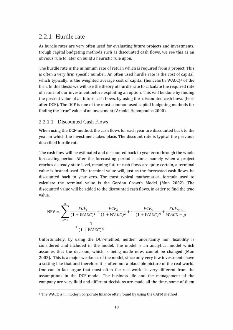
The cash flow will be estimated and discounted back to year zero through the whole

forecasting period. After the forecasting period is done, namely when a project

reaches a steady-state level, meaning future cash flows are quite certain, a terminal

value is instead used. The terminal value will, just as the forecasted cash flows, be

discounted back to year zero. The most typical mathematical formula used to

calculate the terminal value is the Gordon Growth Model (Mun 2002). The

discounted value will be added to the discounted cash flows, in order to find the true

value.

∑

( )

( )

( )

( )

Unfortunately, by using the DCF-method, neither uncertainty nor flexibility is

considered and included in the model. The model is an analytical model which

assumes that the decision, which is being made now, cannot be changed (Mun

2002). This is a major weakness of the model, since only very few investments have

a setting like that and therefore it is often not a plausible picture of the real world.

One can in fact argue that most often the real world is very different from the

assumptions in the DCF-model. The business life and the management of the

company are very fluid and different decisions are made all the time, some of them

3 The WACC is in modern corporate finance often found by using the CAPM method

11

are even changed from time to time. These new decisions and changed decisions will

naturally change the whole DCF-model, and make the former analysis of the true

value, by the best, useless.

These wrong assumptions make the discounted cash flow model very vulnerable

and that is a major weakness for the model. By using the above assumption, the

model can easily undervalue specific assets of the firm and does not incorporate the

value of different options and opportunities the company may have in the future.

Another of the DCF-model’s big weaknesses is the fact that it does not take

uncertainty into account. Of course some of the uncertainty is accounted for as a

negative object by the risk factor in the discount rate equivalent with the hurdle

rate. But there is a big uncertainty in the risk as well. In the real world the risk is

affected by many factors from the macro environment and is very likely to change

from year to year. In the DCF-model everything is locked and set to be stable after

the valuation.

The forecast in a DCF-model is essential. If the forecast is wrong so is the valuation.

It is very hard to predict the future. With that being said the discounted cash flow

model may be the most accurate method when applied carefully and correct. As

mentioned the methods demands careful valuation of the company’s future

strategies to estimate future cash flows. It must be assumed that the more detailed

this analysis is, all other things being equal, the more accurate the valuation of the

asset will be.

2.2.2 Profitability Index

Another often used capital budgeting method is the profitability index.

Sometimes companies have more than one project and limited capital resources to

projects, which forces the companies to choose between the different projects. One

way to choose between the projects is to use a profitability index (Berk, DeMarzo

2011). The profitability index is often used by practitioners to identify the optimal

combination of projects. The calculation is very simple and quite straight forward.

The value created is often replaced with the NPV as these two numbers is often

equivalent values. After calculating the profitability index for each individual

project, the numbers are placed in a table and ranked with the highest number first.

To select the most optimal combination of projects, the cumulative resources used

are calculated, and the projects which will maximize the value creation within the

resources are chosen.

There are some shortcomings of the profitability index. The algorithm only takes

one constraint into account. In the real world, companies are most often a subject to

12

multiples of constraint, such as employees, budgets, time etc. The algorithm is not

designed to make sure, that all of the resources are used. It is a very likely scenario

that even though there are not enough resources to adopt the next project in the

algorithm, other project with a lower profitability index is not demanding the same

amount of resources and it would then make sense to adopt those instead. This is a

fact, which the profitability index, do not take into account, and instead it is

stopping, when the first resource conflict occurs.

The profitability can be simplified. If it is assumed that the decision makers have

infinite money all projects which is greater or equal one ( )

should be invested in. Hence a profitability index of 1 will be the trigger value of

when to invest. As we are only interested in the individual project in this thesis and

comparison of other projects is not an issue, we can accept the assumption of

infinite money and use this simplification in the thesis.

2.3 Financial Options

The fundamental idea behind real options is based in the financial options, why it is

important to understand financial options to fully understand the logic behind real

options. In the following section the basic concepts of options and the most common

ways of valuating them will be introduced.

An option is a contractual agreement between two sides, giving the buyer the right,

but not the obligation, to buy or sell a specific asset to a predetermined price on or

before a given day. This gives the option holder the opportunity to exploit an upside,

and only have a limited downside. It is important to note that the rational investor

will only exercise the option, if the option is “in-the-money”. If the option does not

provide the option holder with a favorable price, the option will be left for

expiration and the maturity date.

Options can be divided into two types:

- A call option – the contract gives the option holder the right, but not the

obligation, to BUY an underlying asset at the predetermined price, in a given

time interval.

- A put option – the contract gives the option holder the right, but not the

obligation, to SELL an underlying asset at the predetermined price, in a given

time interval.

When one is looking at the exercise date, the option can be divided into further two

subgroups:

13

- An American option – an option where it is possible to exercise at any time

prior the maturity date

- A European option – an option which can only be exercised at the maturity

date.

Financial options are derivatives and just like other financial instruments,

companies are often using them to control and hedge their risks. The feature of the

option, which is different from other derivatives, where you are able to exploit an

upside and still have a limited downside, makes it an often used motivation tool as

well. If managers are given options to buy company shares, they are motivated to

work hard for the share price to rise, but unlike if they instead were given shares,

the managers would not fear taken chances, which could be a cost for them, as the

share price could drop. Just like other derivatives, options are also being used for

speculative purposes.

The price of an option is dependent on many different factors. The most important

and expressed is of course the difference between the spot and the exercise price,

but other factors such as the time to maturity is affecting the price as well (which

will be explained in the following paragraph).

The payoff of a call option can be expressed as the maximum value of the current

spot price of the underlying asset minus the exercise price and zero. Mathematically

it is noted as;

( )

Where is the exercise price and X is the spot price at the maturity. Through this

mathematical expression, it is also clear, that a call option will only be exercised as

long as , hence it can be bought at a favorable price.

For a put option the notation is opposite, the option will be exercised as long as the

strike price is higher than the current spot price, hence the underlying asset can be

sold at a favorable price . Mathematically the payoff can be noted as:

( )

2.3.1 Factors Affecting the Option Value

As mentioned earlier, many different variables are factors that affect the option

when determining the value. They are all affecting the value, either through the

containing information of the feature of the contract or by describing the

characteristics of the underlying asset and the market.

14

2.3.1.1 The Exercise Price

Of course the exercise price has a major effect on the price of the option. At the issue

date the option already have an intrinsic value, which is the maximum of zero and

the payoff of the option, if the option was to expire today. With a high intrinsic value

from the issue date (the spot price to exceed the exercise price), the possibility of

the spot price to be at higher level than the exercise price at the maturity date, is of

course higher, why a higher option price for a call option will follow.

In a put option it is of course opposite, an exercise price which is higher than the

spot price will raise the value. Just like the call option this indicates a higher chance

for a good payoff at the maturity.

2.3.1.2 The Maturity Date and Interest Rate

The effect of these two factors is to a great extent dependent of each other in a way,

in which they should be described together. Time value of money is of course a well-

known terminology and very well described in the economic literature, and is of

course also a factor in real options.

For a call option, time is a positive factor for the value of the option. Firstly, the

present value of the exercise price is reduced over time. Second, time gives a higher

chance for the positive spread, between the spot price and exercise price, to grow.

This is due to the fact that the volatility of the underlying asset is growing with the

square root of time.

The time value is however only appropriate to use in an American option, where the

option holder have the opportunity to exercise the price at any given price and time.

For European options, the time value does not have the same effect, since the option

holder does not have the flexibility to exercise the option, whenever it is appropriate

for the holder, but only at the maturity date.

To sum up – the risk free rate and the time, which combined is the time value of

money, is overall a good thing for a call option, since it decreases the value of the

price to be paid in the maturity time. For a call option, the decreased amount is the

value one has the right to sell its asset for. However time as itself is affecting it

positive because of the volatility, hence the risk of spot price of the asset to drop.

2.3.1.3 Volatility

Volatility is the biggest difference between classical capital budgeting method

theory and option theory. In the classical theory, volatility is seen as a risk and all

other thins equal risk is causing a higher discount rate, which is destroying value.

In option theory however, volatility is not seen as a risk, since the downside of the

volatility has been hedge away. The biggest lose one can have through an option, is

15

the price one have paid for the option. Instead volatility is seen as an opportunity,

why high volatility is creating value for the underlying asset.

2.3.1.4 Dividends/Return

Dividends are equity paid to the investors, why value is leaving the asset after an

outgoing cash flow like dividends. Another way to look at this, is through classical

capital budgeting methods, where the value of an investment is often found through

the future returns, as some of the returns are then gone, so is the value.

2.4 Real Options

With the fundamental ideas and logic behind options in mind, we can now turn to

the theoretical foundation of real options and thereby the foundation of the later

work in the thesis.

Probably the most important application of options in corporate finance lies in the

capital budgeting decision. Analogous with financial option a company that owns a

real option has the right, but not the obligation to make a potentially value creating

investment. The main difference between financial options and real options is that

the latter is often non-tradable assets, which are often illiquid. The price of a

financial option is determined by the market, whereas the price of a real option is

the costs of acquiring an opportunity. An acquirer of a real option has, in contrast to

an acquirer of a financial option, influence on the value of the option in the option’s

maturity, as the value is subject to good decisions. Therefore is competent

management crucial for the value of the real option (Kodukula, Papudesu 2006).

Valuing projects with traditional capital budgeting static and deterministic methods,

as explained earlier in this paper, do not consider the value of managerial flexibility.

Meaning that managers react or at least should react to changes in the economic

environment by adjusting the company’s plans and strategies. For instance

management may choose to abandon an unsuccessful project, scale up a successful

project, extend a successful project etc. The flexibility in management comes in

many different forms, whereas this paper will discuss only a part of those and those

different forms of flexibility may have considerable impact of the overall value of a

project (Koller et al. 2010b).

It is important to distinguish between managerial flexibility and uncertainty as it is

not the same. A project with a single management decision, whether or not to invest

can surely be properly valued using the discounted cash flow approach under

different scenarios. In contrast flexibility denotes choices between different plans

that managers may make when different events are revealed and, as already

mentioned, this flexibility can have substantial impact on the value of a given

16

project. With the above being said it is also important to mention that even though it

is important to distinguish between flexibility and uncertainty it is also very

important to know that the value of flexibility is very much related to the degree of

uncertainty and the room for managerial response. This means that when

uncertainty is highest and managers do have room to react on new information and

events the value of flexibility will be highest. In contrast if there is little uncertainty

managers are unlikely to receive new information that would have an impact on

future decisions, and also little room for managers to react, on this uncertainty the

value of flexibility will be lowest. This tells us much about when real option

valuation is important. Indeed it is therefore important to value such flexibility

especially when a project NPV is close to zero, meaning whether or not to go ahead

with the project is a difficult choice and sometimes management therefore go on

with a project for strategic reasons or gut feeling. To shed light on whether that is

beneficial for the company, a real option valuation approach can be used.

2.4.1 Drivers of Flexibility Value

To truly understand the value of real options it is important to be able to identify the

factors that drive the value of the assets flexibility.

Figure 2.1 – Drivers of Flexibility Value

Source: (Koller et al. 2010b)

The current value of the underlying asset is the present value of the expected future

cash flows from investing in a given project now. It is those future expected cash

Flexibility value

Time to expire

Cash flows (dividend

yield)

Uncertainty (volatility)

about present value

Value of the underlying

asset

Risk-free interest rate

Investment costs/

Exercise price

17

flows that are uncertain. If not and they instead were known with certainty there

would be no option value.

The longer maturity the option has, the higher is the flexibility value as the

management has the opportunity to learn about the future, which will strengthen

the decision making. The maturity is equivalent to the expiration date, which is

when the rights to a given project expire and therefore investment made after this

has a NPV of zero. In this thesis our later work is built upon a continuous-time

model, which is equivalent with an option that does not expire, meaning that the

company has the rights to this particular investment in perpetuity.

A higher risk free rate will increase the value of exposing the investment but will

also in turn reduce the net present value of the cash flow as a consequence of a

higher discount rate (Koller et al. 2010b).

When a company decides to invest in a project that they have the rights to the option

to is exercised. The investment cost of making the investment in the project is the

exercise price. Higher investment costs reduce the value of the flexibility. We

assume though, through the thesis, that this cost remains constant.

Greater uncertainty measured as volatility about the net present value of cash flows

will increase the value of the option, while reducing the net present value of the

underlying asset as the future is more uncertain. Higher net present value of the

underlying projects cash flow will also increase the value of the option. In other

words the higher the volatility, the higher the value of the option. This is also the

reason why an option in a stable business environment will be worth less compared

to a much more changing environment.

When a company is deferring a project it is the equivalent of not receiving the

dividend yield. That is the cost of deferring investing in a project, when the NPV has

become positive. The same happens if the company lose cash flow to competitors

due to exposing the investment.

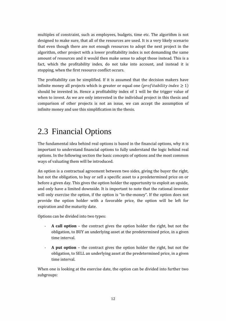
Below in Table 2.1 we provide an overview and summary of the effect on the option

value of a call option and the effect on a put option. Note that the effects from the

factors are in most cases just opposite from each other.

18

Table 2.1 – Factors Affecting the Option Value

Factor Effect on Call Value Effect on Put Value

Increase in Project Value (Underlying Asset) Increases Decrease

Increase in Investment Cost (Strike Price) Decreases Increases

Increase in Interest Rates Increases Decreases

Increase in time to expiration Increases Increases

Increase in Dividends Paid Decreases Increases

Increase in Volatility (Variance of Underlying Asset) Increases Increases

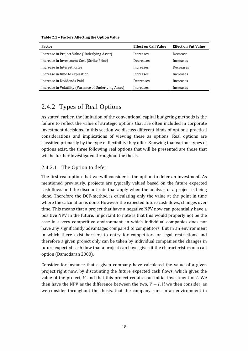
2.4.2 Types of Real Options

As stated earlier, the limitation of the conventional capital budgeting methods is the

failure to reflect the value of strategic options that are often included in corporate

investment decisions. In this section we discuss different kinds of options, practical

considerations and implications of viewing these as options. Real options are

classified primarily by the type of flexibility they offer. Knowing that various types of

options exist, the three following real options that will be presented are those that

will be further investigated throughout the thesis.

2.4.2.1 The Option to defer

The first real option that we will consider is the option to defer an investment. As

mentioned previously, projects are typically valued based on the future expected

cash flows and the discount rate that apply when the analysis of a project is being

done. Therefore the DCF-method is calculating only the value at the point in time

where the calculation is done. However the expected future cash flows, changes over

time. This means that a project that have a negative NPV now can potentially have a

positive NPV in the future. Important to note is that this would properly not be the

case in a very competitive environment, in which individual companies does not

have any significantly advantages compared to competitors. But in an environment

in which there exist barriers to entry for competitors or legal restrictions and

therefore a given project only can be taken by individual companies the changes in

future expected cash flow that a project can have, gives it the characteristics of a call

option (Damodaran 2000).

Consider for instance that a given company have calculated the value of a given

project right now, by discounting the future expected cash flows, which gives the

value of the project, and that this project requires an initial investment of . We

then have the NPV as the difference between the two, . If we then consider, as

we consider throughout the thesis, that the company runs in an environment in

19

which there exist barriers4, then even though the project right now may be negative

it might turn into a good project if the company decides to wait. The inputs needed

to value the option are those shown in Figure 2.1.

When viewing the option to defer a given project several interesting implications

appear. As mentioned even though that a given project may have a negative NPV and

therefore a company reject the project, the rights to this project is not necessary

worthless. Secondly, even though the given project has a positive NPV this does not

necessarily have to be accepted and thereby invested. This is likely to happen if the

company holds the right to a given investment for a long time, which will be the case

in our later, rather simple continuous-time model. To illustrate this, we can assume

that a company holds a patent for producing some special item and that building a

plant for producing this product evolves a positive NPV right now. However there is

currently huge development within the production methods on this type of product

and it seems that it will become significantly cheaper to produce this kind of product

in the future. Therefore the company has incitement to wait and perhaps increase

the cash flow that will flow to the company from the project in the future. This is

especially the case when a company is making an irreversible investment, which is

the case throughout this thesis. The reason for this is that if management cannot

disinvest and recover the initial expenditures if the cash flows are worse than

expected the investment timing decision should be taken with caution and therefore

the project should be deferred until the project or the cash flows gives a premium

sufficiently over the NPV (Smit, Trigeorgis 2004). Of course this must be weighed

against the foregone dividends yields/cash flow that would have come from

investing now. Third, viewing a given project as an option can make factors,

included in a conventional NPV analysis, that normally would make investment in a

given project less attractive actually can make the rights to the project worth more

(Damodaran 2000). For instance the uncertainty about future cash flow would

heighten the discount rate in a normal NPV but when viewing the project as an

option, volatility would make the option worth more.

2.4.2.2 The Option to Expand

Some companies invest in projects which have a negative NPV because the

companies then get access to other projects that then have positive NPV’s. It can be

argued then that taking the first investment should be viewed as an option that

permits the company to make other projects. To estimate the value of such an option

this option can be viewed just as the above option to defer. Moreover options to

expand have often no specific expiration date, which means that they often have

characteristics of a continuous-time model or indefinite lives.

4 meaning that the company has wholly rights to this project for the next years and that the cash flows might change over time either because of the discount rate or change in cash flows

20

The option to expand is often seen used by many companies, for instance investing

in projects with negative NPV’s that makes the company capable and provide the

opportunity of opening and sell their products in new markets. As was the case with

the option to defer, it is also the option to expand is often more valuable in business

in which the volatility is high compared to those with lower volatility.

2.4.2.3 The Option to Abandon

The last of the three options that will be presented in this thesis is the option to

abandon a project if the cash flow does not equal the expectations. Compared to the

above two options this option has the characteristics of a put option.

A typical abandonment option could be in the situation where a company has

hedged its investment, with a contract, allowing the company to sell some of its

investments at a predetermined and contracted price. It could be in the example of a

company has invested in a joint venture with a partner. This hedge will allow the

company to obtain a scrap value even though the investments have been very asset

specific and in a normal situation would have had a scrap value of zero. We note

further that when a given firm is dealing with an option to abandon, the

considerations are completely opposite to the ones of a call option. Now a given

firms do not want to be sure of the cash flow to be significant over the investment,

but significant under the scrap value instead. The firm cannot be sure of how it will

look in the future.

Throughout the thesis we assume rather unrealistically that the abandonment value

can be clearly identified before making the investment and that it is not changed

during the life time of the project. We note that this is only the case in some very

specific cases and there almost always will be some noise around this parameter.

2.4.3 Valuing Real Options

With the starting point in the article from McDonald and Siegel (MacDonald 1986)

Dixit and Pindyck (Dixit, Pindyck 1994) provide two techniques that are able to

handle the valuation of investment options, respectively the dynamic programming

(hereafter DP) and contingent claims analysis (hereafter CCA). The two methods are

very close related and should in many applications lead to identical results however

they are different in their underlying assumptions about financial markets and the

discount rates that the firms use to value future cash flow. Both methods can be

used to solve investment problem, which are perpetual, analytically.

2.4.3.1 Dynamic Programming and Contingent Claims Analysis

Dynamic programming breaks a whole sequence of decisions into just two

components, namely a component, which should reflect the value of the immediate

decision and a component which should reflect all subsequent decisions, a value

21

function. If the company’s decision horizon is finite the last decision can be found by

standard optimization methods. The solution of that gives the value function, which

should be used to the second last decision and in that sense one can work

backwards until the first decision is met. An infinite is simplified by the problem’s

recursive structure, meaning that every decision leads to a new problem, which is

exactly the same as the original problem.

CCA is based on the ideas from financial theory and especially the assumption of an

efficient market. The idea behind CCA is that the firm or individual owns the right to

an investment opportunity, or to a stream of operating profits from a project, and

we are assuming that this asset can be traded in the market. Even if the exact assets

or investment project is not directly traded in the market it is possible to compute

an implicit value for it by relating it to other assets that are traded. This means that

the method requires that it is possible to make a portfolio of traded assets, which

will exactly replicate the pattern and returns from the investment project at every

possible outcome. The method relies on market equilibrium, which means that

arbitrage opportunities immediately will disappear. An alternative and similar

methods to the same result as by the replicating portfolio methods is to construct a

portfolio, which consist of the company’s investment option and units of a short

position in that underlying asset or a portfolio, , which is perfect correlated with

the project. is then chosen in a way such that the portfolio becomes risk-free and

the return from this portfolio is then equal to the risk-free return.

The investment problems that we will be considering in this thesis will be in line

with the paper from (MacDonald 1986) solved in continuous time, which is often

done using partial differential equations (hereafter PDE). By using either DP or CCA

it is possible to derive a PDE that the investment option must satisfy, which is used

to find a problem solution. According to Dixit and Pindyck (1994) the main

difference between the two methods in relation to their PDE’s is their different

assumptions about the financial markets and the discount rate that the company is

using to assess future cash flows. By DP the discount rate is specified exogenous as a

part of the object function. The problem here is that it is not obvious what the

discount rate should be and where it should be collected. One could argue that it is

somewhat arbitrary. By CCA the required rate of return on the assets is calculated

from the equilibrium in the capital markets and it is only the risk-free rate that is

given exogenous. Therefore the CCA somewhat handle the discount rate in a better

way, compared to DP. In contrast the CCA method instead requires that there exists

a complete or at least sufficiently market for assets so that the return on the given

asset can be replicated exactly, whether it is on a single asset or a portfolio of assets.

This is a quite restrictive assumption as the assets should be perfectly correlated

such that every outcome of a process is replicated by the other and as discussed in

(Borison 2005) the primary difficulty with this approach is the contention that a

traded replicating portfolio of financial assets exist for a typical corporate

investment in real assets.. DP does not have such an assumption. If risk cannot be

22

traded in the market, the object function can reflect the decision maker’s objective

assessment of the risk.

2.4.3.2 Continuous-time Models

In this section we introduce a series of concepts, models and definitions within the

discipline of real option valuation, which will be used throughout the thesis. We

start by describing a basic continuous-time model, where the investment is

irreversible, meaning that when this investment has been taken the cost of that

investment turn into a sunk cost and cannot in any way be redone. This is the basic

model that will be used to validate both the option to defer, the option to expand

and the option to abandon throughout the thesis.

By using the continuous-time model we are working with a perpetual option, which

is very important to notice, since it is a big difference to financial option which often

has an expiration date.

When a company exercises an option, the company becomes exposed to volatility.

Thinking in terms of a financial option with an expiration date, and with no payoff,

such as dividends, during the possible exercise period, we would wait to take the

decision whether of exercising or not, to the last day. Taking the decision earlier on

will not give any advantages but only make you vulnerable towards volatility. By

waiting instead, you will only have the upside of the investment and a very limited

downside (by not exercising the option you will lose the investment in the option).

In a perpetual real option it is an entirely different scenario. At first, for the option to

have any value at all, you must have the intention of making use of it, at a certain

point, logical enough. Secondly, for an investment to have value it must deliver some

kind of payoff(s). In most financial cases the payoff will be a cash flow, which will be

used during this thesis as well. By waiting to invest, and instead using an option to

defer, you will not receive any payoff and cash flows will therefore be lost. By

waiting you will not be vulnerable to lower cash flow than expected and risk making

an overinvestment (an investment with a negative NPV).

The question therefore is, when it is best to make the investment. A calculation

should therefore contain the tradeoff between not missing too much cash flow and

in the same time, not to be threatened by a big downside and make bad investment.

We will examine the theoretical best estimate of when it is the best point to exercise

the option and when to wait and not use the value. Before examine the answer, we

note that it will probably be at a point where the cash flow are at such a high point,

that even though they will drop, the NPV of the investment will still be positive. This

point is of cause different from case to case and a subject to the discount rate,

volatility of the investment and the risk free rate. We next consider the basic model.

23

2.4.3.3 A fundamental Model

In this section a fundamental model to real option valuation will be introduced. In

this basic model the problem for a given company is both if and when it should

invest in a known and fixed cost for a given project, .

Dixit (1992) argues that to be able to calculate the value of waiting, we need to

assume that three assumptions are satisfied. The first assumption is that after

making the investment it cannot be undone; hence the investment is irreversible

and will be treated as a sunk cost. The second assumption is that the economic

environment is uncertain and it can only be guessed upon how the economic factors

will develop over time. At last, we are assuming that the investment opportunity is

not a now or never decision, we will be able to make the investment on a later stage.

In normal capital budgeting methods we will invest in projects if the discounted

revenues will exceed the investment and is treated as a now or never investment.

When we introduce uncertainty and flexibility to our considerations, we can use

option theory, to calculate a result, which in theory is superior. The reasoning

behind this is that by the flexibility of waiting to invest we are in a position of, in

which we can use to limit our downside. We can simply wait and see how the

economy is developing, and when the revenue is reaching a certain value the profit

is superior to the risk. This certain level of revenue is called the “trigger value”. The

intuition of the trigger value and the calculation of it will be described in a later

section of this thesis.

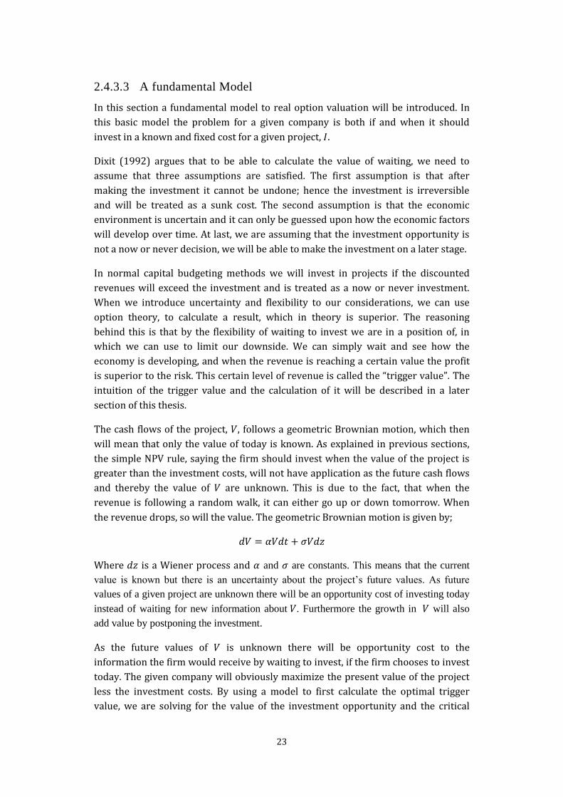
The cash flows of the project, , follows a geometric Brownian motion, which then

will mean that only the value of today is known. As explained in previous sections,

the simple NPV rule, saying the firm should invest when the value of the project is

greater than the investment costs, will not have application as the future cash flows

and thereby the value of are unknown. This is due to the fact, that when the

revenue is following a random walk, it can either go up or down tomorrow. When

the revenue drops, so will the value. The geometric Brownian motion is given by;

Where is a Wiener process and and are constants. This means that the current

value is known but there is an uncertainty about the project’s future values. As future

values of a given project are unknown there will be an opportunity cost of investing today

instead of waiting for new information about . Furthermore the growth in will also

add value by postponing the investment.

As the future values of is unknown there will be opportunity cost to the

information the firm would receive by waiting to invest, if the firm chooses to invest

today. The given company will obviously maximize the present value of the project

less the investment costs. By using a model to first calculate the optimal trigger

value, we are solving for the value of the investment opportunity and the critical

24

value or trigger value (hereafter synonyms)of , , which is the value where it

would be optimal for the given company to make use of their option to invest in the

given project.

The optimal investment rule, which is showed below, is to invest when is at least

as high as a critical value, which exceed . The company wishes of course to

maximize the expected net present value of the project less the investment costs.

2.4.3.3.1 Solution by contingent claims analysis

In this section we derive a solution by contingent claims analysis. The use of

contingent claims analysis requires, as mentioned earlier, one important assumption

– that stochastic change in can be replicated by existing assets in the economy.

Especially the capital markets must be sufficiently complete, meaning that at least in

principle it should be possible to find an asset or construct a dynamic portfolio of assets,

which price is perfectly correlated with. It can surely be discussed whether it is possible

to construct a portfolio that is perfectly correlated with. For now we will although assume

that the assumptions stated above holds, that the uncertainty over future values of can

be replicated by existing assets and we can therefore determine the investment rule that

maximizes the firm’s market value without any assumptions about risk preferences or

discount rates.

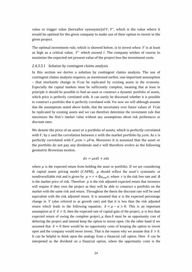
We denote the price of an asset or a portfolio of assets, which is perfectly correlated

with , by and the correlation between with the market portfolio by . As is

perfectly correlated with , . Moreover it is assumed that the asset or

the portfolio do not pay any dividends and will therefore evolve as the following

geometric Brownian motion.

where is the expected return from holding the asset or portfolio. If we are considering

th capital assets pricing model (CAPM), should reflect the asset’s systematic or

nondiversifiable risk and is given by , where is the risk free rate and

is the market price of risk. Therefore is the risk adjusted expected return that investors

will require if they own the project as they will be able to construct a portfolio on the

market with the same risk and return. Throughout the thesis the discount rate will be used

equivalent with the risk adjusted return. It is assumed that is the expected percentage

change in (also referred to as growth rate) and that it is less than the risk adjusted

return which leads to the following equation; . This is an important

assumption as if , then the expected rate of capital gain of the project, is less than

expected return of owing the complete project, then must be an opportunity cost of

deferring the project and instead keep the option to invest open. On the other hand if we

assumed that there would be no opportunity costs of keeping the option to invest

open and the company would never invest. That is the reason why we assume that .

It can be helpful to think upon the analogy from a financial call option. Here can be

interpreted as the dividend on a financial option, where the opportunity costs is the

25

dividends the company gives up by holding the option instead of the stock (Dixit,

Pindyck 1994).

Obtaining a solution by using the contingent claims methods, ( ) and in the

model is found by constructing a risk free portfolio, thereafter determine the

expected rate of return of that portfolio and equating that expected rate of return to

the risk free rate of interest. The risk free portfolio is constructed by holding the

option of investing, go short in units of the project (or the asset or portfolio that

is perfectly correlated with ). This portfolio would be dynamic however over each

short interval of length we hold constant. The value of the portfolio is

An investor which is long in the project will require the risk adjusted return

which equals the capital gain plus the dividend stream . The short position in

units will therefore require paying out . The total return from holding the

portfolio over a short time interval is therefore

is found by Itôs lemma. The derivation of that can be found in Appendix 1

( ) ( ) ( )

The above equation is a differential equation that ( ) must satisfy. In addition

( ) must also satisfy the following three boundary conditions.

( )

It is seen from the stochastic process for that if goes to zero, it will stay at zero.

Meaning that if the value of the project once turned to zero the opportunity to invest

will be of no value.

( )

The condition above is called the value matching condition as it says that upon

investment the firm will receive a net payoff. In other words, it says that the

unknown function of ( ) equals the known payoff by exercising the option. The

critical value, where it is optimal for the company to exercise its option to invest

in a given project, the value of that option must be equal to the yield that the

company will get by exercising, which is as given in the above equation, is the value

of the project less the investment costs..

This condition has also another very useful interpretation. If the equation instead is

written as ( ) it can be seen that it will first be optimal for the company

to exercise the option to invest at the critical value, where the value of the project

26

equals the full cost, which is the direct cost plus the opportunity costs ( ) there

is when the company give up the opportunity to invest.

( )

This condition is called the smooth-pasting condition as it requires that not only the

values but also the slopes of the two functions equals by the boundary. The one on

the right hand side is the exercise value differentiated with relation to .

This condition together with the value matching condition should both be fulfilled in

order to secure that is the optimal point to exercise the option.

To satisfy the first boundary condition, the solution must take the form

( )

Where is a constant and is a known constant which values are given by the

parameters , and of the differential equation. The last two boundary conditions

can be used to solve for the last two remaining unknowns, the constant and the

critical value .

( ) ( )

( )

The three above equations gives the value of the investment opportunity and the

optimal investment rule, the critical value at which it is optimal to invest. There

are some restrictions attached to these formulas as well:

The quadratic equation for the exponent β1 is given by:

(

( )

) √(

( )

)

With the CCA solution method we can solve the investment problem by assuming

the restrictive assumption that the assets or a portfolio of assets are perfectly

correlated. If this assumption did not hold we should in order to solve the

investment problem solve the problem by DP but then we would have to subjective

find an assumed discount rate.

27

The value of the option to defer is calculated by:

( ) ( ) (

)

2.4.3.4 Abandonment Option

The abandonment option is in contrast to the previous options, not a call option but

a put option. As explained previously in the thesis the call option is designed to

exploit an eventual upside. In contrast the put option is designed to limit the

downside.

The difference between a put and call option, makes the root β1 not applicable.

Therefore we need to use the root β2 instead

(

( )

) √(

( )

)

Note that, the major difference between β1 and β2 is the fact that the two terms are

subtracted in β2 instead of being added as they are in β1 (Dixit, Pindyck 1994).

In the call option the value have to reach a certain point in order to exploit the

option at the best possible time, but as we here have a put option, which is designed

to limit the downside and not exploit the upside, the value have to drop to a certain

amount, before exploiting the abandonment option. The optimal trigger value for the

abandonment option is given by:

( )

The new factor S is denoting the fixed price one can sell the project/asset for. The

formula is very similar to the formula that has been used for the call option, with one

very significantly change; has been replaced with . The purpose of the formula

is to find the value, where it will be appropriate for a given company to exploit the

option to stop the operations and redeem the scrap value, as the whole point of real

option is the idea to exploit the volatility of the investment.

In this scenario even though the operations are unprofitable, the optimal solution is

not always to stop them. The cash flows of the operations are of course volatile and

through time the deficit and lacking revenue can turn into a positive and “good”

return on the investment. If a given company did choose to shut down the

operations after years with deficit, it can be very costly for them to start up the

operations again. This can be a question of hiring new employees again, building

new factories or setting up supply chains.

28

From this belief, the formula is designed to find a value, where the best economical

solution for a given company will be to stop the operations when the volatility is

considered. And by introducing an abandonment (put) option, where a company has

either secured a scrap value either through contract or by other means, the company

will be able to raise that level a limit their downside. This will intuitively make the

companies use a lower hurdle rate, as they are not risking the same amount.

2.4.3.5 Expansion Option

The expansion option is, just like the option to defer, a call option. The fundamental

idea behind this option is to expand the project to ensure maximization of the

raising cash flow. The option will typically appear when a company has made a small

investment in a foreign market for learning, watching or a third reason. An

expansion will typically demand further investment and by investing more in the

project, the project will become more vulnerable towards falling cash flows as the

breakeven point will be raised. To be sure of making a good investment, and not get

too exposed towards volatile cash flows, intuitively the trigger value will have to

reach a higher point, than it would at an option to defer, which is caused by the

bigger investment, which is made.

For the option to exist, the investment cost should be the same amount, no matter

when one decides to take strike and exploit the option.

The optimal trigger value for the expansion option:

( )

The new factor ‘e’ is an extra percentage of capacity the company will receive when

the company invest . It denotes the investment amount and is fixed. So when the

expansion is done, a given company will invest a fixed amount, , and receive

additional , with denoting the underlying asset (Smit, Trigeorgis 2004).

The larger , the more a given company will get for the extra invested amount, and

the trigger value will therefore go towards zero as goes to eternity. The purpose of

this formula is to find the right time to expand the operations, when volatility is

taken into account. Even though the demand is reaching a level, where the supply

cannot keep up it is not always the right decision to expand its operations right

away. The cash flow is still volatile and will fluctuate over time, why it can easily

drop to a level where an expansion is not appropriate. By calculating the optimal

trigger value and talking the volatility into account, one will find the point where an

expansion of the operations can be justified over time.

Just like in the option to wait, the condition value of an expansion option can be

calculated very simple, with the right numbers available.

29

The optimal condition for the value of an expansion option is given by:

( )

With being a nomination for the size of the expansion option

The value of the expansion option;

( ) ( ) (

)

2.4.4 Discussion of the Characteristics of the Optimal

Investment Rule

This section discusses the optimal investment rule in relations to the different

parameters used in the model. Moreover the section will provide some numerical

solutions to the optimal investment rule in order to explain and better understand

the model. It should be clear from this section what will happen if some of the

parameters change in the obtained equations and what the effect to the model will

be. It will also be seen from the below illustrations that the results are qualitatively

the same as those which will appear from standard option pricing models of

financial options (Dixit, Pindyck 1994).

As we have mentioned previously a given firms option to invest in a project can be

seen equivalent with an infinite call option on a dividend paying stock in which is

the stock price and is the proportional dividend rate and is the exercise price. To

help illustrate how the optimal investment rule depends on the various parameters

we have in the following randomly chosen some values to the different parameters.

These will appear from the different figures below. It is important to notice that in

the below calculations behind the figures we use the term , which is the difference

between the discount rate, and the growth rate, . It is not necessary to know the

values of both and but only the difference between them, which is as

mentioned before the payout rate on a given project. If nothing else is stated about

the NPV we have taken the assumption in all the below figures that the value of the

project is set equal to the investment so that the NPV is zero. The reason to this is to

keep our illustrations as simple as possible. We now turn to the illustration of the

different parameters effect on both the value of investment option and the trigger

value meaning what the value of following the optimal investment rule is and when

to follow it – when it is optimal to invest.

2.4.4.1 Characteristics of the Option to Defer

The first option we consider is the simple option to defer the investment. In the

below Figure 2.2 the option value as a function of the value of a project is shown for

different values of the volatility, . The point where the different set of parameters

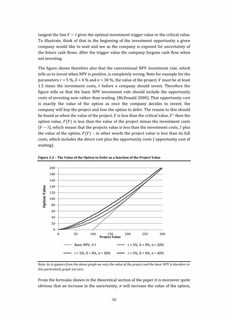
30

tangent the line gives the optimal investment trigger value or the critical value.

To illustrate, think of that in the beginning of the investment opportunity a given

company would like to wait and see as the company is exposed for uncertainty of

the future cash flows. After the trigger value the company forgone cash flow when

not investing.

The figure shows therefore also that the conventional NPV investment rule, which

tells us to invest when NPV is positive, is completely wrong. Note for example for the

parameters = 5 %, = 4 % and = 30 %, the value of the project, must be at least

1.5 times the investment costs, before a company should invest. Therefore the

figure tells us that the basic NPV investment rule should include the opportunity

costs of investing now rather than waiting. (McDonald 2000). That opportunity cost

is exactly the value of the option as once the company decides to invest; the

company will buy the project and lose the option to defer. The reason to this should

be found as when the value of the project, is less than the critical value, then the

option value, ( ) is less than the value of the project minus the investment costs

( ), which means that the projects value is less than the investment costs, plus

the value of the option, ( ) – in other words the project value is less than its full

costs, which includes the direct cost plus the opportunity costs ( opportunity cost of

waiting).

Figure 2.2 – The Value of the Option to Defer as a function of the Project Value

Note: As it appears from the above graph we vary the value of the project and the basic NPV is therefore in

this particularly graph not zero.

From the formulas shown in the theoretical section of the paper it is moreover quite

obvious that an increase in the uncertainty, will increase the value of the option,

0

20

40

60

80

100

120

140

160

180

200

0 50 100 150 200 250 300

Op

tio

n V

alu

e

Project Value

Basic NPV, V-I r = 5%, δ = 4%, σ = 20%

r = 5%, δ = 4%, σ = 30% r = 5%, δ = 4%, σ = 40%

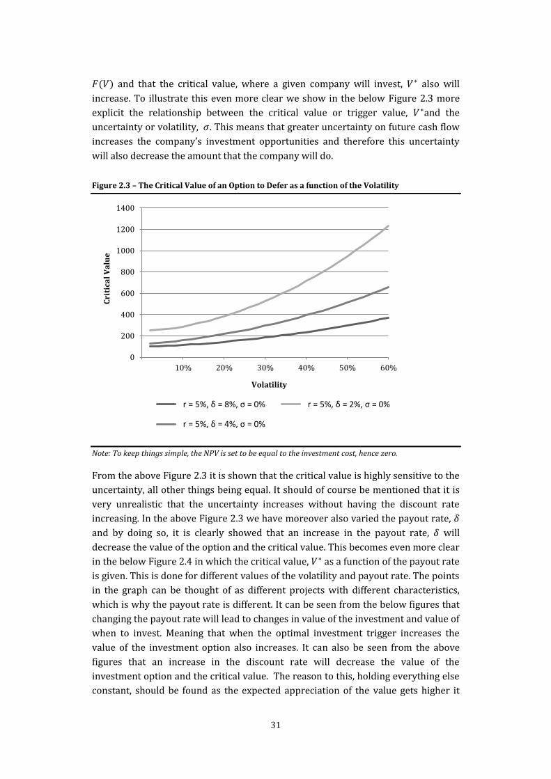
31

( ) and that the critical value, where a given company will invest, also will

increase. To illustrate this even more clear we show in the below Figure 2.3 more

explicit the relationship between the critical value or trigger value, and the

uncertainty or volatility, . This means that greater uncertainty on future cash flow

increases the company’s investment opportunities and therefore this uncertainty

will also decrease the amount that the company will do.

Figure 2.3 – The Critical Value of an Option to Defer as a function of the Volatility

Note: To keep things simple, the NPV is set to be equal to the investment cost, hence zero.

From the above Figure 2.3 it is shown that the critical value is highly sensitive to the

uncertainty, all other things being equal. It should of course be mentioned that it is

very unrealistic that the uncertainty increases without having the discount rate

increasing. In the above Figure 2.3 we have moreover also varied the payout rate,

and by doing so, it is clearly showed that an increase in the payout rate, will

decrease the value of the option and the critical value. This becomes even more clear

in the below Figure 2.4 in which the critical value, as a function of the payout rate

is given. This is done for different values of the volatility and payout rate. The points

in the graph can be thought of as different projects with different characteristics,

which is why the payout rate is different. It can be seen from the below figures that

changing the payout rate will lead to changes in value of the investment and value of

when to invest. Meaning that when the optimal investment trigger increases the

value of the investment option also increases. It can also be seen from the above

figures that an increase in the discount rate will decrease the value of the

investment option and the critical value. The reason to this, holding everything else

constant, should be found as the expected appreciation of the value gets higher it

0

200

400

600

800

1000

1200

1400

10% 20% 30% 40% 50% 60%

Cri

tica

l V

alu

e

Volatility

r = 5%, δ = 8%, σ = 0% r = 5%, δ = 2%, σ = 0%

r = 5%, δ = 4%, σ = 0%

32

will become more expensive to wait compared to investing now. The same is

happening if the discount rate is being held constant while expected growth rate of

the value of the project, falls, then the expected appreciation in the value of the

option to invest and acquire the value of the project, falls.

Figure 2.4 – The Critical Value of an Option to Defer as a function of the Payout Rate

Note: The value of the project is set to be equal to the investment cost, hence the NPV is zero.

To see the effect a change in the risk free rate we show in Figure 2.5 below the

critical value as a function of the risk free rate for different set of parameters. We see

that an increase in the risk free rate will have an increasing effect on the option

value as a given company will refrain from investing and therefore fewer options

will be exercised due to a higher rate will increase the value of the option to invest

and therefore also the opportunity costs of investing now.

0

200

400

600

800

1.000

1.200

1.400

1.600

0% 5% 10% 15% 20%

Cri

tica

l V

alu

e

Payout Rate

r = 5%, σ = 20% r = 5%, σ = 30%

r = 0%, δ = 8%, σ = 30%

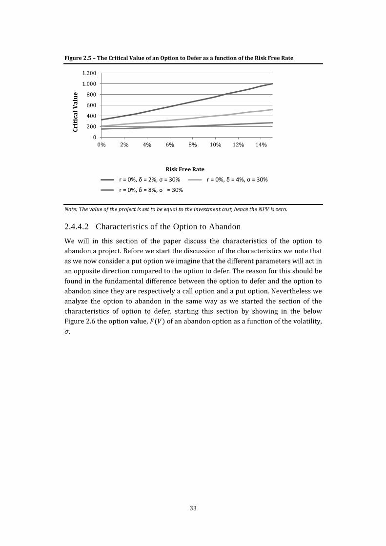
33

Figure 2.5 – The Critical Value of an Option to Defer as a function of the Risk Free Rate

Note: The value of the project is set to be equal to the investment cost, hence the NPV is zero.

2.4.4.2 Characteristics of the Option to Abandon

We will in this section of the paper discuss the characteristics of the option to

abandon a project. Before we start the discussion of the characteristics we note that

as we now consider a put option we imagine that the different parameters will act in

an opposite direction compared to the option to defer. The reason for this should be

found in the fundamental difference between the option to defer and the option to

abandon since they are respectively a call option and a put option. Nevertheless we

analyze the option to abandon in the same way as we started the section of the

characteristics of option to defer, starting this section by showing in the below

Figure 2.6 the option value, ( ) of an abandon option as a function of the volatility,

.

0

200

400

600

800

1.000

1.200

0% 2% 4% 6% 8% 10% 12% 14%

Cri

tica

l V

alu

e

Risk Free Rate

r = 0%, δ = 2%, σ = 30% r = 0%, δ = 4%, σ = 30%

r = 0%, δ = 8%, σ = 30%

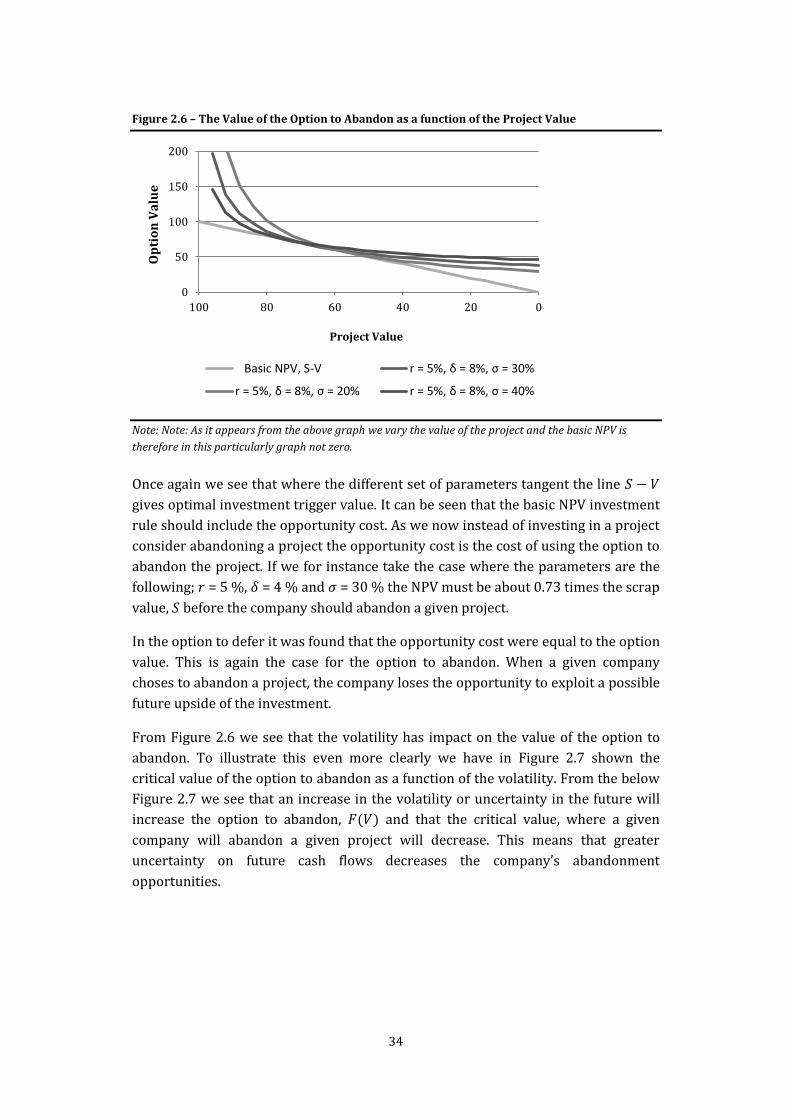
34

Figure 2.6 – The Value of the Option to Abandon as a function of the Project Value

Note: Note: As it appears from the above graph we vary the value of the project and the basic NPV is

therefore in this particularly graph not zero.

Once again we see that where the different set of parameters tangent the line

gives optimal investment trigger value. It can be seen that the basic NPV investment

rule should include the opportunity cost. As we now instead of investing in a project

consider abandoning a project the opportunity cost is the cost of using the option to

abandon the project. If we for instance take the case where the parameters are the

following; = 5 %, = 4 % and = 30 % the NPV must be about 0.73 times the scrap

value, before the company should abandon a given project.

In the option to defer it was found that the opportunity cost were equal to the option

value. This is again the case for the option to abandon. When a given company

choses to abandon a project, the company loses the opportunity to exploit a possible

future upside of the investment.

From Figure 2.6 we see that the volatility has impact on the value of the option to

abandon. To illustrate this even more clearly we have in Figure 2.7 shown the

critical value of the option to abandon as a function of the volatility. From the below

Figure 2.7 we see that an increase in the volatility or uncertainty in the future will

increase the option to abandon, ( ) and that the critical value, where a given

company will abandon a given project will decrease. This means that greater

uncertainty on future cash flows decreases the company’s abandonment

opportunities.

0

50

100

150

200

100 80 60 40 20 0

Op

tio

n V

alu

e

Project Value

Basic NPV, S-V r = 5%, δ = 8%, σ = 30%

r = 5%, δ = 8%, σ = 20% r = 5%, δ = 8%, σ = 40%

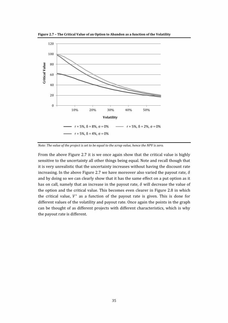
35

Figure 2.7 – The Critical Value of an Option to Abandon as a function of the Volatility

Note: The value of the project is set to be equal to the scrap value, hence the NPV is zero.

From the above Figure 2.7 it is we once again show that the critical value is highly

sensitive to the uncertainty all other things being equal. Note and recall though that

it is very unrealistic that the uncertainty increases without having the discount rate

increasing. In the above Figure 2.7 we have moreover also varied the payout rate,

and by doing so we can clearly show that it has the same effect on a put option as it

has on call, namely that an increase in the payout rate, will decrease the value of

the option and the critical value. This becomes even clearer in Figure 2.8 in which

the critical value, as a function of the payout rate is given. This is done for

different values of the volatility and payout rate. Once again the points in the graph

can be thought of as different projects with different characteristics, which is why

the payout rate is different.

0

20

40

60

80

100

120

10% 20% 30% 40% 50%

Cri

tica

l V

alu

e

Volatility

r = 5%, δ = 8%, σ = 0% r = 5%, δ = 2%, σ = 0%

r = 5%, δ = 4%, σ = 0%

36

Figure 2.8 – The Critical Value of an Option to Defer as a function of the Payout Rate

Note: The value of the project is set to be equal to the scrap value, hence the NPV is zero.

It can be seen from the above Figure 2.8 that changing the payout rate will lead to

changes in value of the abandonment option and value of when to abandon. Meaning

that, as we have discussed earlier when the optimal investment trigger decreases

the value of the investment option increases. It can also be seen from the above

figures that an increase in the discount rate will decrease the value of the critical

value, which in turn will make the abandonment option worth more. The reason to

this, holding everything else constant, should be found in the fact that when the

value of all the future incomes rises, then it will be more attractive to “stay” in the

investment, compared to abandon the investment.

To see if the effect on a change in the risk free rate is the same as in the call option

we show in Figure 2.5 below the critical value as a function of the risk free rate for

different set of parameters. We see that an increase in the risk free rate will have an

decreasing effect on the option value and more options will therefore be exercised

due to a higher rate will decrease the value of the option to abandon and therefore

also the opportunity costs by abandoning now.

0

10

20

30

40

50

60

70

80

0% 5% 10% 15% 20% 25% 30%

Cri

tica

l V

alu

e

Payout Ratio

r = 5%, σ = 20% r = 5%, σ = 30%

r = 0%, δ = 8%, σ = 30%

37

Figure 2.9 – The Critical Value of an Option to Defer as a function of the Risk Free Rate

Note: The value of the project is set to be equal to the scrap value, hence the NPV is zero.

2.4.4.3 Characteristics of the Option to Expansion

Having discussed the characteristics of the option to defer an investment in a project

and the option to abandon a project we now turn to the characteristics of the option

to expand an investment. But as the option to expand as we have explained

previously is a call option in line with the option to defer the characteristics will be

the same of the two. The only difference between the two call options is the

parameter , which is an extra percentage capacity a given company will receive

when it invest, . This parameter will depending either on the size of raise or

lower the trigger value and therefore also the option value.

Above we have shown different illustrations on how the different parameters in the

optimal investment rule affect the calculation. By doing so, we have provided a

thorough understanding of the investment rule, which we then can develop further

on. It should although at this point be noted that it is very careful to interpret the

rule as we have done above as we vary one parameter and all others being equal.

This is unlikely to be the case in practice as the different parameters seldom are

independent from each other. For instance, as (McDonald 2000) note that an

increase in the risk free rate, is likely to effect in an increase in the risk-adjusted

expected return, , which we have discussed in earlier sections of the theoretical

foundation. And if the drift rate, is constant then an increase in the risk-adjusted

expected return implies an increase in the payout rate, . Moreover an increase in

the volatility or uncertainty will also most likely result in an increase in the risk-

adjusted return, which then again implies an increase in the payout rate.

0

10

20

30

40

50

60

70

80

0% 5% 10% 15%

Cri

tica

l V

alu

e

Risk Free Rate

r = 0%, δ = 2%, σ = 30% r = 0%, δ = 4%, σ = 30%

r = 0%, δ = 8%, σ = 30%

38

2.4.5 Measuring the Cost of Non-Optimal Investment

In real option valuation we are interested in finding the optimal investment decision

rule, the before mentioned investment trigger value and also the value of that

investment decision rule, namely the value of the investment option. As we

previously have explained we are able to approximate the optimal investment

decision rules into suboptimal decision rules as for instance the hurdle rate, or

profitability index. The main question of this paper is to investigate how such

approximations perform and thereby if such rules are acceptable for practical

purposes. This section will discuss the effect on the value of the investment option if

the optimal decision rule is not being used.

In the below figure we show different non-optimal investment policies, which gives

us an overview of how the investment option varies when following non optimal

investment policies. The first option we will investigate is the option to defer the

investment. As mentioned before in this paper an exercise of the option will take

place if the net present value of the investment reaches a certain level. To analyse

the effect of deferment we have in the below figure, in line with McDonald

(McDonald 2000) varied this value of the investment named the trigger value as it

triggers investment, when the value of the project reaches a certain level.

In the below figure we vary the investment trigger value or the critical value,

from 100 – 1000 assuming a risk free rate of 5 % and the investment cost of 100.

The maximum value of each line, with different assumptions, reflects the optimal

investment trigger.

Figure 2.10 – Non-optimal investment triggers, option to defer

0

5

10

15

20

25

30

35

10

0

15

0

20

0

25

0

30

0

35

0

40

0

45

0

50

0

55

0

60

0

65

0

70

0

75

0

80

0

85

0

90

0

95

0

1.0

00

Op

tio

n V

alu

e

Trigger Value

r = 5%, ρ = 12%, σ = 30% r = 5%, ρ = 5%, σ = 30%

r = 5%, ρ = 20%, σ = 30% r = 5%, ρ = 12%, σ = 40%

39

The curve is quite steep before reaching the optimal trigger point, hence

underestimation of the trigger point is destroying the option value. This cost occurs

as an underestimation will make us more vulnerable towards the volatility and a

possible decrease in the cash flow.

After the curve has passed the optimal trigger value, the option value will fall again.

This is due to the cost of entering the investment too late and the cost of lost cash

flows

It is obvious from the figure above that, first of all it is worst to invest when the

investment value is equal to the value of the project, hence NPV is zero. It can also be

seen that the investment option values are not normal distributed meaning that the

loss is asymmetric and that it is therefore seems better to wait too long than invest

too early. Moreover we can conclude that the optimal investment trigger of course

has much to say about the investment option value but that many investment

triggers will give roughly the same or at least close the same results as the optimal

investment trigger. From Figure 2.10 it is learned that an overestimation of the

trigger value, will not result in the same cost as an underestimation of the trigger

point would have. This conclusion will be used later in the thesis when the heuristic

rules are being developed.

In line with the investigated non optimal investment policies of the option to defer,

there will in the following section be conducted an analysis of option to abandon.

In the analysis of the option to abandon we make use of the same assumptions about

our parameters. The option to abandon is fundamental different compared to the

option to defer as this option as previously mentioned in the thesis is a put option.

Figure 2.11 can seem significantly different from Figure 2.10 and one therefore

could think that the analysis of this option and the relationship between the critical

value and the option would be very different. But this is not the case. In fact when

analyzing the option to abandon and the fundamentals of it, it is very much alike the

option to defer.

40

Figure 2.11 – Non-optimal investment triggers, option to abandon

From the above Figure 2.11 it is not as obvious as in Figure 2.10 how the

relationship is. However we can draw some of the same conclusions as we did to the

option to defer. First of all it is again obvious that it is worst to invest when the

investment value is equal to the value of the project, hence we do. And we see once

again that the option values are not normal distributed, meaning that the losses are

asymmetric and it therefore seems, opposite to the abandon option, better to not

waiting too long when abandoning a project. Furthermore we can conclude that the

investment trigger or the critical value of course has much to say about the option

value and in opposition to the option to defer not many investment triggers will give

the same results.

With the above analysis we turn to the analysis of the last option we consider in this

paper, namely the option to expand. In this analysis we recall that the option to

expand is also a call option alike the option to defer and therefore there is no reason

of doing an analysis of the expand option as it will act in the same way as the option

to defer. The only difference there would be is the levels of the different lines

dependent on how big the parameter would be.

0

5

10

15

20

25

30

35

40

45

0 10 20 30 40 50 60 70 80 90

Op

tio

n V

alu

e

Trigger Value

r = 8%, ρ = 12%, σ = 30% r = 8%, ρ = 5%, σ = 30%

r = 8%, ρ = 20%, σ = 30% r = 8%, ρ = 12%, σ = 40%

41

3 Methodology

In this section of the paper we outline the methodology of our empirical study. First

in section 3.1, we discuss how the real option valuation can be incorporated into

conventional capital budgeting methods. Secondly in section 3.2 follows a discussion

of the characteristics of the modified capital budgeting methods. In section 3.3 we

briefly discuss the data used in the empirical analysis of this paper. Finally, in

section 3.4 we present the statistical method of our empirical study.

3.1 Combining Real Options with

Traditional Approaches

After we have given the reader a comprehensive and thorough overview and

understanding of both some conventional capital budgeting methods and the

methodology and logic behind real option valuation we, in the following section,

turn to the question of how the two approaches to valuing an asset can be combined

and how we can use this combined method to find the optimal timing for executing

the option, which is being hold. The foundation for this section and therefore also for

the thesis is McDonald’s work from 2000 (McDonald 2000).

To find the optimal trigger point, it is important first to have an understanding of

how the introduction of real options is affecting the value of the investment. A way

to incorporate the value of flexibility into the traditional capital budgeting methods

is to add the option value to the net present value. By doing so, the company will be

capable of finding the true value and in same time be able not to make any, neither

over investments nor under investments. This will later make a given company able

to find the optimal trigger point. The simplest way to show this equation is to use

the typical example finding the NPV;

42

Where denotes the present value of the future expected cash flows and is denoting the

present value of the required investments. By adding the factor ( ), which denotes the

present option value, into the equation, we would then be able to find the “real” value,

which includes the value of the flexibility

( )

denotes the net present value inclusive the flexibility. is as mentioned before the

present value of all future cash flows. is denoting the investment, which in traditionally

capital budgeting method the only cost a given company will have. As a new term we are

introducing the parameter ( ), which is denoting the value of the real option a given

company is in possession of. This new term ( ) is being subtracted from the present

value. This is done because there is a cost by investing, as a given company is losing an

option by exploiting it. Therefore it should be considered as a cost.

As described in an earlier section the original idea behind the profitability index, is

to rank the different investments in priority. It was also described how we in this

thesis, will assume that capital is not an issue – hence we have infinite capital, why

we can invest in all the profitable investments. The reason to this assumption is an

attempt to make the profitability index in as simple as possible. Instead of ranking

the investments, we will focus on all investment opportunities above one. If the

profitability index is above one, a given company’s projects are profitable. Therefore

the trigger value equals one.

П denotes the profitability index, and must be, as mentioned, greater than one for

the project to be profitable. However just like the previous case, this model is not

considering the value of flexibility, and the model may be a subject to

underinvestment or overinvestment. The value of the option can easily be

incorporated in the model, which will then give us a model with a more accurate

prediction, since the option value is being taken into consideration. This is done by;

( )

The П* now denotes the profitability index when the option value is included into the

model.

The models used so far in this chapter, all assume that the cash flows are finite; hence the

project will end at some point. If it instead is assumed that the cash flows are infinite, the

project value can be found using the classic Gordon growth model:

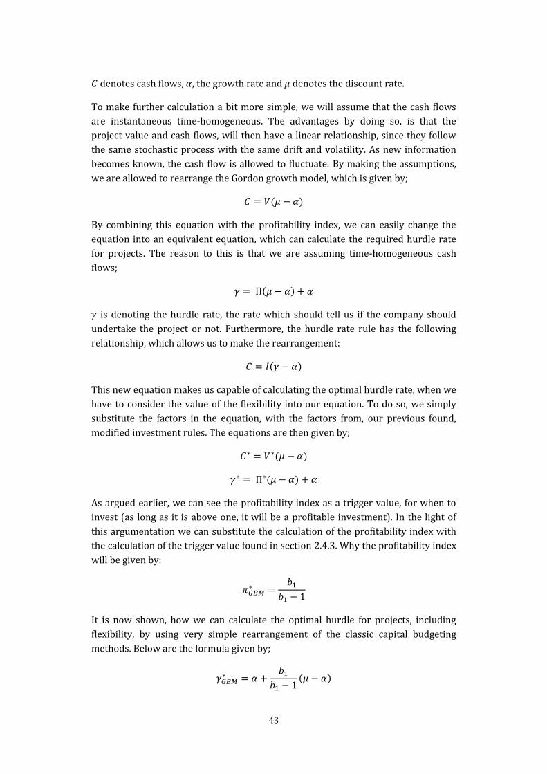
43

denotes cash flows, , the growth rate and denotes the discount rate.

To make further calculation a bit more simple, we will assume that the cash flows

are instantaneous time-homogeneous. The advantages by doing so, is that the

project value and cash flows, will then have a linear relationship, since they follow

the same stochastic process with the same drift and volatility. As new information

becomes known, the cash flow is allowed to fluctuate. By making the assumptions,

we are allowed to rearrange the Gordon growth model, which is given by;

( )

By combining this equation with the profitability index, we can easily change the

equation into an equivalent equation, which can calculate the required hurdle rate

for projects. The reason to this is that we are assuming time-homogeneous cash

flows;

( )

is denoting the hurdle rate, the rate which should tell us if the company should

undertake the project or not. Furthermore, the hurdle rate rule has the following

relationship, which allows us to make the rearrangement:

( )

This new equation makes us capable of calculating the optimal hurdle rate, when we

have to consider the value of the flexibility into our equation. To do so, we simply

substitute the factors in the equation, with the factors from, our previous found,

modified investment rules. The equations are then given by;

( )

( )

As argued earlier, we can see the profitability index as a trigger value, for when to

invest (as long as it is above one, it will be a profitable investment). In the light of

this argumentation we can substitute the calculation of the profitability index with

the calculation of the trigger value found in section 2.4.3. Why the profitability index

will be given by:

It is now shown, how we can calculate the optimal hurdle for projects, including

flexibility, by using very simple rearrangement of the classic capital budgeting

methods. Below are the formula given by;

( )

44

3.2 Discussion of the Characteristics of the

Modified Capital Budgeting Methods

One of the main objectives of this thesis is as mentioned before, to develop heuristic

investment rule or at least show how this can be done for different options. In other

words we create some very simple rules of thumb, where the calculations will be

reasonable close to the ones of the theoretical correct models, which we have

discussed in earlier sections of this paper. Therefore we seek to invest in this section

of the paper, as we did with the theoretical correct model, the relationship between

the parameters in the modified capital budgeting methods model. In later sections

this will provide us with an understanding and a foundation for perhaps dropping

some parameters from the model, maybe both due to their insignificance but maybe

also if they are close to being insignificant and the explanation value they add is

small. If this will come to a reasonable accurate estimate will be discussed in later

sections of this paper.

3.2.1 The Option to Defer

Considering both the modified hurdle rate and the modified profitability index we

start our sensitivity analysis showing that some parameters in both of our modified

models are very sensitive to the value of the parameters, while some are not. We

start out as previously in our base case, in which the respective parameters are

equal to, the risk free rate, = 5 %, risk adjusted expected return, = 25 % and the

growth rate is set equal to zero, = 0 %, and therefore the payout rate, = 25 %, as

discussed in the section of the discussion of the characteristics of the theoretical

model, it is the difference between and . As the modified hurdle rate is obviously

not the same model as the theoretical correct model, the fundamentals of the models

and the way that the parameters interconnect is not the same. Therefore we have to

know both the values of the risk adjusted expected return, and the growth rate,

to validate the modified hurdle rate model. We note in the same time that even

though we do not explicitly need to know in the specific modified model for the

profitability index, both the risk adjusted expected return, and the growth rate,

but infact only the difference between the two parameters, namely the payout ratio,

. Therefore to make our analysis more comparable to the characteristics of the

modified hurdle rate we use the first two mentioned parameters in our analysis also

for the profitability index. In other words in this specific model, the way the risk

adjusted expected return, and the growth rate, interconnect is the same as in the

theoretical correct model, which was derived in section 2.4.3.

In the below Figure 3.1 we show the modified hurdle rate for different values of

uncertainty or volatility. The illustration is in line with our first thought, namely that

45

the uncertainty has a very significant influence on the hurdle rate and therefore our

value is highly sensitive to changes in this parameter. We also show in Figure 3.2 the

modified profitability index as a function of the volatility.

Figure 3.1 – The Modified Hurdle Rate for the

Option to Defer as a function of the Volatility

Figure 3.2 – Profitability Index for the Option

to Defer as a function of the Volatility

From the above Figure 3.1 we see that for the parameter set, = 5 %, = 25 %, = 0

%, the modified hurdle rate is on average is increasing 0.7 percentage point when

volatility is increasing by 2 %. It should be noted that the modified hurdle rate is not

linear. We see from the illustration that the model is slightly exponential, which

means that the changes of the volatility parameter becomes more significant the

higher the base point volatility has.

Considering instead the modified profitability index as a function of the uncertainty

we also see that uncertainty is very significant to the modified investment rule, here

the profitability index, although it is not quite as significant, compared to Fejl!

Henvisningskilde ikke fundet.. We draw the same conclusion from the below

figure as with the modified hurdle rate for an option to defer, which is that the line

are exponential, meaning that the changes in the uncertainty has more effect on the

modified profitability index the higher the volatility is.

Furthermore we can see from the above that the risk adjusted expected return also

has a significant effect on the modified hurdle rate. If we once again base our

parameter set on the before mentioned parameters we see that the relationship

10%

20%

30%

40%

50%

60%

0% 20% 40% 60%

Mo

dif

ied

Hu

rdle

Ra

te

Volatility

r = 5%, μ = 15%, α = 0%

r = 5%, μ = 25%, α = 0%

r = 5%, μ = 35%, α = 0%

0,0

0,5

1,0

1,5

2,0

2,5

0% 20% 40% 60%

Pro

fita

bil

ity

In

de

x

Volatility

r = 5%, μ = 15%, α = 0%

r = 5%, μ = 25%, α = 0%

r = 5%, μ = 35%, α = 0%

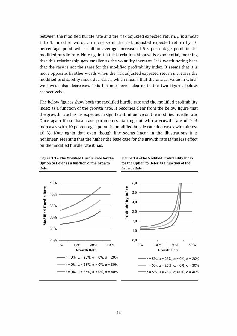
46

between the modified hurdle rate and the risk adjusted expected return, is almost

1 to 1. In other words an increase in the risk adjusted expected return by 10

percentage point will result in average increase of 9.5 percentage point in the

modified hurdle rate. Note again that this relationship also is exponential, meaning

that this relationship gets smaller as the volatility increase. It is worth noting here

that the case is not the same for the modified profitability index. It seems that it is

more opposite. In other words when the risk adjusted expected return increases the

modified profitability index decreases, which means that the critical value in which

we invest also decreases. This becomes even clearer in the two figures below,

respectively.

The below figures show both the modified hurdle rate and the modified profitability

index as a function of the growth rate. It becomes clear from the below figure that

the growth rate has, as expected, a significant influence on the modified hurdle rate.

Once again if our base case parameters starting out with a growth rate of 0 %

increases with 10 percentages point the modified hurdle rate decreases with almost

10 %. Note again that even though line seems linear in the illustrations it is

nonlinear. Meaning that the higher the base case for the growth rate is the less effect

on the modified hurdle rate it has.

Figure 3.3 – The Modified Hurdle Rate for the

Option to Defer as a function of the Growth

Rate

Figure 3.4 –The Modified Profitability Index

for the Option to Defer as a function of the

Growth Rate

20%

25%

30%

35%

40%

45%

0% 10% 20% 30%

Mo

dif

ied

Hu

rdle

Ra

te

Growth Rate

r = 0%, μ = 25%, α = 0%, σ = 20%

r = 0%, μ = 25%, α = 0%, σ = 30%

r = 0%, μ = 25%, α = 0%, σ = 40%

0,0

1,0

2,0

3,0

4,0

5,0

6,0

0% 10% 20% 30%

Pro

fita

bil

ity

In

de

x

Growth Rate

r = 5%, μ = 25%, α = 0%, σ = 20%

r = 5%, μ = 25%, α = 0%, σ = 30%

r = 5%, μ = 25%, α = 0%, σ = 40%

47

The above Figure 3.4 shows the modified profitability index as a function of the

growth rate. This is done for different values of volatility. We note that the effect is

quite different from the effect on the modified hurdle rate. The points in the

illustration can be thought of as different projects with different growth rate and

illustration is in fact the same as Figure 2.4, for the theoretical correct model. We see

that it has exactly the same effect on the critical value as the theoretical correct

model, namely that, if the discount rate or risk adjusted expected return is being

held constant, a decrease in the growth rate, everything else constant the payout

rate will increase which in turn will make the profitability decrease and so will the

critical value. The reason to this, holding everything else constant, should be found

as the expected appreciation of the value increases, it will become more expensive

to wait compared to investing now. The same is happening if the discount rate

increases the critical value will decrease due to a lower profitability index. It

therefore becomes clear that the growth rate has, as expected, a significant influence

on the modified profitability index. It should although be noted that for our specific

set of chosen parameters the growth first becomes very significant at value of more

than 10 %.

In the below figures we have shown both the modified hurdle rate and the modified

profitability index as a function of the risk free rate. It can be seen from the figures

that the risk free rate has a positive correlation with the both modified investment

rules, which makes good sense. This means that as the risk free rate increases, the

critical value will also increase. The reason why is the same as discussed under the

theoretical correct model, which is that a given company due to higher risk free rate

will refrain from investing and therefore fewer options will be exercised due to that

the higher rate will increase the options to invest and therefore also the opportunity

cost by investing now.

48

Figure 3.5 – The Modified Hurdle Rate for the

Option to Defer as a function of the Risk Free

Rate

Figure 3.6 – Profitability Index for the Option

to Defer as a function of the Risk Free

g

3.2.2 The Option to Abandon

We now turn to the discussion of the parameters of the modified hurdle rate and

modified profitability index in relation to the option to abandon. Before we start the

discussion, we note that we would assume the parameters to affect just the opposite

compared to the option to defer, recalling that we are discussing to fundamental

different options, respectively a call and a put option.

In the below figures it can be seen that the volatility parameter has a negative

correlation with the modified hurdle rate. This is obvious since it is now a put

option. In other words when uncertainty about future cash flows is increasing, it is

obviously more difficult to say something about future cash flows, why those are

discounted with a lower modified hurdle rate because it is now an abandon option.

As the hurdle rate decreases it will increase the critical value where a given

company will abandon a given project. It can be seen from the below figure that the

same effect is applicable. Note that this is just the opposite compared to the call

option. Moreover we can see from the below figure that the volatility have, for this

specific set of parameters, surprisingly little affect to the modified hurdle rate.

From Figure 3.9 and Figure 3.10 we see that the effect would have been higher with

a higher value of the risk free rate. This is quite surprising as it points in the same

20%

25%

30%

35%

40%

45%

0% 10% 20% 30%

Mo

dif

ied

Hu

rdle

Ra

te

Risk Free Rate

r = 0%, μ = 25%, α = 0%, σ = 20%

r = 0%, μ = 25%, α = 0%, σ = 30%

r = 0%, μ = 25%, α = 0%, σ = 40%

0,8

1,0

1,2

1,4

1,6

1,8

0% 10% 20% 30%

Pro

fita

bil

ity

In

de

x

Risk Free Rate

r = 0%, μ = 25%, α = 0%, σ = 20%

r = 0%, μ = 25%, α = 0%, σ = 30%

r = 0%, μ = 25%, α = 0%, σ = 40%

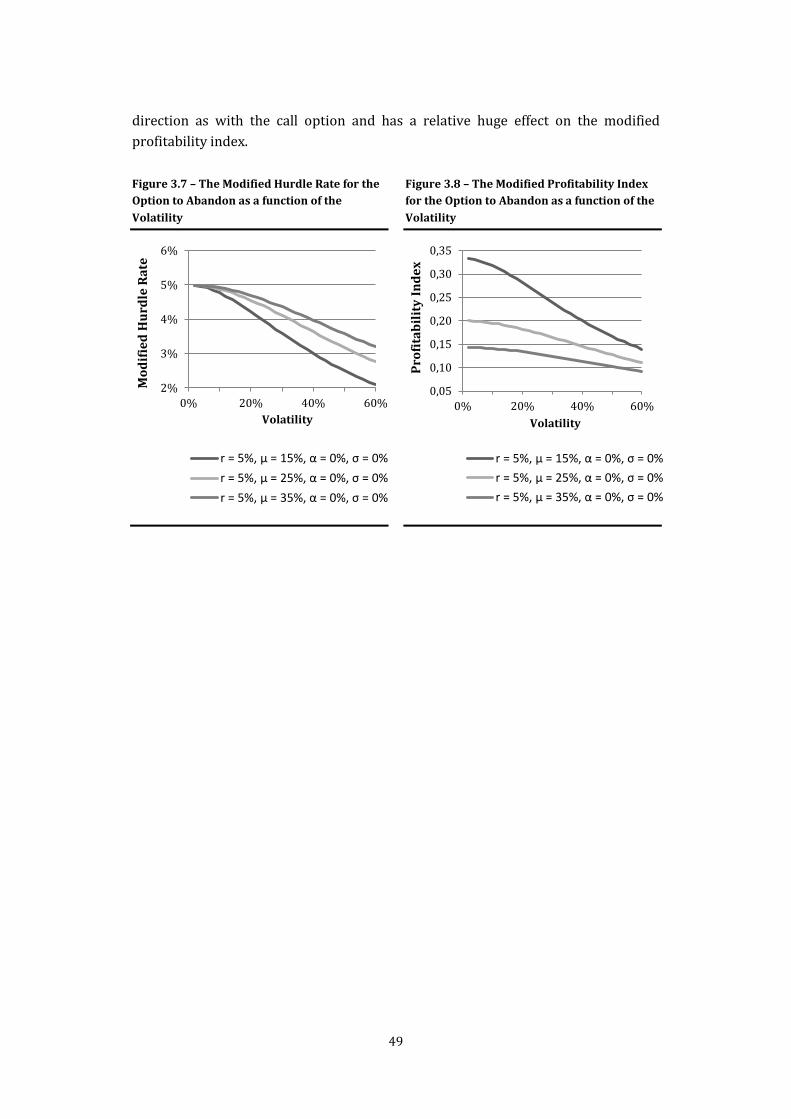
49

direction as with the call option and has a relative huge effect on the modified

profitability index.

Figure 3.7 – The Modified Hurdle Rate for the

Option to Abandon as a function of the

Volatility

Figure 3.8 – The Modified Profitability Index

for the Option to Abandon as a function of the

Volatility

2%

3%

4%

5%

6%

0% 20% 40% 60%

Mo

dif

ied

Hu

rdle

Ra

te

Volatility

r = 5%, μ = 15%, α = 0%, σ = 0%

r = 5%, μ = 25%, α = 0%, σ = 0%

r = 5%, μ = 35%, α = 0%, σ = 0%

0,05

0,10

0,15

0,20

0,25

0,30

0,35

0% 20% 40% 60%P

rofi

tab

ilit

y I

nd

ex

Volatility

r = 5%, μ = 15%, α = 0%, σ = 0%

r = 5%, μ = 25%, α = 0%, σ = 0%

r = 5%, μ = 35%, α = 0%, σ = 0%

50

Figure 3.9 – The Modified Hurdle Rate for the

Option to Abandon as a function of the Risk

Free Rate

Figure 3.10 – The Profitability Index for the

Option to Abandon as a function of the Risk

Free Rate

The reason to this, holding everything else constant, should be found as the expected

appreciation of the value gets higher it will become more expensive to wait

compared to investing now.

At last we consider the effect of a change in the growth rate in relation to both

modified capital budgeting methods. It can be seen from the below Figure 3.12 that

an increase in the growth rate is equivalent with a decrease in the payout rate,

which means that the trigger value will increase and so will the profitability index.

0%

5%

10%

15%

20%

0% 10% 20%

Mo

dif

ied

Hu

rdle

Ra

te

Risk Free Rate

r = 0%, μ = 25%, α = 0%, σ = 20%

r = 0%, μ = 25%, α = 0%, σ = 30%

r = 0%, μ = 25%, α = 0%, σ = 40%

0,0

0,2

0,4

0,6

0,8

0% 10% 20%

Pro

fita

bil

ity

In

de

x

Risk Free Rate

r = 0%, μ = 25%, α = 0%, σ = 20%

r = 0%, μ = 25%, α = 0%, σ = 30%

r = 0%, μ = 25%, α = 0%, σ = 40%

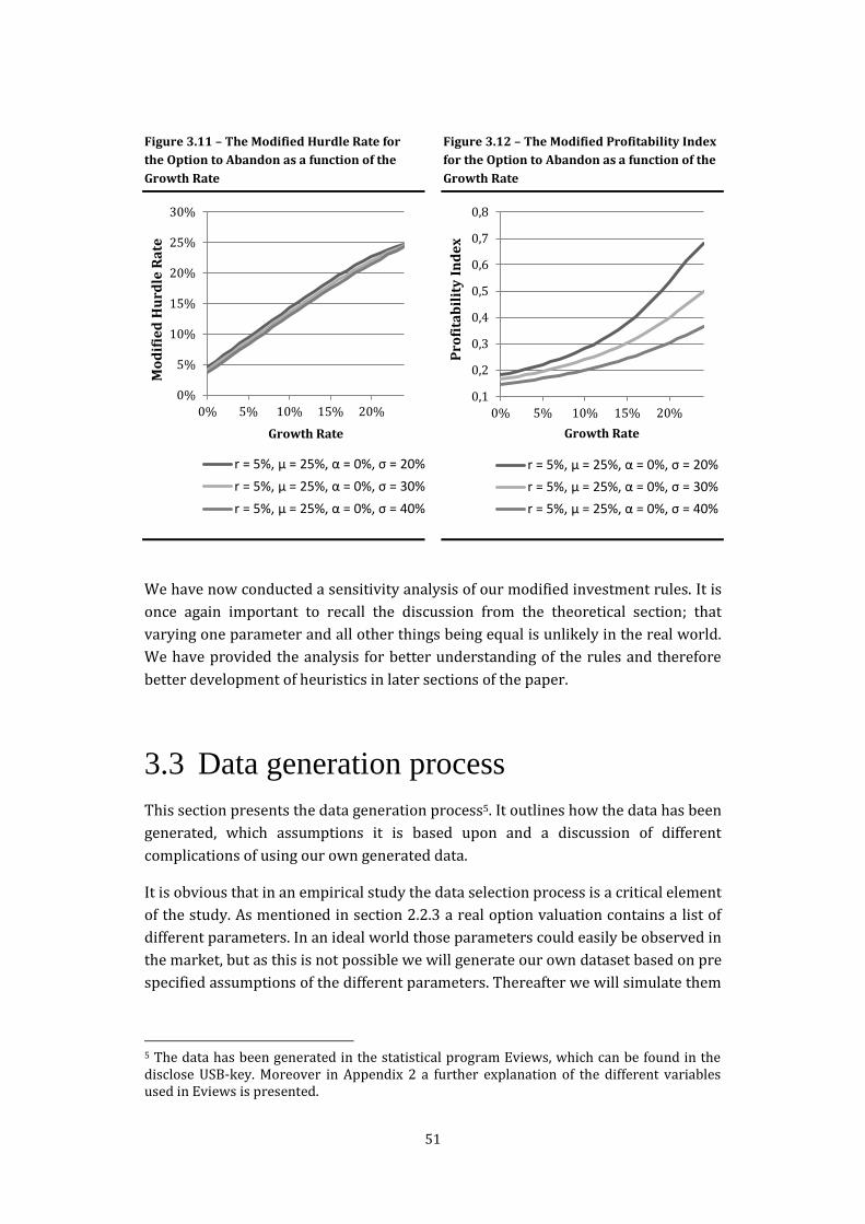
51

Figure 3.11 – The Modified Hurdle Rate for

the Option to Abandon as a function of the

Growth Rate

Figure 3.12 – The Modified Profitability Index

for the Option to Abandon as a function of the

Growth Rate

We have now conducted a sensitivity analysis of our modified investment rules. It is

once again important to recall the discussion from the theoretical section; that

varying one parameter and all other things being equal is unlikely in the real world.

We have provided the analysis for better understanding of the rules and therefore

better development of heuristics in later sections of the paper.

3.3 Data generation process

This section presents the data generation process5. It outlines how the data has been

generated, which assumptions it is based upon and a discussion of different

complications of using our own generated data.

It is obvious that in an empirical study the data selection process is a critical element

of the study. As mentioned in section 2.2.3 a real option valuation contains a list of

different parameters. In an ideal world those parameters could easily be observed in

the market, but as this is not possible we will generate our own dataset based on pre

specified assumptions of the different parameters. Thereafter we will simulate them

5 The data has been generated in the statistical program Eviews, which can be found in the disclose USB-key. Moreover in Appendix 2 a further explanation of the different variables used in Eviews is presented.

0%

5%

10%

15%

20%

25%

30%

0% 5% 10% 15% 20%

Mo

dif

ied

Hu

rdle

Ra

te

Growth Rate

r = 5%, μ = 25%, α = 0%, σ = 20%

r = 5%, μ = 25%, α = 0%, σ = 30%

r = 5%, μ = 25%, α = 0%, σ = 40%

0,1

0,2

0,3

0,4

0,5

0,6

0,7

0,8

0% 5% 10% 15% 20%

Pro

fita

bil

ity

In

de

x

Growth Rate

r = 5%, μ = 25%, α = 0%, σ = 20%

r = 5%, μ = 25%, α = 0%, σ = 30%

r = 5%, μ = 25%, α = 0%, σ = 40%

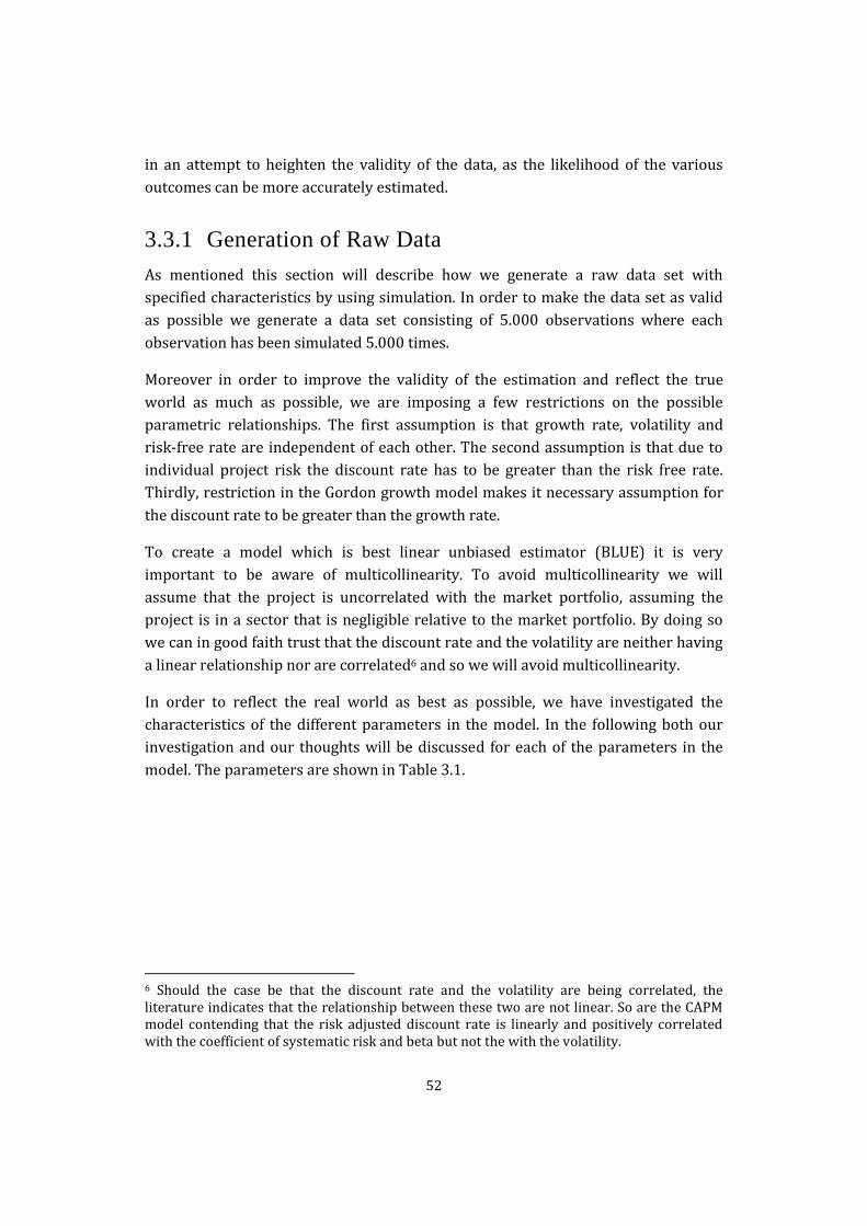
52

in an attempt to heighten the validity of the data, as the likelihood of the various

outcomes can be more accurately estimated.

3.3.1 Generation of Raw Data

As mentioned this section will describe how we generate a raw data set with

specified characteristics by using simulation. In order to make the data set as valid

as possible we generate a data set consisting of 5.000 observations where each

observation has been simulated 5.000 times.

Moreover in order to improve the validity of the estimation and reflect the true

world as much as possible, we are imposing a few restrictions on the possible

parametric relationships. The first assumption is that growth rate, volatility and

risk-free rate are independent of each other. The second assumption is that due to

individual project risk the discount rate has to be greater than the risk free rate.

Thirdly, restriction in the Gordon growth model makes it necessary assumption for

the discount rate to be greater than the growth rate.

To create a model which is best linear unbiased estimator (BLUE) it is very

important to be aware of multicollinearity. To avoid multicollinearity we will

assume that the project is uncorrelated with the market portfolio, assuming the

project is in a sector that is negligible relative to the market portfolio. By doing so

we can in good faith trust that the discount rate and the volatility are neither having

a linear relationship nor are correlated6 and so we will avoid multicollinearity.

In order to reflect the real world as best as possible, we have investigated the

characteristics of the different parameters in the model. In the following both our

investigation and our thoughts will be discussed for each of the parameters in the

model. The parameters are shown in Table 3.1.

6 Should the case be that the discount rate and the volatility are being correlated, the literature indicates that the relationship between these two are not linear. So are the CAPM model contending that the risk adjusted discount rate is linearly and positively correlated with the coefficient of systematic risk and beta but not the with the volatility.

53

Table 3.1 – Parameter Values

Variable Parameter Mean Standard deviation

Project value, investment

cost, scrap value

1

Risk-free Rate 0.05 0.02

Growth Rate 0.045 0.02

Discount Rate 0.10

Volatility 0.30 0.9

Project value, investment costs and scrap value: To keep our later calculation as

simple as possible we have chosen to use a fixed amount of investment costs and

scrap value for our simulated data. When later the critical value and the option value

are calculated it is not the exact value of the costs and the project value that are

critical to our investigations but the difference between them. This means that if we

have project value equal to one, we would have a project with a zero net present

value.

Risk-free rate: The risk-free rate is in its general form defined as a portfolio

without any covariance with the market, which means that it has a CAPM beta of

zero. From a theoretical point of view the risk-free rate is equal to the rate on zero

coupon bonds, which has zero bankruptcy or reinvestment risk and the time horizon

on those bonds matches the returns that should be discounted. This means that

ideally there should be used different risk-free rates to discount the returns for

every single year that should be discounted. In a valuation process this is rarely

done and therefore it is recommended to use a 10-year zero coupon bond. The

reason why the zero coupon bond is being used to reflect the risk-free rate is due to

the ongoing outgoing cash-flow on “normal” bonds, which will have a decreasing

effect on the effective maturity on the bonds compared to the actual maturity. It can

be discussed if a 30-year government bond would be more appropriate to reflect

and match the cash flow but as they are more illiquid the investors will demand

higher premiums, it will not reflect the present value (Koller et al. 2010a). Therefore

we have chosen to use a 10-year government bond.

The risk free rate used in a real option pricing situation should be a rate that reflect

and therefore corresponds to the expiration of the option. As before mentioned we

have assume, in the provided continuous-time model in the section of the theoretical

foundation, that the real option does not expire, which is why we need to find a risk

free rate that reflect this.

54

Koller et al. (2010) recommend the use of the 10-year German government bonds

when valuing European companies due to their liquidity and lower credit risk

compared to bonds from other European countries. We will make use of that.

Moreover as Germany is the biggest economy in Europe it is also seen as the best

estimator of the overall European risk-free rate. It should be mentioned that even

though Koller et al. recommends the use of the German government bond it is also

recommend to always use government bonds in the same currency as the company’s

cash flow or in our case the projects cash flow as it is then possible to model the

inflation consistently between the cash flow and the discount rate. In this case we do

not have a specific currency, why we can easily use the German risk free rate.

To generate a plausible sample of the risk free rate, we have used the monthly

German risk-free rate from January 1989 to July 2014 as a base. Just as the German

risk-free rate our sample have a mean around 5 % and a standard deviation of

around 2 % in a log linear distribution.

Growth rate: According to the European Central Bank the historical GDP of the euro

zone has been 1.8 %7. This seems like the most reliable estimator to use for a future

growth rate. However, it is very low talking real options with a high volatility into

account. Instead it has been decided to use a sample with mean of around 4.5 % and

a standard deviation of 2 % in a log normal distribution.

Discount rate: It is very hard to argue which discount rate is the most appropriate

to use. First of all, project specific capital costs are not equal to capital cost for a

specific company as a whole. This means that even though we might be able to

estimate the capital cost for different companies within different industries we

would still not be able to estimate the capital costs for given projects within

different companies. This is also in line with Dixit (Dixit, Pindyck 1994) as he notes

that “Payout rates on projects vary enormously from one project to another…”, which

is the different between the growth rate and the discount rate. The discount rate is

often set out of a very subjective opinion. In this thesis first of all the discount is set

to be dependent on the growth rate as shown in the above table, in order to follow

the restrictions. Moreover a sample with a high mean is chosen. The reason to this

should be found because of the authors belief about that the underlying assets in

real options often is more volatile compared to the volatility of stocks. All this put

together has resulted in us to use a mean of 25% of the discount rate with a

standard deviation of 10 %, again the sample will be log normal distributed.

7 http://www.ecb.europa.eu/stats/keyind/html/sdds.en.html

55

Volatility: The volatility is difficult to generate. The volatility of the option is of

course very dependent on the underlying asset. The Chicago Board Options

Exchange Market Volatility Index, which is a popular measure of the implied

volatility of S&P 500 index options have between 1990 and June 2014, has an

average value of 19.938. But as Arezki et al. (Arezki, Lederman & Zhao 2014) is

arguing that the volatility for commodities prices have a volatility with a mean of

38.2 %, while the volatility in pharmaceutical industry is assumed to be on a much

lower level, because of patents and individual products, which not have the same

high level of competition we believe that it is reasonable to assume that to have a

mean volatility around 30 % and a standard deviations of 9 % in a log normal

distribution. The log normal distribution is again chosen, as the volatility is a

product of many independent random variables.

3.3.2 Discussion of the Data Set

It would obviously have been much better in an empirical study to collect and make

use of real world data instead of generated data. However, exact data on real options

are very hard to find due to many factors including sensitive company specific

secrets, and for other reasons not accessibly including for instance also a lack of

calculation done by various companies. Instead some papers have tried to account

for the value of real options in other ways. The paper from (Berger, Ofek & Swary

1996), which compares the traditional DCF values with real options values

investigates whether the abandonment options values are reflected in the stock

prices. The whole idea in the paper is that a given firm is at least worth its

discounted cash flow plus a minimum the option to abandon the firm. In relation to

our data discussion, the interesting thing in this study, is how the authors estimated

the option values using the companies’ balance sheet. They created a sample of firms

that sold or liquidated operations. This was done by estimating how many cents per

dollar of book value of each three major asset classifications produces when sold.

With that being mentioned we argue though that to make a sample in a reasonable

amount of observations would take a considerably amount of time. And therefore

we have instead discussed the characteristics of the different parameters. By doing

it is our belief that the parameters assumed for the simulation is quite realistic and

somewhat a good reflection of the real world. Moreover as we are considering a

range of values around the means, it is also not seen as critical to choose the “exact”

best means.

8 http://www.cboe.com/micro/vix/historical.aspx

56

3.4 Statistical Method

By using the statistical method of ordinary least squares (OLS) to estimate the

parameters of the multiple regression models, we will analyze the predicting powers

of independent variables from the real option models on the dependent variable. In

our case it is both the modified hurdle rate and the modified profitability index. In

other words we look into how the different parameters in our contingent claims

analysis affect our modified capital budgeting methods. This is done to estimate the

best possible heuristic rule, which can easily be implemented or serve as a rule of

thumb in a more practical-oriented world. We will develop a very simple model,

which has the purpose of giving the best possible clue of how a real option will affect

a project and which parameters shall be used. The contingent claims analysis model

formulas that have been introduced in this thesis can be a hard to calculate, both

because of their complexity and the input numbers, such as volatility can be hard to

find and/or calculate.

We will instead try to find a linear relationship between the data and the modified

hurdle rate and profitability index. Afterwards we will build a model, from the most

significant data from the regression. This will be done from an OLS regression,

where we will try to build a model, which not have the same accuracy level but can

easily be understood and implemented. This happens from the conviction that it is

better to be nearly right than completely wrong!

The general multiple linear regression model can for the whole population be

written as

Where

is the intercept,

is the parameter associated with

As mentioned in this analysis the statistical methods OLS will be used to estimate

the parameters of the multiple regression model. In order to make a sound valid

analysis of the output from the OLS regression, there are a few restrictions or

assumptions that must be met. In other words the ideal data conditions consist of

five assumptions. These assumptions are called the Gauss-Markov assumptions.

Whether or not the OLS estimator b provides a good approximation to the unknown

57

parameter vector β depends on the assumptions that are made about the

distribution of the error term and its relation to the explanatory variables.

Throughout the thesis we test for these assumptions and if nothing else is

mentioned we assume that the assumptions are satisfied.

In general in relation to the outputs that are being generated from the regressed

models it is often seen that the size on the individual explanatory variables in the

models are commented on. As the marginal effects of those individual variables are

of high interest, we will in the below, when estimating the regression models,

comment on the marginal effects. This is done in order to be able to develop

heuristics later on in the thesis.

It is of course also interesting to see if the explanatory variables actually explain the

dependent variables. However as the independent variables or parameters is

derived from a theoretical and mathematical correct formula according to McDonald

(1986) we are quite sure that our parameters with almost 100 % certainty will

explain the dependent variables.

58

4 Empirical Results

This section of the paper presents the results of our empirical analysis of the

performance of the modified investment rules. The data generated in the preceding

section will be analyzed and tested in different regression models in order to

develop the best heuristic rule for practitioners. In section 4.1 we provide the

results from the option to defer an investment. Section 4.2 and 0 provides

respectively the results from the option to expand a project and the option to

abandon a project.

4.1 The Option to Defer

In this section we will provide an analysis of our empirical results of the option to

defer of both the modified hurdle rate and the modified profitability index.

4.1.1 The Modified Hurdle Rate

To see if our independent variables actually have an effect on our modified hurdle

rate, we will start by considering the first regression model. This includes all the

parameters from the original and theoretical correct model. This is our Model 1 and

it is given by the following regression;

( ) ( ) ( )

The “clean” model without any variables being logged, unfortunately were not

linear, why it cannot be used. This is the reason why the dependent and some of the

explanatory variables has been logged. This little maneuver makes the model a bit

more complex, but ensures the model to pass a Ramsey RESET test, as we can reject

the model to be linear.

59

The results from running the above model and the coming models can be found in the

below Table 4.1. From the result of Model 1 it becomes clear, that the model has a

very close to 100 %. This is of course as mentioned before due to the fact that all of the

variables which have an effect upon the found hurdle rate are included as

explanatory variables. It is important to note that all the variables are strongly

significant with a significant level at 5% and the very high F-statistic indicates a high

goodness of fit.

From the Breusch-Pagan-Godfrey test, which tests for heteroscedasticity we can see

that the model suffers from heteroscedasticity, meaning that the variances of the

unobservable error term are non-constant. Therefore it may vary over the

observations. This is as explained a violation of one of the Gauss-Markov

assumptions, which we assumed to be fulfilled so that the OLS estimator is BLUE. As

heteroscedasticity now appears it means that our OLS is no longer BLUE and to

correct this we have chosen to use the White heteroscedasticity-consistent standard

errors.

60

Table 4.1 – Regression Models for the Modified Hurdle Rate for the Option to Defer

Model 1 Model 2 Model 3

Variable Coefficient t-statistic Coefficient t-statistic Coefficient t-statistic

C 0.291501

(0.004591)

63.49736 0.012750

(0.000436)

29.23456 0.072241

(0.002195)

32.90740

( ) 0.794254

(0.002841)

279.6051

0.973540

(0.001070)

910.1994 0.974879

(0.006550)

148.8355

( ) 0.322289

(0.004028)

80.01457

0.562863

(0.002742)

205.2728

0.719878

(0.030786)

23.38312

0.128304

(0.014788)

8.676366

0.974673 0.995334 0.831228

F-statistic 48056.71 532966.4 24615.83

Note: Standard errors in the parentheses and are white standard errors due to heteroscedasticity problem

The normal reasoning behind real options is that the value of the option is created

through the uncertainty of future parameters. Especially the volatility about future

cash flows has high impact on the option value. Moreover the modified hurdle rate

will of course also be strongly affected by the already used discount rate. As our first

model is a simple level-level model we can easily see from the beta values, that these

two mentioned variables are the parameters with the greatest effect on our

modified hurdle rate. They have the highest beta values. We therefore estimate a

model, only by using the discount rate and volatility as explanatory variables. This is

our Model 2 and it is given by;

From the results of our regression on Model 2 it is seen that has been improved

compared to the previous model where all the independent variables was included.

Taking into consideration that this model has a higher explanatory power than

Model 1, it would be preferred to find the hurdle rate by only using the volatility and

the discount rate, rather than using all the variables. Furthermore, this result

indicates that even though both the risk free rate and the growth rate are highly

significant, according to the t-statistic, they do not influence the hurdle rate very

much. This is further analyzed in the forthcoming sensitivity analysis.

61

Once again the model suffers from heteroscedasticity, which again have been

corrected by the use of White heteroscedasticity-consistent standard errors.

By using only a model consisting of the volatility and the discount rate, we have

managed to come up with a much simpler model, compared to the model including

all the variables. In the same time still a modified hurdle rate, which gives a very

good clue of at what level of hurdle rate should be found. However our model still

consists of a very abstract or subjective parameter, which is the variable volatility.

The volatility can be very hard to determine, and can fluctuate a lot depending on

the underlying asset. A heuristic rule would be easier to implement, understand and

use if it did not involve the volatility. Therefore in the last model, we have tried to

regress a model without the volatility variable and therefore it consists of only the

discount rate as the explanatory variable to our modified hurdle rate. That is our

Model 3 and is given by;

From the results from Model 3, which are given in Table 4.1, we can see that the

has dropped to 83 %. Even though that this value is significant lower compared to

the from the first two models, it is still has a very high explanatory power. This is

in fact a very good indicator of, that even though real option is involved in a project,

the most important factor for valuing the project is still the traditional discount rate.

Furthermore, this indicates, that a project that is “deep in the money” or “deep out of

the money” cannot suddenly be an over or an under investment, only because of

introducing real options. The impact real options have on investments is often

significant, but rarely paramount.

As was the case with the two previous models, this model does also suffer from

heteroscedasticity and the White heteroscedasticity-consistent standard errors have

been used.

4.1.2 Profitability Index

As mentioned in an earlier section, the profitability index is also a very used capital

budgeting method, why we will use the profitability index method to investigate the

optimal trigger point. The first model we will consider given by:

It has not been possible to find a linear model by regressing the variables upon ,

why we instead have used the squared form. Furthermore, it has unfortunately not

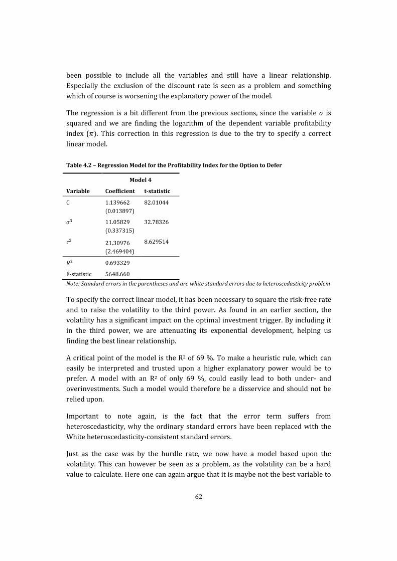
62

been possible to include all the variables and still have a linear relationship.

Especially the exclusion of the discount rate is seen as a problem and something

which of course is worsening the explanatory power of the model.

The regression is a bit different from the previous sections, since the variable is

squared and we are finding the logarithm of the dependent variable profitability

index ( ). This correction in this regression is due to the try to specify a correct

linear model.

Table 4.2 – Regression Model for the Profitability Index for the Option to Defer

Model 4

Variable Coefficient t-statistic

C 1.139662

(0.013897)

82.01044

11.05829

(0.337315)

32.78326

21.30976

(2.469404)

8.629514

0.693329

F-statistic 5648.660

Note: Standard errors in the parentheses and are white standard errors due to heteroscedasticity problem

To specify the correct linear model, it has been necessary to square the risk-free rate

and to raise the volatility to the third power. As found in an earlier section, the

volatility has a significant impact on the optimal investment trigger. By including it

in the third power, we are attenuating its exponential development, helping us

finding the best linear relationship.

A critical point of the model is the R2 of 69 %. To make a heuristic rule, which can

easily be interpreted and trusted upon a higher explanatory power would be to

prefer. A model with an R2 of only 69 %, could easily lead to both under- and

overinvestments. Such a model would therefore be a disservice and should not be

relied upon.

Important to note again, is the fact that the error term suffers from

heteroscedasticity, why the ordinary standard errors have been replaced with the

White heteroscedasticity-consistent standard errors.

Just as the case was by the hurdle rate, we now have a model based upon the

volatility. This can however be seen as a problem, as the volatility can be a hard

value to calculate. Here one can again argue that it is maybe not the best variable to

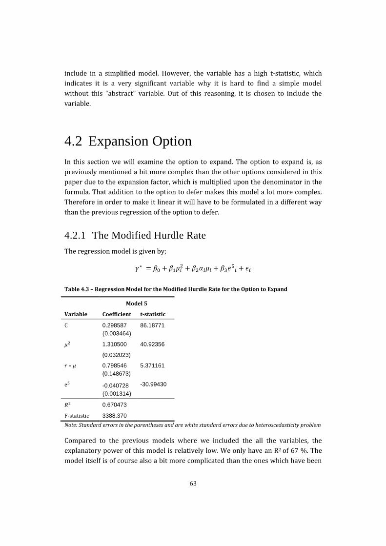
63

include in a simplified model. However, the variable has a high t-statistic, which

indicates it is a very significant variable why it is hard to find a simple model

without this “abstract” variable. Out of this reasoning, it is chosen to include the

variable.

4.2 Expansion Option

In this section we will examine the option to expand. The option to expand is, as

previously mentioned a bit more complex than the other options considered in this

paper due to the expansion factor, which is multiplied upon the denominator in the

formula. That addition to the option to defer makes this model a lot more complex.

Therefore in order to make it linear it will have to be formulated in a different way

than the previous regression of the option to defer.

4.2.1 The Modified Hurdle Rate

The regression model is given by;

Table 4.3 – Regression Model for the Modified Hurdle Rate for the Option to Expand

Model 5

Variable Coefficient t-statistic

C 0.298587

(0.003464)

86.18771

1.310500

(0.032023)

40.92356

0.798546

(0.148673)

5.371161

-0.040728

(0.001314)

-30.99430

0.670473

F-statistic 3388.370

Note: Standard errors in the parentheses and are white standard errors due to heteroscedasticity problem

Compared to the previous models where we included the all the variables, the

explanatory power of this model is relatively low. We only have an R2 of 67 %. The

model itself is of course also a bit more complicated than the ones which have been

64

regressed previously. For the purpose of this thesis, this is also seen as a weakness,

as we are looking for a simple way to calculate a hurdle rate, which will include the

real option.

Just as the case has been previously, the White heteroscedasticity-consistent

standard errors have been used.

Through several tries it has not been possible to find any simpler model. This is an

effect of the model not to have a linear relationship.

4.2.2 The Modified Profitability index

When estimating the best model for explaining the optimal trigger profitability

index by an option to expand, it is unfortunately very hard to estimate a model

which is linear. To follow the Gauss-Markov assumptions and make a line which is

linear, we have been forced to make some adjustment instead of just make a simple

regression: It is very clear that the volatility factor has an enormous impact of the

profitability index, why we have raised the volatility factor to the power of third.

Likewise we have squared the risk free rate, as we know from previous analysis that

this factor has a huge impact as well. Lastly, in order to help the model being linear

we have taken the log of the discount rate, . To have the highest possible

explanatory power, we have in the first regression included all the variables. The

model is therefor given by:

( )

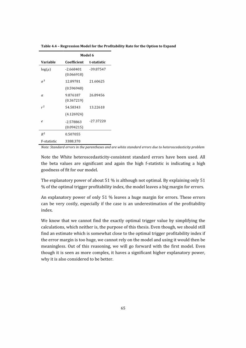
65

Table 4.4 – Regression Model for the Profitability Rate for the Option to Expand

Model 6

Variable Coefficient t-statistic

( ) -2.668401

(0.066918)

-39.87547

12.89781

(0.596948)

21.60625

9.876187

(0.367219)

26.89456

54.58343

(4.126924)

13.22618

-2.578863

(0.094215)

-27.37220

0.507055

F-statistic 3388.370

Note: Standard errors in the parentheses and are white standard errors due to heteroscedasticity problem

Note the White heteroscedasticity-consistent standard errors have been used. All

the beta values are significant and again the high f-statistic is indicating a high

goodness of fit for our model.

The explanatory power of about 51 % is although not optimal. By explaining only 51

% of the optimal trigger profitability index, the model leaves a big margin for errors.

An explanatory power of only 51 % leaves a huge margin for errors. These errors

can be very costly, especially if the case is an underestimation of the profitability

index.

We know that we cannot find the exactly optimal trigger value by simplifying the

calculations, which neither is, the purpose of this thesis. Even though, we should still

find an estimate which is somewhat close to the optimal trigger profitability index if

the error margin is too huge, we cannot rely on the model and using it would then be

meaningless. Out of this reasoning, we will go forward with the first model. Even

though it is seen as more complex, it haves a significant higher explanatory power,

why it is also considered to be better.

66

4.3 Option to abandon

4.3.1 The Modified Hurdle Rate

In the following section the modified hurdle rate with the option to abandon a

project will be analyzed. This will be done in the same way as the previous section,

whereas the first regression model will consist of all the parameters, which are a

part of the theoretically and mathematically correct solution to the option to

abandon. Just like in the first part our Model 7 is given by

Table 4.5 – Regression models for Modified Hurdle Rate for the Option to Abandon

Model 7 Model 8 Model 9

Variable Coefficient t-statistic Coefficient t-statistic Coefficient t-statistic

C 0.008573

(0.000318)

26.99804 0.002199

(0.000366)

6.016247

0.035510

(0.000769)

46.15066 0.320221

(0.005751)

55.67694

-0.049197

(0.000711)

-69.19884

0.749433

(0.005155)

145.3763 0.754391

(0.007454)

101.2122

0.965580

(0.001196)

807.4114 1.002897

(0.001979)

506.6636

0.995692 0.982263 0.313603

F-statistic 288628.8 138368.8

Note: Standard errors in the parentheses and are white standard errors due to heteroscedasticity problem

From the results of Model 7 we see once again that has a value very close to

100%, which were just as expected, since the parameters used in the formula were

the same used to generate the hurdle rates through the formula. It is important to

note that it is that just like in the previous cases, the model was found to suffer from

heteroscedasticity and the standard errors were therefore replaced with the White

heteroscedasticity-consistent standard errors. None of the beta values were found to

be insignificant at a significance level at 95 %, which is implying that all of the

parameters have some kind of effect upon our final hurdle rate. Again, just as the

67

cases were by the option to defer, the high f-statistic is indicating that our models

have a high goodness of fit.

The option to abandon is very different to the option to defer, why the fundamental

logic behind is also very different, in some way the opposite. This is of course due to

fact that it is a put and a call option. This fact is also supported by the beta values in

the regression, which is very different from the beta values in the first regression.

Where and were the two most explaining coefficients by the option to defer, it is now

r and g which is the most explanatory variables.

However, the result is found to be a bit surprising. The value of real option is often

argued to be the volatility, but in this regression the volatility has a very low beta

value, which indicates that the volatility has a very low effect on the level of the

hurdle rate. Furthermore, the hurdle rate is somewhat a corrected discount rate, as

we try to incorporate the flexibility into classic capital budgeting method.

Surprisingly the already existing discount rate does not affect the hurdle rate a lot.

In fact, with a beta value of only 0.035 the discount rate has the lowest beta value

besides the constant.

As the and the did not have the biggest impact upon the hurdle rate, we will

make a new regression leaving out these two parameters, just as we did in the

option to defer, where we left out the r and g. The purpose of doing so, is of course to

find and develop the most appropriate and simple heuristic rule.

Furthermore, by leaving out especially the volatility ( ), we are getting rid of a very

complex factor. The volatility can as mentioned before in this thesis be very hard to

estimate and determine and therefor by leaving it out we can maybe develop a very

simple heuristic. We name this regression Model 5 and it is given by

Just like in the previous regression, the standard errors have suffered from

heteroscedasticity, which is why they have been replaced with the White

heteroscedasticity-consistent standard errors. All of the beta values are still very

significant at a significance level of 95 %.

Even though we have left out the volatility and the discount rate, we still have a

very close to the 100 %, which for us is a very surprising finding, especially since we

consider the volatility as the most important parameter in the real option

terminology before these findings. When analyzing the beta values, we see that

especially the growth rate has a very huge impact on the hurdle rate. Every time the

growth rate rises by one, the hurdle rate should rise with a bit more, indicating that

68

when the growth rate rises, the option value of an abandonment option will fall. This

is due to the fact that the value of a put option is found in the insurance of the

downside risk, which will be lower with a high growth rate.

Just as we did by the option to defer, we will examine how huge an impact the real

option has on the new hurdle rate. This will be done, just as we did previous, by

regression only the discount rate upon the hurdle rate. The regression will be given

by:

Due to the fact that the constant was very insignificant, this has not been included in

the regression. Important to note also, is that just like in the other regressions the

White heteroscedasticity-consistent standard errors have been used, to fix the issue

with heteroscedasticity.

From the beta values, we can see the discount rate itself has an explanatory power

of 31 %. Compared to the option to defer where the discount rate had an

explanatory power of 85 %, the explanatory power of the discount rate in the option

to abandon is relatively low.

However with an explanatory power of 31% there is still some value in knowing the

discount rate found by the classical capital budgeting methods. But the regression

shows the importance to consider the flexibility, the real options is giving, before

making any investment decisions. If the real options are not considered in the

investment considerations, one is risking making over or under investments.

Instead a regression shows that the growth rate has a relatively high impact upon

the modified hurdle rate of option to abandon. With an explanatory power of 85 %,

the growth rate is quite significant, and should be accounted when taking a decision

of holding on to the an investment or liquidating it.

69

Table 4.6 – Regression models for Modified Hurdle Rate for the Option to Abandon

Model 10

Variable Coefficient t-statistic

C 0.043415

(0.000426)

101.9478

0.998063

(0.005957)

167.5341

0.848846

F-statistic 28067.67

Note: Standard errors in the parentheses and are white standard errors due to heteroscedasticity problem

4.3.2 The Modified Profitability Index

When we shall find a simpler way to calculate the profitability index for the

abandonment option, we know from the hurdle rate regression, that the most

significant factors were the growth rate and the risk-free rate. By focusing on them,

we can then find the model with the highest explanatory power. First we focus on

including all the variables, in hopes of getting the best possible explanatory power.

The regression is given by;

√

70

Table 4.7 – Regression models for Profitability Index for the Option to Abandon

Model 11 Model 12

Variable Coefficient t-statistic Coefficient t-statistic

C 0.343193

(0.001637)

209.6118 0.329488

(0.002741)

120.2179

-1.432560

(0.013728)

-104.3525 -1.302353

(0.028327)

-45.97569

2.947552

(0.083762)

35.18963 1.545328

(0.043622)

35.42561

3.364351

(0.018437)

182.4823 3.352587

(0.029320)

114.3438

-0.459145

(0.025093)

-18.29752

0.900910 0.894268

F-statistic 11353.37 14085.15

Note: Standard errors in the parentheses

Again the White heteroscedasticity-consistent standard errors have been used to

make up for the heteroscedasticity. The R2 of 90% is seen as high explanatory

variable, and fulfill our objective to give a slightly right estimation of the optimal

trigger profitability index. All of the beta variables are significant, but in opposition

to the hurdle rate model, the growth rate does not stand out as one of the most

significant factors anymore. The t-statistic shows us that the significance of the beta

values is pretty much in level.

The model will now be reduced. Again, this is done in hopes of getting the simplest

model, without the explanatory power has to suffer too much. If we reduce the level

model, and eliminate some of the variables, we can estimate a model which instead

is given by:

√

We now have a linear model with an explanatory power of 89 % - very close to the

90 % found in the previous model. As the other models it is suffering from

heteroscedasticity why we have chosen to use the White heteroscedasticity-

consistent standard errors. All of the beta variables are significant and the f-statistic

is very high, indicating we have a high goodness-of-fit.

The only critical point of the model is fact, that it has not managed us to leave out

other variables than the growth rate, why it has not become much simpler. On the

71

positive side, the elimination of the growth rate has only cost 0.6 % of the

explanatory power. In this thesis, the purpose is to make the make simple model,

which easily can be interpreted and calculated. The models found for the optimal

trigger profitability index for abandon option, is unfortunately a bit more

complicated than hoped for. However, the model is still simpler to use than the

original, and with a high explanatory power, it gives a good estimation. Out of this

conclusion we will continue working with the second model.

72

5 Heuristic Investment

Rules

In this section of the paper, we present the development of heuristic investment

rules. The foundation for developing heuristic investment rules have been obtained

in the preceding sections of this paper. Thus we first, in section 5.1 develop some

heuristic investment rules. And as the objective of this section of the paper is to

develop some heuristic investment rules that easily can be used of practitioners, we

will in section 5.2 discuss if the developed heuristic rules give a reasonable accurate

estimate.

5.1 Development of Heuristic

Investment Rules

We have in the preceding sections of the paper established a thorough

understanding of the different parameters in the provided modified capital

budgeting methods, through first a sensitivity analysis and thereafter a regression

analysis. This examined both the impact that each variable have on the value of the

option, the cost of changing the variables. This provides a foundation to develop the

best possible composition of the models in order to make the best heuristic

investment rules. We will in the following, based on section 4, pick the best models

and rewrite them in an attempt to find the most simple form of the model and

thereby find the best possible heuristic investment rule in a very simple form, which

will seem easy to use for a practitioner.

73

5.1.1 The Option to Defer

Investigation of the characteristics of the modified capital budgeting of the option to

defer revealed, among other things, that the uncertainty had a very high impact on

the value of both the modified hurdle rate and the modified profitability index. The

effect of a change in the volatility on the modified hurdle rate was around the same

for different values of the risk adjusted expected return, whereas it was quite

different for the modified profitability. Here the effect of a change in the volatility

was quite dependent on the level of the risk adjusted expected return. Although we

still showed that the parameter had an impact.

Furthermore, in the regression analysis of the modified models, we found a great

explanatory power by using only the volatility and the risk adjusted expected return

as explanatory variables, which are in line with our sensitivity analysis of the

modified capital budgeting methods. The authors of this paper would like to discard

the volatility parameter as this parameter can be very hard to estimate and

therefore very subjective, especially if the underlying asset is one without any

historical data such as it most often will be the case for a project.

5.1.1.1 The Modified Hurdle Rate

For the modified hurdle rate we found the beta values to be the following,

(volatility) and (discount rate) with a constant of

0.012750. In an attempt to simplify the model and knowing from section 2.4.5 that a

relative little change will not affect the critical value so much that the result will not

be reasonable accurate, the numbers in the following heuristic models are rounded

and therefore our first heuristic investment rule will be given by;

The reason to the above number rounding is, as mentioned before, due to the fact

that the investigated option values are not normal distributed and therefore the loss

is asymmetric, which is why it seems better to wait too long rather than invest too

early.

5.1.1.2 The Modified Profitability Index

In the same way as above, where we provided a simple heuristic rule for the

modified hurdle rate, we also provide a simple rule for the modified profitability

index. The most simple regression model we have estimated suffers although

unfortunately of a low explanatory power, at least compared to the model above for

the hurdle rate. A of only 69 % leaves a very big error margin. As discussed above

74

especially an underestimation could lead to a very wrong estimation of the

profitability index.

Even though the model is not considered to be very good it is still used as a base for

development of a heuristic investment rule. But in an attempt to improve the model

above, we will need to manipulate the model a bit, whereas we will change the beta

values, some more than others.

From the regression analysis we found the beta values as the following,

(risk-free rate) and (volatility) with a constant

of . By changing an manipulate the results from the analysis, mainly by

rounding them upwards, we have obtained the following heuristic rule for the

modified profitability index for the option to defer;

5.1.2 The Option to Expand

As explained in earlier section of the thesis, the characteristics of the option to

expand are the same as the characteristics for the option to defer except the factor ,

which is a fraction of the value of a project. Therefore changing the different

parameters individual all other things being equal will lead to the same results as for

the option to defer. But as we saw in the regression analysis of the option to expand

the factor e made the model act in a very nonlinear way, which also in the following

is reflected of some rather complex heuristic rules for this specific option.

5.1.2.1 The Modified Hurdle Rate

The beta values for the regression were found to be (discount rate) +

(the risk free rate and discount rate) (expansion

factor) with a constant of 0.298587

Unfortunately, the model only has an R2 of 67% and as described in section this big

error margin can be costly. Especially if the error is an underinvestment of the

hurdle rate, it is costly. To meet this problem, we have made adjustments, which will

deliberately overestimate the hurdle rate. The reason to this is that the

overestimations will not be penalized just as hard, why it is preferred. Because of

the same reason the beta 3 value has not been rounded to 1.3 as it normally would.

Instead it has been made 1.4. The heuristic rule is given by:

75

5.1.2.2 The Modified Profitability Index

The model found through the regression, to build the heuristic rule around, was not

as good as one could have hoped for. The objective of finding a simple model, was

not met, due to the fact that it was very hard to find a linear relation. Moreover, the

model suffers with the highest explanatory power was chosen in front of the simpler

model. The model is thus somewhat complex and not as simple as hoped. Given the

fact that this model has an explanatory power of 51 % it is although a preferable

model.

The beta values was found to be (growth rate),

(risk-free rate), ( ) (discount rate),

(volatility) and (expansion factor), with an insignificant constant.

Once again we would of course rather overestimate than underestimate. This does

not lead to the same level of mistakes as an underestimation would do. From this

conviction we would primarily round the numbers of the regression to a higher

value. Therefore the heuristic rule is given by:

( )

5.1.3 The Option to Abandon

As previously mentioned the fundamentals of the option to abandon are different

compared to the two above discussed options. Therefore the calculation is also a bit

different from the two options above. In the sensitivity analysis we found that the

volatility did not have any huge impact on the modified capital budgeting methods

and therefore also the critical value. In contrast, also to the call option, the risk free

rate and the growth rate seemed to have great impact on the trigger value. Our

subsequent regression analysis was very much in line with those conclusions as we

also here found that the risk free rate and the growth rate is the parameters with the

greatest effect on the modified models.

Important to note, before turning to the heuristic investment rules of the

abandoning option, is that as the calculation in the model make use of instead of

an underestimation is not what we are afraid of. In contrast to the call option it is

overestimation of the modified methods and thereby and overestimation of critical

value. This will lead to that the assets are being liquidated too early and a possible

upside will go lost.

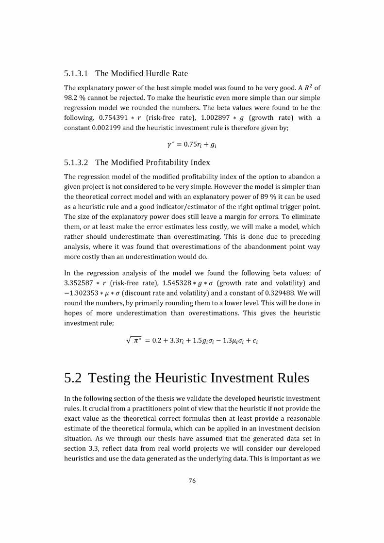
76

5.1.3.1 The Modified Hurdle Rate

The explanatory power of the best simple model was found to be very good. A of

98.2 % cannot be rejected. To make the heuristic even more simple than our simple

regression model we rounded the numbers. The beta values were found to be the

following, (risk-free rate), (growth rate) with a

constant 0.002199 and the heuristic investment rule is therefore given by;

5.1.3.2 The Modified Profitability Index

The regression model of the modified profitability index of the option to abandon a

given project is not considered to be very simple. However the model is simpler than

the theoretical correct model and with an explanatory power of 89 % it can be used

as a heuristic rule and a good indicator/estimator of the right optimal trigger point.

The size of the explanatory power does still leave a margin for errors. To eliminate

them, or at least make the error estimates less costly, we will make a model, which

rather should underestimate than overestimating. This is done due to preceding

analysis, where it was found that overestimations of the abandonment point way

more costly than an underestimation would do.

In the regression analysis of the model we found the following beta values; of

(risk-free rate), (growth rate and volatility) and

(discount rate and volatility) and a constant of We will

round the numbers, by primarily rounding them to a lower level. This will be done in

hopes of more underestimation than overestimations. This gives the heuristic

investment rule;

√

5.2 Testing the Heuristic Investment Rules

In the following section of the thesis we validate the developed heuristic investment

rules. It crucial from a practitioners point of view that the heuristic if not provide the

exact value as the theoretical correct formulas then at least provide a reasonable

estimate of the theoretical formula, which can be applied in an investment decision

situation. As we through our thesis have assumed that the generated data set in

section 3.3, reflect data from real world projects we will consider our developed

heuristics and use the data generated as the underlying data. This is important as we

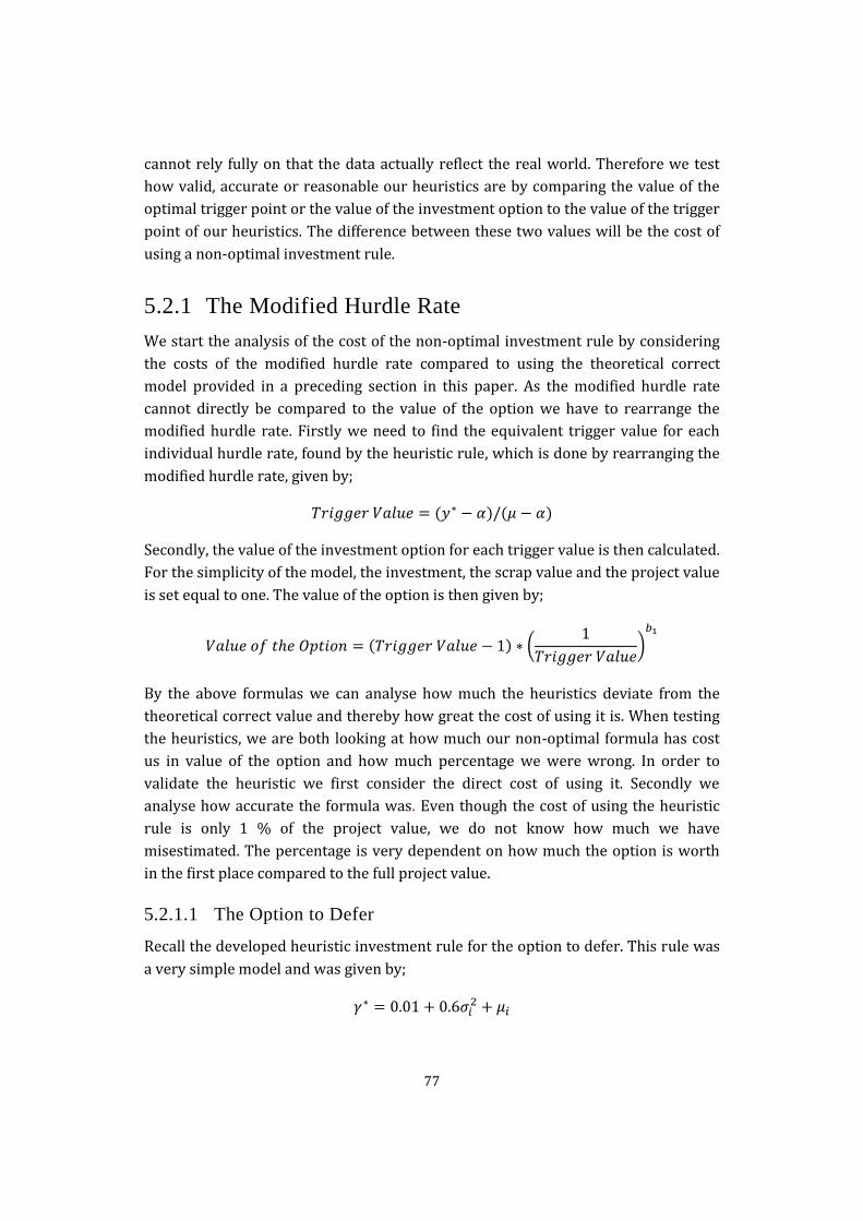
77

cannot rely fully on that the data actually reflect the real world. Therefore we test

how valid, accurate or reasonable our heuristics are by comparing the value of the

optimal trigger point or the value of the investment option to the value of the trigger

point of our heuristics. The difference between these two values will be the cost of

using a non-optimal investment rule.

5.2.1 The Modified Hurdle Rate

We start the analysis of the cost of the non-optimal investment rule by considering

the costs of the modified hurdle rate compared to using the theoretical correct

model provided in a preceding section in this paper. As the modified hurdle rate

cannot directly be compared to the value of the option we have to rearrange the

modified hurdle rate. Firstly we need to find the equivalent trigger value for each

individual hurdle rate, found by the heuristic rule, which is done by rearranging the

modified hurdle rate, given by;

( ) ( )

Secondly, the value of the investment option for each trigger value is then calculated.

For the simplicity of the model, the investment, the scrap value and the project value

is set equal to one. The value of the option is then given by;

( ) (

)

By the above formulas we can analyse how much the heuristics deviate from the

theoretical correct value and thereby how great the cost of using it is. When testing

the heuristics, we are both looking at how much our non-optimal formula has cost

us in value of the option and how much percentage we were wrong. In order to

validate the heuristic we first consider the direct cost of using it. Secondly we

analyse how accurate the formula was. Even though the cost of using the heuristic

rule is only 1 % of the project value, we do not know how much we have

misestimated. The percentage is very dependent on how much the option is worth

in the first place compared to the full project value.

5.2.1.1 The Option to Defer

Recall the developed heuristic investment rule for the option to defer. This rule was

a very simple model and was given by;

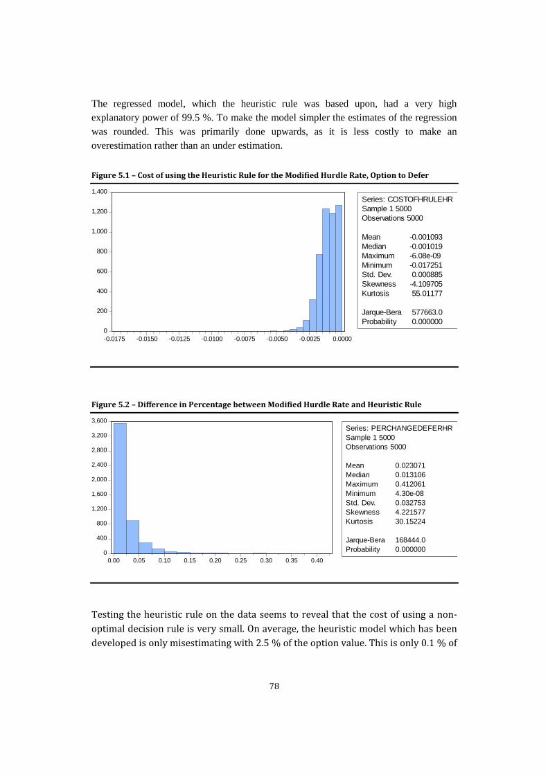
78

The regressed model, which the heuristic rule was based upon, had a very high

explanatory power of 99.5 %. To make the model simpler the estimates of the regression

was rounded. This was primarily done upwards, as it is less costly to make an

overestimation rather than an under estimation.

Figure 5.1 – Cost of using the Heuristic Rule for the Modified Hurdle Rate, Option to Defer

0

200

400

600

800

1,000

1,200

1,400

-0.0175 -0.0150 -0.0125 -0.0100 -0.0075 -0.0050 -0.0025 0.0000

Series: COSTOFHRULEHR

Sample 1 5000

Observations 5000

Mean -0.001093

Median -0.001019

Maximum -6.08e-09

Minimum -0.017251

Std. Dev. 0.000885

Skewness -4.109705

Kurtosis 55.01177

Jarque-Bera 577663.0

Probability 0.000000

Figure 5.2 – Difference in Percentage between Modified Hurdle Rate and Heuristic Rule

0

400

800

1,200

1,600

2,000

2,400

2,800

3,200

3,600

0.00 0.05 0.10 0.15 0.20 0.25 0.30 0.35 0.40

Series: PERCHANGEDEFERHR

Sample 1 5000

Observations 5000

Mean 0.023071

Median 0.013106

Maximum 0.412061

Minimum 4.30e-08

Std. Dev. 0.032753

Skewness 4.221577

Kurtosis 30.15224

Jarque-Bera 168444.0

Probability 0.000000

Testing the heuristic rule on the data seems to reveal that the cost of using a non-

optimal decision rule is very small. On average, the heuristic model which has been

developed is only misestimating with 2.5 % of the option value. This is only 0.1 % of

79

the project value, and with a standard deviation of 0.2. Note though that even though

this might seem as a small error it is still a significant error.

Table 5.1 – Paired t-test for the Modified Hurdle Rate for the Option to Defer

Value Probability

Test of Hypothesis (mean) 0

Sample Mean -0.001093

Sample Std. Dev. 0.000885

t-statistic -87.33718 0.0000

The mean have been tested through a simple paired t-test. A t-statistic of -87.34 has

been found, which is implying that the mean cost is very significant. This result

implies that there is a different between the values of the right trigger point and the

trigger point found through the use of the developed heuristics. Furthermore it

implies that there is a cost associated with the use of the heuristic.

Even though there is a cost associated with the use of this heuristic rule, this cost is

relatively small – only 0.1 % of the project value in average. Therefor this heuristic

can be used as at least as a good indicator of where the optimal trigger point is at.

The heuristic is considered as a decent alternative to the original model.

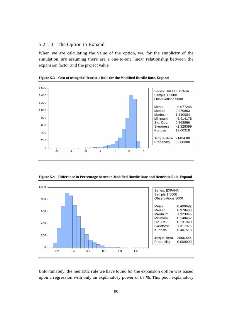
80

5.2.1.3 The Option to Expand

When we are calculating the value of the option, we, for the simplicity of the

simulation, are assuming there are a one-to-one linear relationship between the

expansion factor and the project value

Figure 5.3 – Cost of using the Heuristic Rule for the Modified Hurdle Rate, Expand

0

200

400

600

800

1,000

1,200

1,400

1,600

-5 -4 -3 -2 -1 0 1

Series: HRULEEXPAHR

Sample 1 5000

Observations 5000

Mean -0.077245

Median 0.079853

Maximum 1.110084

Minimum -5.414178

Std. Dev. 0.568956

Skewness -2.328399

Kurtosis 12.00318

Jarque-Bera 21404.80

Probability 0.000000

Figure 5.4 – Difference in Percentage between Modified Hurdle Rate and Heuristic Rule, Expand

0

200

400

600

800

1,000

0.2 0.4 0.6 0.8 1.0 1.2

Series: EXPAHRSample 1 5000Observations 5000

Mean 0.400692Median 0.378463Maximum 1.323046Minimum 0.140462Std. Dev. 0.131940Skewness 1.317975Kurtosis 6.407518

Jarque-Bera 3866.544Probability 0.000000

Unfortunately, the heuristic rule we have found for the expansion option was based

upon a regression with only an explanatory power of 67 %. This poor explanatory

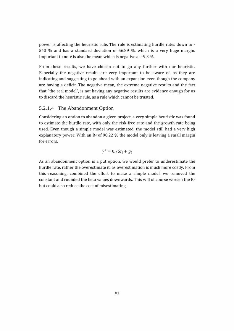
81

power is affecting the heuristic rule. The rule is estimating hurdle rates down to -

543 % and has a standard deviation of 56.89 %, which is a very huge margin.

Important to note is also the mean which is negative at –9.3 %.

From these results, we have chosen not to go any further with our heuristic.

Especially the negative results are very important to be aware of, as they are

indicating and suggesting to go ahead with an expansion even though the company

are having a deficit. The negative mean, the extreme negative results and the fact

that “the real model”, is not having any negative results are evidence enough for us

to discard the heuristic rule, as a rule which cannot be trusted.

5.2.1.4 The Abandonment Option

Considering an option to abandon a given project, a very simple heuristic was found

to estimate the hurdle rate, with only the risk-free rate and the growth rate being

used. Even though a simple model was estimated, the model still had a very high

explanatory power. With an R2 of 98.22 % the model only is leaving a small margin

for errors.

As an abandonment option is a put option, we would prefer to underestimate the

hurdle rate, rather the overestimate it, as overestimation is much more costly. From

this reasoning, combined the effort to make a simple model, we removed the

constant and rounded the beta values downwards. This will of course worsen the R2

but could also reduce the cost of misestimating.

82

Figure 5.5 – Cost of using the Heuristic Rule for the Modified Hurdle Rate, Abandon

0

1,000

2,000

3,000

4,000

5,000

-0.12 -0.10 -0.08 -0.06 -0.04 -0.02 0.00

Series: COSTOFRULEHR2

Sample 1 5000

Observations 5000

Mean -0.001711

Median -0.000904

Maximum -1.26e-10

Minimum -0.117131

Std. Dev. 0.004244

Skewness -13.46590

Kurtosis 269.4859

Jarque-Bera 14945844

Probability 0.000000

Figure 5.6 – Difference in Percentage between Modified Hurdle Rate and Heuristic Rule, Expand

0

1,000

2,000

3,000

4,000

5,000

0.00 0.05 0.10 0.15 0.20 0.25 0.30 0.35 0.40 0.45 0.50

Series: PERCHANGEABANDHR

Sample 1 5000

Observations 5000

Mean 0.003480

Median 0.001510

Maximum 0.494766

Minimum 2.27e-10

Std. Dev. 0.012730

Skewness 23.29565

Kurtosis 746.7642

Jarque-Bera 1.16e+08

Probability 0.000000

As we see the above Figure 5.5 the cost of using the heuristic rule and misestimating

is very low. On average the cost is only 0.17 % of the project value, which is seen as a

relative small cost. With a mean of 0.17 % and a standard deviation of 0.42 % it is

also very interesting to see that the median of the misestimating is only 0.09 % of

the project value. Likewise, the misestimating of the option value is only 0.3 % and

has a standard deviation of 1.2 %, why this is not significantly destroying value of

our project and we must consider the heuristic as reasonable accurate for

practitioners.

83

Table 5.2 – Paired t-test for the Modified Hurdle Rate for the Option to Abandon

Value Probability

Test of Hypothesis (mean) 0

Sample Mean -0.001711

Sample Std. Dev. 0.004244

t-statistic -28.51615 0.0000

To test whether or not the use of the heuristics is significantly destroying value of

projects with real options included a simple t-test has again been performed.

Through this t-test a value of -28.5 was found, which indicates that the cost is quite

significant. This implies that even though the cost of using the heuristic is relatively

low, it is a significant cost.

However taking into account that the heuristic is giving a trigger value which is

leading to an option value only 3 % lower than the original one on average, the

heuristic rule have some value. It is a much simpler model and both the risk free rate

and the growth rate should be easy numbers to estimate, in opposition to volatility

which is eliminated. From this philosophy the heuristic rule is seen as a decent

alternative to the original model.

84

5.2.3 Profitability index

5.2.3.1 The Option to Defer

Figure 5.7 – Cost of using the Heuristic Rule for the Profitability Index, Defer

0

400

800

1,200

1,600

2,000

2,400

-0.06 -0.05 -0.04 -0.03 -0.02 -0.01 0.00

Series: COSTOFTHEURISTICPI

Sample 1 5000

Observations 5000

Mean -0.004500

Median -0.002829

Maximum -2.44e-10

Minimum -0.058151

Std. Dev. 0.005102

Skewness -2.321605

Kurtosis 13.02404

Jarque-Bera 25425.17

Probability 0.000000

Figure 5.8 – Difference in Percentage between Profitability Index and Heuristic Rule, Defer

0

400

800

1,200

1,600

2,000

2,400

0.0 0.1 0.2 0.3 0.4 0.5 0.6 0.7 0.8 0.9

Series: PERCHANGEDEFERPI

Sample 1 5000

Observations 5000

Mean 0.090576

Median 0.036574

Maximum 0.948691

Minimum 3.04e-09

Std. Dev. 0.136527

Skewness 2.683314

Kurtosis 11.51707

Jarque-Bera 21112.73

Probability 0.000000

85

The fact that the heuristic rule is based upon a model with a R2 of 69 % will, all other

things being equal, give a much weaker model compared to the model we found to

estimate the modified hurdle rate for the option to defer.

Using the developed heuristic investment rule will lead to a cost of 0.45 % relative

to the original project value with a standard deviation of 0.51 %. Even though it does

not sound of a lot, it can easily be a significant value, when huge amounts are

invested. Compared to the better model found for the hurdle rate, it is four times as

big.

The value of the option itself is only in average 9 % away from the real value if the

heuristic rule is used instead of the “real” model. With a standard deviation of 13.6

%, the 9 % is a relative high average misestimation, compared to earlier examples

where the mean cost where at 0.3 % and 2 %.

Table 5.3 – Paired t-test for the Profitability Index for the Option to Defer

Value Probability

Test of Hypothesis (mean) 0

Sample Mean 0.005102

Sample Std. Dev. 0.000885

t-statistic -62.37339 0.0000

Through the t-test were we are finding a t-value of -62 we can again clearly see that

the cost of using the heuristic model is very significant.

Even though the model is not as precise as the previous found heuristic rules and

the found trigger value is leading to a 9 % lower average value than the original

model, the heuristic rule is seen as a good indicator of the where the level of the

trigger value should be found. However we argue that a practitioner should favor

the modified hurdle rate over the above modified profitability index as the cost of

using the first mentioned modified investment rule is less than the above.

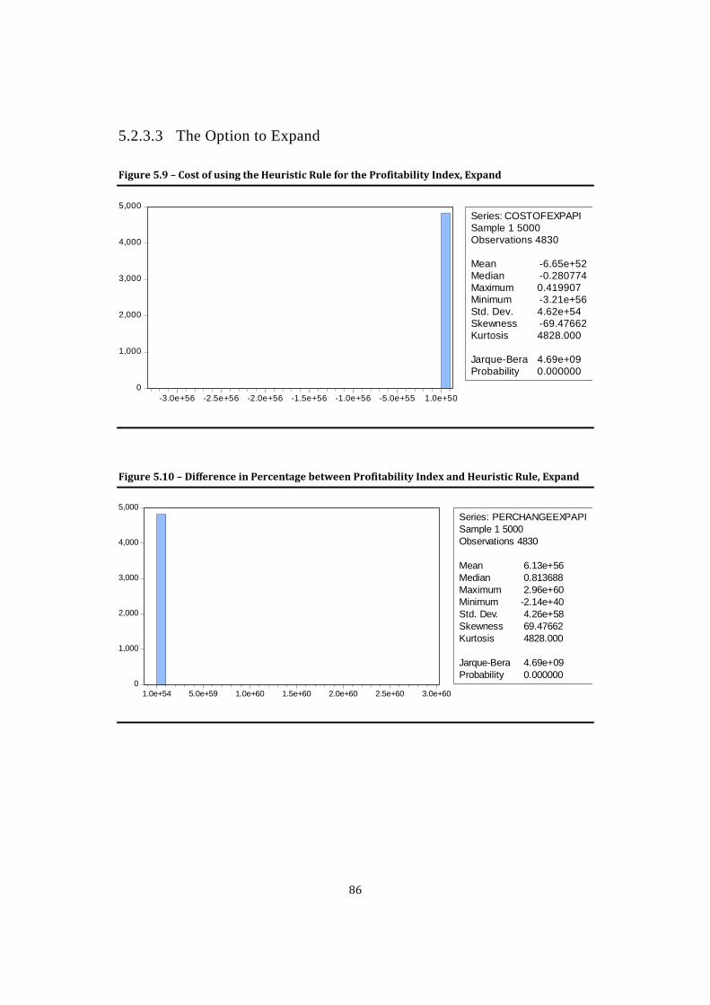
86

5.2.3.3 The Option to Expand

Figure 5.9 – Cost of using the Heuristic Rule for the Profitability Index, Expand

0

1,000

2,000

3,000

4,000

5,000

-3.0e+56 -2.5e+56 -2.0e+56 -1.5e+56 -1.0e+56 -5.0e+55 1.0e+50

Series: COSTOFEXPAPI

Sample 1 5000

Observations 4830

Mean -6.65e+52

Median -0.280774

Maximum 0.419907

Minimum -3.21e+56

Std. Dev. 4.62e+54

Skewness -69.47662

Kurtosis 4828.000

Jarque-Bera 4.69e+09

Probability 0.000000

Figure 5.10 – Difference in Percentage between Profitability Index and Heuristic Rule, Expand

0

1,000

2,000

3,000

4,000

5,000

1.0e+54 5.0e+59 1.0e+60 1.5e+60 2.0e+60 2.5e+60 3.0e+60

Series: PERCHANGEEXPAPI

Sample 1 5000

Observations 4830

Mean 6.13e+56

Median 0.813688

Maximum 2.96e+60

Minimum -2.14e+40

Std. Dev. 4.26e+58

Skewness 69.47662

Kurtosis 4828.000

Jarque-Bera 4.69e+09

Probability 0.000000

87

The heuristic for estimating the profitability index for an expansion option, are

based in a model with an explanatory power of only 50 %. Just as in the heuristic

rule for the hurdle rate, this gives rather high cost of using

Due to circumcise the profitability index will in some examples be smaller than one.

This is happening when the amount of extra capacity is relatively cheap and the

option should be exercised even though the investment is higher than the future

NPV. This example happens only in theory, as it is very rare one will expand an

investment with a profitability index below 1.

There are some problems when we are using this model. As the trigger point gets

lower, the value of the option will raise exponential, why very low numbers will

have very high values and error estimations of the trigger point, will result in very

different results and very high costs. This is very clear to see through our standard

deviation of 4.62e+54.

When we see the high cost of using the heuristic rule and taking the low explanatory

power into consideration, it is very clear that we have a weak model. We are

therefore failing our heuristic model and will not use it.

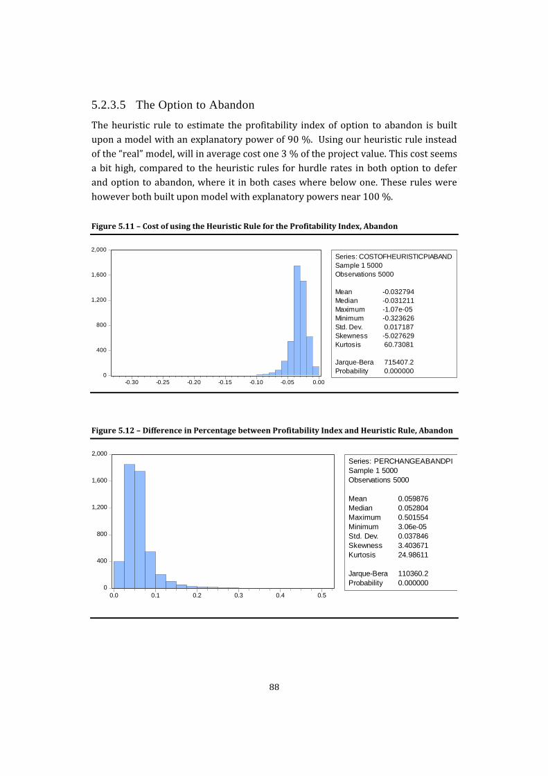
88

5.2.3.5 The Option to Abandon

The heuristic rule to estimate the profitability index of option to abandon is built

upon a model with an explanatory power of 90 %. Using our heuristic rule instead

of the “real” model, will in average cost one 3 % of the project value. This cost seems

a bit high, compared to the heuristic rules for hurdle rates in both option to defer

and option to abandon, where it in both cases where below one. These rules were

however both built upon model with explanatory powers near 100 %.

Figure 5.11 – Cost of using the Heuristic Rule for the Profitability Index, Abandon

0

400

800

1,200

1,600

2,000

-0.30 -0.25 -0.20 -0.15 -0.10 -0.05 0.00

Series: COSTOFHEURISTICPIABAND

Sample 1 5000

Observations 5000

Mean -0.032794

Median -0.031211

Maximum -1.07e-05

Minimum -0.323626

Std. Dev. 0.017187

Skewness -5.027629

Kurtosis 60.73081

Jarque-Bera 715407.2

Probability 0.000000

Figure 5.12 – Difference in Percentage between Profitability Index and Heuristic Rule, Abandon

0

400

800

1,200

1,600

2,000

0.0 0.1 0.2 0.3 0.4 0.5

Series: PERCHANGEABANDPI

Sample 1 5000

Observations 5000

Mean 0.059876

Median 0.052804

Maximum 0.501554

Minimum 3.06e-05

Std. Dev. 0.037846

Skewness 3.403671

Kurtosis 24.98611

Jarque-Bera 110360.2

Probability 0.000000

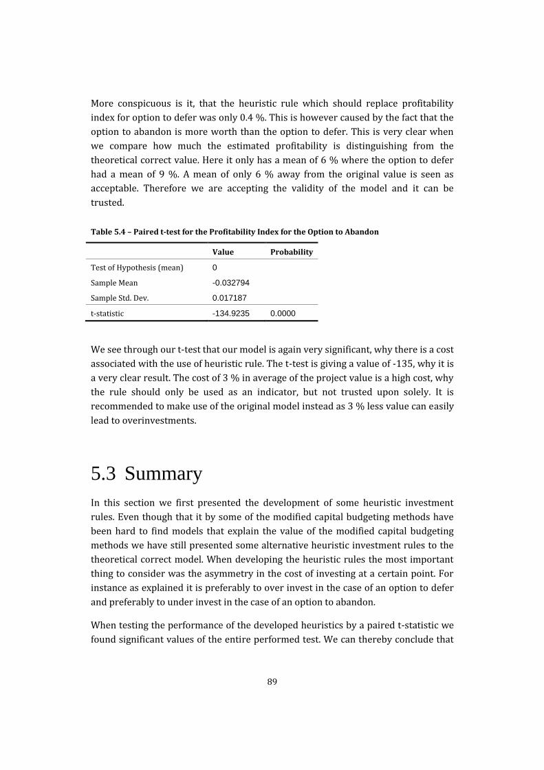
89

More conspicuous is it, that the heuristic rule which should replace profitability

index for option to defer was only 0.4 %. This is however caused by the fact that the

option to abandon is more worth than the option to defer. This is very clear when

we compare how much the estimated profitability is distinguishing from the

theoretical correct value. Here it only has a mean of 6 % where the option to defer

had a mean of 9 %. A mean of only 6 % away from the original value is seen as

acceptable. Therefore we are accepting the validity of the model and it can be

trusted.

Table 5.4 – Paired t-test for the Profitability Index for the Option to Abandon

Value Probability

Test of Hypothesis (mean) 0

Sample Mean -0.032794

Sample Std. Dev. 0.017187

t-statistic -134.9235 0.0000

We see through our t-test that our model is again very significant, why there is a cost

associated with the use of heuristic rule. The t-test is giving a value of -135, why it is

a very clear result. The cost of 3 % in average of the project value is a high cost, why

the rule should only be used as an indicator, but not trusted upon solely. It is

recommended to make use of the original model instead as 3 % less value can easily

lead to overinvestments.

5.3 Summary

In this section we first presented the development of some heuristic investment

rules. Even though that it by some of the modified capital budgeting methods have

been hard to find models that explain the value of the modified capital budgeting

methods we have still presented some alternative heuristic investment rules to the

theoretical correct model. When developing the heuristic rules the most important

thing to consider was the asymmetry in the cost of investing at a certain point. For

instance as explained it is preferably to over invest in the case of an option to defer

and preferably to under invest in the case of an option to abandon.

When testing the performance of the developed heuristics by a paired t-statistic we

found significant values of the entire performed test. We can thereby conclude that

90

using our developed heuristic investment rules has a cost compared to using the

theoretical correct model. We note although still that the percentage that our

developed heuristic investment rules are cost is relatively small, especially if the

alternative is not taking the option value into account at all.

91

6 Reflections

The research in this thesis is, due to the used theoretical frameworks and its

underlying assumptions only appropriate for proprietary investment opportunities

– in other words investment opportunities in which an individual company holds

the exclusive rights for an investment. Therefore the above developed heuristic

investment rules for the option to wait cannot with certainty be used in a business

environment in which competitors can significantly influence a given company’s

investment opportunities, for instance such as high-tech industries where first

mover advantage has a significantly role. However in other industries in which the

characteristics of the industry is more in line with the model’s assumption such as in

resource extraction industries, farming, real estate development due to the

uncertainties of the cash flow but in the same time limited competitive environment

{{155 Smit,Han T.J.,1967- 2004}}.

An important finding, and experience we have learned from in this thesis, is that the

most important objective in real options, is not to calculate the exactly correct value

or the exact optimal timing for when to exploit it. The consideration of the option

itself, is the most important objective, as the value is found through the

consideration. Even though the correct timing is not calculated, just to consider the

timing will create a value for a given company.

Other experiences which have been done throughout the thesis are the fact of

conservative thinking to choose over early entries. The asymmetric shape of the

trigger value curve, which is very steep before the peak of the curve and hereafter

more flat, makes a conservative approach favourable, hence it is more costly to

exploit a given company’s option before the peak compared to exploiting after the

peak. Here it is again important to point out, that this finding is not taking

strategically interactions into consideration. Furthermore, it was found that even

though the consideration of real options does create an extra value, the most

important factors are still found in the traditional capital budgeting methods. For

92

the option to defer the discount rate had explanatory power of 85 % and a similar

explanatory power was found for a regression only using the growth rate for the

option to abandon.

The overall purpose for the thesis, to simplify the model was only fulfilled to a

certain degree. The much complex model, where is calculated and then the

parameters should be inserted into the equation, has been substituted with simpler

equations. However some of the more abstract numbers, such as the volatility, are

still a part of the equation. Due to complexity, which often demand experience in a

large number of similar projects, of calculating such a number, it would have been

preferred to eliminate this parameter. As a possible solution, volatility could be

replaced with an instrument variable, which could be easier to measure. Due to

generated data, this experiment has not been attempted in thesis.

93

7 Conclusion

This thesis has investigated real option theory and its potential of being

approximated into simpler models seen from a practitioner’s point of view. The

research process has been focused on the five main questions stated in section 1.1.

In the following we provide a summary of the main findings and conclusions of our

research.

A fundamental part of the theoretical foundation of the thesis was presented section

2.4.3 in which the starting point, under the assumption of that cash flow would

follow a geometric Brownian motion, was the continuous-time model developed by

McDonald (1986). Furthermore by using this model it was assumed that a given

company did exclusively own the rights for the different investment opportunity.

The model was solved using contingent claims analysis, which only works under the

rather restrictive assumption of an efficient market. In other words the method

requires that there exist a complete or at least sufficiently market for assets so that

the return on a given project can be exactly replicated. The required rate of return

on the asset is calculated from the equilibrium in the capital markets and it is only

the risk free rate that is given exogenous.

After a thorough presentation and thereby understanding of the above continuous-

time model we could use the ideas from McDonald (2000) and build upon that to

further investigate if other types of real options could be incorporated into

conventional capital budgeting methods. We showed that as it was possible to

incorporate the option to defer so was it to incorporate other individual options

such as the option to expand and the option to abandon in conventional capital

budgeting methods.

In order to develop the modified capital budgeting methods into heuristic that easily

can be used of practitioners we evaluated the improved capital budgeting methods

first of all, by a sensitivity analysis of the different parameters included in the model.

94

The sensitivity analysis was enlightening in the sense of understanding how the

different parameters in the model affect the result and in relation to the

development of heuristics, which parameters had no or at least little, influence on

the models results. Moreover to get a thorough understanding of the parameters in

the model a regression analysis was carried out on various models. When we

develop the modified capital budgeting methods further the asymmetric in the cost

of investing in a certain point is considered. For instance it is preferable to over

invest in the case of an option to defer and preferably to under invest in the case of

an option to abandon. Moreover it was the objective to develop some simple models

but at the same time as accurate as possible. This trade-off arises one important

issue, which is the discussing of how reasonable accurate the developed models

should be in order to work as good enough estimates for the theoretical correct

value of the real option.

Finally, comparing the performance of the theoretical correct model for real option

valuation in a continuous-time setting with the developed heuristic investment rules

reveals that none of the developed heuristic investment rules valuate the investment

option as optimal as the theoretical correct value. We can thereby conclude that

using the developed heuristic rules has a cost compared to the "correct" value. It is

however important to note, that for both the option to defer and option to abandon,

we found some heuristic rules, with a very low cost associated, with the use of these.

The percentage cost of using these developed investment rules are relatively small.

Moreover if the alternative is not taking the option value into account we believe

that the developed heuristics can serve as good approximations, which is reasonable

accurate but not accounted for in the conventional NPV-rule. This could also be the

reason why that quite negative responds towards real option valuation in different

surveys - simply because companies are aware of such investment options

embedded in different projects and therefore takes approximations of real option

value implicitly by the use of a modified hurdle rate.

Bibliography

Arezki, R., Lederman, D. & Zhao, H. 2014, "The relative volatility of commodity

prices: a reappraisal", American Journal of Agricultural Economics, vol. 96,

no. 3, pp. 939.

Arnold, G.C. & Hatzopoulos, P.D. 2000, "The Theory-Practice Gap in Capital

Budgeting: Evidence from the United Kingdom", Journal of Business

Finance & Accounting, vol. 27, no. 5-6, pp. 603.

Berger, P.G., Ofek, E. & Swary, I. 1996, "Investor valuation of the abandonment

option", Journal of Financial Economics, vol. 42, no. 2, pp. 257.

Berk, J.,1962- & DeMarzo, P. 2011, Corporate finance, 2. global edition edn,

Pearson, Boston, MA.

Borison, A. 2005, "Real Options Analysis: Where Are the Emperor's Clothes?",

Journal of Applied Corporate Finance, vol. 17, no. 2, pp. 17.

Busby, J.S. & Pitts, C.G.C. 1997, "Real options in practice: an exploratory survey

of how finance officers deal with flexibility in capital appraisal",

Management Accounting Research, vol. 8, no. 2, pp. 169-186.

Copeland, T.E. & Antikarov, V. 2005, "Real Options: Meeting the Georgetown

Challange", Journal of Applied Corporate Finance, vol. 17, no. 2, pp. 32.

Damodaran, A. 2000, "THE PROMISE OF REAL OPTIONS", Journal of

Applied Corporate Finance, vol. 13, no. 2, pp. 29.

Dixit, A.K. 1992, "Investment and hysteresis", The journal of economic

perspectives, vol. 6, no. 1, pp. 107.

Dixit, A.K. & Pindyck, R.S. 1994, Investment under uncertainty, Princeton

University Press, Princeton, N.J.

Ingersoll, J.,Jonathan E. & Ross, S.A. 1992, "Waiting to Invest: Investment and

Uncertainty", Journal of Business, vol. 65, no. 1, pp. 1.

Kanniainen, J. 2009, "Can properly discounted projects follow geometric

Brownian motion?", Mathematical methods of operations research, vol. 70,

no. 3, pp. 435.

Kodukula, P. & Papudesu, C. 2006, Project valuation using real options : a

practitioner's guide, J. Ross Publishing, Ft. Lauderdale, Fla.

Koller, T., Goedhart, M.H., Wessels, D., Copeland, T.E.,1946- & McKinsey and

Company 2010a, Valuation : measuring and managing the value of

companies, 5. ed. edn, John Wiley & Sons, Inc., Hoboken, N.J.

Koller, T., Goedhart, M.H., Wessels, D., Copeland, T.E.,1946- & McKinsey and

Company 2010b, Valuation : measuring and managing the value of

companies, 5. ed. edn, John Wiley & Sons, Inc., Hoboken, N.J.

MacDonald, R.L. 1986, "The value of waiting to invest", The quarterly journal of

economics, vol. 101, no. 4, pp. 707.

McDonald, R.L. 2006, "The Role of Real Options in Capital Budgeting: Theory

and Practice", Journal of Applied Corporate Finance, vol. 18, no. 2, pp. 28.

McDonald, R.L. 2000, "Real Options and Rules of Thumb in Capital Budgeting"

in Project Flexibility, Agency, and Competition: New Developments in the

Theory and Application of Real Options, eds. M.J. Brennan & L. Trigeorgis,

Oxford University Press, New York, pp. 13-33.

Mun, J. 2002, Real options analysis : tools and techniques for valuing strategic

investments and decisions, John Wiley & Sons, New York, N.Y.

Ross, S.A. 1995, "Uses, Abuses, and Alternatives to the Net-Present-Value Rule",

Financial Management, vol. 24, no. 3, pp. 96.

Smit, H.T.J.,1967- & Trigeorgis, L. 2004, Strategic investment : real options and

games, Princeton University Press, Princeton, NJ.

Triantis, A. 2005, "Realizing the Potential of Real Options: Does Theory Meet

Practice?", Journal of Applied Corporate Finance, vol. 17, no. 2, pp. 8.

Wambach, A. 2000, "Payback criterion, hurdle rates and the gain of waiting",

International review of financial analysis, vol. 9, no. 3, pp. 247.

Appendix