real interest rate persistence: evidence and - st. louis fed

FEDERAL RESERVE BANK OF ST. LOUIS REVIEW NOVEMBER/DECEMBER 2008 609

Real Interest Rate Persistence: Evidence and Implications

Christopher J. Neely and David E. Rapach

The real interest rate plays a central role in many important financial and macroeconomic models,including the consumption-based asset pricing model, neoclassical growth model, and models ofthe monetary transmission mechanism. The authors selectively survey the empirical literature thatexamines the time-series properties of real interest rates. A key stylized fact is that postwar realinterest rates exhibit substantial persistence, shown by extended periods when the real interestrate is substantially above or below the sample mean. The finding of persistence in real interestrates is pervasive, appearing in a variety of guises in the literature. The authors discuss the impli-cations of persistence for theoretical models, illustrate existing findings with updated data, andhighlight areas for future research. (JEL C22, E21, E44, E52, E62, G12)

Federal Reserve Bank of St. Louis Review, November/December 2008, 90(6), pp. 609-41.

ines its long-run properties. This paper selectivelyreviews this literature, highlights its central find-ings, and analyzes their implications for theory.We illustrate our study with new empirical resultsbased on U.S. data. Two themes emerge from ourreview: (i) Real rates are very persistent, muchmore so than consumption growth; and (ii)researchers should seriously explore the causesof this persistence.

First, empirical studies find that real interestrates exhibit substantial persistence, shown byextended periods when postwar real interest ratesare substantially above or below the sample mean.Researchers characterize this feature of the datawith several types of models. One group of studiesuses unit root and cointegration tests to analyzewhether shocks permanently affect the real inter-est rate—that is, whether the real rate behaves likea random walk. Such studies often report evidence

T he real interest rate—an interest rateadjusted for either realized or expectedinflation—is the relative price of con-suming now rather than later.1 As such,

it is a key variable in important theoretical modelsin finance and macroeconomics, such as the con-sumption-based asset pricing model (Lucas, 1978;Breeden, 1979; Hansen and Singleton, 1982,1983), neoclassical growth model (Cass, 1965;Koopmans, 1965), models of central bank policy(Taylor, 1993), and numerous models of the mon-etary transmission mechanism.

The theoretical importance of the real interestrate has generated a sizable literature that exam-

1 Heterogeneous agents face different real interest rates, dependingon horizon, credit risk, and other factors. And inflation rates arenot unique, of course. For ease of exposition, this paper ignoressuch differences as being irrelevant to the economic inference.

Christopher J. Neely is an assistant vice president and economist at the Federal Reserve Bank of St. Louis. David E. Rapach is an associateprofessor of economics at Saint Louis University. This project was undertaken while Rapach was a visiting scholar at the Federal ReserveBank of St. Louis. The authors thank Richard Anderson, Menzie Chinn, Alan Isaac, Lutz Kilian, Miguel León-Ledesma, James Morley,Michael Owyang, Robert Rasche, Aaron Smallwood, Jack Strauss, and Mark Wohar for comments on earlier drafts and Ariel Weinberger forresearch assistance. The results reported in this paper were generated using GAUSS 6.1. Some of the GAUSS programs are based on codemade available on the Internet by Jushan Bai, Christian Kleiber, Serena Ng, Pierre Perron, Katsumi Shimotsu, and Achim Zeileis, and theauthors thank them for this assistance.

© 2008, The Federal Reserve Bank of St. Louis. The views expressed in this article are those of the author(s) and do not necessarily reflect theviews of the Federal Reserve System, the Board of Governors, or the regional Federal Reserve Banks. Articles may be reprinted, reproduced,published, distributed, displayed, and transmitted in their entirety if copyright notice, author name(s), and full citation are included. Abstracts,synopses, and other derivative works may be made only with prior written permission of the Federal Reserve Bank of St. Louis.

of unit roots, or—at a minimum—substantial per-sistence. Other studies extend standard unit rootand cointegration tests by considering whetherreal interest rates are fractionally integrated orexhibit significant nonlinear behavior, such asthreshold dynamics or nonlinear cointegration.Fractional integration tests typically indicate thatreal interest rates revert to their mean very slowly.Similarly, studies that find evidence of nonlinearbehavior in real interest rates identify regimes inwhich the real rate behaves like a unit root process.Another important group of studies reports evi-dence of structural breaks in the means of realinterest rates. Allowing for such breaks reducesthe persistence of deviations from the regime-specific means, so breaks reduce local persistence.The structural breaks themselves, however, stillproduce substantial global persistence in realinterest rates.

The empirical literature thus finds that per-sistence is pervasive. Although researchers haveused sundry approaches to model persistence,certain approaches are likely to be more usefulthan others. Comprehensive model selectionexercises are thus an important area for futureresearch, as they will illuminate the exact natureof real interest rate persistence.

The second theme of our survey is that theliterature has not adequately addressed the eco-nomic causes of persistence in real interest rates.Understanding such processes is crucial for assess-ing the relevance of different theoretical models.We discuss potential sources of persistence andargue that monetary shocks contribute to persis -tent fluctuations in real interest rates. While iden-tifying economic structure is always challenging,exploring the underlying causes of real interestrate persistence is an especially important areafor future research.

The rest of the paper is organized as follows.The next section reviews the predictions of eco-nomic and financial models for the long-runbehavior of the real interest rate. This informsour discussion of the theoretical implications ofthe empirical literature’s results. After distinguish-ing between ex ante and ex post measures of thereal interest rate, the third section reviews papersthat apply unit root, cointegration, fractional

integration, and nonlinearity tests to real interestrates. The fourth section discusses studies ofregime switching and structural breaks in realinterest rates. The fifth section considers sourcesof the persistence in the U.S. real interest rate andultimately argues that it is a monetary phenome-non. The sixth section summarizes our findings.

THEORETICAL BACKGROUNDConsumption-Based Asset Pricing Model

The canonical consumption-based asset pric-ing model of Lucas (1978), Breeden (1979), andHansen and Singleton (1982, 1983) posits a repre-sentative household that chooses a real consump-tion sequence, {ct}

�t=0, to maximize

subject to an intertemporal budget constraint,where β is a discount factor and u�ct� is an instan-taneous utility function. The first-order conditionleads to the familiar intertemporal Euler equation,

(1)

where 1 + rt is the gross one-period real interestrate (with payoff at period t + 1) and Et is the con-ditional expectation operator. Researchers oftenassume that the utility function is of the constantrelative risk aversion form, u�ct� = ct1–α/�1 – α�,where α is the coefficient of relative risk aversion.Combining this with the assumption of joint log-normality of consumption growth and the realinterest rate implies the log-linear version of thefirst-order condition given by equation (1) (Hansenand Singleton, 1982, 1983):

(2)

where ∆log�ct+1� = log�ct+1� – log�ct�, κ = log�β � +0.5σ 2, and σ 2 is the constant conditional varianceof log[β �ct+1/ct�–α�1 + rt �].

Equation (2) links the conditional expectationsof the growth rate of real per capita consumption[∆log�ct+1�] with the (net) real interest rate [log�1 + rt � ≅ rt ]. Rose (1988) argues that if equa-tion (2) is to hold, then these two series must have

βttt

u c( )=

∞∑ ,0

E u c u c rt t t tβ ′( ) ′( ) +( ){ } =+1 1 1/ ,

κ α− ( ) + +( ) =+E c E rt t t t∆log log ,1 1 0

Neely and Rapach

610 NOVEMBER/DECEMBER 2008 FEDERAL RESERVE BANK OF ST. LOUIS REVIEW

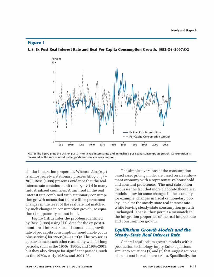
similar integration properties. Whereas ∆log�ct+1�is almost surely a stationary process [∆log�ct+1� ~I�0�], Rose (1988) presents evidence that the realinterest rate contains a unit root [rt ~ I�1�] in manyindustrialized countries. A unit root in the realinterest rate combined with stationary consump-tion growth means that there will be permanentchanges in the level of the real rate not matchedby such changes in consumption growth, so equa-tion (2) apparently cannot hold.

Figure 1 illustrates the problem identifiedby Rose (1988) using U.S. data for the ex post 3-month real interest rate and annualized growthrate of per capita consumption (nondurable goodsplus services) for 1953:Q1–2007:Q2. The two seriesappear to track each other reasonably well for longperiods, such as the 1950s, 1960s, and 1984-2001,but they also diverge for significant periods, suchas the 1970s, early 1980s, and 2001-05.

The simplest versions of the consumption-based asset pricing model are based on an endow-ment economy with a representative householdand constant preferences. The next subsectiondiscusses the fact that more elaborate theoreticalmodels allow for some changes in the economy—for example, changes in fiscal or monetary pol-icy—to alter the steady-state real interest ratewhile leaving steady-state consumption growthunchanged. That is, they permit a mismatch inthe integration properties of the real interest rateand consumption growth.

Equilibrium Growth Models and theSteady-State Real Interest Rate

General equilibrium growth models with aproduction technology imply Euler equationssimilar to equations (1) and (2) that suggest sourcesof a unit root in real interest rates. Specifically, the

Neely and Rapach


1955 1960 1965 1970 1975 1980 1985 1990 1995 2000 2005–6

–4

–2

0

2

4

6

8

10

Ex Post Real Interest Rate

Per Capita Consumption Growth

Percent

Figure 1

U.S. Ex Post Real Interest Rate and Real Per Capita Consumption Growth, 1953:Q1–2007:Q2

NOTE: The figure plots the U.S. ex post 3-month real interest rate and annualized per capita consumption growth. Consumption ismeasured as the sum of nondurable goods and services consumption.

Cass (1965) and Koopmans (1965) neoclassicalgrowth model with a representative profit-maximizing firm and utility-maximizing house-hold predicts that the steady-state real interest rateis a function of time preference, risk aversion,and the steady-state growth rate of technologicalchange (Blanchard and Fischer, 1989, Chap. 2;Barro and Sala-i-Martin, 2003, Chap. 3; Romer,2006, Chap. 2). In this model the assumption ofconstant relative risk aversion utility implies thefollowing familiar steady-state condition:

(3)

where r* is the steady-state real interest rate, ζ = –log�β � is the rate of time preference, and z isthe (expected) steady-state growth rate of labor-augmenting technological change. Equation (3)implies that a permanent change in the exogenousrate of time preference, risk aversion, or long-rungrowth rate of technology will affect the steady-state real interest rate.2 If there is no uncertainty,the neoclassical growth model implies the follow-ing steady-state version of the Euler equationgiven by (2):

(4)

where [∆log�c�]* represents the steady-stategrowth rate of ct. Substituting the right-hand sideof equation (3) into equation (4) for r*, one findsthat steady-state technology growth determinessteady-state consumption growth: [∆log�c�]* = z.

If the rate of time preference (ζ ), risk aversion(α ), and/or steady-state rate of technology growth(z) change, then (3) requires correspondingchanges in the steady-state real interest rate.Depending on the size and frequency of suchchanges, real interest rates might be very persis -tent, exhibiting unit root behavior and/or struc-tural breaks. Of these three factors, a change inthe steady-state growth rate of technology—suchas those that might be associated with the “produc-tivity slowdown” of the early 1970s and/or the“New Economy” resurgence of the mid-1990s—isthe only one that will alter both the real interestrate and consumption growth, producing non-

r z* = +ζ α ,

− − ( ) + =ζ α ∆ log ,c r* * 0

stationary behavior in both variables. Thus, itcannot explain the mismatch in the integrationproperties of the real interest rate and consump-tion growth identified by Rose (1988).

On the other hand, shocks to the preferenceparameters, ζ and α , will change only the steady-state real interest rate and not steady-state con-sumption growth. Therefore, changes inpreferences potentially disconnect the integrationproperties of real interest rates and consumptiongrowth. Researchers generally view preferencesas stable, however, making it unpalatable toascribe the persistence mismatch to such changes.3

In more elaborate models, still other factorscan change the steady-state real interest rate.For example, permanent changes in governmentpurchases and their financing can also affect thesteady-state real rate in overlapping generationsmodels with heterogeneous households(Samuelson, 1958; Diamond, 1965; Blanchard,1985; Blanchard and Fischer, 1989, Chap. 3;Romer, 2006, Chap. 2). Such shocks affect thesteady-state real interest rate without affectingsteady-state consumption growth, so they poten-tially explain the mismatch in the integrationproperties of the real interest rate and consump-tion growth examined by Rose (1988).

Finally, some monetary growth models allowfor changes in steady-state money growth to affectthe steady-state real interest rate. The seminalmodels of Mundell (1963) and Tobin (1965) pre-dict that an increase in steady-state money growthlowers the steady-state real interest rate, and morerecent micro-founded monetary models havesimilar implications (Weiss, 1980; Espinosa-Vegaand Russell, 1998a,b; Bullard and Russell, 2004;Reis, 2007; Lioui and Poncet, 2008). Again, thisclass of models permits changes in the steady-state real interest rate without correspondingchanges in consumption growth, potentiallyexplaining a mismatch in the integration proper-ties of the real interest rate and consumptiongrowth.

2 Changes in distortionary tax rates could also affect r* (Blanchardand Fischer, 1989, pp. 56-59).

Neely and Rapach


3 Some researchers appear more willing to allow for changes inpreferences over an extended period. For example, Clark (2007)argues that a steady decrease in the rate of time preference is respon-sible for the downward trend in real interest rates in Europe fromthe early medieval period to the eve of the Industrial Revolution.

Transitional Dynamics

The previous section discusses factors thatcan affect the steady-state real interest rate. Othershocks can have persistent—but ultimately tran-sitory—effects on the real rate. For example, inthe neoclassical growth model, a temporaryincrease in technology growth or governmentpurchases leads to a persistently (but not perma-nently) higher real interest rate (Romer, 2006,Chap. 2). In addition, monetary shocks can per-sistently affect the real interest rate via a varietyof frictions, such as “sticky” prices and informa-tion, adjustment costs, and learning by agentsabout policy regimes. Transient technology andfiscal shocks, as well as monetary shocks, canalso explain differences in the persistence of realinterest rates and consumption growth. For exam-ple, using a calibrated neoclassical equilibriumgrowth model, Baxter and King (1993) show thata temporary (four-year) increase in governmentpurchases persistently raises the real interest rate,although it eventually returns to its initial level.In contrast, the fiscal shock produces a much lesspersistent reaction in consumption growth. As wewill discuss later, evidence of highly persistentbut mean-reverting behavior in real interest ratessupports the empirical relevance of these shocks.

TESTING THE INTEGRATIONPROPERTIES OF REAL INTERESTRATESEx Ante versus Ex Post Real InterestRates

The ex ante real interest rate (EARR) is thenominal interest rate minus the expected inflationrate, while the ex post real rate (EPRR) is thenominal rate minus actual inflation. Agents makeeconomic decisions on the basis of their inflationexpectations over the decision horizon. For exam-ple, the Euler equations (1) and (2) relate theexpected marginal utility of consumption to theexpected real return. Therefore, the EARR is therelevant measure for evaluating economic deci-sions, and we really wish to evaluate the EARR’stime-series properties, rather than those of theEPRR.

Unfortunately, the EARR is not directly observ-able because expected inflation is not directlyobservable. An obvious solution is to use somesurvey measure of inflation expectations, suchas the Livingston Survey of professional fore-casters, which has been conducted biannuallysince the 1940s (Carlson, 1977). Economists areoften reluctant, however, to accept survey fore-casts as expectations. For example, Mishkin (1981,p. 153) expresses “serious doubts as to the qualityof these [survey] data.” Obtaining survey data atthe desired frequency for the desired sample mightcreate other obstacles to the use of survey data.Some studies have used survey data, however,including Crowder and Hoffman (1996) and Sunand Phillips (2004).

There are at least two alternative approachesto the problem of unobserved expectations. Thefirst is to use econometric forecasting methods toconstruct inflation forecasts; see, for example,Mishkin (1981, 1984) and Huizinga and Mishkin(1986). Unfortunately, econometric forecastingmodels do not necessarily include all of the rele-vant information agents use to form expectationsof inflation, and such models can fail to changewith the structure of the economy. For example,Stock and Watson (1999, 2003) show that bothreal activity and asset prices forecast inflation butthat the predictive relations change over time.4

A second alternative approach is to use theactual inflation rate as a proxy for inflation expec-tations. By definition, the actual inflation rate attime t (πt) is the sum of the expected inflation rateand a forecast error term (εt):

(5)

The literature on real interest rates has longargued that, if expectations are formed rationally,Et–1πt should be an optimal forecast of inflation(Nelson and Schwert, 1977), and εt should there-

π π εt t t tE= +−1 .

Neely and Rapach


4 Atkeson and Ohanian (2001) and Stock and Watson (2007) discussthe econometric challenges in forecasting inflation. One mightalso consider using Treasury inflation-protected securities (TIPS)yields—and/or their foreign counterparts—to measure real inter-est rates. But these series have a relatively short span of availabledata, in that the U.S. securities were first issued in 1997, are onlyavailable at long maturities (5, 10, and 20 years), and do not cor-rectly measure real rates when there is a significant chance ofdeflation.

fore be a white noise process. The EARR can beexpressed (approximately) as

(6)

where it is the nominal interest rate. Solvingequation (5) for Et�πt+1� and substituting it intoequation (6), we have

(7)

where rtep = it – πt+1 is the EPRR. Equation (7)

implies that, under rational expectations, theEPRR and EARR differ only by a white noise com-ponent, so the EPRR and EARR will share thesame long-run (integration) properties. Actually,this latter result does not require expectations tobe formed rationally but holds if the expectationerrors (εt+1) are stationary.5 Beginning with Rose(1988), much of the empirical literature tests theintegration properties of the EARR with the EPRR,after assuming that inflation-expectation errorsare stationary.

Researchers typically evaluate the integrationproperties of the EPRR with a decision rule. Theyfirst analyze the individual components of theEPRR, it and πt+1. If unit root tests indicate that itand πt+1 are both I�0�, then this implies a station-ary EPRR, as any linear combination of two I�0�processes is also an I�0� process.6 If it and πt+1have different orders of integration—for example,if it ~ I�1� and πt+1 ~ I�0�—then the EPRR musthave a unit root, as any linear combination of anI�1� process and an I�0� process is an I�1� process.Finally, if unit root tests show that it and πt+1 areboth I�1�, researchers test for a stationary EPRRby testing for cointegration between it and πt+1—that is, testing whether the linear combination

r i Etea

t t t= − +π 1,

r i

i r

tea

t t t

t t t tep

t

= − −( )= − + = +

+ +

+ + +

π ε

π ε ε1 1

1 1 1,

it – [θ0 + θ1πt+1] is a stationary process—usingone of two approaches.7 First, many researchersimpose a cointegrating vector of �1,–θ1�′ = �1,–1�′and apply unit root tests to rt

ep = it – πt+1. Thisapproach typically has more power to reject thenull of no cointegration when the true cointegrat-ing vector is �1,–1�′. The second approach is tofreely estimate the cointegrating vector betweenit and πt+1, as this allows for tax effects (Darby,1975).

If it,πt+1 ~ I�1�, then a stationary EPRR requiresit and πt+1 to be cointegrated with cointegratingcoefficient, θ1 = 1, or, allowing for tax effects, θ1 = 1/�1 – τ �, where τ is the marginal investor’smarginal tax rate on nominal interest income.When allowing for tax effects, researchers viewestimates of θ1 in the range of 1.3 to 1.4 as plausi-ble, as they correspond to a marginal tax ratearound 0.2 to 0.3 (Summers, 1983).8 It is worthemphasizing that cointegration between it andπt+1 by itself does not imply a stationary realinterest rate: θ1 must also equal 1 [or 1/�1 – τ �],as other values of θ1 imply that the equilibriumreal interest rate varies with inflation.

Although much of the empirical literatureanalyzes the EPRR in this manner, it is importantto keep in mind that the EPRR’s time-series prop-erties can differ from those of the EARR—theultimate object of analysis—in two ways. First,the EPRR’s behavior at short horizons might differfrom that of the EARR. For example, using surveydata and various econometric methods to forecastinflation, Dotsey, Lantz, and Scholl (2003) studythe behavior of the EARR and EPRR at business-cycle frequencies and find that their behaviorover the business cycle can differ significantly.Second, some estimation techniques can gener-ate different persistence properties between theEARR and EPRR; see, for example, Evans andLewis (1995) and Sun and Phillips (2004).

Early Studies

A collection of early studies on the efficientmarket hypothesis and the ability of nominal

5 Peláez (1995) provides evidence that inflation-expectation errorsare stationary. Also note that Andolfatto, Hendry, and Moran (2008)argue that inflation-expectation errors can appear serially corre-lated in finite samples, even when expectations are formed ration-ally, due to short-run learning dynamics about infrequent changesin the monetary policy regime.

6 The appendix, “Unit Roots and Cointegration Tests,” providesmore information on the mechanics of popular unit root andcointegration tests.

7 The presence of θ0 allows for a constant term in the cointegratingrelationship corresponding to the steady-state real interest rate.

Neely and Rapach


8 Data from tax-free municipal bonds would presumably provide aunitary coefficient. Crowder and Wohar (1999) study the Fishereffect with tax-free municipal bonds.

interest rates to forecast the inflation rate fore-shadows the studies that use unit root and coin-tegration tests. Fama (1975) presents evidencethat the monthly U.S. EARR can be viewed asconstant over 1953-71. Nelson and Schwert (1977),however, argue that statistical tests of Fama (1975)have low power and that his data are actually notvery informative about the EARR’s autocorrelationproperties. Hess and Bicksler (1975), Fama (1976),Carlson (1977), and Garbade and Wachtel (1978)also challenge Fama’s (1975) finding on statisticalgrounds. In addition, subsequent studies showthat Fama’s (1975) result hinges critically on theparticular sample period (Mishkin, 1981, 1984;Huizinga and Mishkin, 1986; Antoncic, 1986).

Unit Root and Cointegration Tests

The development of unit root and cointegra-tion analysis, beginning with Dickey and Fuller(1979), spurred the studies that formally test thepersistence of real interest rates. In his seminalstudy, Rose (1988) tests for unit roots in short-termnominal interest rates and inflation rates usingmonthly data for 1947-86 for 18 countries in theOrganisation for Economic Co-operation andDevelopment (OECD). Rose (1988) finds that aug-mented Dickey-Fuller (ADF) tests fail to rejectthe null hypothesis of a unit root in short-termnominal interest rates, but they can consistentlyreject a unit root in inflation rates based on vari-ous price indices—consumer price index (CPI),gross national product (GNP) deflator, implicitprice deflator, and wholesale price index (WPI).9

As discussed above, the finding that it ~ I�1�whileπt ~ I�0� indicates that the EPRR, it – πt+1, is an I�1�process. Under the assumption that inflation-expectation errors are stationary, this also impliesthat the EARR is an I�1� process. Rose (1988) eas-ily rejects the unit root null hypothesis for U.S.consumption growth, which leads him to arguethat an I�1� real interest rate and I�0� consumptiongrowth rate violates the intertemporal Euler equa-tion implied by the consumption-based asset pric-ing model. Beginning with Rose (1988), Table 1summarizes the methods and conclusions of sur-

veyed papers on the long-run properties of realinterest rates.

A number of subsequent papers also test fora unit root in real interest rates. Before estimatingstructural vector autoregressive (SVAR) models,King et al. (1991) and Galí (1992) apply ADF unitroot tests to the U.S. nominal 3-month Treasurybill rate, inflation rate, and EPRR. Using quarterlydata for 1954-88 and the GNP deflator inflationrate, King et al. (1991) fail to reject the null hypoth-esis of a unit root in the nominal interest rate,matching the finding of Rose (1988). Unlike Rose(1988), however, King et al. cannot reject the unitroot null hypothesis for the inflation rate, whichcreates the possibility that the nominal interestrate and inflation rate are cointegrated. Imposinga cointegrating vector of �1,–1�′, they fail to rejectthe unit root null hypothesis for the EPRR. Usingquarterly data for 1955-87, the CPI inflation rate,and simulated critical values that account forpotential size distortions due to moving-averagecomponents, Galí (1992) obtains unit root testresults similar to those of King et al. Despite thefailure to reject the null hypothesis that it – πt+1 ~I�1�, Galí nevertheless assumes that it – πt+1 ~ I�0�when he estimates his SVAR model, contendingthat “the assumption of a unit root in the real[interest] rate seems rather implausible on a priorigrounds, given its inconsistency with standardequilibrium growth models” (Galí, 1992, p. 717).This is in interesting contrast to King et al., whomaintain the assumption that it – πt+1 ~ I�1� in theirSVAR model. Shapiro and Watson (1988) reportsimilar unit root findings and, like Galí, stillassume the EPRR is stationary in an SVAR model.

Analyzing a 1953-90 full sample, as well as avariety of subsamples for the nominal Treasurybill rate and CPI inflation rate, Mishkin (1992)argues that monthly U.S. data are largely consis-tent with a stationary EPRR. With simulated crit-ical values, as in Galí (1992), Mishkin (1992) findsthat the nominal interest rate and inflation rateare both I�1� over four sample periods: 1953:01–1990:12, 1953:01–1979:10, 1979:11–1982:10, and1982:11–1990:12. He then tests whether the nomi-nal interest rate and inflation rate are cointegratedusing both the single-equation augmented Engleand Granger (1987, AEG) test and by prespecify-

Neely and Rapach


9 The appendix discusses unit root and cointegration tests.

Neely and Rapach


Table 1Selective Summary of the Empirical Literature on the Long-Run Properties of Real Interest Rates

Study Sample Countries Nominal interest rate and price data

Rose (1988) A: 1892-70, 1901-50 18 OECD countries Long-term corporate bond yield, short- Q: 1947-86 term commercial paper rate, GNP M: 1948-86 deflator, CPI, implicit price deflator, WPI

King et al. (1991) Q: 1949-88 U.S. 3-month U.S. Treasury bill rate, implicit GNP deflator

Galí (1992) Q: 1955-87 U.S. 3-month U.S. Treasury bill rate, CPI

Mishkin (1992) M: 1953-90 U.S. 1- and 3-month Treasury bill rates, CPI

Wallace and Warner Q: 1948-90 U.S. 3-month Treasury bill rate, 10-year (1993) government bond yield, CPI

Engsted (1995) Q: 1962-93 13 OECD countries Long-term bond yield, CPI

Mishkin and Simon Q: 1962-93 Australia 13-week government bond yield, CPI (1995)

Crowder and Hoffman Q: 1952-91 U.S. 3-month Treasury bill rate, implicit (1996) consumption deflator, Livingston

inflation expectations survey, tax data from various sources

Koustas and Serletis Q: Data begin from 11 OECD countries Various short-term nominal interest rates, (1999) 1957-72; all data CPI

end in 1995

Bierens (2000) M: 1954-94 U.S. Federal funds rate, CPI

Rapach (2003) A: Data begin in 14 industrialized countries Long-term government bond yield, 1949-65; end in implicit GDP deflator

1994-96

Rapach and Weber Q: 1957-2000 16 OECD countries Long-term government bond yield, CPI (2004)

Rapach and Wohar Q: 1960-1998 13 OECD countries Long-term government bond yield, CPI (2004) marginal tax rate data (Padovano and

Galli, 2001)

NOTE: A, Q, and M indicate annual, quarterly, and monthly data frequencies; GNP denotes gross national product.

Neely and Rapach


Results on the long-run properties of nominal interest rates, inflation rates, and real interest rates

ADF tests fail to reject a unit root for nominal interest rates but do reject for inflation rates, indicating a unit root in EPRRs. ADF tests do reject a unit root for consumption growth.

ADF tests fail to reject a unit root for the nominal interest rate, inflation rate, and EPRR.

ADF tests with simulated critical values that adjust for moving-average components fail to reject a unit root in the nominal interest rate, inflation rate, and EPRR.

ADF tests with simulated critical values that adjust for moving-average components fail to reject a unit root in the nominal interest rate and inflation rate. AEG tests typically reject the null of no cointegration, indicating a stationary EPRR.

ADF tests fail to reject a unit root in the long-term nominal interest rate and inflation rate. Johansen (1991) procedure provides evidence that the variables are cointegrated and that the EPRR is stationary.

ADF tests fail to reject a unit root in nominal interest rates and inflation rates, while cointegration tests present ambiguous results on the stationarity of the EPRR across countries.

ADF tests fail to reject a unit root in the nominal interest rate and inflation rate. AEG tests typically fail to reject the null hypothesis of no cointegration, indicating a nonstationary EPRR.

ADF test fails to reject a unit root in the nominal interest rate and inflation rate after accounting for moving-average components. Johansen (1991) procedure rejects the null of no cointegration and supports a stationary EPRR.

ADF tests usually fail to reject a unit root in nominal interest rates and inflation rates, while KPSS tests typically reject the null of stationarity, indicating nonstationary nominal interest rates and inflation rates. AEG tests typically

fail to reject the null of no cointegration, indicating a nonstationary EPRR.

New test provides evidence of nonlinear cotrending between the nominal interest rate and inflation rate, indicatinga stationary EPRR. New test, however, cannot distinguish between nonlinear cotrending and linear cointegration.

ADF tests fail to reject a unit root in all nominal interest rates and in 13 of 17 inflation rates. This indicates a nonstationary EPRR for the four countries with a stationary inflation rate. AEG tests typically fail to reject a unit

root in the EPRR for the 13 countries with a nonstationary inflation rate, indicating a nonstationary EPRR for these countries.

Ng and Perron (2001) unit root tests typically fail to reject a unit root in nominal interest rates and inflation rates. Ng and Perron (2001) and Perron and Rodriguez (2001) tests usually fail to reject the null of no cointegration, indicating a nonstationary EPRR in most countries.

Lower (upper) 95 percent confidence band for the EPRR’s ρ is close to 0.90 (above unity) for nearly every country.

Neely and Rapach


Table 1, cont’dSelective Summary of the Empirical Literature on the Long-Run Properties of Real Interest Rates


Karanasos, Sekioua, A: 1876-2000 U.S. Long-term government bond yield, CPI and Zeng (2006)

Lai (1997) Q: 1974-2001 8 industrialized and 1- to 12-month Treasury bill rates, CPI, 8 developing countries Data Resources, Inc. inflation forecasts

Tsay (2000) M: 1953-90 U.S. 1- and 3-month Treasury bill rates, CPI

Sun and Phillips (2004) Q: 1934-94 U.S. 3-month Treasury bill rate, inflation forecasts from the Survey of Professional Forecasters, CPI

Pipatchaipoom and M: 1971-2003 U.S. Eurodollar rate, CPI Smallwood (2008)

Maki (2003) M: 1972-2000 Japan 10-year bond rate, call rate, CPI

Million (2004) M: 1951-99 U.S. 3-month Treasury bill rate, CPI

Christopoulos and Q: 1960-2004 U.S. 3-month Treasury bill rate, CPI León-Ledesma (2007)

Koustas and Lamarche A: 1960-2004 G-7 countries 3-month government bill rate, CPI (2008)

Garcia and Perron (1996) Q: 1961-86 U.S. 3-month Treasury bill rate, CPI

Clemente, Montañés, Q: 1980-95 U.S., U.K. Long-term government bond yield, CPI and Reyes (1998)

Caporale and Grier (2000) Q: 1961-86 U.S. 3-month Treasury bill rate, CPI

Bai and Perron (2003) Q: 1961-86 U.S. 3-month Treasury bill rate, CPI


Neely and Rapach



95 percent confidence interval for the EPRR’s ρ is (0.97, 0.99). There is evidence of long-memory, mean-reverting behavior in the EPRR.

ADF and KPSS tests indicate a unit root in the nominal interest rate, inflation rate, and expected inflation rate. There is evidence of long-memory, mean-reverting behavior in the EARR and EPRR.

There is evidence of long-memory, mean-reverting behavior in the EPRR.

Bivariate exact Whittle estimator indicates long-memory behavior in the EARR. There is no evidence of a fractional cointegrating relationship between the nominal interest rate and expected inflation rate.

Exact Whittle estimator provides evidence of long-memory, mean-reverting behavior in the EARR.

Breitung (2002) nonparametric test that allows for nonlinear short-run dynamics provides evidence of cointegration between the nominal interest rate and inflation rate; cointegrating vector is not estimated, however, so it is not known if the cointegrating relationship is consistent with a stationary EPRR.

Luukkonen, Saikkonen, and Teräsvirta (1988) test rejects linear short-run dynamics for the adjustment to the long-run equilibrium EPRR. A smooth transition autoregressive model exhibits asymmetric mean reversion in the EPRR, depending on the level of the EPRR.

Choi and Saikkonen (2005) test provides evidence of nonlinear cointegration between the nominal interest rate and inflation rate. Exponential smooth transition regression (ESTR) model fits best over the full sample and the first

subsample (1960-78), while a logistic smooth transition regression (LSTR) model fits best over the second subsample (1979-2004). Estimated ESTR model for 1960-78 is not consistent with a stationary EPRR for any inflation rate, and estimated LSTR model for 1979–2004 is consistent with a stationary EPRR only when the inflation rate is above approximately 3 percent.

ADF and KPSS tests provide evidence of a unit root in the nominal interest rate and inflation rate. Bec, Ben Salem, and Carassco (2004) nonlinear unit root and Hansen (1996, 1997) linearity tests indicate that the EPRR can be suitably modeled as a three-regime self-exciting autoregressive (SETAR) process in Canada, France, and Italy.

An estimated autoregressive model with a three-state Markov-switching process for the mean indicates that the EPRR was in a “moderate”-mean regime for 1961-73, a “low”-mean regime for 1973-80, and a “high”-mean regime for 1980-86. EPRR is stationary with little persistence within these regimes.

ADF tests that allow for two structural breaks in the mean reject a unit root in the EPRR, indicating that the EPRR is stationary within regimes defined by structural breaks.

Bai and Perron (1998) methodology provides evidence of multiple structural breaks in the mean EPRR.

Bai and Perron (1998) methodology provides evidence of multiple structural breaks in the mean EPRR.

ing a cointegrating vector and testing for a unitroot in it – πt+1. Mishkin (1992) rejects the nullhypothesis of no cointegration for the 1953:01–1990:12 and 1953:01–1979:10 periods, but findsless frequent and weaker rejections for the1979:11–1982:10 and 1982:11–1990:12 periods.10

Mishkin and Simon (1995) apply similar tests toquarterly short-term nominal interest rate andinflation rate data for Australia. Using a 1962:Q3–1993:Q4 full sample, as well as 1962:Q3–1979:Q3and 1979:Q4– 1993:Q4 subsamples, they findevidence that both the nominal interest rate andthe inflation rate are I�1�, agreeing with the resultsfor U.S. data in Mishkin (1992). There is weakerevidence that the Australian nominal interest rateand inflation rate are cointegrated than there isfor U.S. data. Never theless, Mishkin and Simon(1995) argue that theoretical considerations war-rant viewing the long-run real interest rate as sta-tionary in Australia, as “any reasonable model ofthe macro economy would surely suggest that

real interest rates have mean-reverting tenden-cies which make them stationary” (Mishkin andSimon, 1995, p. 223).

Koustas and Serletis (1999) test for unit rootsand cointegration in short-term nominal interestrates and CPI inflation rates using quarterly datafor 1957-95 for 11 industrialized countries. Theyuse ADF unit root tests as well as the KPSS unitroot test of Kwiatkowski et al. (1992), which takesstationarity as the null hypothesis and nonstation-arity as the alternative. ADF and KPSS unit roottests indicate that it ~ I�1� and πt+1 ~ I�1� in mostcountries, so a stationary EPRR requires cointegra-tion between the nominal interest rate and infla-tion rate. Koustas and Serletis (1999), however,usually fail to find strong evidence of cointegra-tion using the AEG test. Overall, their study findsthat the EPRR is nonstationary in many industri-alized countries. Rapach (2003) obtains similarresults using postwar data for an even larger num-ber of OECD countries.

In a subtle variation on conventional cointe-gration analysis, Bierens (2000) allows an individ-ual time series to have a deterministic componentthat is a highly complex function of time—essen-tially a smooth spline—and a stationary stochasticcomponent, and he develops nonparametric pro-cedures to test whether two series share a common

10 Although they use essentially the same econometric proceduresand similar samples, Galí (1992) is unable to reject the unit rootnull hypothesis for the EPRR, while Mishkin (1992) does rejectthis null hypothesis. This illustrates the sensitivity of EPRR unitroot and cointegration tests to the specific sample. In addition,the use of short samples, such as the 1979:11–1982:10 sampleperiod considered by Mishkin (1992), is unlikely to be informativeabout the integration properties of the EPRR. To infer long-runbehavior, one needs reasonably long samples.

Neely and Rapach


Table 1, cont’dSelective Summary of the Empirical Literature on the Long-Run Properties of Real Interest Rates


Lai (2004) M: 1978-2002 U.S. 1-year Treasury bill rate, inflation expectations from the University of Michigan Survey of Consumers, CPI,federal marginal income tax rates for four-person families

Rapach and Wohar (2005) Q: 1960-98 13 OECD countries Long-term government bond yield, CPI, marginal tax rate data (Padovano and Galli, 2001)

Lai (2008) Q: 1974-2001 8 industrialized and 1- to 12-month Treasury bill rate, deposit 8 developing countries rate, CPI


deterministic component (“nonlinear cotrending”).Using monthly U.S. data for 1954-94, Bierens(2000) presents evidence that the federal fundsrate and CPI inflation rate cotrend with a vectorof �1,–1�′, which can be interpreted as evidencefor a stationary real interest rate. Bierens shows,however, that his tests cannot differentiatebetween nonlinear cotrending and linear cointe-gration in the presence of stochastic trends inthe nominal interest rate and inflation rate. Inessence, the highly complex deterministic com-ponents for the individual series closely mimicunit root behavior.

A number of studies use the Johansen (1991)system–based cointegration procedure to test fora stationary EPRR. Wallace and Warner (1993)apply the Johansen (1991) procedure to quarterlyU.S. nominal 3-month Treasury bill rate and CPIinflation data for a 1948-90 full sample and anumber of subsamples. Their results generallysupport the existence of a cointegrating relation-ship, and their estimates of θ1 are typically notsignificantly different from unity, in line with astationary EPRR. Wallace and Warner (1993) alsoargue that the expectations hypothesis impliesthat short-term and long-term nominal interestrates should be cointegrated, and they find evi-dence that U.S. short and long rates are cointe-

grated with a cointegrating vector of �1,–1�′. Inline with the results for the nominal 3-monthTreasury bill rate, Wallace and Warner find thatthe nominal 10-year Treasury bond rate and infla-tion rate are cointegrated.

With quarterly U.S. data for 1951-91, Crowderand Hoffman (1996) also use the Johansen (1991)procedure to test for cointegration between the3-month Treasury bill rate and implicit consump-tion deflator inflation rate. As in Wallace andWarner (1993), they reject the null of no cointe-gration between the nominal interest rate andinflation rate. Their estimates of θ1 range from1.22 to 1.34, which are consistent with a station-ary tax-adjusted EPRR. Crowder and Hoffman(1996) also use estimates of average marginal taxrates to directly test for cointegration betweenit�1 – τ � and πt+1. The Johansen (1991) proceduresupports cointegration and estimates a cointegrat-ing vector not significantly different from �1,–1�′,in line with a stationary tax-adjusted EPRR.

Engsted (1995) uses the Johansen (1991) pro-cedure to test for cointegration between the nomi-nal long-term government bond yield and CPIinflation rate in 13 OECD countries using quarterlydata for 1962-93. In broad agreement with theresults of Wallace and Warner (1993) and Crowderand Hoffman (1996), Engsted (1995) rejects the

Neely and Rapach



ADF tests allowing for a structural break in the mean reject a unit root in the tax-adjusted or unadjusted EARR, indicating that the EARR is stationary within regimes defined by the structural break.

The Bai and Perron (1998) methodology provides evidence of structural breaks (usually multiple) in the mean EPRR and mean inflation rate for all 13 countries.

ADF tests allowing for a structural break in the mean reject a unit root in the EPRR for most countries, indicating that the EPRR is stationary within regimes defined by the structural break.

null hypothesis of no cointegration for almost allcountries. The estimates of θ1 vary quite markedlyacross countries, however, and the values areoften inconsistent with a stationary EPRR.

Overall, unit root and cointegration testspresent mixed results with respect to the integra-tion properties of the EPRR. Generally speaking,single-equation methods provide weaker evidenceof a stationary EPRR, while the Johansen (1991)system–based approach supports a stationaryEPRR, at least for the United States. Unfortunately,econometric issues, such as the low power ofunit root tests and size distortions in the presenceof moving-average components, complicate infer-ence about persistence.

To address these econometric issues, Rapachand Weber (2004) use unit root and cointegrationtests with improved size and power. Specifically,they use the Ng and Perron (2001) unit root andPerron and Rodriguez (2001) cointegration tests.These tests incorporate aspects of the modifiedADF tests in Elliott, Rothenberg, and Stock (1996)and Perron and Ng (1996), as well as an adjustedmodified information criterion to select the auto -regressive (AR) lag order, to develop tests thatavoid size distortions while retaining power.Rapach and Weber (2004) use quarterly nominallong-term government bond yield and CPI infla-tion rate data for 1957-2000 for 16 industrializedcountries. The Ng and Perron (2001) unit root andPerron and Rodriguez (2001) cointegration testsprovide mixed results, but Rapach and Weber

interpret their results as indicating that the EPRRis nonstationary in most industrialized countriesover the postwar era.

Updated Unit Root and CointegrationTest Results for U.S. Data

Tables 2 and 3 illustrate the type of evidenceprovided by unit root and cointegration tests forthe U.S. 3-month Treasury bill rate, CPI inflationrate, and per capita consumption growth rate for1953:Q1–2007:Q2 (the same data as in Figure 1).

Table 2 reports the ADF statistic, as well asthe MZα statistic from Ng and Perron (2001), whichis designed to have better size and power proper-ties than the former. Consistent with the literature,neither test rejects the unit root null hypothesisfor the nominal interest rate. The results are mixedfor the inflation rate: The ADF statistic rejects theunit root null at the 10 percent level, but the MZαstatistic does not reject at conventional signifi-cance levels. The ADF test result that it ~ I�1�whileπt ~ I�0� means that the EPRR is nonstationary, asin Rose (1988).11 The MZα statistic’s failure toreject the unit root null for either inflation or nomi-

11 A significant moving-average component in the inflation rate couldcreate size distortions in the ADF statistic that lead us to falselyreject the unit root null hypothesis for that series. The fact that wedo not reject the unit root null using the MZα statistic—which isdesigned to avoid this size distortion—supports this interpretation.Rapach and Weber (2004), however, do reject the unit root nullfor the U.S. inflation rate using the MZα statistic and data through2000. Inflation rate unit root tests are thus particularly sensitiveto the sample period.

Neely and Rapach


Table 2Unit Root Test Statistics, U.S. data, 1953:Q1–2007:Q2

Variable ADF MZα

3-Month Treasury bill rate –2.49 [7] –4.39 [8]

PCE deflator inflation rate –2.72* [4] –5.20 [5]

Ex post real interest rate –3.06** [6] –18.83*** [2]

Per capita consumption growth –4.99*** [4] –42.07*** [2]

NOTE: The ADF and MZα statistics correspond to a one-sided (lower-tail) test of the null hypothesis that the variable has a unit rootagainst the alternative hypothesis that the variable is stationary. The 10 percent, 5 percent, and 1 percent critical values for the ADFstatistic are –2.58, –2.89, and –3.51; the 10 percent, 5 percent, and 1 percent critical values for the MZα statistic are –5.70, –8.10, and–13.80. The lag order for the regression model used to compute the test statistic is reported in brackets. *, **, and *** indicate signifi-cance at the 10 percent, 5 percent, and 1 percent levels. PCE denotes personal consumption expenditures.

nal interest rates argues for cointegration analysisof those variables to ascertain the EPRR’s integra-tion properties. When we prespecify a �1,–1�′cointegrating vector and apply unit root tests tothe EPRR, we reject the unit root null at the 5percent level using the ADF statistic and at the 1 percent level using the MZα statistic. The U.S.EPRR appears to be stationary.

To test the null hypothesis of no cointegrationwithout prespecifying a cointegrating vector,Table 3 reports the AEG statistic, MZα statisticfrom Perron and Rodriguez (2001), and trace sta-tistic from Johansen (1991). The AEG and tracestatistics reject the null hypothesis of no cointe-gration at the 10 percent level, and the MZα sta-tistic rejects the null at the 5 percent level. Table3 also reports estimates of the cointegrating coef-ficients, θ0 and θ1. Neither the dynamic ordinaryleast squares (OLS) nor Johansen (1991) estimatesof θ1 are significantly different from unity, indi-cating a stationary U.S. EPRR. The cointegratingvector is not estimated precisely enough todetermine whether there is a tax effect.

Tables 2 and 3 provide evidence that the U.S.EPRR is stationary, although some of the rejectionsare marginal. Unit root and cointegration testresults, however, are sensitive to the test proce-

dure and sample period. Studies such as Mishkin(1992), Wallace and Warner (1993), and Crowderand Hoffman (1996) find evidence of a stationaryU.S. EPRR, but Koustas and Serletis (1999) andRapach and Weber (2004) generally do not. Incontrast, per capita consumption growth is clearlystationary, as the ADF and MZα statistics in Table 2both strongly reject the unit root null hypothesisfor this variable. The fact that integration testsgive mixed results for the EPRR’s stationarity andclear-cut results for consumption growth high-lights differences in the persistence properties ofthe two variables.

Confidence Intervals for the Sum of theAutoregressive Coefficients

The sum of the AR coefficients, ρ, in the ARrepresentation of it – πt+1 equals unity for an I�1�process, while ρ < 1 for an I�0� process. It is inher-ently difficult, however, to distinguish an I�1�process from a highly persistent I�0� process, asthe two types of processes can be observationallyequivalent (Blough, 1992; Faust, 1996).12 To ana-

Neely and Rapach


12 In line with this, Crowder and Hoffman (1996) emphasize thatimpulse response analysis indicates that shocks have very persis -tent effects on the EPRR, although the U.S. EPRR appears to be I�0�.

Table 3Cointegration Test Statistics and Cointegrating Coefficient Estimates, U.S. 3-Month TreasuryBill Rate and Inflation Rate (1953:Q1–2007:Q2)

Cointegration tests

AEG MZα Trace

–3.07* [6] –17.11** [2] 19.96* [4]

Coefficient estimates

Estimation method θ0 θ1

Dynamic OLS 2.16** (1.01) 0.86*** (0.24)

Johansen (1991) maximum likelihood 0.39 (1.21) 1.44***(0.29)

NOTE: The AEG and MZα statistics correspond to a one-sided (lower-tail) test of the null hypothesis that the 3-month Treasury billrate and inflation rate are not cointegrated against the alternative hypothesis that the variables are cointegrated. The 10 percent, 5percent, and 1 percent critical values for the AEG statistic are –3.07, –3.37, and –3.96; the 10 percent, 5 percent, and 1 percent criticalvalues for the MZα statistic are –12.80, –15.84, and –22.84. The trace statistic corresponds to a one-sided (upper-tail) test of the nullhypothesis that the 3-month Treasury bill rate and inflation rate are not cointegrated against the alternative hypothesis that the vari-ables are cointegrated. The 10 percent, 5 percent, and 1 percent critical values for the trace statistic are 18.47, 20.66, and 24.18. Thelag order for the regression model used to compute the test statistic is reported in brackets. *, **, and *** indicate significance at the10 percent, 5 percent, and 1 percent levels. Standard errors are reported in parentheses.

lyze the theoretical implications of the time-seriesproperties of the real interest rate, however, wewant to determine a range of values for ρ that areconsistent with the data, not only whether ρ isless than or equal to 1. That is, a series with a ρvalue of 0.95 is highly persistent, even if it doesnot contain a unit root per se, and it is much morepersistent than a series with a ρ value of, say, 0.4.

To calculate the degree of persistence in thedata—rather than simply trying to determine ifthe series is I�0� or I�1�—Rapach and Wohar (2004)compute 95 percent confidence intervals for ρusing the Hansen (1999) grid-bootstrap andRomano and Wolf (2001) subsampling proce-dures.13 Using quarterly nominal long-term gov-ernment bond yield and CPI inflation rate datafor 13 industrialized countries for 1960-68, Rapachand Wohar (2004) report that the lower boundsof the 95 percent confidence interval for ρ for thetax-adjusted EPRR are often greater than 0.90,while the upper bounds are almost all greaterthan unity. Similarly, Karanasos, Sekioua, andZeng (2006) use a long span of monthly U.S. long-term government bond yield and CPI inflationdata for 1876-2000 to compute a 95 percent con-fidence interval for the EPRR’s ρ. Their computedinterval, (0.97, 0.99), indicates that the U.S. EPRRis a highly persistent or near-unit-root process,even if it does not actually contain a unit root.

With the same U.S. data underlying theresults in Tables 2 and 3, we use the Hansen (1999)grid-bootstrap and Romano and Wolf (2001) sub-sampling procedures to compute a 95 percentconfidence interval for ρ in the it – πt+1 process.The grid-bootstrap and subsampling confidenceintervals are (0.77, 0.97) and (0.71, 0.97), and theupper bounds are consistent with a highly persis -tent process. In contrast, the grid-bootstrap andsubsampling 95 percent confidence intervals or

ρ for per capita consumption growth are (0.34,0.70) and (0.37, 0.64). The upper bounds of theconfidence intervals for ρ for consumption growthare less than the lower bounds of the confidenceintervals for ρ for the EPRR. This is another wayto characterize the mismatch in the persistenceproperties of the EPRR and consumption growth.

Testing for Fractional Integration

Unit root and cointegration tests are designedto ascertain whether a series is I�0� or I�1�, andthe I�0�/I�1� distinction implicitly restricts—per-haps inappropriately—the types of dynamicprocesses allowed. In response, some researcherstest for fractional integration (Granger, 1980;Granger and Joyeux, 1980; Hosking, 1981) in theEARR and EPRR. A fractionally integrated seriesis denoted by I�d�, 0 ≤ d ≤ 1. When d = 0, the seriesis I�0�, and shocks die out at a geometric rate;when d = 1, the series is I�1�, and shocks havepermanent effects or “infinite memory.” An inter-mediate case occurs when 0 < d < 1: The series ismean-reverting, as in the I�0� case, but shocks nowdie out at a much slower hyperbolic (rather thangeometric) rate. Series in which 0 < d < 1 exhibit“long memory,” mean-reverting behavior, andcan be substantially more persistent than even ahighly persistent I�0� series.

A number of studies, including Lai (1997),Tsay (2000), Karanasos, Sekioua, and Zeng (2006),Sun and Phillips (2004), and Pipatchaipoom andSmallwood (2008), test for fractional integrationin the U.S. EPRR or EARR. Using U.S. postwarmonthly or quarterly U.S. data, Lai (1997), Tsay(2000), and Pipatchaipoom and Smallwood (2008)all present evidence of long-memory, mean-reverting behavior, as estimates of d for the U.S.EPRR or EARR typically range from 0.7 to 0.8 andare significantly above 0 and below 1. Using along span of annual U.S. data (1876-2000),Karanasos, Sekioua, and Zeng (2006) similarlyfind evidence of long-memory, mean-revertingbehavior in the EPRR. Sun and Phillips (2004)develop a new bivariate econometric procedurethat estimates the EARR’s d parameter in the0.75 to 1.0 range for quarterly postwar U.S. data.

Overall, fractional integration tests indicatethat the U.S. EPRR and EARR do not contain a

13 Andrews and Chen (1994) argue that the sum of the AR coefficients,ρ, characterizes the persistence in a series, as it is related to thecumulative impulse response function and the spectrum at zerofrequency. While conventional asymptotic or bootstrap confidenceintervals do not generate valid confidence intervals for nearlyintegrated processes (Basawa et al., 1991), Hansen (1999) andRomano and Wolf (2001) show that their procedures do generateconfidence intervals for ρ with correct first-order asymptotic cov-erage. Mikusheva (2007) shows, however, that while the Hansen(1999) grid-bootstrap procedure has correct asymptotical coverage,the Romano and Wolf (2001) subsampling procedure does not.

Neely and Rapach


unit root per se but are mean-reverting and verypersistent. We confirm this by estimating d for theEPRR using our sample of U.S. data for 1953:Q1–2007:Q2 with the Shimotsu (2008) semiparametrictwo-step feasible exact local Whittle estimatorthat allows for an unknown mean in the series.This estimator refines the Shimotsu and Phillips(2005) exact local Whittle estimator, and theseauthors show that such local Whittle estimatorsof d have good properties in Monte Carlo experi-ments. The estimate of d for the EPRR is 0.71, witha 95 percent confidence interval of (0.51, 0.90),so we can reject the hypothesis that d = 0 or d = 1.This evidence of long-memory, mean-revertingbehavior is consistent with the results from theliterature discussed previously. The estimate ofd for per capita consumption growth is 0.15 witha standard error of 0.10, so we cannot reject thehypothesis that d = 0 at conventional significancelevels. This is another manifestation of the dis-crepancy in persistence between the real interestrate and consumption growth.

Testing for Threshold Dynamics andNonlinear Cointegration

The empirical literature on the real interestrate typically uses models that assume both thecointegrating relationship and short-run dynamicsto be linear.14 Recently, researchers have begunto relax these linearity assumptions in favor ofnonlinear cointegration or threshold dynamics,which allow for the cointegrating relationship ormean reversion to depend on the current valuesof the variables. For example, a threshold modelmight permit the EPRR to be approximately arandom walk within ±2 percent of some long-runequilibrium value but to revert strongly to the ±2percent bands when it wanders outside thebands.15

Million (2004) presents evidence that the U.S.EPRR adjusts in a nonlinear fashion to a long-runequilibrium level using a logistic smooth transi-

tion autoregressive (LSTAR) model and monthlyU.S. 3-month Treasury bill rate and CPI inflationrate data for 1951-99. The Lagrange multipliertest of Luukkonen, Saikkonen, and Teräsvirta(1988) rejects the null hypothesis of a lineardynamic adjustment process, and there is evidenceof stronger (weaker) mean reversion in the EPRRfor values of the EPRR below (above) a thresholdlevel of 2.2 percent. Million (2004) notes that theweak mean reversion in the upper regime is con-sistent with the fact that the U.S. real interest ratewas persistently high during much of the 1980s,and he observes that the Federal Reserve’s prior-ity on fighting inflation, following the stagflationof the 1970s, could explain this period of highreal rates. In a vein similar to that of Million,Koustas and Lamarche (2008) estimate three-regime self-exciting threshold autoregressive(SETAR) models to characterize the monetarypolicy strategy of “opportunistic disinflation”(Blinder, 1994; Orphanides and Wilcox, 2002).Based on the nonlinear unit root test of Bec, Salem,and Carassco (2004) and Hansen (1996, 1997)linearity tests, Koustas and Lamarche (2008) con-clude that the EPRR can be suitably modeled asa three-regime SETAR process in Canada, France,and Italy over the postwar period.16

Christopoulos and León-Ledesma (2007)examine quarterly U.S. 3-month Treasury billrate and CPI inflation rate data for 1960-2004,permitting the cointegrating relationship itselfto be nonlinear. More precisely, they allow thecointegrating coefficient (θ1) to vary with theinflation rate by estimating logistic and smoothexponential transition regression (LSTR andESTR) models. Christopoulos and León-Ledesma(2007) find significant evidence of nonlinearcointegration between the nominal interest rateand inflation rate using the Choi and Saikkonen(2005) test. Using estimation techniques fromSaikkonen and Choi (2004), the authors conclude

Neely and Rapach


14 Studies that allow for fractional integration or structural breaksalso relax some linearity assumptions but in a different way thanthose reviewed in this subsection.

15 The purchasing power parity literature often uses these thresholdmodels (Sarno and Taylor, 2002).

16 Maki (2003) uses the Breitung (2002) nonparametric procedurethat allows for nonlinear adjustment dynamics to test for cointe-gration between the Japanese nominal interest rate and CPI infla-tion rate for 1972:01–2000:12. While Maki (2003) finds significantevidence of cointegration between the nominal interest rate andinflation rate using the Breitung (2002) test, he does not estimatethe cointegrating vector, so it is not clear that the long-run equi-librium relationship is consistent with a stationary EPRR.

that the ESTR model fits best over the full sample(1960:Q1– 2004:Q4) and the first subsample(1960:Q1–1978:Q1), whereas the LSTR modelfits best over the second subsample (1979:Q1–2004:Q4). The estimated ESTR model for 1960:Q1–1978:Q1 is not consistent with a stationary realEPRR for any inflation rate, and the estimatedLSTR model for 1979:Q1–2004:Q4 is consistentwith a stationary EPRR only when the inflationrate moves above approximately 3 percent.

In summary, recently developed econometricprocedures provide some evidence of thresholdbehavior or nonlinear cointegration in the EPRRin certain industrialized countries. In some cases,the threshold models accord well with our intu-ition about changes in central bank policies.Although evidence of threshold behavior in realinterest rates is potentially interesting, the modelsdo not obviate the persistence in real interest rates,as there are still regimes where the real interestrate behaves very much like a unit root process.

TESTING FOR REGIME SWITCHING AND STRUCTURLBREAKS IN REAL INTEREST RATES

Building on the work of Huizinga and Mishkin(1986), another strand of the empirical literaturetests for structural breaks in real interest rates.Accounting for such breaks can substantiallyreduce the persistence within the regimes definedby those breaks (Perron, 1989). Similarly, failingto account for structural breaks can produce spu-rious evidence of fractional integration (Jouiniand Nouira, 2006).

Using quarterly U.S. 3-month Treasury billrate and CPI inflation rate data for 1961-86, Garciaand Perron (1996) use Hamilton’s (1989) Markov-switching approach to test for regime shifts in theU.S. EPRR. Specifically, they allow the uncondi-tional mean of an AR(2) process to follow a three-state Markov process. The three estimated statescorrespond to high, middle, and low regimes withmeans of approximately 5.5 percent, 1.4 percent,and –1.8 percent, respectively. The filtered prob-ability estimates show that the EPRR was likelyin the middle regime from 1961-73, the low regimefrom 1973-81, and the high regime from 1981-86.

There is very little persistence within each regime,as the estimated AR coefficients (ρ1 and ρ2 inequation (A1)) are near 0 within regimes. Overall,Garcia and Perron (1996) argue that the U.S. realinterest rate occasionally experiences sizableshifts in its mean value, while the real interestrate is close to constant within the regimes.

Applications of Markov-switching modelstypically assume that the model is ergodic, so thecurrent state will eventually cycle back to anypossible state. Structural breaks have some similarproperties to Markov-switching regimes, but theyare not ergodic—they do not necessarily tend torevert to previous conditions. Because real interestrates in Garcia and Perron (1996) exhibit no obvi-ous tendency to return to previous states, struc-tural breaks might be considered more appropriatefor modeling real interest rate changes than Markovswitching. Bai and Perron (1998) develop a pow-erful methodology for testing for multiple struc-tural breaks in a regression model, and Caporaleand Grier (2000) and Bai and Perron (2003) applythis methodology to the mean of the U.S. EPRR.Both studies use quarterly U.S. short-term nominalinterest rate and CPI inflation rate data for 1961-86,and the estimated break dates are very similar:1967:Q1, 1972:Q4, and 1980:Q2 in Caporale andGrier (2000) and 1966:Q4, 1972:Q3, and 1980:Q3in Bai and Perron (2003). The breaks correspondto a decrease in the mean EPRR in 1966/1967, afurther decrease in 1972, and a sharp increase in1980. Caporale and Grier argue that changes inpolitical regimes—party control of the presidencyand Senate—produce these regime changes.

Rapach and Wohar (2005) extend the work ofCaporale and Grier (2000) and Bai and Perron(2003) by applying the Bai and Perron (1998)methodology to the EPRR in 13 industrializedcountries using tax-adjusted nominal long-termgovernment bond yield and CPI inflation rate datafor 1960-98. They find significant evidence ofstructural breaks in the mean of the EPRR in eachof the 13 countries. Rapach and Wohar (2005) alsofind that breaks in the mean inflation rate oftencoincide with breaks in the mean EPRR for eachcountry’s data. Furthermore, increases (decreases)in the mean inflation rate are almost always associ-ated with decreases (increases) in the mean EPRR.

Neely and Rapach


This finding is consistent with the hypothesisthat monetary easing increases inflation and gen-erates a persistent decline in the real interest rate.

In a comment on Rapach and Wohar (2005),Caporale and Grier (2005) examine whether politi-cal regime changes affect the mean U.S. EPRR,after controlling for the effects of regime changesin the inflation rate. Caporale and Grier (2005)find that political regime changes associated withchanges in the party of the president or controlof Congress do not affect the mean EPRR after con-trolling for inflation. However, the appointmentsof Federal Reserve Chairmen Paul Volcker in 1979and Alan Greenspan in 1987 are associated withshifts in the mean EPRR even after controllingfor changes in the mean inflation rate.

The previous papers test for structural breaksunder the assumption of stationary within-regimebehavior. In the spirit of Perron (1989), a numberof studies test whether the real interest rate is I�0�after allowing for deterministic shifts in the meanreal rate. Extending the methodology of Perronand Vogelsang (1992), Clemente, Montañés, andReyes (1998) test the unit root null hypothesis forthe U.K. and U.S. EPRR using quarterly long-termgovernment bond yield and CPI inflation rate datafor 1980-95, allowing for two breaks in the meanof the EPRR. They find that the EPRR in the UnitedKingdom and United States is an I�0� process

around an unconditional mean with two breaks.Using monthly U.S. 1-year Treasury bill rate datafor 1978-2002 and expected inflation data fromthe University of Michigan’s Survey of Consumers,Lai (2004) finds that the EARR is an I�0� processwith a shift in its unconditional mean in the early1980s. Lai (2008) extends Lai (2004) by allowingfor a mean shift in quarterly real interest rates foreight industrialized countries and eight develop-ing countries and finds widespread support for astationary EPRR after allowing for a break in theunconditional mean.

To further illustrate the prevalence of structuralbreaks, we use the Bai and Perron (1998) method-ology to test for such instability in the uncondi-tional mean of the U.S. EPRR for 1953:Q1–2007:Q2.17 Table 4 reports the results. The proce-dure finds three changes in the mean that occurat 1972:Q3, 1980:Q3, and 1989:Q3 and are similarto those previously identified for the UnitedStates.18 The breaks are associated with substan-

Neely and Rapach


17 We focus on the Bai and Perron (1998) methodology in analyzingmean real interest rate shifts in updated U.S. data. It would beinteresting in future research to consider regime-switching modelsand recently developed structural break tests such as describedby Elliott and Müller (2006).

18 Rapach and Wohar (2005) discuss how the statistics reported inTable 4 imply that there are three significant breaks in the uncon-ditional mean.

Table 4Bai and Perron (1988) Test Statistics and Estimation Results for the U.S. ex post Real InterestRate (1953:Q1–2007:Q2)

Estimated ex post Test statistic Regime real interest rate mean

UDmax 14.84*** 1953:Q1–1972:Q3 [1969:Q2, 1973:Q4] 1.22*** (0.17)

WDmax (5%) 27.06** 1972:Q4–1980:Q3 [1979:Q1, 1980:Q4] –0.55 (0.38)

F(1|0) 12.92*** 1980:Q4–1989:Q3 [1984:Q3–1994:Q2] 4.58*** (0.71)

F(2|1) 17.89*** 1989:Q4–2007:Q2 1.82*** (0.52)

F(3|2) 17.89***

F(4|3) 10.37*

F(5|4) 10.37

NOTE: *, **, and *** indicate significance at the 10 percent, 5 percent, and 1 percent levels. The bracketed dates in the Regime columndenote a 90 percent confidence interval for the end of the regime. Numbers in parentheses in the last column denote standard errorsfor the estimated mean.

tial changes in the average annualized real inter-est rate in the different regimes. The average realrate is 1.22 percent for 1953:Q1–1972:Q3, is notsignificantly different from zero for 1972:Q4–1980:Q3, increases to 4.58 percent for 1980:Q4–1989:Q3, and falls to 1.82 percent for 1989:Q4–2007:Q2. Figure 2 depicts the EPRR and the meanfor each of the four regimes defined by the threebreaks.19 In contrast to this evidence for breaksin the real rate, the Bai and Perron (1998) method-ology fails to discover significant evidence ofstructural breaks in the mean of per capita con-sumption growth. (We omit complete results forbrevity.)

In interpreting structural break results, weemphasize that such breaks only reduce within-regime or local persistence in real interest rates.The existence of breaks still implies a high degreeof global persistence, and the breaks themselvesrequire an economic explanation.

THEORETICAL IMPLICATIONSAND A MONETARY EXPLANATIONOF PERSISTENCE

This section considers what types of shocksare most likely to produce the persistence in theU.S. real interest rate. The empirical literaturedevotes relatively little attention to this importantissue. We argue that monetary shocks likely drivethe persistence in the U.S. real interest rate.

19 The test results of Bai and Perron (1998) for structural breaks in themean EPRR do not appear sensitive to whether the tax-adjusted ortax-unadjusted EPRR is used (Rapach and Wohar, 2005). Neitherdo estimates of the sum of the AR coefficients nor tests for fractionalintegration hinge critically on whether the EPRR is tax adjusted.

Neely and Rapach


1955 1960 1965 1970 1975 1980 1985 1990 1995 2000 2005–6

–4

–2

0

2

4

6

8

10

Ex Post Real Interest Rate

Regime-Specific Means

Percent

Figure 2

U.S. Ex Post Real Interest Rate and Regime-Specific Means, 1953:Q1–2007:Q2

NOTE: The figure plots the U.S. ex post real interest rate and means for the regimes defined by the structural breaks estimated usingthe Bai and Perron (1998) methodology.

Before discussing potential sources of realinterest rate persistence, we briefly make thecase that the U.S. real interest rate is ultimatelymean-reverting. As we emphasize, unit root andcointegration tests have difficulty distinguishingunit root processes from persistent but stationaryalternatives. Nevertheless, unit root and cointe-gration tests with good size and power, applied toupdated data, provide evidence that the U.S. realinterest rate is an I�0�—and thus mean-reverting—process (see Table 2).20 Tests for fractional integra-tion nest the I�0�/I�1� alternatives, and they concurthat the U.S. real interest rate is a mean-revertingprocess. Using an updated sample, we confirm thefindings of Lai (1997), Tsay (2000), Pipatchaipoomand Smallwood (2008), and Karanasos, Sekioua,and Zeng (2006) that demonstrate long-memory,mean-reverting behavior in the U.S. real interestrate. Our updated sample also provides evidenceof structural breaks in the U.S. real interest rate.Curiously, the regime-specific mean breaks for theEPRR largely cancel each other in the long run(see Table 4): The estimated mean real rate in 2007is close to that estimated for 1953.21 We specu-late that although structural breaks appear todescribe the data better than a constant, lineardata generating process, these breaks appear toexhibit a certain type of mean-reverting behavior.With sufficient data—much more than we havenow—one could presumably model this mean-reversion in regimes.

These facts lead us to tentatively claim thatthe U.S. real interest rate is best viewed as a verypersistent but ultimately mean-reverting process.We emphasize the tentative nature of this claim,and we consider careful econometric testing ofthis proposition to be an important area for futureresearch. Even if real interest rates ultimatelymean-revert, they are clearly very persistent.

Recall the underlying motivation for learningabout real interest rate persistence: In a simple

endowment economy, the real interest rate shouldhave the same persistence properties as consump-tion growth. In fact, however, real rates are muchmore persistent than consumption growth. Perma -nent technology growth shocks can create a non-stationary real rate but affect consumption growthin the same way, so they cannot account for themismatch in persistence. More complex equilib-rium growth models potentially explain this per-sistence mismatch through changing fiscal andmonetary policy, as well as transient technologygrowth shocks. We consider fiscal, monetary, andtransient technology shocks as potential causesof persistent fluctuations in the U.S. real interestrate.

Figures 1 and 2 reveal two episodes of pro-nounced and prolonged changes in the U.S. EPRR:the protracted decrease in the EPRR in the 1970sand subsequent sharp increase in the 1980s. Fiscalshocks appear to be an unlikely explanation forthe large decline in real rates from 1972-79. TheU.S. did not undertake the sort of contractionaryfiscal policy that would be necessary for such afall in real rates.22 In fact, fiscal policy in the 1970slargely tended toward modest deficits. Given thesubstantial budget deficits beginning in 1981,expansionary fiscal shocks are a more plausiblecandidate for the increase in real rates at this time.

Monetary shocks appear to fit well with theoverall pattern in the real interest rate, includingthe multiyear decline in the real rate during the1970s, the very sharp 1980 increase, and subse-quent gradual decline during the “GreatDisinflation.” One interpretation of the “GreatInflation” that began in the late 1960s and lastedthroughout the 1970s is that the Federal Reservepursued an expansionary monetary policy—eitherinadvertently or to reduce the unemployment rateto unsustainable levels—and this persistentlyreduced the real interest rate (Delong, 1997; Barskyand Kilian, 2002; Meltzer, 2005; Romer, 2005).After Paul Volcker’s appointment as Chairman,the Federal Reserve sharply raised short-termnominal interest rates to reduce inflation fromits early 1980 peak of nearly 12 percent, and this

Neely and Rapach


20 Recall, however, that unit root and cointegration tests are sensitiveto the particular sample used.

21 One might wonder if the observed mean-reversion in structuralbreaks contradicts our contention that the breaks should not bemodeled as a Markov process because they are not ergodic. We donot think, however, that observing one state twice and two statesonce provides sufficient information for a Markov process.

22 The recent analyses by Romer and Romer (2008) and Ramey (2008)indicate that the U.S. economy did not experience sizable con-tractionary fiscal policy shocks during the 1970s.

produced a sharp and prolonged increase in thereal interest rate. The structural breaks manifestthese pronounced swings: The mean EPRR fallsfrom 1.22 percent in 1972:Q3 to essentially zeroand then rises to 4.58 percent beginning in1980:Q4 (see Table 4). Furthermore, Rapach andWohar (2005) report evidence of breaks in themean U.S. inflation rate in 1973:Q1 and 1982:Q1that increase and decrease the average inflationrate. The timing and direction of the breaks areconsistent with a monetary explanation that alsoaccounts for the mismatch in persistence betweenthe real interest rate and consumption growth. Ineach case, negative (positive) breaks to the realrate of interest coincide with positive (negative)breaks in the mean rate of inflation. The data arein line with the hypothesis that central bankschange monetary policy and inflation throughpersistent effects on the real rate of interest.

Turning to technology shocks, the paucity ofindependent data on technology shocks makes it

difficult to correlate such changes with real inter-est rates. In addition, researchers have tradition-ally viewed technology growth as reasonablystable. One might think that other sorts of supplyshocks, such as oil price increases, might influencethe real rate, and they surely do to some degree;Barro and Sala-i-Martin (1990) and Caporale andGrier (2000), for example, consider this possibil-ity. It is unlikely, however, that oil price shocksalone can account for the pronounced swings inthe U.S. real interest rate: Why would rising oilprices in 1973 reduce the real interest rates butrising oil prices in 1979 dramatically raise thereal rate?23

While we interpret the timing of major swingsin the U.S. real rate to strongly suggest a mone-tary explanation, we ultimately need to estimate

23 Furthermore, Barsky and Kilian (2002) argue that the timing ofincreases in U.S. inflation in the early 1970s is more consistentwith a monetary rather than an oil price shock explanation.

Neely and Rapach


1970 1975 1980 1985 1990 1995–1.5

–1

–0.5

0

0.5

1

1.5

Figure 3

Romer and Romer (2004) Measure of Monetary Policy Shocks, 1969:Q1–1996:Q4

NOTE: A positive (negative) value corresponds to a contractionary (expansionary) monetary policy shock.

structural models to analyze the relative impor-tance of various shocks. Galí (1992) is one of thefew studies providing evidence on the economicsources of real interest rate persistence. His SVARmodel finds that an expansionary money supplyshock leads to a very persistent decline in the realinterest rate, and money supply shocks accountfor nearly 90 percent of the variance in the realrate at the one-quarter horizon and still accountfor around 60 percent of the variance at the 20-quarter horizon. Galí’s (1992) evidence is consis-tent with our monetary explanation of real interestrate persistence.24

We present tentative additional evidence insupport of a monetary explanation of real interest

rate persistence based on the new measure ofmonetary shocks developed by Romer andRomer (2004). They cull through quantitativeand narrative Federal Reserve records to computea monetary policy shock series for 1969-96 thatis independent of systematic responses to antici-pated economic conditions. Figure 3 plots theRomer and Romer (2004) monetary policy shocksseries, where expansionary (i.e., negative) shocksin the late 1960s and early 1970s and large con-tractionary (i.e., positive) shocks in the late 1970sand early 1980s appear to match well with thedecline in the U.S. real interest rate in the 1970sand subsequent sharp increase around 1980.

Romer and Romer (2004) estimate autoregres-sive distributed lag (ARDL) models to examinethe effects of a monetary policy shock on realoutput and the price level. They find that a con-tractionary shock creates persistent and sizable

Neely and Rapach


24 King and Watson (1997) and Rapach (2003) use SVAR frameworksto estimate the long-run effects of exogenous changes in inflationon the real interest rate. Both studies find evidence that an exoge-nous increase in the steady-state inflation rate decreases thesteady-state real interest rate.

0 2 4 6 8 10 12 14 16 18 20–1

0

1

2

3

4

Quarters After Shock

Percent

Figure 4

U.S. Ex Post Real Interest Rate Response to a Contractionary Romer and Romer (2004)Monetary Policy Shock

NOTE: The response is based on an autoregressive distributed lag model estimated for 1969:Q1–1996:Q4. Dashed lines delineatetwo-standard-error bands. The response is to a shock of size 0.5.

declines in both real output and the price level.In similar fashion, we estimate an ARDL model viaOLS to measure the effects of a monetary policyshock on the real interest rate. The ARDL modeltakes the form,

(8)

where rtep is the EPRR and St is the Romer and

Romer measure of monetary policy shocks.Figure 4 illustrates the response of the EPRR

to a monetary policy shock of size 0.5, which iscomparable to some of the contractionary shocksexperienced in the late 1970s and early 1980s(see Figure 3). Romer and Romer’s (2004) MonteCarlo methods provide the two-standard-errorbands. A contractionary monetary policy shockproduces a statistically and economically signif-icant increase in the U.S. EPRR, which remainsstatistically significant after approximately twoyears. Note that the response in Figure 4 is nearlyidentical to the response of rt

ep to a shock to Stobtained from a bivariate VAR(8) model that ordersSt first in a Cholesky decomposition. Together,Figures 3 and 4 show that expansionary (contrac-tionary) monetary policy shocks can account forthe pronounced and prolonged decrease (increase)in the U.S. real interest rate in the 1970s (early1980s). We emphasize that this evidence is sug-gestive. Of course, structural identification is athorny issue, and more research is needed todetermine the veracity of the monetary explana-tion for U.S. real interest rate persistence.

CONCLUSIONRose’s (1988) seminal study spurred a sizable

empirical literature that examines the time-seriesproperties of real interest rates. Our survey detailsthe evidence that real interest rates are highlypersistent. This persistence manifests itself inthe following ways:

• Under the assumption of a constant datagenerating process, many studies indicatethat real interest rates contain a unit root.While econometric problems prevent a

r a a r b S utep

j t jep

j t jj

tj

= + + +− −==∑∑0

0

8

1

8

,

dispositive resolution of this question, realinterest rates display behavior that is verypersistent, close to a unit root.

• Estimated 95 percent confidence intervalsfor the sum of the AR coefficients from theliterature have upper bounds that are greaterthan or very near unity.

• Real interest rates appear to display long-memory behavior; shocks are very long-lived, but the real interest rate is estimatedto be ultimately mean-reverting.

• Studies allowing for nonlinear dynamicsin real interest rates identify regimes wherethe real interest behaves like a unit rootprocess.

• Structural breaks in unconditional meanscharacterize real interest rates. Althoughthe breaks reduce within-regime persis -tence, the real interest rate remains highlypersistent because the regimes have differ-ent means.

Although researchers have used a variety ofeconometric models to analyze the time-seriesproperties of real interest rates, relatively littlework has been done to discriminate among thesesundry models. Model selection could tell us, forexample, whether we should think of persistentchanges in real interest rates in terms of changesin the steady-state real rate—which are consistentwith unit root behavior—or long-lived shocksthat eventually decay to a stable steady-state realrate—which are consistent with mean-revertingbehavior. While model selection raises challeng-ing econometric (and philosophical) issues, out-of-sample forecasting exercises and analysis ofposterior model probabilities in a Bayesian con-text might identify the best way to model realinterest rate persistence.

Finally, structural analysis is necessary toidentify the sources of the persistence in realinterest rates. Theoretical models suggest that avariety of shocks can induce real rate persistence,including preference, technology growth, fiscal,and monetary shocks. We suggest a tentativemonetary explanation of U.S. real interest ratepersistence based on timing, lack of persistencein consumption growth, and large and persistent

Neely and Rapach


real interest rate responses to a Romer and Romer(2004) monetary policy shock. The literaturewould greatly benefit from further analysis of therelative importance of different types of shocksin explaining real interest rate persistence.

REFERENCESAndolfatto, David; Hendry, Scott and Moran, Kevin.“Are Inflation Expectations Rational?” Journal ofMonetary Economics, March 2008, 55(2), pp. 406-22.

Andrews, Donald W.K. and Chen, Hong-Yuan.“Approximately Median-Unbiased Estimation ofAutoregressive Models.” Journal of Business andEconomic Statistics, April 1994, 12(2), pp. 187-204.

Antoncic, Madelyn. “High and Volatile Real InterestRates: Where Does the Fed Fit In?” Journal ofMoney, Credit, and Banking, February 1986, 18(1),pp. 18-27.

Atkeson, Andrew and Ohanian, Lee E. “Are PhillipsCurves Useful for Forecasting Inflation?” FederalReserve Bank of Minneapolis Quarterly Review,Winter 2001, 25(1), pp. 2-11.

Bai, Jushan and Perron, Pierre. “Estimating andTesting Linear Models with Multiple StructuralChanges.” Econometrica, 1998, 66(1), pp. 47-78.

Bai, Jushan and Perron, Pierre. “Computation andAnalysis of Multiple Structural Change Models.”Journal of Applied Econometrics, January 2003,18(1), pp. 1-22.

Barro, Robert J. and Sala-i-Martin, Xavier. “WorldReal Interest Rates,” in Olivier J. Blanchard andStanley Fischer, eds., NBER MacroeconomicsAnnual 1990. Cambridge, MA: MIT Press, 1990,pp. 15-61.

Barro, Robert J. and Sala-i-Martin, Xavier. EconomicGrowth. Second Edition. Cambridge, MA: MIT Press,2003.

Barsky, Robert B. and Kilian, Lutz. “Do We ReallyKnow that Oil Caused the Great Stagflation? AMonetary Alternative,” in Ben S. Bernanke and

Kenneth S. Rogoff, eds., NBER MacroeconomicsAnnual 2001. Cambridge, MA: MIT Press, 2002,pp. 137-83.

Basawa, I.V.; Mallik, A.K.; McCormick, W.P.; Reeves,J.H. and Taylor, R.L. “Bootstrapping Unstable First-Order Autoregressive Processes.” Annals ofStatistics, June 1991, 19(2), pp. 1098-101.

Baxter, Marianne and King, Robert G. “Fiscal Policyin General Equilibrium.” American EconomicReview, June 1993, 83(3), pp. 315-34.

Bec, Frédérique; Ben Salem, Mélika and Carassco,Marine. “Tests for Unit-Root versus ThresholdSpecification with an Application to the PurchasingPower Parity Relationship.” Journal of Businessand Economic Statistics, October 2004, 22(4), pp. 382-95.

Bierens, Herman J. “Nonparametric NonlinearCotrending Analysis, with an Application toInterest and Inflation in the United States.” Journalof Business and Economic Statistics, July 2000,18(3), pp. 323-37.

Blanchard, Olivier J. “Debt, Deficits, and FiniteHorizons.” Journal of Political Economy, April1985, 93(2), pp. 223-47.

Blanchard, Olivier J. and Fischer, Stanley. Lectureson Macroeconomics. Cambridge, MA: MIT Press,1989.

Blinder, Alan S. “Opening Statement of Alan S.Blinder at Confirmation Hearing Before the U.S.Senate Committee on Banking, Housing, and UrbanAffairs.” Unpublished manuscript, Board ofGovernors of the Federal Reserve System, May 1994.

Blough, Stephen R. “The Relationship BetweenPower and Level for Generic Unit Root Tests inFinite Samples.” Journal of Applied Econometrics,July-September 1992, 7(3), pp. 295-308.

Breeden, Douglas T. “An Intertemporal Asset PricingModel with Stochastic Consumption and InvestmentOpportunities.” Journal of Financial Economics,September 1979, 7(3), pp. 265-96.

Neely and Rapach


http://www.minneapolisfed.org/publications_papers/pub_display.cfm?id=853

http://www.minneapolisfed.org/publications_papers/pub_display.cfm?id=853

Breitung, Jörg. “Nonparametric Tests for Unit Rootsand Cointegration.” Journal of Econometrics,December 2002, 108(2), pp. 343-63.

Bullard, James B. and Russell, Steven H. “HowCostly Is Sustained Low Inflation for the U.S.Economy?” Federal Reserve Bank of St. LouisReview, May/June 2004, 86(3), pp. 35-67;research.stlouisfed.org/publications/review/04/05/Bullard.pdf.

Caporale, Tony and Grier, Kevin B. “Political RegimeChange and the Real Interest Rate.” Journal ofMoney, Credit, and Banking, August 2000, 32(3),pp. 320-34.

Caporale, Tony and Grier, Kevin B. “Inflation,Presidents, Fed Chairs, and Regime Changes in theU.S. Real Interest Rate.” Journal of Money, Credit,and Banking, December 2005, 37(6), pp. 1153-63.

Carlson, John A. “Short-Term Interest Rates asPredictors of Inflation: Comment.” AmericanEconomic Review, June 1977, 67(3), pp. 469-75.

Cass, David. “Optimum Growth in an AggregateModel of Capital Accumulation.” Review ofEconomic Studies, July 1965, 32(3), pp. 233-40.

Christopoulos, Dimitris K. and León-Ledesma,Miguel A. “A Long-Run Nonlinear Approach to theFisher Effect.” Journal of Money, Credit, andBanking, March-April 2007, 39(2-3), pp. 543-59.

Clark, Gregory. A Farewell to Alms: A Brief Historyof the Economic World. Princeton, NJ: PrincetonUniversity Press, 2007.

Choi, In and Saikkonen, Pentti. “Test for NonlinearCointegration.” Unpublished manuscript, HongKong University of Science and Technology andHelsinki University, 2005.

Clemente, Jesús; Montañés, Antonio and Reyes,Marcelo. “Testing for a Unit Root in Variables witha Double Change in Mean.” Economics Letters,May 1998, 59(2), pp. 175-82.

Crowder, William J. and Hoffman, Dennis L. “TheLong-Run Relationship Between Nominal Interest

Rates and Inflation: The Fisher Equation Revisited.”Journal of Money, Credit, and Banking, February1996, 28(1), pp. 102-18.

Crowder, William J. and Wohar, Mark E. “Are TaxEffects Important in the Long-Run FisherRelationship? Evidence from the Municipal BondMarket.” Journal of Finance, February 1999, 54(1),pp. 307-17.

Darby, Michael R. “The Financial and Tax Effects ofMonetary Policy on Interest Rates.” EconomicInquiry, June 1975, 13(2), pp. 266-76.

DeJong, David N.; Nankervis, John C.; Savin, N.E.and Whiteman, Charles H. “The Power Problems ofUnit Root Tests in Time Series with AutoregressiveErrors.” Journal of Econometrics, 1992, 53(1-3), pp. 323-43.

DeLong, J. Bradford. “America’s Peacetime Inflation:The 1970s,” in Christina D. Romer and David H.Romer, eds., Reducing Inflation. Chicago: Universityof Chicago Press, 1997, pp. 247-76.

Diamond, Peter A. “National Debt in a NeoclassicalGrowth Model.” American Economic Review,December 1965, 55(5), pp. 1126-50.

Dickey, David A. and Fuller, Wayne A. “Distributionof the Estimators for Autoregressive Time Serieswith a Unit Root.” Journal of the American StatisticalAssociation, June 1979, 74(366), pp. 427-31.

Dotsey, Michael; Lantz, Carl and Scholl, Brian. “TheBehavior of the Real Rate of Interest.” Journal ofMoney, Credit, and Banking, February 2003, 35(1),pp. 91-110.

Elliott, Graham and Müller, Ulrich. “Efficient Testsfor General Persistent Time Variation in RegressionCoefficients.” Review of Economic Studies, October2006, 73(4), pp. 907-40.

Elliott, Graham; Rothenberg, Thomas J. and Stock,James H. “Efficient Tests for an AutoregressiveUnit Root.” Econometrica, July 1996, 64(4), pp. 813-36.

Neely and Rapach


http://research.stlouisfed.org/publications/review/04/05/Bullard.pdf

Engle, Robert F. and Granger, Clive W.J. “Co-integra-tion and Error Correction: Representation,Estimation, and Testing.” Econometrica, March1987, 55(2), pp. 251-76.

Engsted, Tom. “Does the Long-Term Interest RatePredict Future Inflation? A Multi-Country Analysis.”Review of Economics and Statistics, February 1995,77(1), pp. 42-54.

Espinosa-Vega, Marco A. and Russell, Steven H.“Can Higher Inflation Reduce Real Interest Rates inthe Long Run?” Canadian Journal of Economics,February 1998a, 31(1), pp. 92-103.

Espinosa-Vega, Marco A. and Russell, Steven H.“The Long-Run Real Effects of Monetary Policy:Keynesian Predictions from a Neoclassical Model.”Working Paper No. 98-6, Federal Reserve Bank ofAtlanta, April 1998b; www.frbatlanta.org/filelegacydocs/wp9806.pdf.

Evans, Martin D.D. and Lewis, Karen K. “DoExpected Shifts in Inflation Affect Estimates of theLong-Run Fisher Relation?” Journal of Finance,March 1995, 50(1), pp. 225-53.

Fama, Eugene F. “Short-Term Interest Rates asPredictors of Inflation.” American EconomicReview, June 1975, 65(3), pp. 269-82.

Fama, Eugene F. “Inflation Uncertainty and ExpectedReturns on Treasury Bills.” Journal of PoliticalEconomy, June 1976, 84(3), pp. 427-48.

Faust, Jon. “Near Observational Equivalence andTheoretical Size Problems with Unit Root Tests.”Econometric Theory, October 1996, 12(4), pp. 724-31.

Galí, Jordi. “How Well Does the IS-LM Model FitPostwar U.S. Data?” Quarterly Journal of Economics,May 1992, 107(2), pp. 709-38.

Garbade, Kenneth and Wachtel, Paul. “Time Variationin the Relationship between Inflation and InterestRates.” Journal of Monetary Economics, November1978, 4(4), pp. 755-65.

Garcia, René and Perron, Pierre. “An Analysis of theReal Interest Rate Under Regime Shifts.” Review of

Economics and Statistics, February 1996, 78(1),pp. 111-25.

Granger, Clive W.J. “Long Memory Relationships andthe Aggregation of Dynamic Models.” Journal ofEconometrics, October 1980, 14(2), pp. 227-38.

Granger, Clive W.J. and Joyeux, Roselyne. “AnIntroduction to Long-Memory Time Series Modelsand Fractional Differencing.” Journal of Time SeriesAnalysis, 1980, 1, pp. 15-39.

Hamilton, James D. “A New Approach to theEconomic Analysis of Nonstationary Time Seriesand the Business Cycle.” Econometrica, March1989, 57(2), pp. 357-84.

Hamilton, James D. Time Series Analysis. Princeton,NJ: Princeton University Press, 1994.

Hansen, Bruce E. “Inference when a NuisanceParameter Is Not Identified Under the NullHypothesis.” Econometrica, March 1996, 64(2), pp. 413-30.

Hansen, Bruce E. “Inference in TAR Models.” Studiesin Nonlinear Dynamics and Econometrics, 1997,2(1), pp. 1-14.

Hansen, Bruce E. “The Grid Bootstrap and theAutoregressive Model.” Review of Economics andStatistics, November 1999, 81(4), pp. 594-607.

Hansen, Lars P. and Singleton, Kenneth J. “GeneralizedInstrumental Variables Estimation of NonlinearRational Expectations Models.” Econometrica,September 1982, 50(5), pp. 1269-86.

Hansen, Lars P. and Singleton, Kenneth J. “StochasticConsumption, Risk Aversion, and the TemporalBehavior of Asset Returns.” Journal of PoliticalEconomy, April 1983, 91(2), pp. 249-65.

Hess, Patrick J. and Bicksler, James L. “Capital AssetPrices Versus Time Series Models as Predictors ofInflation: The Expected Real Rate of Interest andMarket Efficiency.” Journal of Financial Economics,December 1975, 2(4), pp. 341-60.

Hosking, J.R.M. “Fractional Differencing.” Biometrika,April 1981, 68(1), pp. 165-76.

Neely and Rapach


Huizinga, John and Mishkin, Frederic S. “MonetaryPolicy Regime Shifts and the Unusual Behavior ofReal Interest Rates.” Carnegie-Rochester ConferenceSeries on Public Policy, 1986, 24, pp. 231-74.

Johansen, Søren. “Estimation and Hypothesis Testingof Cointegration Vectors in Gaussian VectorAutoregressive Model.” Econometrica, November1991, 59(6), pp. 1551-80.

Jouini, Jamel and Nouira, Leïla. “Mean-Shifts andLong-Memory in the U.S. Ex Post Real InterestRate.” Unpublished manuscript, GREQAM,Université de la Méditerranée, 2006.

Karanasos, M.; Sekioua, S.H. and Zeng, N. “On theOrder of Integration of Monthly US Ex-ante andEx-post Real Interest Rates: New Evidence fromOver a Century of Data.” Economics Letters, 2006,90(2), pp. 163-69.

King, Robert G.; Plosser, Charles I.; Stock, James H.and Watson, Mark W. “Stochastic Trend andEconomic Fluctuations.” American EconomicReview, September 1991, 81(4), pp. 819-40.

King, Robert G. and Watson, Mark W. “Testing Long-Run Neutrality.” Federal Reserve Bank of RichmondEconomic Quarterly, Summer 1997, 83(3), pp. 69-101;www.richmondfed.org/publications/economic_research/economic_quarterly/pdfs/summer1997/king.pdf.

Koopmans, Tjalling C. “On the Concept of OptimalEconomic Growth,” in The Economic Approach toDevelopment Planning. Amsterdam: Elsevier, 1965,pp. 225-300.

Koustas, Zisimos and Lamarche, Jean-François.“Evidence of Nonlinear Mean Reversion in theReal Interest Rate.” Applied Economics, 2008(forthcoming).

Koustas, Zisimos and Serletis, Apostolos. “On theFisher Effect.” Journal of Monetary Economics,August 1999, 44(1), pp. 105-30.

Kwiatkowski, Denis; Phillips, Peter C.B.; Schmidt,Peter and Shin, Yongcheol. “Testing the NullHypothesis of Stationarity Against the Alternativeof a Unit Root: How Sure Are We That Economic

Time Series Have a Unit Root?” Journal ofEconometrics, 1992, 54(1-3), pp. 159-78.

Lai, Kon S. “Long-Term Persistence in the RealInterest Rate: Evidence of a Fractional Unit Root.”International Journal of Finance and Economics,July 1997, 2(3), pp. 225-35.

Lai, Kon S. “On Structural Shifts and Stationarity ofthe Ex Ante Real Interest Rate.” InternationalReview of Economics and Finance, 2004, 13(2), pp. 217-28.

Lai, Kon S. “The Puzzling Unit Root in the RealInterest Rate and Its Inconsistency with IntertemporalConsumption Behavior.” Journal of InternationalMoney and Finance, February 2008, 27(1), pp. 140-55.

Lioui, Abraham and Poncet, Patrice. “Monetary Non-Neutrality in the Sidrauski Model UnderUncertainty.” Economics Letters, July 2008, 100(1),pp. 22-26.

Lucas, Robert E. “Asset Prices in an ExchangeEconomy.” Econometrica, November 1978, 46(6),pp. 1429-45.

Lütkepohl, Helmut and Saikkonen, Pentti. “OrderSelection in Testing for the Cointegrating Rank of aVAR Process,” in Robert F. Engle and Halbert White,eds., Cointegration, Causality, and Forecasting. AFestschrift in Honor of Clive W.J. Granger. Oxford:Oxford University Press, 1999, pp. 168-99.

Luukkonen, Ritva; Saikkonen, Pentti and Teräsvirta,Timo. “Testing Linearity Against Smooth TransitionAutoregressive Models.” Biometrika, September1988, 75(3), pp. 491-99.

Maki, Daiki. “Nonparametric Cointegration Analysisof the Nominal Interest Rate and Expected InflationRate.” Economics Letters, December 2003, 81(3),pp. 349-54.

Meltzer, Allan H. “Origins of the Great Inflation.”Federal Reserve Bank of St. Louis Review,March/April 2005, 87(2), pp. 145-75;research.stlouisfed.org/publications/review/05/03/part2/Meltzer.pdf.

Neely and Rapach


http://research.stlouisfed.org/publications/review/05/03/part2/Meltzer.pdf

Mikusheva, Anna. “Uniform Inference inAutoregressive Models.” Econometrica, 2007,75(5), pp. 1411-52.

Million, Nicolas. “Central Bank’s Interventions andthe Fisher Hypothesis: A Threshold CointegrationInvestigation.” Economic Modelling, December2004, 21(6), pp. 1051-64.

Mishkin, Frederic S. “The Real Rate of Interest: AnEmpirical Investigation.” Carnegie-RochesterConference Series on Public Policy, January 1981,15, pp. 151-200.

Mishkin, Frederic S. “The Real Interest Rate: AMulti-Country Empirical Study.” Canadian Journalof Economics, May 1984, 17(2), pp. 283-311.

Mishkin, Frederic S. “Is the Fisher Effect for Real? A Reexamination of the Relationship BetweenInflation and Interest Rates.” Journal of MonetaryEconomics, November 1992, 30(2), pp. 195-215.

Mishkin, Frederic S. and Simon, John. “An EmpiricalExamination of the Fisher Effect in Australia.”Economic Record, September 1995, 71(214), pp. 217-29.

Mundell, Robert. “Inflation and Real Interest.”Journal of Political Economy, June 1963, 71(3), pp. 280-83.

Nelson, Charles R. and Schwert, G. William. “Short-Term Interest Rates as Predictors of Inflation: OnTesting the Hypothesis that the Real Interest RateIs Constant.” American Economic Review, June1997, 67(3), pp. 478-86.

Ng, Serena and Perron, Pierre. “Lag Length Selectionand the Construction of Unit Root Tests with GoodSize and Power.” Econometrica, November 2001,69(6), pp. 1519-54.

Orphanides, Athanasios and Wilcox, David W. “The Opportunistic Approach to Disinflation.”International Finance, Spring 2002, 5(1), pp. 47-71.

Padovano, Fabio and Galli, Emma. “Tax Rates andEconomic Growth in the OECD Countries (1950-1999).” Economic Inquiry, January 2001, 39(1), pp. 44-57.

Peláez, Rolando F. “The Fisher Effect: Reprise.”Journal of Macroeconomics, Spring 1995, 17(2),pp. 333-46.

Perron, Pierre. “The Great Crash, the Oil Price Shockand the Unit Root Hypothesis.” Econometrica,November 1989, 57(6), pp. 1361-401.

Perron, Pierre.“Non-stationarities and Non-linearitiesin Canadian Inflation.” Economic Behavior andPolicy Choice Under Price Stability. Ottawa: Bankof Canada, 1994, pp. 235-91.

Perron, Pierre and Ng, Serena. “Useful Modificationsto Some Unit Root Tests with Dependent Errorsand Their Local Asymptotic Properties.” Review ofEconomic Studies, July 1996, 63(3), pp. 435-63.

Perron, Pierre and Rodriguez, Gabriel H. “ResidualBased Tests for Cointegration with GLS DetrendedData.” Unpublished manuscript, Boston University,2001.

Perron, Pierre and Vogelsang, Timothy J.“Nonstationarity and Level Shifts with anApplication to Purchasing Power Parity.” Journalof Business and Economic Statistics, July 1992,10(3), pp. 301-20.

Pesavento, Elena. “Analytical Evaluation of thePower of Tests for the Absence of Cointegration.”Journal of Econometrics, October 2004, 122(2), pp. 349-84.

Phillips, Peter C.B. and Hansen, Bruce E. “StatisticalInference in Instrumental Variables Regressionwith I(1) Variables.” Review of Economic Studies,January 1990, 57(1), pp. 99-125.

Phillips, Peter C.B. and Perron, Pierre. “Testing for aUnit Root in Time Series Regression.” Biometrika,June 1988, 75(2), pp. 335-46.

Pipatchaipoom, Onsurang and Smallwood, Aaron.“Persistence in the Real Interest Rate and theEffects of Calculating Expected Inflation.”Unpublished manuscript, University of Texas–Arlington, 2008.

Neely and Rapach


Ramey, Valerie A. “Identifying Government SpendingShocks: It’s All in the Timing.” Unpublished manuscript, University of California–San Diego,2008.

Rapach, David E. “International Evidence on theLong-Run Impact of Inflation.” Journal of Money,Credit, and Banking, February 2003, 35(1), pp. 23-48.

Rapach, David E. and Weber, Christian E. “Are RealInterest Rates Really Nonstationary? New Evidencefrom Tests with Good Size and Power.” Journal ofMacroeconomics, September 2004, 26(3), pp. 409-30.

Rapach, David E. and Wohar, Mark E. “ThePersistence in International Real Interest Rates.”International Journal of Finance and Economics,2004, 9(4), pp. 339-46.

Rapach, David E. and Wohar, Mark E. “RegimeChanges in International Real Interest Rates: AreThey a Monetary Phenomenon?” Journal of Money,Credit, and Banking, October 2005, 37(5), pp. 887-906.

Reis, Ricardo. “The Analytics of Monetary Non-Neutrality in the Sidrauski Model.” EconomicsLetters, January 2007, 94(1), pp. 129-35.

Romano, Joseph P. and Wolf, Michael. “SubsamplingIntervals in Autoregressive Models with LinearTime Trends.” Econometrica, September 2001,69(5), pp. 1283-314.

Romer, Christina D. “Origins of the Great Inflation:Commentary.” Federal Reserve Bank of St. LouisReview, March/April 2005, 87(2 Part 2), pp. 177-85;research.stlouisfed.org/publications/review/05/03/part2/Romer.pdf.

Romer, Christina D. and Romer, David H. “A NewMeasure of Monetary Shocks: Derivation andImplications.” American Economic Review,September 2004, 94(4), pp. 1055-84.

Romer, Christina D. and Romer, David H. “TheMacroeconomic Effects of Tax Changes: EstimatesBased on a New Measure of Fiscal Shocks.” NBERWorking Paper 12364, National Bureau of EconomicResearch, 2007; www.nber.org/papers/w13264.pdf.

Romer, David H. Advanced Macroeconomics. ThirdEdition. New York: McGraw-Hill, 2006.

Rose, Andrew K. “Is the Real Interest Rate Stable?”Journal of Finance, December 1988, 43(5), pp. 1095-112.

Said, Said E. and Dickey, David A. “Testing for UnitRoots in Autoregressive-Moving Average Models ofUnknown Order.” Biometrika, December 1984,71(3), pp. 599-607.

Saikkonen, Pentti. “Asymptotically EfficientEstimation of Cointegrating Regressions.”Econometric Theory, March 1991, 7(1), pp. 1-21.

Saikkonen, Pentti and Choi, In. “CointegratingSmooth Transition Regressions.” EconometricTheory, February 2004, 20(2), pp. 301-40.

Samuelson, Paul A. “An Exact Consumption-LoanModel of Interest with or without the SocialContrivance of Money.” Journal of PoliticalEconomy, December 1958, 66(6), pp. 467-82.

Sarno, Lucio and Taylor, Mark P. “Purchasing PowerParity and the Real Exchange Rate.” InternationalMonetary Fund Staff Papers, March 2002, 49(1),pp. 65-105.

Schwert, G. William. “Effects of Model Specificationon Tests for Unit Roots in Macroeconomic Data.”Journal of Monetary Economics, July 1987, 20(1),pp. 73-103.

Schwert, G. William. “Testing for Unit Roots: A Monte Carlo Investigation.” Journal of Businessand Economic Statistics, January 1989, 7(2), pp. 147-59.

Shapiro, Matthew D. and Watson, Joel. “Sources ofBusiness Cycle Fluctuations,” in Stanley Fischer,ed., NBER Macroeconomics Annual 1988.Cambridge, MA: The MIT Press, 1988, pp. 11-48.

Shimotsu, Katsumi. “Exact Local Whittle Estimationof Fractional Integration with an Unknown Meanand Time Trend.” Working paper, Queen’sUniversity, 2008.

Neely and Rapach


http://research.stlouisfed.org/publications/review/05/03/part2/Romer.pdf

Shimotsu, Katsumi and Phillips, Peter C.B. “ExactLocal Whittle Estimation of Fractional Integration.”Annals of Statistics, August 2005, 33(4), pp. 1890-933.

Stock, James H. and Watson, Mark W. “A SimpleEstimator of Cointegrating Vectors in Higher OrderIntegrated Systems.” Econometrica, July 1993,61(4), pp. 782-820.

Stock, James H. and Watson, Mark W. “ForecastingInflation.” Journal of Monetary Economics,October 1999, 44(2), pp. 293-335.

Stock, James H. and Watson, Mark W. “ForecastingOutput and Inflation: The Role of Asset Prices.”Journal of Economic Literature, September 2003,41(3), pp. 788-829.

Stock, James H. and Watson, Mark W. “Why Has U.S.Inflation Become Harder to Forecast?” Journal ofMoney, Credit, and Banking, October 2007, 39(1),pp. 3-33.

Summers, Lawrence H. “The Non-Adjustment ofNominal Interest Rates: A Study of the FisherEffect,” in James Tobin, ed., Symposium in Honorof Arthur Okun. Washington, DC: BrookingsInstitute, 1983, pp. 201-41.

Sun, Yixiao and Phillips, Peter C.B. “Understandingthe Fisher Equation.” Journal of AppliedEconometrics, November-December 2004, 19(7),pp. 869-86.

Taylor, John B. “Discretion versus Policy Rules inPractice.” Carnegie-Rochester Conference Series onPublic Policy, December 1993, 39, pp. 195-214.

Tobin, James. “Money and Economic Growth.”Econometrica, October 1965, 33(4), pp. 671-84.

Tsay, Wen-Jen. “Long Memory Story of the RealInterest Rate.” Economics Letters, June 2000, 67(3),pp. 325-30.

Wallace, Myles S. and Warner, John T. “The FisherEffect and the Term Structure of Interest Rates:Tests of Cointegration.” Review of Economics andStatistics, May 1993, 75(2), pp. 320-24.

Weiss, Laurence M. “The Effects of Money Supplyon Economic Welfare in the Steady State.”Econometrica, April 1980, 48(3), pp. 565-76.

Neely and Rapach


APPENDIXUnit Root and Cointegration Tests

This appendix briefly describes the basic framework for unit root and cointegration testing;Hamilton (1994) details the subject. Following Dickey and Fuller (1979) and Said and Dickey (1984),unit root tests are typically based on the autoregressive (AR) representation of a time series, which canbe written as follows:

(A1)

where et is a white noise disturbance term. When the sum of the AR coefficients in equation (A1),

equals 1, shocks to yt persist forever—yt has a unit root and thus has no tendency to revert to an uncon-ditional mean. Testing the null hypothesis that yt ~ I�1� against the alternative hypothesis that yt ~ I�0�is equivalent to testing

Researchers usually ignore the possibility that ρ > 1, since this would imply an explosive process, whichwe do not observe in the data. The t statistic on γ in the following augmented Dickey-Fuller (ADF)regression provides a convenient test statistic for the unit root null hypothesis:

(A2)

where δ = µ�1 – ρ�, γ = –�1 – ρ�, and

25

Under the null hypothesis that yt ~ I�1�, γ = 0, while γ < 0 under the alternative hypothesis that yt ~ I�0�.The t statistic on γ in equation (A2) has a nonstandard distribution, necessitating simulation methodsto obtain critical values.

Cointegration tests are closely related to unit root tests in that they ask whether any linear combi-nation of some set of I�1� processes (say, yt and xt) are stationary or cointegrated. The popular, residual-based augmented Engle and Granger (1987, AEG) procedure uses the following ordinary least squares(OLS) regression as a first step in testing the null hypothesis of no cointegration:

(A3)

The cointegrating vector, which defines the stable long-run relationship between yt and xt (if it exists),is given by �1,–θ1�′. One then runs an ADF-type unit root test—with no constant—on the regressionresiduals, ut = yt – �θ0 + θ1xt�, where θ0 and θ1 are the OLS estimates of θ0 and θ1. The AEG test statistic—the ADF test statistic from the residual regression—also has a nonstandard asymptotic distribution,which requires simulated critical values. When yt and xt are cointegrated, θ0 and θ1 are superconsistent,converging to their probability limits faster than the usual rate of

∆ ∆ ∆y y y y et t t k t k t= + + + + +− − − − −( )δ γ ρ ρ1 1 1 1 1 ,

ρ ρi jj ik= − = +∑ 1

.

y x ut t t= + +θ θ0 1 .

ρ ρjj

kjj

k

= =∑ ∑= <1 1

1 1� �versus .

ρ ρ= =∑ jj

k

1,

y y y et t k t k t− = −( ) + + −( ) +− −µ ρ µ ρ µ1 1 ,

1 T .

Neely and Rapach


25 The unit root tests developed by Phillips and Perron (1988) are closely related to ADF tests and are frequently used in the literature. We referto both ADF and Phillips and Perron (1988) tests simply as ADF tests in our discussion of the empirical literature in the text.

Endogeneity bias, however, renders conventional OLS standard errors incorrect. When yt and xt arecointegrated, fully modified OLS (FM-OLS; Phillips and Hansen, 1990) and dynamic OLS (DOLS;Saikkonen, 1991; Stock and Watson, 1993) procedures efficiently estimate θ0 and θ1 with appropriatestandard errors.

Johansen (1991) develops a cointegration test procedure based on the likelihood function of a systemof equations that simultaneously tests the null hypothesis of no cointegration and consistently andefficiently estimates the cointegrating vector (if it exists). This system-based approach is also popularin applied research and is potentially more powerful than the single-equation–based AEG approach(Pesavento, 2004).

Unit root and cointegration tests have two significant problems. First, they have low power to rejectthe null if the true model is a highly persistent but stationary process (DeJong et al., 1992). Second,moving-average components in the underlying data-generating process complicate inference from unitroot and cointegration tests. Schwert (1987, 1989) shows that ADF unit root tests can have substantialsize distortions that lead to spurious rejections of the unit root null hypothesis in the presence of asignificant moving-average component.26 Lütkepohl and Saikkonen (1999) show that such size distor-tions can also affect cointegration tests. This is potentially relevant when analyzing the EPRR, as Perronand Ng (1996) and others show that inflation rates often have sizable moving-average components.27

Neely and Rapach


26 There are two strategies for dealing with a significant moving-average component in the data-generating process when performing ADF unitroot tests: (i) include a large number of lags when estimating (A2), as an autoregressive moving average process with finite-order lag polyno-mials can be expressed as an infinite-order AR process; (ii) include the moving-average component in the data generating process when sim-ulating critical values.

27 Perron (1994) observes that the inflation rate could exhibit a substantial moving-average component if the monetary authority offsets inflationaryor disinflationary shocks away from a target price level path.

real interest rate persistence: evidence and - st. louis fed

Documents