Real Benefits of Virtual Prototyping Roger W. Pryor*, Ph.D. Pryor Knowledge Systems, Inc. *Corresponding author: 4918 Malibu Drive, Bloomfield Hills, MI 48302, rwpryor@pksez1.com Abstract: The concept of virtual prototyping can be found linked to many different keywords in the literature: modeling, look-ahead problem solving, etc. This poster paper briefly discusses the potential real benefits that can be realized through pre-build cost savings, minimization of the number of prototype builds, and post-build problem avoidance for physical prototypes and production products. Relative comparisons are made for typical costs and normal problem occurrences. Keywords: virtual prototype, model, pre-build analysis, problem avoidance, cost savings. 1. Introduction

The process of creating an innovative artifact, i.e. a new invention, typically involves several stages: concept, definition, prototype build, test, second prototype build, more testing, as needed, pre-production prototype build, etc. and the investment of from months to years of employee and management man-hours per build.

With the current availability of powerful, low-cost computers and versatile, multiphysics modeling software, the relative path length (time and dollars invested) to finished artifact creation can be significantly reduced through the adoption of a virtual prototype build phase, before the creation of the first real (built from physical materials) prototype build.

This paper presents a brief, but typical, example of the problems that may arise in such an artifact creation process. 2. Physical Artifact Prototype Basics

Much of my career has been devoted to researching, designing, patenting, and building electronic and/or electronics related artifacts. The one artifact that I conceived that is most widely known is the original electronic whiteboard [1]. That artifact, when conceived, required the prototyping of sub-systems with a variety of applied physical phenomena comprising optics, electronics, materials deposition, and mechanical structure analysis, to

name a few. As with any complex artifact, invented during an earlier time when computers and software were not as highly developed as they are currently, the only developmental methodology available to traverse the path from idea to artifact was to proceed into the laboratory, figure out the resources required, build a budget estimate, get approval (typically a multistep process), find or purchase the resources and endeavor to build a prototype.

Needless to say, the typical physical prototype requires testing. The resulting test data usually mandates that adjustments be made to the nominal specifications and component selection, due to not-totally-unexpected design concept and/or component variances.

In the cost calculations explored herein, only the differential costs between virtual and real (physical) prototype builds will be explored. It is assumed that the relative capitalization-related costs for the project hardware, not including specialized test fixtures, etc., and model-building software are comparable. It is also assumed herein that the necessary capital equipment, modeling software and skilled manpower are also readily available to implement either or both the real and virtual prototype builds. 3. Using COMSOL Multiphysics Models

The new COMSOL Multiphysics software version 4.X presents a totally revised and substantially new approach to the multiphysics model development paradigm. For clarity in presenting the underlying concepts involving the difference between real and virtual prototype builds, this paper presents the analysis using a basic 0D (zero dimension) model. The explored example focuses on the ease of using the new 0D SPICE modeling capability using the Electrical Circuit portion of the AC/DC Module of COMSOL Multiphysics software.

This Electrical Circuit example explores a sub-set of some of the primary prototype building problems that also demonstrate the principal values of virtual prototyping without delving exhaustively into the details of developing more complex demonstrative models.

4. Digital vs. Analog

Analog is defined as: “relating to or using signals or information represented by a continuously variable physical quantity such as spatial position or voltage” [2]. Whereas, digital is defined as: ”relating to or using signals or information represented by discrete values (digits) of a physical quantity, such as voltage or magnetic polarization, to represent arithmetic numbers or approximations to numbers from a continuum or logical expressions and variables” [3].

However, using a First Principle Analysis approach, fundamentally, all physical values, above the quantum-level are typically considered as continuous variables and thus, all circuitry is basically analog circuitry. For ease of control and measurement, analog quantities are now generally converted to digital quantities for the relative ease of computerized information processing.

In order to render electrical values (current, voltage, magnetic field strength, etc.) in a digital fashion, threshold levels must be defined and employed to distinguish the transition value (physical decision point) where a particular perceived voltage changes, for example, from a zero (0) into a one (1).

Once a transition level is physically defined by a threshold level, then the question becomes: “Is that perceived voltage above or below the threshold value?”. That is the basic question that needs to be answered at each and every circuit node throughout the building of every sub-circuit for both virtual and real prototypes. 5. Building the Virtual Prototype

Any artifact can either succeed or fail at each of the discrete connection points (nodes), for a given signal sequence, in a given time. Thus, the demonstrative model chosen as the example in this paper for the exploration of the above nodal threshold success or failure concept is the relatively simple AC/DC Module, Electrical Circuit SPICE model of a Resistor-Capacitor transient response (time constant) circuit. That circuit is shown in Figure 1 below.

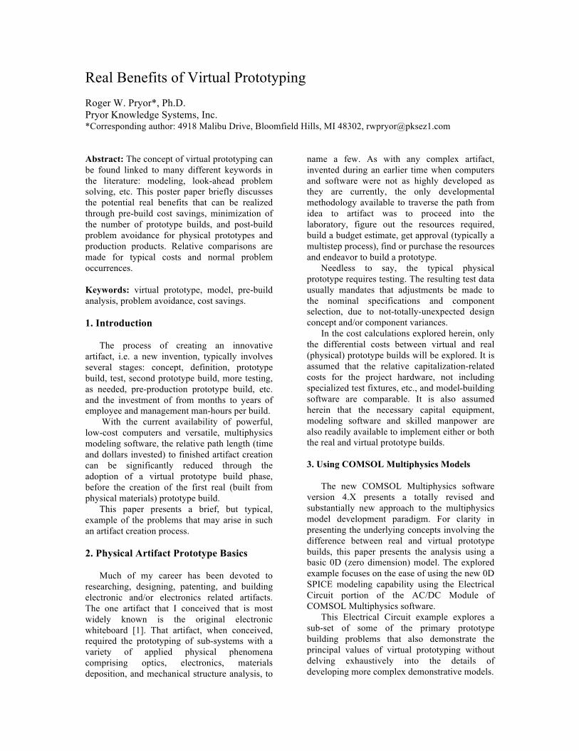
SPICE circuits are required to have at least one GROUND node. That node is designated by

the node-number zero “0”. In Figure 1, the common side of the applied voltage (V_a) and the return side of the capacitor (C_1) are both

Figure 1. Single RC Interface Node

connected at node “0”. The high side of the applied voltage (V_a) is designated node “1” and is connected to the left-end of the resistor (R_1), which has the node designation “1”. The right-end of the resistor has the node designation “2” and is connected to the supply-side of capacitor C_1, which has node designation “2”.

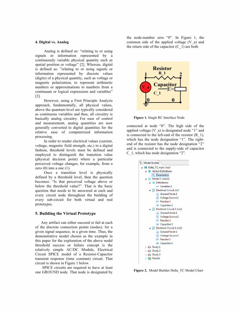
Figure 2. Model Builder Delta_TC Model Chart

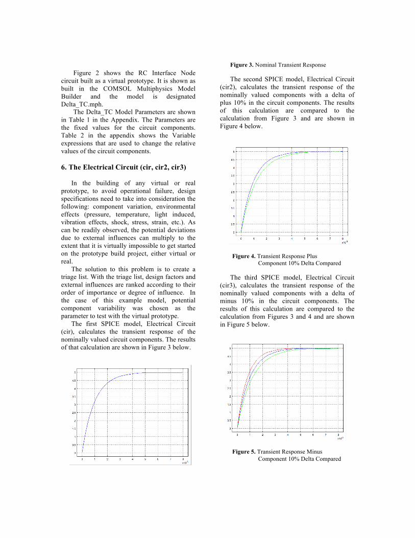
Figure 2 shows the RC Interface Node

circuit built as a virtual prototype. It is shown as built in the COMSOL Multiphysics Model Builder and the model is designated Delta_TC.mph.

The Delta_TC Model Parameters are shown in Table 1 in the Appendix. The Parameters are the fixed values for the circuit components. Table 2 in the appendix shows the Variable expressions that are used to change the relative values of the circuit components. 6. The Electrical Circuit (cir, cir2, cir3)

In the building of any virtual or real prototype, to avoid operational failure, design specifications need to take into consideration the following: component variation, environmental effects (pressure, temperature, light induced, vibration effects, shock, stress, strain, etc.). As can be readily observed, the potential deviations due to external influences can multiply to the extent that it is virtually impossible to get started on the prototype build project, either virtual or real.

The solution to this problem is to create a triage list. With the triage list, design factors and external influences are ranked according to their order of importance or degree of influence. In the case of this example model, potential component variability was chosen as the parameter to test with the virtual prototype.

The first SPICE model, Electrical Circuit (cir), calculates the transient response of the nominally valued circuit components. The results of that calculation are shown in Figure 3 below.

Figure 3. Nominal Transient Response The second SPICE model, Electrical Circuit

(cir2), calculates the transient response of the nominally valued components with a delta of plus 10% in the circuit components. The results of this calculation are compared to the calculation from Figure 3 and are shown in Figure 4 below.

Figure 4. Transient Response Plus Component 10% Delta Compared

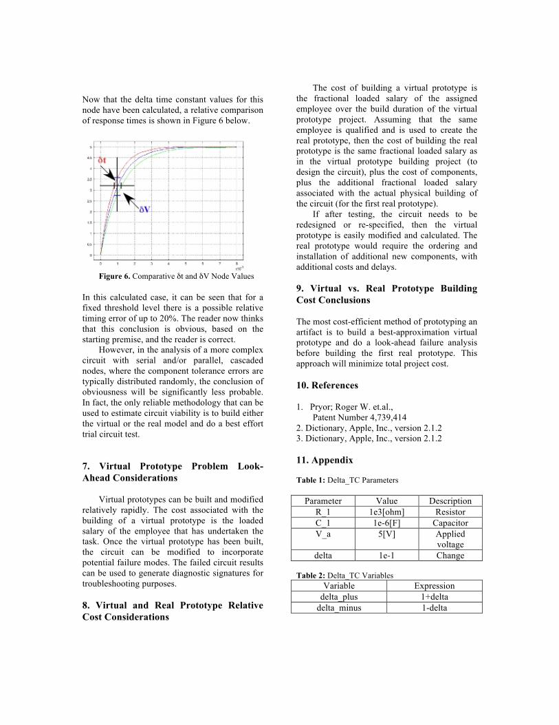
The third SPICE model, Electrical Circuit

(cir3), calculates the transient response of the nominally valued components with a delta of minus 10% in the circuit components. The results of this calculation are compared to the calculation from Figures 3 and 4 and are shown in Figure 5 below.

Figure 5. Transient Response Minus Component 10% Delta Compared

Now that the delta time constant values for this node have been calculated, a relative comparison of response times is shown in Figure 6 below.

Figure 6. Comparative δt and δV Node Values

In this calculated case, it can be seen that for a fixed threshold level there is a possible relative timing error of up to 20%. The reader now thinks that this conclusion is obvious, based on the starting premise, and the reader is correct.

However, in the analysis of a more complex circuit with serial and/or parallel, cascaded nodes, where the component tolerance errors are typically distributed randomly, the conclusion of obviousness will be significantly less probable. In fact, the only reliable methodology that can be used to estimate circuit viability is to build either the virtual or the real model and do a best effort trial circuit test.

7. Virtual Prototype Problem Look-Ahead Considerations

Virtual prototypes can be built and modified relatively rapidly. The cost associated with the building of a virtual prototype is the loaded salary of the employee that has undertaken the task. Once the virtual prototype has been built, the circuit can be modified to incorporate potential failure modes. The failed circuit results can be used to generate diagnostic signatures for troubleshooting purposes. 8. Virtual and Real Prototype Relative Cost Considerations

The cost of building a virtual prototype is the fractional loaded salary of the assigned employee over the build duration of the virtual prototype project. Assuming that the same employee is qualified and is used to create the real prototype, then the cost of building the real prototype is the same fractional loaded salary as in the virtual prototype building project (to design the circuit), plus the cost of components, plus the additional fractional loaded salary associated with the actual physical building of the circuit (for the first real prototype).

If after testing, the circuit needs to be redesigned or re-specified, then the virtual prototype is easily modified and calculated. The real prototype would require the ordering and installation of additional new components, with additional costs and delays. 9. Virtual vs. Real Prototype Building Cost Conclusions The most cost-efficient method of prototyping an artifact is to build a best-approximation virtual prototype and do a look-ahead failure analysis before building the first real prototype. This approach will minimize total project cost. 10. References 1. Pryor; Roger W. et.al.,

Patent Number 4,739,414 2. Dictionary, Apple, Inc., version 2.1.2 3. Dictionary, Apple, Inc., version 2.1.2 11. Appendix Table 1: Delta_TC Parameters

Parameter Value Description R_1 1e3[ohm] Resistor C_1 1e-6[F] Capacitor V_a 5[V] Applied

voltage delta 1e-1 Change

Table 2: Delta_TC Variables

Variable Expression delta_plus 1+delta

delta_minus 1-delta

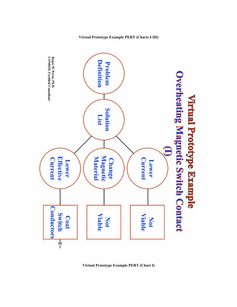
Virtual Prototype Example PERT (Charts I-III)

Virtual Prototype Example PERT (Chart I)

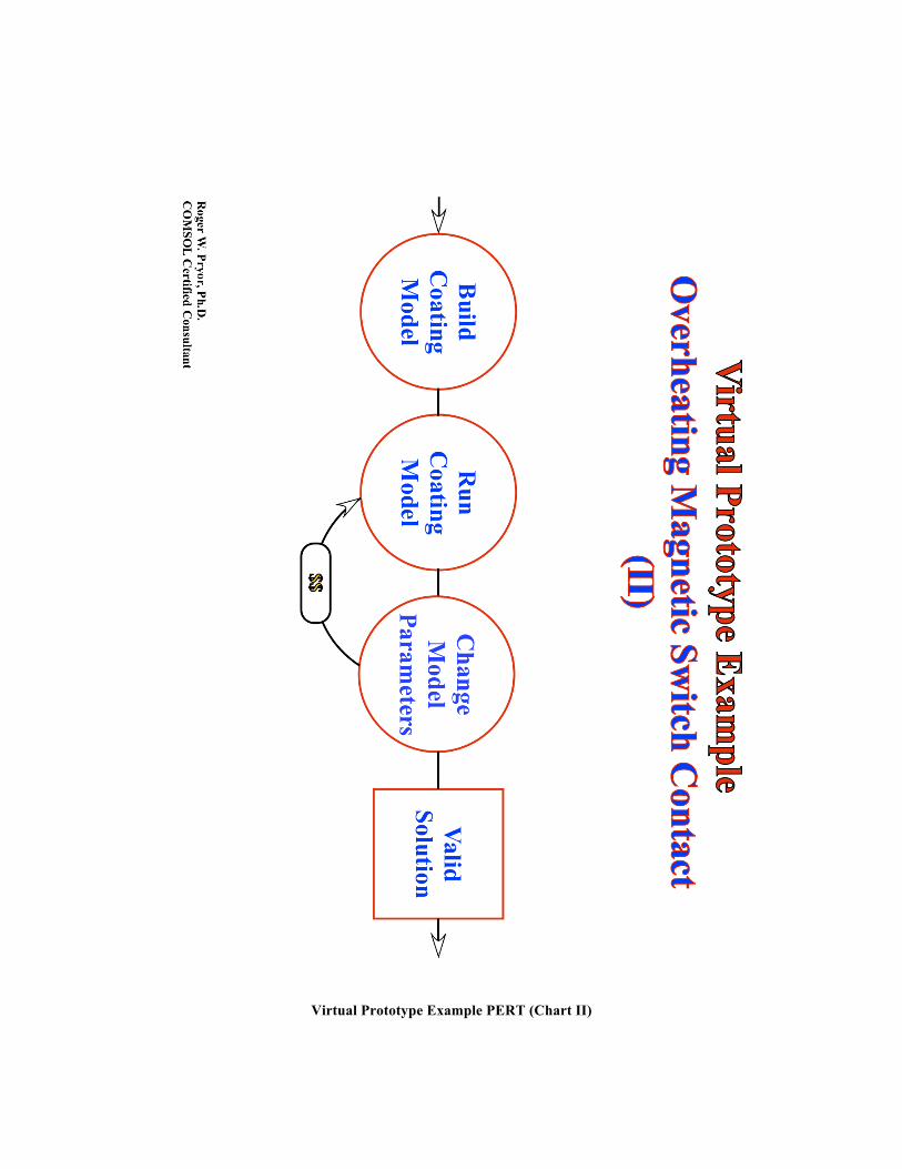
Virtual Prototype Example PERT (Chart II)

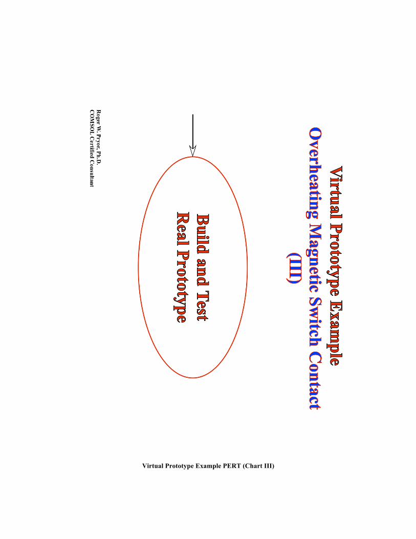
Virtual Prototype Example PERT (Chart III)

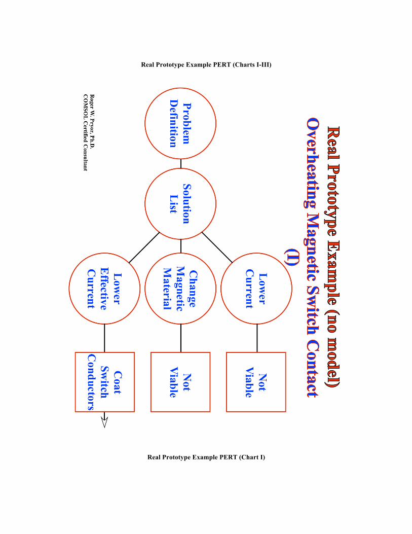
Real Prototype Example PERT (Charts I-III)

Real Prototype Example PERT (Chart I)

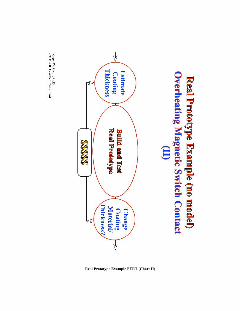
Real Prototype Example PERT (Chart II)

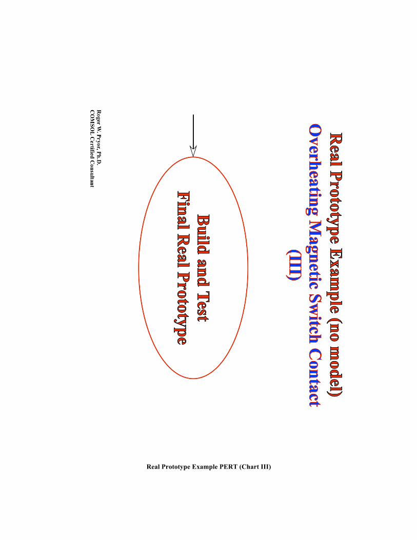
Real Prototype Example PERT (Chart III)