real analysis lecture notes: 1.4 outer measure...

REAL ANALYSIS LECTURE NOTES:

1.4 OUTER MEASURE

CHRISTOPHER HEIL

1.4.1 Introduction

We will expand on Section 1.4 of Folland’s text, which covers abstract outer measuresalso called exterior measures). To motivate the general theory, we incorporate materialfrom Chapter 3 of Wheeden and Zygmund’s text, in order to construct the fabled Lebesguemeasure on Rd. We then use this to consider abstract outer measures.

The steps in the construction of Lebesgue measure are as follows.

(a) We start with a basic class of subsets of Rd that we know how to measure, namely,cubes or rectangular boxes. We declare that their measure is their volume.

(b) We next find a way to extend the notion of measure to all subsets of Rd. For everyE ⊆ Rd we define a nonnegative, extended real-value number that we call µ∗(E)or |E|e in a way that naturally extends the notion of the volume of cubes. This isexterior Lebesgue measure. The good news is that every subset of Rd has a uniquelydefined exterior measure. The bad news is that µ∗ is not a measure — it is countablysubadditive but not countably additive.

(c) Finally, we find a way to restrict our attention to a smaller class of sets, the σ-algebraL of Lebesgue measurable subsets of Rd. We show that if µ is µ∗ restricted to this

σ-algebra, then µ is indeed a measure. This measure is Lebesgue measure on Rd.

The same idea applies more generally: If we begin with some class of subsets of X thatalready have an assigned measure, then perhaps we can extend to a subadditive outer measurethat is defined on all subsets of X, and then by restricting to some appropriate smaller σ-algebra obtain a measure on X. But first we will begin by constructing exterior Lebesguemeasure on Rd.

1.4.2 Exterior Lebesgue Measure

We begin with the familiar notion of the volume of a rectangular box in Rd, which forsimplicity we refer to as a “cube” (even though we do not require all side lengths to beequal). Other common names for such sets are intervals, rectangles, or rectangular boxes.

These notes follow and expand on the text “Real Analysis: Modern Techniques and their Applications,”

2nd ed., by G. Folland. The material on Lebesgue measure is based on the text “Measure and Integral,” by

R. L. Wheeden and A. Zygmund.

1

2 1.4 OUTER MEASURE

Definition 1. A cube in Rd is a set of the form

Q = [a1, b1]× · · · × [ad, bd] =d

∏

i=1

[ai, bi].

The volume of this cube is

vol(Q) = (b1 − a1) · · · (bd − ad) =d

∏

i=1

(bi − ai).

We extend the notion of volume to arbitrary sets by covering them with countably manycubes in all possible ways (for us, a countable set means either a finite set or a countablyinfinite set, although sometimes we repeat the phrase “finite or countably infinite” for em-phasis). For simplicity of notation, we will write {Qk}k to denote a collection of cubes Qk,with k running through some implicit index set (usually either finite or countable). Alter-natively, if we declare that the empty set is also a cube, then we can always consider a finitecollection {Qk}

Nk=1 to be an infinite collection {Qk}

∞k=1 where Qk = ∅ for k > N .

Definition 2. The exterior Lebesgue measure or outer Lebesgue measure of a set E ⊆ Rd is

|E|e = inf{

∑

k

vol(Qk)}

where the infimum is taken over all all finite or countably infinite collections of cubes Qk

such that E ⊆ ∪Qk.

We prefer to denote exterior Lebesgue measure by |E|e, though if we wanted to be moreconsistent with Folland’s notation, we should write µ∗(E) instead.

Every subset of Rd has a uniquely defined exterior measure, which lies in the range

0 ≤ |E|e ≤ ∞.

Note the following immediate, but important, consequences of the definition of exteriormeasure.

• If Qk are countably many cubes and E ⊆ ∪Qk, then |E|e ≤∑

vol(Qk).

• Given ε > 0, there exist countably many cubes Qk with E ⊆ ∪Qk such that

|E|e ≤∑

k

vol(Qk) ≤ |E|e + ε.

Note that we might have |E|e =∞ in the line above.

Example 3. Suppose that E = {x1, x2, . . . } is a countable subset of Rd, and choose anyε > 0. For each k, choose a cube Qk that contains xk and that has volume vol(Qk) < ε/2k.Then E ⊆ ∪Qk, so |E|e ≤

∑

vol(Qk) ≤ ε. Since ε is arbitrary, we conclude that |E|e = 0.Thus, every countable subset of Rd has exterior measure zero.

Next we will explore some of the properties of Lebesgue measure.

Lemma 4 (Monotonicity). If A ⊆ B ⊆ Rd, then |A|e ≤ |B|e.

1.4 OUTER MEASURE 3

Proof. If {Qk}k is any countable cover of B by cubes, then it is also a cover of A by cubes,so we have

|A|e ≤∑

k

vol(Qk).

This is true for every possible covering of B, so

|A|e ≤ inf{

∑

k

vol(Qk) : all covers of B by cubes}

= |B|e. �

The important point in proof is that if CA is the collection of all covers of A by cubes, andCB the collection of covers of B, then CB ⊆ CA. Every covering of B is a covering of A, butin general there are more ways to cover A than there are to cover B.

Exercise 5. Let C ⊆ [0, 1] ⊆ R be the classical middle-thirds Cantor set. Use monotonicityto show that the exterior Lebesgue measure of C is |C|e = 0. Thus C is an uncountablesubset of R that has exterior measure zero.

Exercise 6 (Translation Invariance). Show that if E ⊆ R and h ∈ Rd, then |E +h|e = |E|e,where E + h = {x + h : x ∈ E}.

Note that if Q is a cube, then the collection {Q} containing only the single cube Q is acovering of Q by cubes. Hence we certainly have |Q|e ≤ vol(Q). However, it requires somecare to show that the exterior measure of a cube actually coincides with its volume.

Theorem 7 (Consistency with Volume). If Q is a cube in Rd then |Q|e = vol(Q).

Proof. We have seen that |Q|e ≤ vol(Q), so we must prove the opposite inequality.Let {Qk}k be any countable covering of Q by cubes, and fix any ε > 0. For each k, let Q∗

k

be any cube such that:

• Qk is contained in the interior of Q∗k, i.e., Qk ⊆ (Q∗

k)◦, and

• vol(Q∗k) ≤ (1 + ε) vol(Qk).

Then we have

Q ⊆⋃

k

Qk ⊆⋃

k

(Q∗

k)◦.

Hence {(Q∗k)

◦} is a countable open cover of the compact set Q. It must therefore have afinite subcover, i.e., there must exist an N > 0 such that

Q ⊆N⋃

k=1

(Q∗

k)◦ ⊆

N⋃

k=1

Q∗

k.

Now, since we are dealing with cubes, we have (proof by exercise) that

vol(Q) ≤N

∑

k=1

vol(Q∗

k) ≤ (1 + ε)N

∑

k=1

vol(Qk) ≤ (1 + ε)∑

k

vol(Qk).

4 1.4 OUTER MEASURE

Since this is true for every covering {Qk}k, we conclude that

vol(Q) ≤ (1 + ε) inf{

∑

k

vol(Qk)}

= (1 + ε) |Q|e.

Since ε is arbitrary, it follows that vol(Q) ≤ |Q|e. �

We have constructed a function | · |e that is defined on every subset of Rd and has theproperties:

• 0 ≤ |E|e ≤ ∞ for every E ⊆ Rd,

• |E + h|e = |E| for every E ⊆ Rd and h ∈ Rd,

• |Q|e = vol(Q) for every cube Q.

Looking back to our very first theorem in Section 1.1, it follows that | · |e cannot possibly becountably additive, and therefore it cannot be a measure on Rd:

Exterior Lebesgue measure is not a measure on Rd.

Rather unsettlingly, there exist sets E, F ⊂ Rd such that

E ∩ F = ∅ yet |E ∪ F |e < |E|e + |F |e.

On the other hand, let us prove that exterior Lebesgue measure is at least countablysubadditive.

Theorem 8 (Countable Subadditivity). If E1, E2, . . . ⊆ Rd, then∣

∣

∣

⋃

k

Ek

∣

∣

∣

e≤

∑

k

|Ek|e.

Proof. If any Ek satisfies |Ek|e = ∞ then we are done, so let us assume that |Ek|e < ∞ for

every k. Fix any ε > 0. Then for each k we can find a covering {Q(k)j }j of Ek by cubes Q

(k)j

in such a way that∑

j

vol(Q(k)j ) ≤ |Ek|e +

ε

2k.

Then we have⋃

k

Ek ⊆⋃

k,j

Q(k)j ,

so∣

∣

∣

⋃

k

Ek

∣

∣

∣

e≤

∑

k,j

vol(Q(k)j ) ≤

∑

k

(

|Ek|e +ε

2k

)

=∑

k

|Ek|e + ε.

Since ε is arbitrary, the result follows. �

The next result states that every set E can be surrounded by an open set U whose exteriormeasure is only ε larger than that of E (by monotonicity we of course also have |E|e ≤ |U |e,so the measure of U is very close to the measure of E).

1.4 OUTER MEASURE 5

Theorem 9. If E ⊆ Rd and ε > 0, then there exists an open set U ⊇ E such that

|U |e ≤ |E|e + ε,

and hence

|E|e = inf{

|U |e : U open, U ⊇ E}

. (1)

Proof. If |E|e =∞, take U = Rd. Otherwise we have |E|e <∞, so by definition of exteriormeasure there must exist cubes Qk such that E ⊆ ∪Qk and

∑

vol(Qk) ≤ |E| +ε2. Let Q∗

k

be a larger cube that contains Qk in its interior, and such that vol(Q∗k) ≤ vol(Qk) + 2−k−1ε.

Let U be the union of the interiors of the cubes Q∗k. Then E ⊆ U , U is open, and

|U |e ≤∑

k

vol(Q∗

k) ≤∑

k

vol(Qk) +ε

2≤ |E|+ ε. �

Since E and U\E are disjoint and their union is U , we might expect that the sum oftheir exterior measures is the exterior measure of U . Unfortunately, this is false in general(although the Axiom of Choice is required to show the existence of a counterexample).Consequently, the fact that |U |e ≤ |E|e + ε does not imply that |U\E|e ≤ ε! The “well-behaved” sets for which this is true will be said to be measurable, and are studied in thenext section.

The next exercise pushes this “surrounding” issue a bit further.

Exercise 10. Show that if E ⊆ Rd, then there exists a Gδ-set H ⊇ E such that

|E|e = |H|e.

Thus, every subset E of Rd is contained in a Gδ-set H that has exactly the same exteriorLebesgue measure as E.

1.4.3 Outer Measures

Now let us use the example of exterior Lebesgue measure to see how to define more generalouter measures.

Definition 11 (Outer Measure). Let X be a nonempty set. An outer measure or exterior

measure on X is a function µ∗ : P(X)→ [0,∞] that satisfies the following conditions.

(a) µ∗(∅) = 0.

(b) Monotonicity: If A ⊆ B, then µ∗(A) ≤ µ∗(B).

(c) Countable subadditivity: If A1, A2, . . . ⊆ X, then

µ∗

(

⋃

i

Ai

)

≤∑

i

µ∗(Ai).

We want to show now that if we are given any particular class of “elementary sets” whosemeasures are specified, then we can extend this to an outer measure on X.

6 1.4 OUTER MEASURE

Theorem 12. Let E ⊆ P(X) be any fixed collection of sets such that ∅ ∈ E and there existcountably many Ek ∈ E such that ∪Ek = X (we refer to the elements of E as elementary

sets). Suppose that ρ : E → [0,∞] satisfies ρ(∅) = 0. For each A ⊆ X, define

µ∗(A) = inf{

∑

k

ρ(Ek)}

, (2)

where the infimum is taken over all finite or countable covers of A by sets Ek ∈ E . Then µ∗

is an outer measure on X.

Proof. The given hypotheses ensure that every subset of X has at least one covering byelements of E . Hence the infimum in equation (2) is not taken over the empty set, andtherefore does define a value in [0,∞] for each A ⊆ X.

Since {∅} is one covering of ∅ by elements of E , we have that

0 ≤ µ∗(∅) ≤ ρ(∅) = 0.

To show monotonicity, suppose that A ⊆ B ⊆ X. Since every covering of B by sets Ek ∈ Eis also a covering of A, it follows immediately from the definition of µ∗ that µ∗(A) ≤ µ∗(B).

To prove countable subadditivity, suppose that A1, A2, . . . ⊆ X are given, and fix any

ε > 0. Then there exist set E(k)j ∈ E such that Ak ⊆ ∪jE

(k)j and

∑

j

ρ(E(k)j ) ≤ µ∗(Ak) +

ε

2k.

Then⋃

k

Ak ⊆⋃

k,j

E(k)j ,

so

µ∗

(

⋃

k

Ak

)

≤∑

k,j

ρ(E(k)j ) ≤

∑

k

µ∗(Ak) + ε.

Since ε is arbitrary, countable subadditivity follows, and therefore we have shown that µ∗ isan outer measure on X. �

Despite the fact that we have shown that µ∗ is an outer measure on X, there is still animportant point to make: We have not shown that µ∗(E) = ρ(E) for E ∈ E . The analogousfact for exterior Lebesgue measure is Theorem 7, which showed that if Q is a cube in Rd, then|Q|e = vol(Q). However, note that to prove that equality, we used some topological factsregarding cubes. Thus we made use of the fact that Rd is not only a set, but is a topologicalspace, and furthermore that cubes can be used as “building blocks” to construct the opensubsets of Rd. Hence it is perhaps not surprising that in a completely general setting wecannot prove that µ∗(E) = ρ(E) for arbitrary outer measures. And in fact this is a pointthat we will have to return to — what extra conditions will we need in order to ensure thatwe will have µ∗(E) = ρ(E) for E ∈ E? This is a critical point, for we are trying to find ameasure that extends the values ρ(E) imposed on the elementary sets. We don’t want toconstruct a measure that has no relation to our elementary building blocks, we want it tobe consistent with them; otherwise it will have limited use for us.

1.4 OUTER MEASURE 7

1.4.4 Lebesgue Measurable Sets

At this point, we have constructed an exterior Lebesgue measure on all subsets of Rd.We now turn to the delicate task of finding an appropriate smaller σ-algebra L to restrictto in order to turn this exterior measure into a true measure. Later, we will try to find ananalogous restriction for general outer measures µ∗ on X.

Recall Theorem 9, which said that given any E ⊆ Rd and any ε > 0, we can find an openset U ⊇ E such that

|U |e ≤ |E|e + ε. (3)

Note that we can writeU = E ∪ (U\E),

and furthermore this is a disjoint union. By subadditivity, we have that

|U |e =∣

∣E ∪ (U\E)∣

∣

e≤ |E|e + |U\E|e. (4)

Yet, by themselves, equations (3) and (4) do not imply that

|U\E|e ≤ ε ←WE DO NOT KNOW THIS!

On the other hand, if we knew that

|U |e = |E|e + |U\E|e ←WE DO NOT KNOW THIS EITHER!

then we would have enough information to conclude that |U\E|e ≤ ε. However, we justdon’t have that information, and in fact we will see examples later where this is false. Theredo exist sets E ⊆ Rd such that for some ε > 0 we can find an open set U ⊇ E with

|E|e ≤ |U |e ≤ |E|e + ε yet |U\E|e > ε.

These are very strange sets indeed. Perhaps if we ignore them they won’t bother us toomuch. Let’s pretend they don’t exist — or, more precisely, let us restrict our attention tothose sets that do not have this strange behavior.

Figure 1. E ⊆ U .

8 1.4 OUTER MEASURE

Definition 13. A set E ⊆ Rd is Lebesgue measurable, or simply measurable, if

∀ ε > 0, ∃ open U ⊇ E such that |U\E|e ≤ ε.

If E is Lebesgue measurable, then its Lebesgue measure |E| is its exterior measure, i.e., weset

|E| = |E|e

for those sets E that are Lebesgue measurable.We define

L = L(Rd) = {E ⊆ Rd : E is Lebesgue measurable},

and we refer to L as the Lebesgue σ-algebra on Rd (though we have not yet proved that it isa σ-algebra!).

We emphasize again that we can always find a open set U ⊇ E with |E|e ≤ |U |e ≤|E|e+ε. However, only for measurable sets can we be sure that we have the further inequality|U\E|e ≤ ε.

Note that every open set U is Lebesgue measurable, because U ⊇ U and

|U\U |e = 0 < ε.

Here is a another example of a measurable set.

Lemma 14. If Z ⊆ Rd and |Z|e = 0 then Z is Lebesgue measurable.

Proof. Suppose that |Z|e = 0. If we choose ε > 0, then we can find an open set U ⊇ Z suchthat

|U |e ≤ |Z|e + ε = 0 + ε = ε.

Since U\Z ⊆ U , we therefore have by monotonicity that

|U\Z|e ≤ |U |e ≤ ε.

Hence Z is measurable. �

Thus, every set with zero exterior measure is Lebesgue measurable. This includes everycountable set, so, for example, Q is a measurable subset of R. On the other hand, uncountablesets may also have measure zero. For example, the Cantor set C is an uncountable subsetof R that has exterior measure zero, and so C is a Lebesgue measurable subset of R.

Our ultimate goal is to show that the Lebesgue σ-algebra L really is a σ-algebra on Rd, andthat Lebesgue measure really is a measure with respect to this σ-algebra. Note that sinceevery subset of a set with exterior measure zero also has exterior measure zero and hence ismeasurable, Lebesgue measure will be complete in the sense introduced in Section 1.3.

To begin, let us prove that L is closed under countable unions.

Theorem 15 (Closure Under Countable Unions). If E1, E2, . . . ⊆ Rd are Lebesgue measur-able, then so is E = ∪Ek, and

|E| ≤∞

∑

k=1

|Ek|.

1.4 OUTER MEASURE 9

Proof. Fix ε > 0. Since Ek is measurable, there exists an open set Uk ⊇ Ek such that

|Uk\Ek|e ≤ε

2k.

Then U = ∪Uk is an open set, U ⊇ E, and

U\E =(

⋃

k

Uk

)

\(

⋃

k

Ek

)

⊆⋃

k

(Uk\Ek).

Hence

|U\E|e ≤∞

∑

k=1

|Uk\Ek|e ≤∞

∑

k=1

ε

2k= ε,

so E is measurable. Since we already know that exterior measure is subadditive, we havethat |E| ≤

∑

|Ek|. �

To complete the proof that L is a σ-algebra, we need to show that it is closed undercomplements. However, it turns out to take a fair amount of work to do it directly. Wewill do it later (see Theorem 31), but at this point I ask your indulgence — let us simplyaccept on faith for the moment that L is closed under complements, and move on to seewhat further results follow from this.

Axiom 16 (Closure Under Complements). We take as an axiom that L is closed undercomplements. That is, if E ⊆ Rd is Lebesgue measurable, then so is EC = Rd\E.

In particular, accepting Axiom 16, we have that L is a σ-algebra on Rd. Since L containsall the open sets, it therefore also contains all of the closed sets. And since L is also closedunder countable unions and intersections, it follows that L contains all the Gδ sets (finite orcountable intersections of open sets) and all the Fσ sets (finite or countable unions of closedsets). In fact, we have the following facts about the Lebesgue σ-algebra.

Lemma 17.

(a) If B denotes the Borel σ-algebra on Rd, then B ⊆ L.

(b) If any E ∈ L satisfies |E| = 0, then every subset A ⊆ E belongs to L and alsosatisfies |A| = 0.

Remark 18. It can be shown that the cardinality of B equals the cardinality of the realline R. On the other hand, the Cantor set C also satisfies card(C) = card(R), and every

subset of C is measurable, so card(L) ≥ card(P(C)) > card(R). Hence there exist Lebesguemeasurable sets that are not Borel sets, so B ( L.

Assuming that L is indeed a σ-algebra, we can derive some equivalent formulations ofwhat it means to be a Lebesgue measurable set. To motivate this, recall that a Exercise 10showed that given an arbitrary set E ⊆ Rd, we can find a Gδ-set H ⊇ E such that |E|e = |H|.However, just as in our discussion leading up to the definition of Lebesgue measurable sets,we cannot conclude from this that |H\E|e = 0! And indeed, the next result shows that thisis an equivalent way of distinguishing Lebesgue measurable sets from nonmeasurable sets.

10 1.4 OUTER MEASURE

Theorem 19. If E ⊆ Rd is given, then the following statements are equivalent.

(a) E is Lebesgue measurable.

(b) For every ε > 0, there exists a closed set F ⊆ E such that |E\F |e ≤ ε.

(c) E = H\Z where H is a Gδ-set and |Z| = 0.

(d) E = H ∪ Z where H is an Fσ-set and |Z| = 0.

Proof. (a) ⇐⇒ (b). This follows from the fact that L is closed under complements.Exercise: Fill in the details.

(a) ⇒ (c). Suppose that E is measurable. Then for each k ∈ N we can find an openset Uk ⊇ E such that |Uk\E| < 1/k. Let H = ∩Uk. Then H is a Gσ-set, H ⊇ E, andZ = H\E ⊆ Uk\E for every k. Hence |Z|e ≤ |Uk\E| < 1/k for every k, so |Z| = 0.

Exercise: Complete the remaining implications. �

We will not prove it, but the following is a very useful standard fact about open sets. Wesay that cubes are nonoverlapping if their interiors are disjoint.

Theorem 20. In Rd, every open set can be written as a countable union of nonoverlappingcubes. That is, if U ⊆ Rd is open, then there exist cubes {Qk}k with disjoint interiors suchthat U = ∪Qk.

Using the preceding theorem we can derive another characterization of measurability.

Exercise 21. Let E ⊆ Rd satisfy |E|e < ∞. Show that E is measurable if and only if foreach ε > 0 we can write

E = (S ∪N1) \N2,

where S is a union of finitely many nonoverlapping cubes, and |N1|e, |N2|e < ε.

1.4.5 Lebesgue Measure

Now we will prove that Lebesgue measure is a measure on Rd with respect to the Lebesgueσ-algebra L. In the process, we will also fill in the proof that L is closed under complements.Therefore, at this point we retract our acceptance of Axiom 16 and proceed to prove it andother facts about Lebesgue measure.

One basic fact that we will need is that cubes are measurable.

Exercise 22. Let Q be a cube in Rd. Prove that |∂Q|e = 0, and use this to show that Q ismeasurable and that |Q| = |Q◦|.

We already know that Lebesgue measure is countably subadditive, so our ultimate goalis to show that it is countably additive. Let us begin with the special case of finite unionsof cubes. Again, the meaning of “nonoverlapping cubes” is that they have disjoint interiors,and recall that we proved in Theorem 7 that |Q| = vol(Q) for any cube Q. In order to provethat the measure of a finite union of nonoverlapping cubes is the sum of the measures of thecubes, we need the following exercise.

1.4 OUTER MEASURE 11

Exercise 23. Let Q1, Q2, and R be arbitrary cubes in Rd (see Figure 2). Show that

vol(R) ≥ vol(R ∩Q1) + vol(R ∩Q2)− vol(R ∩Q1 ∩Q2).

Figure 2. Cubes Q1, Q2, and R for Exercise 23.

Lemma 24. If {Qk}Nk=1 is a finite collection of nonoverlapping cubes, then

∣

∣

∣

N⋃

k=1

Qk

∣

∣

∣=

N∑

k=1

|Qk|.

Proof. We know that the finite union Q = ∪Nk=1Qk is measurable since each cube is measur-

able. Further, by subadditivity we have

|Q| =∣

∣

∣

N⋃

k=1

Qk

∣

∣

∣≤

N∑

k=1

|Qk|.

For simplicity of presentation, we will establish the opposite inequality for the case N = 2only. Let Q1, Q2 be nonoverlapping cubes, and suppose that {R`}` is any cover of Q1 ∪Q2

by countably many cubes. Note that {R` ∩ Q1}` is then a covering of Q1 by cubes, so wehave

|Q1| ≤∑

`

|R` ∩Q1|,

and similarly for Q2. Also, since Q1 and Q2 are nonoverlapping, we have that

|Q1 ∩Q2| = 0.

Therefore, Exercise 23 implies that

|R`| ≥ |R` ∩Q1|+ |R` ∩Q2|,


and therefore

|Q1|+ |Q2| ≤∑

`

|R` ∩Q1|+∑

`

|R` ∩Q2| ≤∑

`

|R`|.

Since this is true for every covering of Q1 ∪Q2, we conclude that

|Q1|+ |Q2| ≤ inf{

∑

`

|R`|}

= |Q1 ∪Q2|,

where the infimum is taken over all the possible coverings of Q1 ∪ Q2 by countably manycubes.

Exercise: Extend the proof to arbitrary N . �

Definition 25. The distance between two sets A, B ⊆ Rd is

d(A, B) = inf{

|x− y| : x ∈ A, y ∈ B}

.

We will show next that additivity holds for any two sets that are separated by a positivedistance. In fact, this is even true for exterior Lebesgue measure, i.e., it is true regardlessof whether the two sets are measurable or not.

Lemma 26. If A, B ⊆ Rd satisfy d(A, B) > 0, then

|A ∪ B|e = |A|e + |B|e.

Proof. By subadditivity, we have

|A ∪ B|e ≤ |A|e + |B|e.

To show the opposite inequality, fix any ε > 0. Then by definition of exterior measure,there exist cubes Qk such that A ∪ B ⊆ ∪Qk and

∑

k

|Qk| ≤ |A ∪ B|e + ε.

By dividing each Qk into subcubes if necessary, we can assume that the diameter of each Qk

is less than d(A, B), i.e.,

diam(Qk) = sup{

|x− y| : x, y ∈ Qk

}

< d(A, B).

Consequently, each Qk can intersect at most one of A or B.Let {QA

k }k be the subsequence of {Qk}k that contains those cubes that intersect A, and{QB

k }k the subsequence of cubes that intersect B. Since {Qk}k covers A ∪B, we must have

A ⊆⋃

k

QAk and B ⊆

⋃

k

QBk .

Therefore

|A|e + |B|e ≤∑

k

|QAk | +

∑

k

|QBk | ≤

∑

k

|Qk| ≤ |A ∪ B|e.

Since ε is arbitrary, we conclude that |A|e + |B|e ≤ |A ∪ B|e. �


Exercise 27. Prove the undergraduate real analysis fact that

A, B disjoint and compact =⇒ d(A, B) > 0.

The following corollary then follows by induction.

Corollary 28. If F1, . . . , FN are finitely many disjoint compact sets, then

∣

∣

∣

N⋃

k=1

Fk

∣

∣

∣

e=

N∑

k=1

|Fk|e.

If we accept Axiom 16, then we know that all compact sets are measurable since they arecomplements of open sets. However, since we are no longer accepting Axiom 16, we do notyet know whether compact sets are measurable. Hence, in the preceding corollary we havewritten exterior measure instead of Lebesgue measure. Let us now work on rectifying ouromission of the proof of Axiom 16.

Theorem 29. Every compact set F ⊆ Rd is Lebesgue measurable.

Proof. Since F is closed and bounded, we can find a single cube Q large enough that F ⊆ Q.Hence |F |e ≤ |Q| <∞.

Now fix any ε > 0. Then there exists an open set U ⊇ F such that

|F |e ≤ |U |+ |F |e + ε.

We must show that |U\F |e ≤ ε.Since U\F is open, there exist countably many nonoverlapping cubes Qk such that

U\F =⋃

k

Qk.

For any finite N , the set

RN =N⋃

k=1

Qk

is compact since each Qk is compact. Further, by Lemma 24,

|RN | =

N∑

k=1

|Qk|.

Also, RN ⊆ U\F , so RN and F are disjoint compact sets. Therefore, by Corollary 28,

|F |e +

N∑

k=1

|Qk| = |F |e + |RN | = |F ∪ RN |e ≤ |F ∪ (U\F )|e = |U |.

This is true for every N . Since all of the quantities appearing above are finite, we canrearrange and combine this with subadditivity to compute that

|U\F |e ≤∑

k

|Qk| = limN→∞

N∑

k=1

|Qk| ≤ |U | − |F |e ≤ ε. �


Corollary 30. Every closed set F ⊆ Rd is Lebesgue measurable.

Proof. Let Bk = {x ∈ Rd : |x| ≤ k} be the closed ball in Rd of radius k centered at theorigin. Then Fk = F ∩ Bk is compact and hence is measurable. Since F is the union of thecountably many sets Fk, we conclude that F is measurable as well. �

Finally, we can give the neglected proof of Axiom 16.

Theorem 31 (Closure Under Complements). If E ⊆ Rd is Lebesgue measurable, then so isEC = Rd\E.

Proof. Suppose that E is measurable. Then for each k we can find an open Uk ⊇ E suchthat |Uk\E|e < 1/k. Define

Fk = UCk .

Then Fk is closed and hence is measurable. Let

H =⋃

k

Fk =⋃

k

UCk .

Then H is measurable and H ⊆ EC. Let Z = EC\H. Then for any fixed j we have

Z = EC \⋃

k

UCk ⊆ EC\UC

j = Uj\E.

Hence for every j we have

|Z|e ≤ |Uj\E|e <1

j,

and therefore |Z|e = 0. But then Z is measurable, so EC = H ∪Z is measurable as well. �

As a consequence, we know now that all of the earlier results that relied on on Axiom 16are valid (Lemma 17, Theorem 19, and Exercise 21).

Finally, we show that Lebesgue measure is indeed a measure.

Theorem 32 (Countable Additivity of Lebesgue Measure). If E1, E2, . . . are disjoint Lebesguemeasurable subsets of Rd, then

∣

∣

∣

∞⋃

k=1

Ek

∣

∣

∣=

∞∑

k=1

|Ek|.

Proof. First let us assume that each Ek is a bounded set. By subadditivity, we have

∣

∣

∣

∞⋃

k=1

Ek

∣

∣

∣≤

∞∑

k=1

|Ek|,

so our goal is to prove the opposite inequality.Fix any ε > 0. Then since Ek is measurable, by Theorem 19 we can find a closed set

Fk ⊆ Ek such that

|Ek\Fk| <ε

2k.


Note that the Fk are disjoint compact sets. Therefore, for any finite N we have

N∑

k=1

|Fk| =∣

∣

∣

N⋃

k=1

Fk

∣

∣

∣≤

∣

∣

∣

N⋃

k=1

Ek

∣

∣

∣≤

∣

∣

∣

∞⋃

k=1

Ek

∣

∣

∣,

where the last two inequalities follow from monotonicity. Since this is true for every N , weconclude that

∞∑

k=1

|Fk| ≤∣

∣

∣

∞⋃

k=1

Ek

∣

∣

∣.

Finally,

∞∑

k=1

|Ek| =∞

∑

k=1

|Fk ∪ (Ek\Fk)| ≤∞

∑

k=1

(

|Fk|+ |Ek\Fk|)

≤∞

∑

k=1

(

|Fk|+ε

2k

)

=∞

∑

k=1

|Fk| + ε

≤∣

∣

∣

∞⋃

k=1

Ek

∣

∣

∣+ ε.

Since ε is arbitrary, this shows that

∞∑

k=1

|Ek| ≤∣

∣

∣

∞⋃

k=1

Ek

∣

∣

∣.

This completes the proof for the case where each Ek is bounded.Now suppose that the Ek are arbitrary disjoint measurable sets. For each j, k ∈ N, set

Ejk = {x ∈ Ek : j − 1 ≤ |x| < j}.

Then {Ejk}k,j is a countable collection of disjoint measurable sets, and for each k we have

∪jEjk = Ek. Since each Ej

k is bounded, by applying the equality for bounded sets twice weobtain

∣

∣

∣

⋃

k

Ek

∣

∣

∣=

∣

∣

∣

⋃

k

⋃

j

Ejk

∣

∣

∣=

∞∑

k=1

∞∑

j=1

|Ejk| =

∞∑

k=1

|Ek|. �

Corollary 33. L is a σ-algebra on Rd, and µ(E) = |E| for E ∈ L defines a measure on Rd.Furthermore, (Rd, | · |,L) is complete, and L contains the Borel σ-algebra B on Rd.


1.4.6 Caratheodory’s Criterion for Lebesgue Measurability

Though we have finished constructing Lebesgue measure on Rd, there is still an importantobservation to make that will motivate the development of abstract measure theory.

Take another look at Theorem 19, which gives several equivalent characterizations ofLebesgue measurability. Each of these characterizations are topologically-related in someway, as they are formulated in terms of open, closed, Gδ, or Fσ sets. In contrast, thestatement of the next characterization involves only the definition of outer measure. Thismakes this seemingly esoteric characterization quite important.

Theorem 34 (Caratheodory’s Criterion). Let A ⊆ Rd be given. Then A is measurable ifand only if

∀E ⊆ Rd, |E|e = |E ∩ A|e + |E\A|e. (5)

Before proving the theorem, let us note that a measurable set A must have the propertythat when any other set E is given, the exterior measures of the two disjoint pieces E ∩ Aand E\A that A cuts E into must exactly add up to the exterior measure of E. This has tobe true for every set E, measurable or not.

Proof of Theorem 34.

⇒. Suppose that A is measurable and that E is any subset of Rd. Note that sinceE = (E ∩ A) ∪ (E\A), we have by subadditivity that

|E|e ≤ |E ∩ A|e + |E\A|e.

So, we just have to establish the opposite inequality.By Exercise 10, we can find a Gδ-set H ⊇ E such that |H| = |E|e. Note that we can

write H as the disjoint union

H = (H ∩ A) ∪ (H\A).

Since Lebesgue measure is countably additive and H, A are measurable, we therefore havethat

|E|e = |H| = |H ∩ A|+ |H\A| (additivity)

≥ |E ∩ A|+ |E\A| (monotonicity).

⇐. Suppose that the Caratheodory criterion (5) holds.Let us assume first that A is bounded. Let H ⊇ A be a Gδ-set such that |H| = |A|e. Then

by equation (5),

|A|e = |H| = |H ∩ A|e + |H\A|e = |A|e + |H\A|e.

Since |A|e <∞, we conclude that Z = H\A has zero exterior measure and hence is measur-able. Since A = H\Z, it is measurable as well.

Now let A be arbitrary. For each k, let

Ak = {x ∈ A : |x| ≤ k}.


For each k, there exists a Gδ-set Hk ⊇ Ak such that |Hk| = |Ak|e. Applying equation (5),we conclude that

|Ak|e = |Hk| = |Hk ∩ A|e + |Hk\A|e ≥ |Ak|e + |Hk\A|e.

Since |Ak|e < ∞, we conclude that Zk = Hk\A has exterior measure zero and hence ismeasurable. Let

H =⋃

k

Hk.

Then H is measurable, and

Z = H\A =(

⋃

k

Hk

)

\ A ⊆⋃

k

(Hk\A) =⋃

k

Zk.

Hence |Z|e ≤∑

|Zk| = 0, so Z is measurable. But then A = H\Z is measurable as well. �

1.4.7 Outer Measures Revisited

Now that we have fully developed Lebesgue measure, let us return to consideration ofabstract measures. Given an arbitrary outer measure µ∗ on a set X, our goal is to create aσ-algebra M on X such that µ∗ restricted to M will be countably additive. The elementsof M are our “good sets,” the sets that are measurable with respect to µ∗. But how dowe define measurability for an arbitrary outer measure? There need not be any topologyon X, so we do not have a natural analogue of the definition of Lebesgue measurable sets(Definition 13). On the other hand, the equivalent formulation of Lebesgue measurabilitygiven by Caratheodory’s Criterion (Theorem 34) does not involve topology, and as such it isthe appropriate motivation for the following definition.

Definition 35 (Measurable Set). Let µ∗ be an outer measure on a set X. Then a set A ⊆ Xis µ∗-measurable, or simply measurable for short, if

∀E ⊆ X, µ∗(E) = µ∗(E ∩ A) + µ∗(E\A).

It is often convenient to use the equality

µ∗(E ∩ A) + µ∗(E\A) = µ∗(E ∩ A) + µ∗(E ∩ AC).

Observe that the empty set is µ∗-measurable by virtue of the fact that µ∗(∅) = 0.Note that, by subadditivity, we always have the inequality

µ∗(E) ≤ µ∗(E ∩ A) + µ∗(E\A).

Hence, to establish measurability, we just have to prove that the opposite inequality holdsfor every E ⊆ X.

As is true for exterior Lebesgue measure, every subset with outer measure zero is measur-able.

Lemma 36. Let µ∗ be an outer measure on X. Then every set A ⊆ X with µ∗(A) = 0 isµ∗-measurable.


Proof. Suppose that µ∗(A) = 0. If E is any subset of X, then

µ∗(E) ≤ µ∗(E ∩ A) + µ∗(E ∩ AC) (subadditivity)

= 0 + µ∗(E ∩ AC) (monotonicity)

≤ µ∗(E) (monotonicity).

Hence µ∗(E) = µ∗(E ∩ A) + µ∗(E ∩ AC), and so A ∈ M. �

Now we prove that the measurable sets form a σ-algebra, and that µ∗ restricted to thisσ-algebra forms a complete measure. Note that Lebesgue measure is just a special caseof this theorem, so we are certainly duplicating some effort here. However, the additionalinsights gained from considering Lebesgue measure first make this duplication worthwhile.

Theorem 37 (Caratheodory’s Theorem). If µ∗ is an outer measure on a set X, then

M ={

A ⊆ X : A is µ∗-measurable}

is a σ-algebra, and µ = µ∗|M is a complete measure (in fact, even more is true: every setE ⊆ X with µ∗(E) = 0 is µ∗-measurable).

Proof. a. Since the empty set is µ∗-measurable, we know thatM is not empty.

b. To show that M is closed under complements, fix any A ∈ M, and let E ⊆ X bearbitrary. Then

µ∗(E) = µ∗(E ∩ A) + µ∗(E\A)

= µ∗(E ∩ A) + µ∗(E ∩ AC)

= µ∗(E ∩ AC) + µ∗(E ∩ (AC)C)

= µ∗(E ∩ AC) + µ∗(E\AC).

Hence AC is measurable, so AC ∈ M.

c. Ultimately we want to show that M is closed under countable unions, but to beginwith let us show that it is closed under finite unions. By induction, it suffices to show thatif A, B ∈ M, then A ∪B ∈ M.

Choose any set E ⊆ X. By subadditivity, we have

µ∗(E) ≤ µ∗(E ∩ (A ∪ B)) + µ∗(E ∩ (A ∪ B)C).

Applying the fact that A, B ∈ M and the subadditivity of µ∗, we have:

µ∗(E ∩ (A ∪B)) + µ∗(E ∩ (A ∪ B)C).

= µ∗(

(E ∩ A ∩ B) ∪ (E ∩ A ∩ BC) ∪ (E ∩ AC ∩ B))

+ µ∗(E ∩ (A ∪B)).

≤ µ∗(E ∩ A ∩B) + µ∗(E ∩ A ∩BC) + +µ∗(E ∩ AC ∩B) + µ∗(E ∩ AC ∩BC)

= µ∗(E ∩ A) + µ∗(E ∩ AC)

= µ∗(E)


Therefore A ∪ B ∈ M.

d. Suppose that A, B ∈ M are disjoint. The previous part showed that A ∪ B is µ∗-measurable, so

µ∗(A ∪B) = µ∗(

(A ∪ B) ∩ A)

+ µ∗(

(A ∪ B) ∩ AC)

= µ∗(A) + µ∗(B).

Thus, µ∗ is finitely additive onM. However, we do not know whether µ∗ is finitely additivefor all subsets of X.

e. Now we will show that M is closed under countable unions. By an observation fromSection 1.2, it suffices to assume that A1, A2, . . . ∈ M are disjoint sets, and to show thattheir union belongs toM. Define

B =∞⋃

k=1

Ak and Bn =n⋃

k=1

Ak, n ∈ N.

Note that Bn ∈ M since we have shown thatM is closed under finite unions.Choose any E ⊆ X. We claim that

µ∗(E ∩ Bn) =n

∑

k=1

µ∗(E ∩ Ak).

Note that this would be trivial if we knew that µ∗ is finitely additive. However, we onlyknow that µ∗ is finitely additive on the µ∗-measurable sets, so since E is arbitrary we cannotuse this fact.

Instead, we proceed by induction. Since B1 = A1, the claim is trivial for n = 1. Therefore,suppose that the claim holds for some n ≥ 1. Then since An+1 is µ∗-measurable,

µ∗(E ∩ Bn+1) = µ∗

(

E ∩n+1⋃

k=1

Ak

)

= µ∗

(

E ∩n+1⋃

k=1

Ak ∩ An+1

)

+ µ∗

(

E ∩n+1⋃

k=1

Ak ∩ ACn+1

)

= µ∗(E ∩ An+1) + µ∗(E ∩n⋃

k=1

An) (by disjointness)

= µ∗(E ∩ An+1) +n

∑

k=1

µ∗(E ∩ Ak).

Hence the claim follows by induction.Next,n

∑

k=1

µ∗(E ∩ Ak) + µ∗(E ∩BC) ≤n

∑

k=1

µ∗(E ∩ Ak) + µ∗(E ∩ BCn ) (since BC ⊆ BC

n )

= µ∗(E ∩ Bn) + µ∗(E ∩ BCn ) (by the claim)

= µ∗(E) (since Bn ∈ M).


As this is true for every n, we conclude that

µ∗(E) ≤ µ∗(E ∩B) + µ∗(E ∩BC) (subadditivity)

≤∞

∑

k=1

µ∗(E ∩ Ak) + µ∗(E ∩ BC) (subadditivity)

= limn→∞

n∑

k=1

µ∗(E ∩ Ak) + µ∗(E ∩ BC)

≤ µ∗(E) (from above).

Thus we have that

µ∗(E) =∞

∑

k=1

µ∗(E ∩ Ak) + µ∗(E ∩ BC) = µ∗(E ∩B) + µ∗(E ∩BC), (6)

so B ∈ M.

f. To show that µ∗ restricted to M is countably additive, let A1, A2, . . . be disjoint setsinM, and let B = ∪Ak. Then since we showed in the last part that B is µ∗-measurable, bysetting E = B in equation (6), we have that

µ∗

( ∞⋃

k=1

Ak

)

= µ∗(B) =

∞∑

k=1

µ∗(B ∩ Ak) + µ∗(B ∩ BC) =

∞∑

k=1

µ∗(Ak).

Hence µ∗ is countably additive onM, and therefore µ = µ∗|M is a measure.

g. Finally, the fact that µ is a complete measure follows immediately from Lemma 36,since every subset of X with zero outer measure is µ∗-measurable. �

1.4.8 Premeasures

In the last section, we saw that given any outer measure µ∗, there is an associated σ-algebraM of µ∗-measurable sets, and that µ = µ∗|M is a complete measure. In Section 1.4.3 wediscussed a method of constructing outer measures: Begin with any collection E of subsetsof X and any specified values ρ(E) for E ∈ E , and create the outer measure µ∗ by setting

µ∗(A) = inf{

∑

k

ρ(Ek)}

,

where the infimum is taken over all finite or countable covers of A by sets Ek ∈ E . This isexactly what we did to create Lebesgue measure. There we started with the collection ofcubes in Rd and specified that ρ(Q) = vol(Q) for every cube Q. Then the exterior Lebesguemeasure µ∗(A) = |A|e of an arbitrary set A ⊆ Rd was defined by covering A with countablecollections of cubes.

However, for exterior Lebesgue we had some extra tools to work with, and using those wewere able to show that all cubes were measurable and that |Q|e = vol(Q) = ρ(Q) for everycube Q. We can ask whether analogous facts will hold for arbitrary outer measures created


via this process. That is, suppose that E and ρ are given and µ∗ is as defined above, andconsider the following questions.

• Will the elementary sets be measurable, i.e., will we have E ⊆ M?

• Will we have µ∗(E) = ρ(E) for E ∈ E?

Unfortunately, the following example shows that the answers to these questions are no ingeneral.

Exercise 38. Let X be any set with at least two elements, and let A be a nonempty propersubset of A. Set

E = {∅, A, AC, X}.

(a) Show that if we define

ρ(∅) = 0, ρ(A) =1

4, ρ(AC) =

1

4, ρ(X) = 1,

then

µ∗(X) =1

26= ρ(X).

(b) Show that if we define

ρ(∅) = 0, ρ(A) = 1 ρ(AC) = 1 ρ(X) = 1,

thenµ∗(X) = 1 6= 2 = µ∗(X ∩ A) + µ∗(X ∩ AC),

so X is not µ∗-measurable.

Thus, we need to impose some extra conditions on the function ρ and the class E ofelementary sets.

Definition 39 (Premeasure). Given a set X, let A ⊆ P(X) be an algebra, i.e., A isnonempty and is closed under complements and finite unions. Then a premeasure is afunction µ0 : A → [0,∞] such that

(a) µ0(∅) = 0, and

(b) if A1, A2, . . . ∈ A are disjoint and if ∪Ak ∈ A, then

µ0

( ∞⋃

k=1

Ak

)

=∞

∑

k=1

µ0(Ak).

Note that in requirement (b) we are not assuming that A is closed under countable unions.We only require that if the union of the disjoint sets Ak belongs to A then µ0 will becountably additive on those sets.

Remark 40. Note that E = {Q : Q is a cube in Rd} does not form an algebra, as it is notclosed under either complements or finite unions. Thus it is not entirely obvious how theconstruction of Lebesgue measure relates to premeasures. We will consider this in Section 1.5.


Lemma 41. A premeasure µ0 is monotonic and finitely additive on A.

Proof. To show finite additivity, suppose that A1, . . . , AN ∈ A are disjoint sets. DefineAk = ∅ for k > 0. Then ∪Ak = ∪N

k=1Ak ∈ A, so by definition of premeasure we have

µ0

( N⋃

k=1

Ak

)

= µ0

( ∞⋃

k=1

Ak

)

=∞

∑

k=1

µ0(Ak) =N

∑

k=1

µ0(Ak).

Hence µ∗ is finitely additive.Next, if we have A, B ∈ A with B ⊆ A, then by finite additivity,

µ0(A) = µ0(B) + µ0(A\B) ≥ µ0(B).

Hence µ0 is monotonic on A. �

Given any premeasure µ0, we associate the outer measure defined by

µ∗(A) = inf{

∞∑

k=1

µ0(Ak) : Ak ∈ A, A ⊆⋃

k

Ak

}

.

We then letM denote the σ-algebra of µ∗-measurable sets, and we know by Caratheodory’sTheorem that µ = µ∗|M is a complete measure. Our next goal is to show that such a measureis “well-behaved.”

Theorem 42. Given a premeasure µ0 and associated outer measure µ∗, the following state-ments hold.

(a) µ∗|A = µ0, i.e., µ∗(A) = µ0(A) for every A ∈ A.

(b) A ⊆M, i.e., every set in A is µ∗-measurable. Consequently, µ(A) = µ0(A) for everyA ∈ A.

(c) If ν is any measure on M such that ν|A = µ0, then ν(E) ≤ µ(E) for all E ∈ M,with equality holding if µ(E) <∞. Furthermore, if µ0 is σ-finite, then ν = µ.

Proof. (a) Suppose that A ∈ A. Then {A} is one covering of A by sets from A, so we have

µ∗(A) ≤ µ0(A).

On the other hand, suppose that {Ak}k is any countable collection of sets in A thatcovers A. Disjointize these sets by defining

B1 = A ∩ A1 and Bn = A ∩(

An \n−1⋃

k=1

Ak

)

, n > 1.

Then B1, B2, . . . ∈ A and ∪Bn = A ∈ A, so by the definition of premeasure and the factthat µ0 is monotonic we have

µ0(A) =

∞∑

n=1

µ0(Bn) ≤∞

∑

n=1

µ0(An).

Since this is true for every covering of A, we conclude that

µ0(A) ≤ µ∗(A).


Thus µ0 and µ∗ agree on A.

(b) Suppose that A ∈ A and that E ⊆ X. If we fix any ε > 0, then there exists a countablecovering {Ak}k of E by sets Ak ∈ A such that

∞∑

k=1

µ0(Ak) ≤ µ∗(E) + ε.

Hence,

µ∗(E) ≤ µ∗(E ∩ A) + µ∗(E ∩ AC) (subadditivity)

≤ µ∗

((

⋃

k

Ak

)

∩ A)

+ µ∗

((

⋃

k

Ak

)

∩ AC)

(monotonicity)

= µ∗

(

⋃

k

(Ak ∩ A))

+ µ∗

(

⋃

k

(Ak ∩ AC))

≤∞

∑

k=1

µ∗(Ak ∩ A) +∞

∑

k=1

µ∗(Ak ∩ AC) (subadditivity)

=∞

∑

k=1

(

µ0(Ak ∩ A) + µ0(Ak ∩ AC))

(part (a))

≤∞

∑

k=1

µ0(Ak) (finite additivity on A)

≤ µ∗(E) + ε.

Since this is true for every ε, we conclude that

µ∗(E) = µ∗(E ∩ A) + µ∗(E ∩ AC).

Hence A is µ∗-measurable.

(c) Suppose that ν is any measure on M that extends µ0. Suppose that E ∈ A is given.If {Ak}k is any countable cover of E by sets Ak ∈ A, then we have

ν(E) ≤∞

∑

k=1

ν(Ak) =∞

∑

k=1

µ0(Ak).

Since this is true for every covering, we conclude that

ν(E) ≤ µ∗(E) = µ(E).

Suppose now that E ∈ M and µ(E) < ∞. Given ε > 0, we can find Ak ∈ A such that∪Ak ⊇ E and

∑

k

µ0(Ak) ≤ µ∗(E) + ε.


Set A = ∪Ak. Then

µ(A) ≤∑

k

µ(Ak) (subadditivity)

=∑

k

µ0(Ak) (part (a))

≤ µ∗(E) + ε

= µ(E) + ε (since E ∈ M).

Since all quantities are finite, it follows from additivity that

µ(A \ A) = µ(A)− µ(E) ≤ ε.

Now, since A is closed under finite unions, we have that ∪Nk=1Ak ∈ A for every N . There-

fore, by continuity from below and the fact that µ and ν both extend µ0, we have that

ν(A) = limN→∞

ν( N

⋃

k=1

Ak

)

= limN→∞

µ0

( N⋃

k=1

Ak

)

= limN→∞

µ( N

⋃

k=1

Ak

)

= µ(A).

Hence

µ(E) ≤ µ(A) = ν(A) = ν(E) + ν(A\E) ≤ ν(E) + µ(A\E) ≤ ν(E) + ε.

Since ε is arbitrary, it follows that µ(E) = ν(E).Finally, suppose that µ0 is σ-finite, i.e., we can write X = ∪Ak with µ0(Ak) < ∞ for

each k. By applying the disjointization trick, we can assume that the sets Ak are disjoint.Then since each Ak has finite measure, we have for any E ∈ M that

ν(E) =∞

∑

k=1

ν(E ∩ Ak) =∞

∑

k=1

µ(E ∩ Ak) = µ(E).

Hence µ = ν. �

1.4.9 The Cantor–Lebesgue Function

The Cantor–Lebesgue Function is an interesting function that is often useful for construct-ing counterexamples. Therefore we digress for a moment to introduce this function and todevelop some of its properties in the form of exercises.

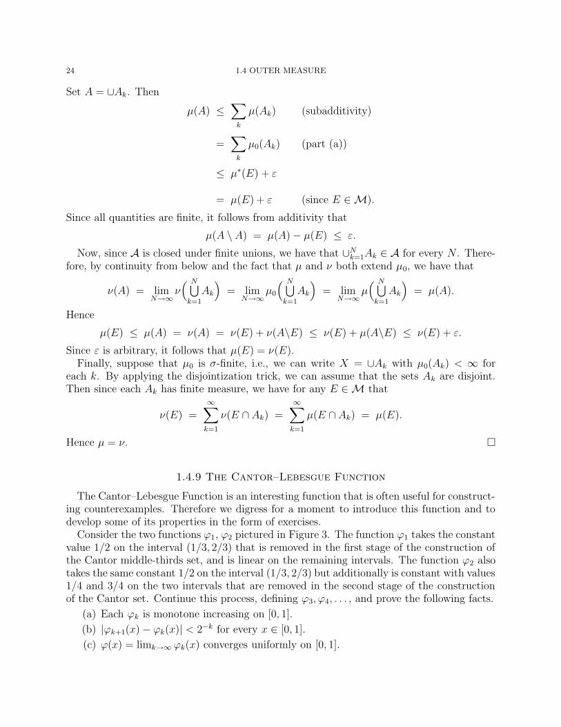
Consider the two functions ϕ1, ϕ2 pictured in Figure 3. The function ϕ1 takes the constantvalue 1/2 on the interval (1/3, 2/3) that is removed in the first stage of the construction ofthe Cantor middle-thirds set, and is linear on the remaining intervals. The function ϕ2 alsotakes the same constant 1/2 on the interval (1/3, 2/3) but additionally is constant with values1/4 and 3/4 on the two intervals that are removed in the second stage of the constructionof the Cantor set. Continue this process, defining ϕ3, ϕ4, . . . , and prove the following facts.

(a) Each ϕk is monotone increasing on [0, 1].

(b) |ϕk+1(x)− ϕk(x)| < 2−k for every x ∈ [0, 1].

(c) ϕ(x) = limk→∞ ϕk(x) converges uniformly on [0, 1].


The function ϕ constructed in this manner is called the Cantor–Lebesgue function or, morepicturesquely, the Devil’s staircase.

0.25 0.5 0.75 1

0.25

0.5

0.75

1

0.25 0.5 0.75 1

0.25

0.5

0.75

1

Figure 3. First stages in the construction of the Cantor–Lebesgue function.

Prove the following facts about ϕ.

(d) ϕ is continuous and monotone increasing on [0, 1], but ϕ is not uniformly continuous.

(e) ϕ is differentiable for a.e. x ∈ [0, 1], and ϕ′(x) = 0 a.e.

Although we have not yet defined the integral of a function like ϕ′ that is only definedalmost everywhere, we will later see after we develop the Lebesgue integral that sets of mea-sure zero “don’t matter” when dealing with integrals. As a consequence, the FundamentalTheorem of Calculus does not apply to ϕ:

ϕ(1)− ϕ(0) 6=

∫ 1

0

ϕ′(x) dx.

If we extend ϕ to R by reflecting it about the point x = 1, and then extend by zerooutside of [0, 2], we obtain the continuous function ϕ pictured in Figure 4. It is interestingthat it can be shown that ϕ is an example of a refinable function, as it satisfies the followingrefinement equation:

ϕ(x) =1

2ϕ(3x) +

1

2ϕ(3x− 1) + ϕ(3x− 2) +

1

2ϕ(3x− 3) +

1

2ϕ(3x− 4). (7)

Thus ϕ equals a finite linear combination of compressed and translated copies of itself, and soexhibits a type of self-similarity. Refinable functions are widely studied and play importantroles in wavelet theory and in subdivision schemes in computer-aided graphics.


1 2

1

Figure 4. The reflected Devil’s staircase (Cantor–Lebesgue function).

The fact that ϕ is refinable yields easy recursive algorithms for plotting ϕ to any desiredlevel of accuracy. For example, since we know the values of ϕ(k) for k integer, we cancompute the values ϕ(k/3) for k ∈ Z by considering x = k/3 in equation (7). Iterating this,we can obtain the values ϕ(k/3j) for any k ∈ Z, j ∈ N. Exercise: Plot the Cantor–Lebesguefunction.

The Cantor–Lebesgue function is the prototypical example of a singular function.

Definition 43 (Singular Function). A function f : [a, b] → C or f : R → C is singular if fis differentiable at almost every point in its domain and f ′ = 0 a.e.

1.4.10 A Nonmeasurable Set

We will give another proof of the existence of subsets of R that are not Lebesgue measur-able. To do this, we need the following theorem.

Theorem 44. If E ⊂ R is Lebesgue measurable and |E| > 0, then

E − E = {x− y : x, y ∈ E}

contains an interval around 0.

Proof. Given 0 < ε < 0, we can find an open U ⊇ E such that |U | ≤ (1 + ε) |E|. Since U isan open subset of R we can write it as a disjoint union of at most countably many intervals,say

U =⋃

k

(ak, bk).

Set Ek = E ∩ (ak, bk). Each Ek is measurable, and E is the disjoint union of the Ek.Therefore, we have

|U | =∑

k

(bk − ak) and |E| =∑

k

|Ek|.

Since |U | ≤ (1 + ε) |E|, we must have

bk − ak ≤ (1 + ε) |Ek|


for at least one k.1 Fix d with

0 < |d| <(1− ε) (bk − ak)

1 + ε.

We have that Ek ∪ (Ek + d) ⊆ (ak, bk + d) if d ≥ 0, and Ek ∪ (Ek + d) ⊆ (ak − d, bk) if d ≤ 0,In any case,

|Ek ∪ (Ek + d)| ≤ bk − ak + |d|.

If Ek and Ek + d were disjoint, then this would imply that

bk − ak + |d| ≥ |Ek ∩ (Ek + d)| = |Ek|+ |Ek + d| ≥2(bk − ak)

1 + ε.

Regarranging, we find that

|d| ≥(1− ε) (bk − ak)

1 + ε,

which is a contradiction. Therefore Ek∩(Ek +d) 6= ∅ for all |d| small enough. Hence Ek−Ek

contains an interval, and therefore E − E does as well. �

Exercise 45. Define an equivalence relation ∼ on R by

x ∼ y ⇐⇒ x− y ∈ Q.

By the Axiom of Choice, there exists a set N that contains exactly one element of eachequivalence class for ∼. Show that N − N contains no intervals and that |N |e > 0, andconclude that N is not Lebesgue measurable.

Exercises

Here are some practice exercises on Lebesgue measure on Rd, mostly taken from the textby Wheeden and Zygmund. Be sure to also work the exercises on abstract measure theoryfrom Folland’s text.

1. Construct a subset of [0, 1] in the same manner as the Cantor set, except that at thekth stage, each interval removed has length δ3−k, where 0 < δ < 1 is fixed. Showthat the resulting set has measure 1− δ and contains no intervals.

2. If {Ek}∞k=1 is a sequence of sets with

∑

|Ek|e <∞, show that lim sup Ek (and so alsolim inf Ek) has measure zero.

3. Show that if E1 is a measurable subset of Rm and E2 is a measurable subset of Rn,then E1 × E2 is a measurable subset of Rm+n, and

|E1 × E2| = |E1| |E2|.

Note: Interpret 0 · ∞ as 0.Hint: Use an equivalent characterization of measurability.Remark: This is an important fact that we will need to use later.

1That is, for at least one k, on at least one side.


3. Recall from Theorem 9 that if E ⊆ Rd, then its exterior measure satisfies

|E|e = inf{

|U |e : U open, U ⊇ E}

.

Define the inner Lebesgue measure of E to be

|E|i = sup{

|F | : F closed, F ⊆ E}

.

Prove that |E|i ≤ |E|e. Show that if |E|e < ∞, then E is Lebesgue measurable ifand only if |E|e = |E|i. Give an example that shows that this equivalence can fail if|E|e =∞.

4. Show that if E ⊆ Rd is measurable and A ⊆ E, then |E| = |A|i + |E\A|e.

5. Give an example of a continuous function f : R → R and a measurable set E ⊆ Rsuch that f(E) is not measurable.

Hint: Consider the Cantor–Lebesgue function and the preimage of an appropriatenonmeasurable subset of its range.

6. Show that there exist disjoint E1, E2, . . . such that∣

∣

∣

∞⋃

k=1

Ek

∣

∣

∣

e<

∞∑

k=1

|Ek|e,

with strict inequality.Hint: Let E be a nonmeasurable subset of [0, 1] whose rational translates are

disjoint. Consider the translates of E by all rational r ∈ (0, 1), and use the fact thatexterior Lebesgue measure is translation-invariant.

7. Show that there exist E1 ⊇ E2 ⊇ . . . such that |Ek|e <∞ for every k and∣

∣

∣

∞⋂

k=1

Ek

∣

∣

∣

e< lim

k→∞|Ek|e,

with strict inequality.

8. Show that if Z ⊆ R has measure zero, then so does {x2 : x ∈ Z}.

real analysis lecture notes: 1.4 outer measure...

Documents