Video coveringthis content is

available online.

The following is a review of the Quantitative Methods (2) designed to address the learning outcomestatements set forth by CFA Institute. Cross-Reference to CFA Institute Assigned Reading #12.

READING 12: HYPOTHESIS TESTINGStudy Session 3

EXAM FOCUSThis review addresses common hypothesis testing procedures. These procedures areused to conduct tests of population means, population variances, differences in means,differences in variances, and mean differences. Specific tests reviewed include the z-test, t-test, chi-square test, and F-test. You should know when and how to apply each ofthese. A standard hypothesis testing procedure is utilized in this review. Know it! Youshould be able to perform a hypothesis test on the value of the mean without beinggiven any formulas. Confidence intervals, levels of significance, the power of a test, andtypes of hypothesis testing errors are also discussed. Don’t worry about memorizing themessy formulas on testing for the equalities and differences in means and variances atthe end of this review, but be able to interpret these statistics.

MODULE 12.1: HYPOTHESIS TESTS ANDTYPES OF ERRORSHypothesis testing is the statistical assessment of a statement or idearegarding a population. For instance, a statement could be as follows:“The mean return for the U.S. equity market is greater than zero.” Given the relevantreturns data, hypothesis testing procedures can be employed to test the validity of thisstatement at a given significance level.

LOS 12.a: Define a hypothesis, describe the steps of hypothesis testing, anddescribe and interpret the choice of the null and alternative hypotheses.

CFA® Program Curriculum, Volume 1, page 621A hypothesis is a statement about the value of a population parameter developed for thepurpose of testing a theory or belief. Hypotheses are stated in terms of the populationparameter to be tested, like the population mean, µ. For example, a researcher may beinterested in the mean daily return on stock options. Hence, the hypothesis may be thatthe mean daily return on a portfolio of stock options is positive.Hypothesis testing procedures, based on sample statistics and probability theory, areused to determine whether a hypothesis is a reasonable statement and should not berejected or if it is an unreasonable statement and should be rejected. The process ofhypothesis testing consists of a series of steps shown in Figure 12.1.

Figure 12.1: Hypothesis Testing Procedure*

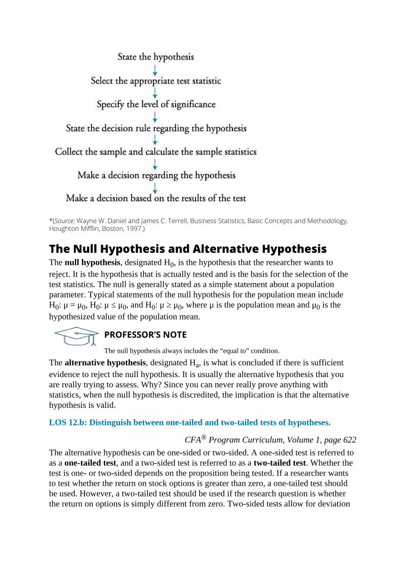
*(Source: Wayne W. Daniel and James C. Terrell, Business Statistics, Basic Concepts and Methodology,Houghton Mifflin, Boston, 1997.)

The Null Hypothesis and Alternative HypothesisThe null hypothesis, designated H0, is the hypothesis that the researcher wants toreject. It is the hypothesis that is actually tested and is the basis for the selection of thetest statistics. The null is generally stated as a simple statement about a populationparameter. Typical statements of the null hypothesis for the population mean includeH0: μ = μ0, H0: μ ≤ μ0, and H0: μ ≥ μ0, where μ is the population mean and μ0 is thehypothesized value of the population mean.

PROFESSOR’S NOTE

The null hypothesis always includes the “equal to” condition.

The alternative hypothesis, designated Ha, is what is concluded if there is sufficientevidence to reject the null hypothesis. It is usually the alternative hypothesis that youare really trying to assess. Why? Since you can never really prove anything withstatistics, when the null hypothesis is discredited, the implication is that the alternativehypothesis is valid.

LOS 12.b: Distinguish between one-tailed and two-tailed tests of hypotheses.

CFA® Program Curriculum, Volume 1, page 622The alternative hypothesis can be one-sided or two-sided. A one-sided test is referred toas a one-tailed test, and a two-sided test is referred to as a two-tailed test. Whether thetest is one- or two-sided depends on the proposition being tested. If a researcher wantsto test whether the return on stock options is greater than zero, a one-tailed test shouldbe used. However, a two-tailed test should be used if the research question is whetherthe return on options is simply different from zero. Two-sided tests allow for deviation

on both sides of the hypothesized value (zero). In practice, most hypothesis tests areconstructed as two-tailed tests.A two-tailed test for the population mean may be structured as:

H0: μ = μ0 versus Ha: μ ≠ μ0

Since the alternative hypothesis allows for values above and below the hypothesizedparameter, a two-tailed test uses two critical values (or rejection points).The general decision rule for a two-tailed test is:

Reject H0 if: test statistic > upper critical value or test statistic < lower critical value

Let’s look at the development of the decision rule for a two-tailed test using a z-distributed test statistic (a z-test) at a 5% level of significance, α = 0.05.

At α = 0.05, the computed test statistic is compared with the critical z-values of±1.96. The values of ±1.96 correspond to ±zα/2 = ±z0.025, which is the range of z-values within which 95% of the probability lies. These values are obtained fromthe cumulative probability table for the standard normal distribution (z-table),which is included at the back of this book.If the computed test statistic falls outside the range of critical z-values (i.e., teststatistic > 1.96, or test statistic < –1.96), we reject the null and conclude that thesample statistic is sufficiently different from the hypothesized value.If the computed test statistic falls within the range ±1.96, we conclude that thesample statistic is not sufficiently different from the hypothesized value (μ = μ0 inthis case), and we fail to reject the null hypothesis.

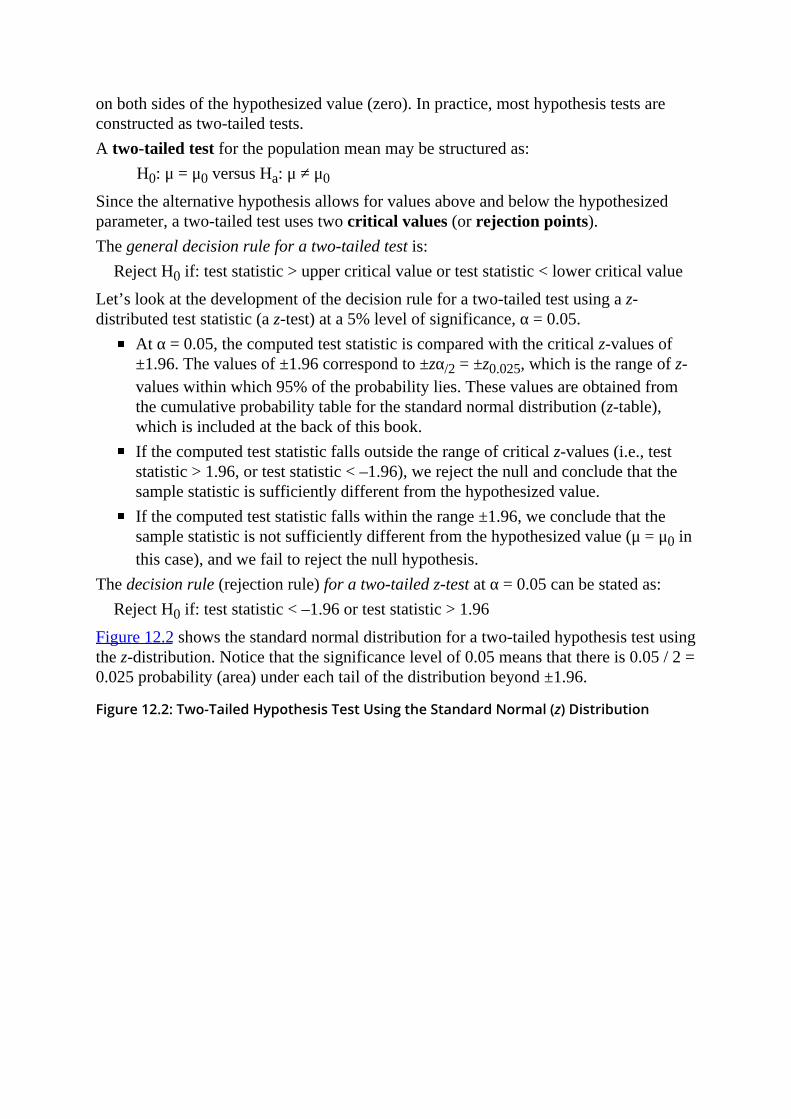
The decision rule (rejection rule) for a two-tailed z-test at α = 0.05 can be stated as:Reject H0 if: test statistic < –1.96 or test statistic > 1.96

Figure 12.2 shows the standard normal distribution for a two-tailed hypothesis test usingthe z-distribution. Notice that the significance level of 0.05 means that there is 0.05 / 2 =0.025 probability (area) under each tail of the distribution beyond ±1.96.

Figure 12.2: Two-Tailed Hypothesis Test Using the Standard Normal (z) Distribution

For a one-tailed hypothesis test of the population mean, the null and alternativehypotheses are either:

Upper tail: H0: μ ≤ μ0 versus Ha: μ > μ0, orLower tail: H0: μ ≥ μ0 versus Ha: μ < μ0

The appropriate set of hypotheses depends on whether we believe the population mean,μ, to be greater than (upper tail) or less than (lower tail) the hypothesized value, μ0.Using a z-test at the 5% level of significance, the computed test statistic is comparedwith the critical values of 1.645 for the upper tail tests (i.e., Ha: μ > μ0) or –1.645 forlower tail tests (i.e., Ha: μ < μ0). These critical values are obtained from a z-table, where–z0.05 = –1.645 corresponds to a cumulative probability equal to 5%, and the z0.05 =1.645 corresponds to a cumulative probability of 95% (1 − 0.05).Let’s use the upper tail test structure where H0: µ ≤ µ0 and Ha: µ > µ0.

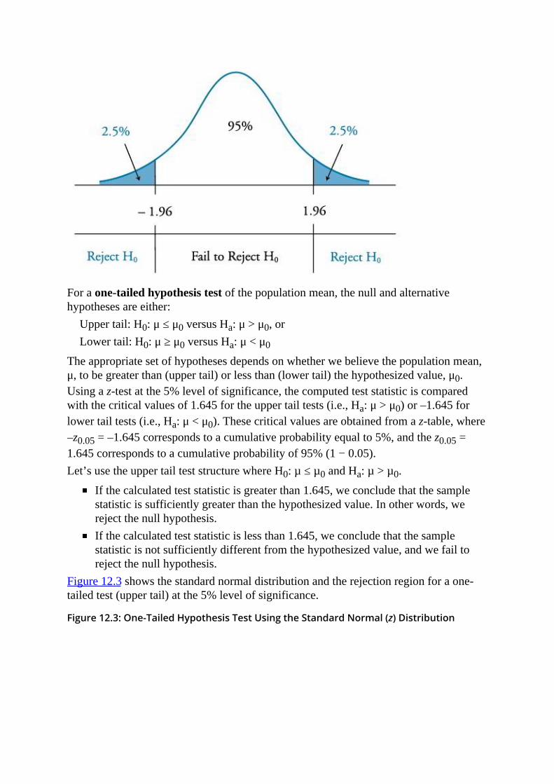
If the calculated test statistic is greater than 1.645, we conclude that the samplestatistic is sufficiently greater than the hypothesized value. In other words, wereject the null hypothesis.If the calculated test statistic is less than 1.645, we conclude that the samplestatistic is not sufficiently different from the hypothesized value, and we fail toreject the null hypothesis.

Figure 12.3 shows the standard normal distribution and the rejection region for a one-tailed test (upper tail) at the 5% level of significance.

Figure 12.3: One-Tailed Hypothesis Test Using the Standard Normal (z) Distribution

The Choice of the Null and Alternative HypothesesThe most common null hypothesis will be an “equal to” hypothesis. Combined with a“not equal to” alternative, this will require a two-tailed test. The alternative is often thehoped-for hypothesis. The null will include the “equal to” sign and the alternative willinclude the “not equal to” sign. When the null is that a coefficient is equal to zero, wehope to reject it and show the significance of the relationship.When the null is less than or equal to, the (mutually exclusive) alternative is framed asgreater than, and a one-tail test is appropriate. If we are trying to demonstrate that areturn is greater than the risk-free rate, this would be the correct formulation. We willhave set up the null and alternative hypothesis so that rejection of the null will lead toacceptance of the alternative, our goal in performing the test. As with a two-tailed test,the null for a one-tailed test will include the “equal to” sign (i.e., either “greater than orequal to” or “less than or equal to”). The alternative will include the opposite sign to thenull—either “less than” or “greater than.”

LOS 12.c: Explain a test statistic, Type I and Type II errors, a significance level,and how significance levels are used in hypothesis testing.

CFA® Program Curriculum, Volume 1, page 623Hypothesis testing involves two statistics: the test statistic calculated from the sampledata and the critical value of the test statistic. The value of the computed test statisticrelative to the critical value is a key step in assessing the validity of a hypothesis.A test statistic is calculated by comparing the point estimate of the population parameterwith the hypothesized value of the parameter (i.e., the value specified in the nullhypothesis). With reference to our option return example, this means we are concernedwith the difference between the mean return of the sample (i.e., x = 0.001) and thehypothesized mean return (i.e., µ0 = 0). As indicated in the following expression, thetest statistic is the difference between the sample statistic and the hypothesized value,scaled by the standard error of the sample statistic.

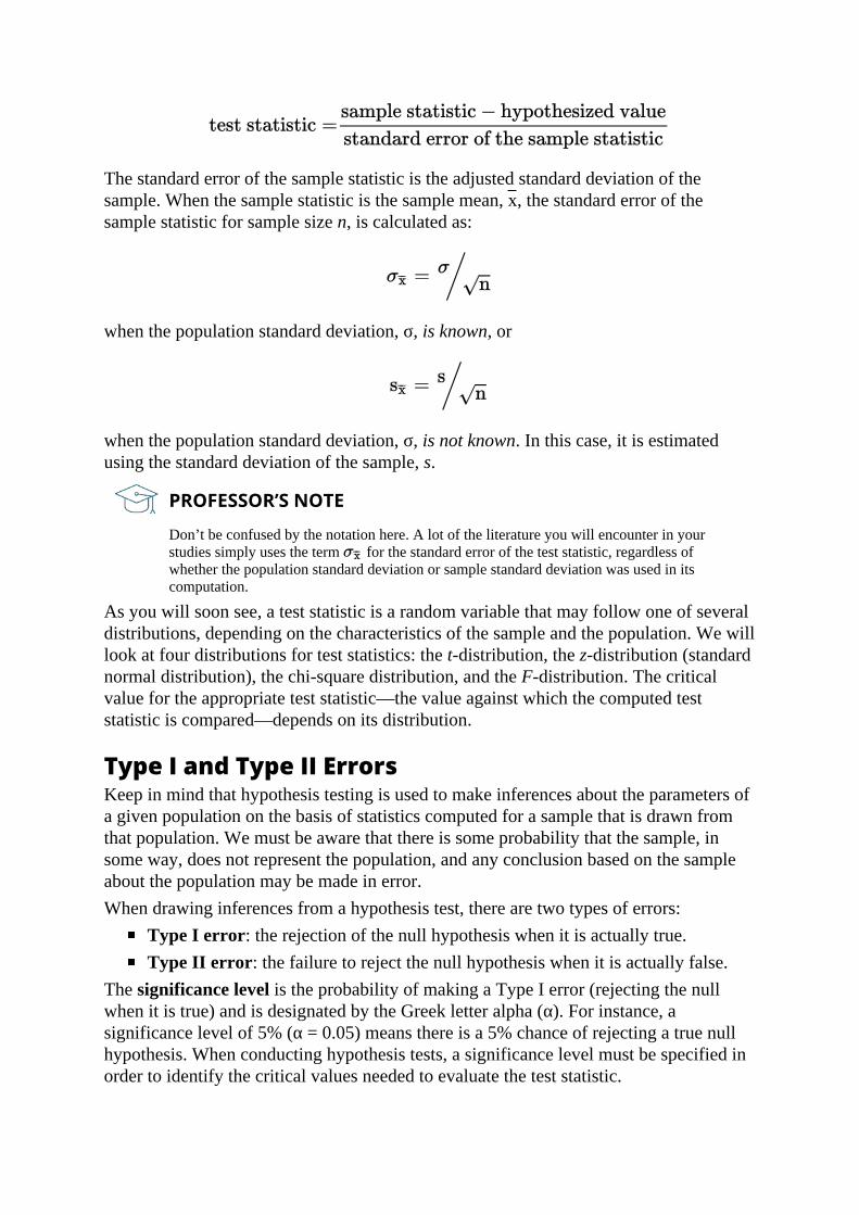
The standard error of the sample statistic is the adjusted standard deviation of thesample. When the sample statistic is the sample mean, x, the standard error of thesample statistic for sample size n, is calculated as:

when the population standard deviation, σ, is known, or

when the population standard deviation, σ, is not known. In this case, it is estimatedusing the standard deviation of the sample, s.

PROFESSOR’S NOTE

Don’t be confused by the notation here. A lot of the literature you will encounter in yourstudies simply uses the term for the standard error of the test statistic, regardless ofwhether the population standard deviation or sample standard deviation was used in itscomputation.

As you will soon see, a test statistic is a random variable that may follow one of severaldistributions, depending on the characteristics of the sample and the population. We willlook at four distributions for test statistics: the t-distribution, the z-distribution (standardnormal distribution), the chi-square distribution, and the F-distribution. The criticalvalue for the appropriate test statistic—the value against which the computed teststatistic is compared—depends on its distribution.

Type I and Type II ErrorsKeep in mind that hypothesis testing is used to make inferences about the parameters ofa given population on the basis of statistics computed for a sample that is drawn fromthat population. We must be aware that there is some probability that the sample, insome way, does not represent the population, and any conclusion based on the sampleabout the population may be made in error.When drawing inferences from a hypothesis test, there are two types of errors:

Type I error: the rejection of the null hypothesis when it is actually true.Type II error: the failure to reject the null hypothesis when it is actually false.

The significance level is the probability of making a Type I error (rejecting the nullwhen it is true) and is designated by the Greek letter alpha (α). For instance, asignificance level of 5% (α = 0.05) means there is a 5% chance of rejecting a true nullhypothesis. When conducting hypothesis tests, a significance level must be specified inorder to identify the critical values needed to evaluate the test statistic.

LOS 12.d: Explain a decision rule, the power of a test, and the relation betweenconfidence intervals and hypothesis tests.

CFA® Program Curriculum, Volume 1, page 625The decision for a hypothesis test is to either reject the null hypothesis or fail to rejectthe null hypothesis. Note that it is statistically incorrect to say “accept” the nullhypothesis; it can only be supported or rejected. The decision rule for rejecting orfailing to reject the null hypothesis is based on the distribution of the test statistic. Forexample, if the test statistic follows a normal distribution, the decision rule is based oncritical values determined from the standard normal distribution (z-distribution).Regardless of the appropriate distribution, it must be determined if a one-tailed or two-tailed hypothesis test is appropriate before a decision rule (rejection rule) can bedetermined.A decision rule is specific and quantitative. Once we have determined whether a one- ortwo-tailed test is appropriate, the significance level we require, and the distribution ofthe test statistic, we can calculate the exact critical value for the test statistic. Then wehave a decision rule of the following form: if the test statistic is (greater, less than) thevalue X, reject the null.

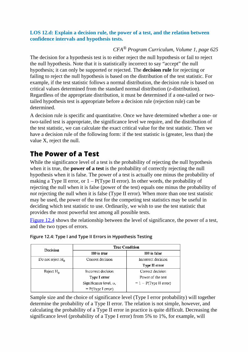
The Power of a TestWhile the significance level of a test is the probability of rejecting the null hypothesiswhen it is true, the power of a test is the probability of correctly rejecting the nullhypothesis when it is false. The power of a test is actually one minus the probability ofmaking a Type II error, or 1 – P(Type II error). In other words, the probability ofrejecting the null when it is false (power of the test) equals one minus the probability ofnot rejecting the null when it is false (Type II error). When more than one test statisticmay be used, the power of the test for the competing test statistics may be useful indeciding which test statistic to use. Ordinarily, we wish to use the test statistic thatprovides the most powerful test among all possible tests.Figure 12.4 shows the relationship between the level of significance, the power of a test,and the two types of errors.

Figure 12.4: Type I and Type II Errors in Hypothesis Testing

Sample size and the choice of significance level (Type I error probability) will togetherdetermine the probability of a Type II error. The relation is not simple, however, andcalculating the probability of a Type II error in practice is quite difficult. Decreasing thesignificance level (probability of a Type I error) from 5% to 1%, for example, will

increase the probability of failing to reject a false null (Type II error) and thereforereduce the power of the test. Conversely, for a given sample size, we can increase thepower of a test only with the cost that the probability of rejecting a true null (Type Ierror) increases. For a given significance level, we can decrease the probability of aType II error and increase the power of a test, only by increasing the sample size.

The Relation Between Confidence Intervals andHypothesis TestsA confidence interval is a range of values within which the researcher believes the truepopulation parameter may lie.A confidence interval is determined as:

The interpretation of a confidence interval is that for a level of confidence of 95%, forexample, there is a 95% probability that the true population parameter is contained inthe interval.From the previous expression, we see that a confidence interval and a hypothesis testare linked by the critical value. For example, a 95% confidence interval uses a criticalvalue associated with a given distribution at the 5% level of significance. Similarly, ahypothesis test would compare a test statistic to a critical value at the 5% level ofsignificance. To see this relationship more clearly, the expression for the confidenceinterval can be manipulated and restated as:

–critical value ≤ test statistic ≤ +critical valueThis is the range within which we fail to reject the null for a two-tailed hypothesis testat a given level of significance.

EXAMPLE: Confidence intervals and two-tailed hypothesis tests

A researcher has gathered data on the daily returns on a portfolio of call options over a recent 250-dayperiod. The mean daily return has been 0.1%, and the sample standard deviation of daily portfolioreturns is 0.25%. The researcher believes that the mean daily portfolio return is not equal to zero.

1. Construct a 95% confidence interval for the population mean daily return over the 250-daysample period.

2. Construct a hypothesis test of the researcher’s belief.Answer:1. Given a sample size of 250 with a standard deviation of 0.25%, the standard error can be computedas .

At the 5% level of significance, the critical z-values for the confidence interval are z0.025 = 1.96 and–z0.025 = –1.96. Thus, given a sample mean equal to 0.1%, the 95% confidence interval for thepopulation mean is:

Video covering

0.1 − 1.96(0.0158) ≤ µ ≤ 0.1 + 1.96(0.0158), or0.069% ≤ µ ≤ 0.131%

2. First we need to specify the null and alternative hypotheses. The null hypothesis is the one theresearcher expects to reject.

H0: μ0 = 0 versus Ha: μ0 ≠ 0Since the null hypothesis is an equality, this is a two-tailed test. At a 5% level of significance, thecritical z-values for a two-tailed test are ±1.96, so the decision rule can be stated as:

Reject H0 if test statistic < –1.96 or test statistic > +1.96Using the standard error of the sample mean we calculated above, our test statistic is:

Since 6.33 > 1.96, we reject the null hypothesis that the mean daily option return is equal to zero.Notice the similarity of this analysis with our confidence interval. We rejected the hypothesis µ = 0because the sample mean of 0.1% is more than 1.96 standard errors from zero. Based on the 95%confidence interval, we reject µ = 0 because zero is more than 1.96 standard errors from the samplemean of 0.1%.

MODULE QUIZ 12.1

To best evaluate your performance, enter your quiz answers online.

1. To test whether the mean of a population is greater than 20, the appropriate nullhypothesis is that the population mean is:

A. less than 20.B. greater than 20.C. less than or equal to 20.

2. Which of the following statements about hypothesis testing is most accurate?A. A Type II error is rejecting the null when it is actually true.B. The significance level equals one minus the probability of a Type I error.C. A two-tailed test with a significance level of 5% has z-critical values of ±1.96.

3. For a hypothesis test with a probability of a Type II error of 60% and a probabilityof a Type I error of 5%, which of the following statements is most accurate?

A. The power of the test is 40%, and there is a 5% probability that the teststatistic will exceed the critical value(s).

B. There is a 95% probability that the test statistic will be between the criticalvalues if this is a two-tailed test.

C. There is a 5% probability that the null hypothesis will be rejected whenactually true, and the probability of rejecting the null when it is false is 40%.

4. If the significance level of a test is 0.05 and the probability of a Type II error is0.15, what is the power of the test?

A. 0.850.B. 0.950.C. 0.975.

MODULE 12.2: TESTS OF MEANS AND P-VALUES

Video coveringthis content is

available online.

MODULE 12.2: TESTS OF MEANS AND P-VALUESLOS 12.e: Distinguish between a statistical result and aneconomically meaningful result.

CFA® Program Curriculum, Volume 1, page 629Statistical significance does not necessarily imply economic significance. Forexample, we may have tested a null hypothesis that a strategy of going long all thestocks that satisfy some criteria and shorting all the stocks that do not satisfy the criteriaresulted in returns that were less than or equal to zero over a 20-year period. Assume wehave rejected the null in favor of the alternative hypothesis that the returns to thestrategy are greater than zero (positive). This does not necessarily mean that investing inthat strategy will result in economically meaningful positive returns. Several factorsmust be considered.One important consideration is transactions costs. Once we consider the costs of buyingand selling the securities, we may find that the mean positive returns to the strategy arenot enough to generate positive returns. Taxes are another factor that may make aseemingly attractive strategy a poor one in practice. A third reason that statisticallysignificant results may not be economically significant is risk. In the above strategy, wehave additional risk from short sales (they may have to be closed out earlier than in thetest strategy). Since the statistically significant results were for a period of 20 years, itmay be the case that there is significant variation from year to year in the returns fromthe strategy, even though the mean strategy return is greater than zero. This variation inreturns from period to period is an additional risk to the strategy that is not accountedfor in our test of statistical significance.Any of these factors could make committing funds to a strategy unattractive, eventhough the statistical evidence of positive returns is highly significant. By the nature ofstatistical tests, a very large sample size can result in highly (statistically) significantresults that are quite small in absolute terms.

LOS 12.f: Explain and interpret the p-value as it relates to hypothesis testing.

CFA® Program Curriculum, Volume 1, page 629The p-value is the probability of obtaining a test statistic that would lead to a rejectionof the null hypothesis, assuming the null hypothesis is true. It is the smallest level ofsignificance for which the null hypothesis can be rejected. For one-tailed tests, the p-value is the probability that lies above the computed test statistic for upper tail tests orbelow the computed test statistic for lower tail tests. For two-tailed tests, the p-value isthe probability that lies above the positive value of the computed test statistic plus theprobability that lies below the negative value of the computed test statistic.Consider a two-tailed hypothesis test about the mean value of a random variable at the95% significance level where the test statistic is 2.3, greater than the upper critical valueof 1.96. If we consult the Z-table, we find the probability of getting a value greater than2.3 is (1 − 0.9893) = 1.07%. Since it’s a two-tailed test, our p-value is 2 × 1.07 = 2.14%,as illustrated in Figure 12.5. At a 3%, 4%, or 5% significance level, we would reject the

null hypothesis, but at a 2% or 1% significance level we would not. Many researchersreport p-values without selecting a significance level and allow the reader to judge howstrong the evidence for rejection is.

Figure 12.5: Two-Tailed Hypothesis Test with p-value = 2.14%

LOS 12.g: Identify the appropriate test statistic and interpret the results for ahypothesis test concerning the population mean of both large and small sampleswhen the population is normally or approximately normally distributed and thevariance is 1) known or 2) unknown.

CFA® Program Curriculum, Volume 1, page 630When hypothesis testing, the choice between using a critical value based on the t-distribution or the z-distribution depends on sample size, the distribution of thepopulation, and whether or not the variance of the population is known.

The t-TestThe t-test is a widely used hypothesis test that employs a test statistic that is distributedaccording to a t-distribution. Following are the rules for when it is appropriate to use thet-test for hypothesis tests of the population mean.Use the t-test if the population variance is unknown and either of the followingconditions exist:

The sample is large (n ≥ 30).The sample is small (less than 30), but the distribution of the population is normalor approximately normal.

If the sample is small and the distribution is nonnormal, we have no reliable statisticaltest.The computed value for the test statistic based on the t-distribution is referred to as thet-statistic. For hypothesis tests of a population mean, a t-statistic with n – 1 degrees offreedom is computed as:

where:x = sample meanμ0 = hypothesized population mean (i.e., the null)s = standard deviation of the samplen = sample size

PROFESSOR’S NOTE

This computation is not new. It is the same test statistic computation that we have beenperforming all along. Note the use of the sample standard deviation, s, in the standard errorterm in the denominator.

To conduct a t-test, the t-statistic is compared to a critical t-value at the desired level ofsignificance with the appropriate degrees of freedom.In the real world, the underlying variance of the population is rarely known, so the t-testenjoys widespread application.

The z-TestThe z-test is the appropriate hypothesis test of the population mean when the populationis normally distributed with known variance. The computed test statistic used with thez-test is referred to as the z-statistic. The z-statistic for a hypothesis test for a populationmean is computed as follows:

where:x = sample meanμ0 = hypothesized population meanσ = standard deviation of the populationn = sample size

To test a hypothesis, the z-statistic is compared to the critical z-value corresponding tothe significance of the test. Critical z-values for the most common levels of significanceare displayed in Figure 12.6. You should have these memorized by now.

Figure 12.6: Critical z-Values

When the sample size is large and the population variance is unknown, the z-statistic is:

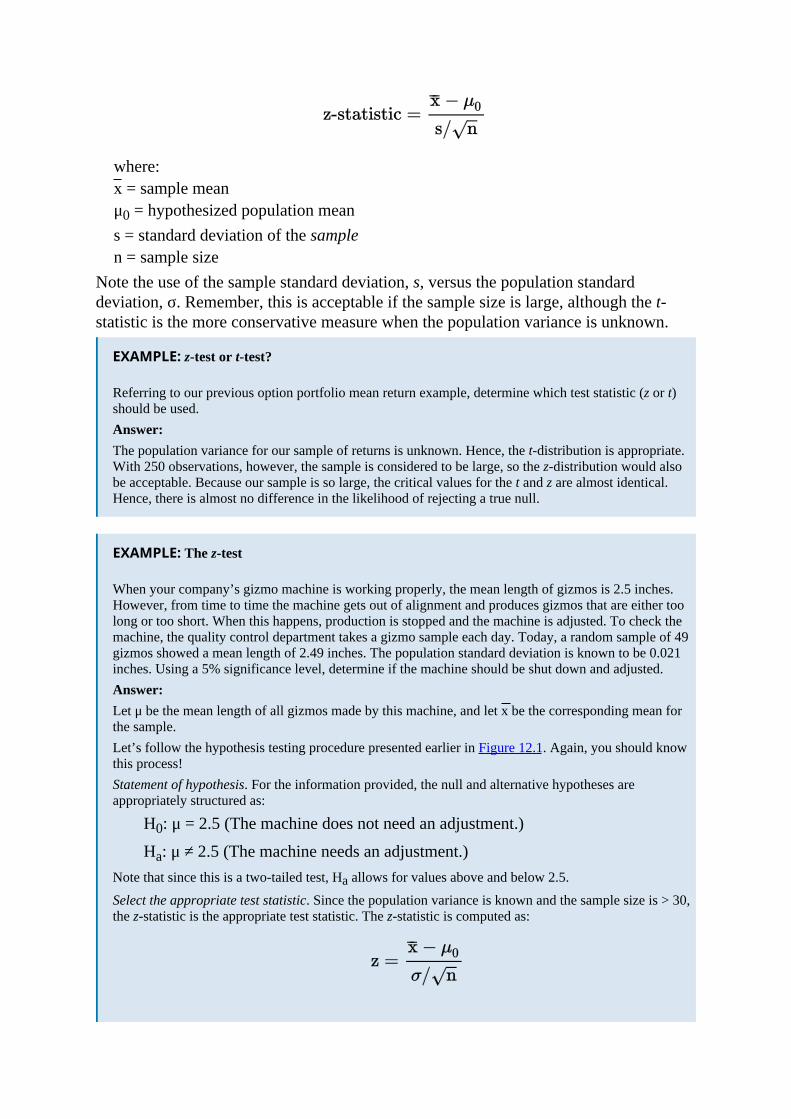
where:x = sample meanμ0 = hypothesized population means = standard deviation of the samplen = sample size

Note the use of the sample standard deviation, s, versus the population standarddeviation, σ. Remember, this is acceptable if the sample size is large, although the t-statistic is the more conservative measure when the population variance is unknown.

EXAMPLE: z-test or t-test?

Referring to our previous option portfolio mean return example, determine which test statistic (z or t)should be used.Answer:The population variance for our sample of returns is unknown. Hence, the t-distribution is appropriate.With 250 observations, however, the sample is considered to be large, so the z-distribution would alsobe acceptable. Because our sample is so large, the critical values for the t and z are almost identical.Hence, there is almost no difference in the likelihood of rejecting a true null.

EXAMPLE: The z-test

When your company’s gizmo machine is working properly, the mean length of gizmos is 2.5 inches.However, from time to time the machine gets out of alignment and produces gizmos that are either toolong or too short. When this happens, production is stopped and the machine is adjusted. To check themachine, the quality control department takes a gizmo sample each day. Today, a random sample of 49gizmos showed a mean length of 2.49 inches. The population standard deviation is known to be 0.021inches. Using a 5% significance level, determine if the machine should be shut down and adjusted.Answer:Let μ be the mean length of all gizmos made by this machine, and let x be the corresponding mean forthe sample.Let’s follow the hypothesis testing procedure presented earlier in Figure 12.1. Again, you should knowthis process!Statement of hypothesis. For the information provided, the null and alternative hypotheses areappropriately structured as:

H0: μ = 2.5 (The machine does not need an adjustment.)

Ha: μ ≠ 2.5 (The machine needs an adjustment.)Note that since this is a two-tailed test, Ha allows for values above and below 2.5.

Select the appropriate test statistic. Since the population variance is known and the sample size is > 30,the z-statistic is the appropriate test statistic. The z-statistic is computed as:

Specify the level of significance. The level of significance is given at 5%, implying that we are willingto accept a 5% probability of rejecting a true null hypothesis.State the decision rule regarding the hypothesis. The ≠ sign in the alternative hypothesis indicates thatthe test is two-tailed with two rejection regions, one in each tail of the standard normal distributioncurve. Because the total area of both rejection regions combined is 0.05 (the significance level), thearea of the rejection region in each tail is 0.025. You should know that the critical z-values for ±z0.025are ±1.96. This means that the null hypothesis should not be rejected if the computed z-statistic liesbetween –1.96 and +1.96 and should be rejected if it lies outside of these critical values. The decisionrule can be stated as:

Reject H0 if –z0.025 > z-statistic > z0.025, or equivalently,

Reject H0 if: –1.96 > z-statistic > + 1.96Collect the sample and calculate the test statistic. The value of x from the sample is 2.49. Since σ isgiven as 0.021, we calculate the z-statistic using σ as follows:

Make a decision regarding the hypothesis. The calculated value of the z-statistic is –3.33. Since thisvalue is less than the critical value, –z0.025 = –1.96, it falls in the rejection region in the left tail of thez-distribution. Hence, there is sufficient evidence to reject H0.

Make a decision based on the results of the test. Based on the sample information and the results of thetest, it is concluded that the machine is out of adjustment and should be shut down for repair.

EXAMPLE: One-tailed test

Using the data from the previous example and a 5% significance level, test the hypothesis that themean length of gizmos is less than 2.5 inches.Answer:In this case, we use a one-tailed test with the following structure:

H0: μ ≥ 2.5 versus Ha: μ < 2.5The appropriate decision rule for this one-tailed test at a significance level of 5% is:

Reject H0 if test statistic < –1.645The test statistic is computed in the same way, regardless of whether we are using a one-tailed or atwo-tailed test. From the previous example, we know that the test statistic for the gizmo sample is –3.33. Because –3.33 < –1.645, we can reject the null hypothesis and conclude that the mean length isstatistically less than 2.5 at a 5% level of significance.

MODULE QUIZ 12.2

To best evaluate your performance, enter your quiz answers online.

1. Using historical data, a hedge fund manager designs a test of whether abnormalreturns are positive on average. The test results in a p-value of 3%. The managercan most appropriately:

A. reject the hypothesis that abnormal returns are less than or equal to zero,using a 1% significance level.

B. reject the hypothesis that abnormal returns are less than or equal to zero,using a 5% significance level.

Video coveringthis content is

available online.

C. conclude that the strategy produces positive abnormal returns on average,using a 5% significance level.

2. An analyst wants to test a hypothesis concerning the population mean of monthlyreturns for a composite that has existed for 24 months. The analyst mayappropriately use:

A. a t-test but not a z-test if returns for the composite are normallydistributed.

B. either a t-test or a z-test if returns for the composite are normallydistributed.

C. a t-test but not a z-test, regardless of the distribution of returns for thecomposite.

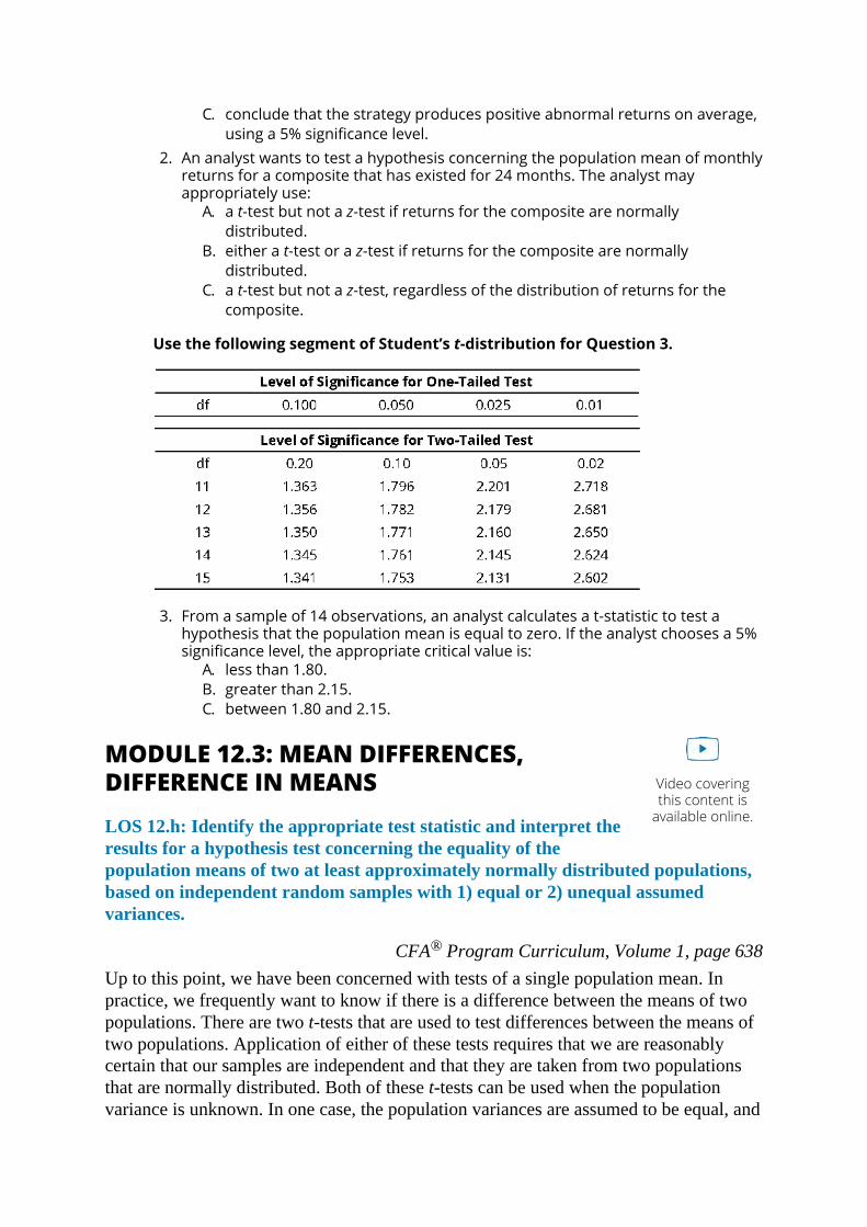
Use the following segment of Student’s t-distribution for Question 3.

3. From a sample of 14 observations, an analyst calculates a t-statistic to test ahypothesis that the population mean is equal to zero. If the analyst chooses a 5%significance level, the appropriate critical value is:

A. less than 1.80.B. greater than 2.15.C. between 1.80 and 2.15.

MODULE 12.3: MEAN DIFFERENCES,DIFFERENCE IN MEANSLOS 12.h: Identify the appropriate test statistic and interpret theresults for a hypothesis test concerning the equality of thepopulation means of two at least approximately normally distributed populations,based on independent random samples with 1) equal or 2) unequal assumedvariances.

CFA® Program Curriculum, Volume 1, page 638Up to this point, we have been concerned with tests of a single population mean. Inpractice, we frequently want to know if there is a difference between the means of twopopulations. There are two t-tests that are used to test differences between the means oftwo populations. Application of either of these tests requires that we are reasonablycertain that our samples are independent and that they are taken from two populationsthat are normally distributed. Both of these t-tests can be used when the populationvariance is unknown. In one case, the population variances are assumed to be equal, and

the sample observations are pooled. In the other case, however, no assumption is maderegarding the equality between the two population variances, and the t-test uses anapproximated value for the degrees of freedom.

PROFESSOR’S NOTE

Please note the language of the LOS here. Candidates must “Identify the appropriate teststatistic and interpret the results of a hypothesis test….” Certainly you should know that thisis a t-test, and that we reject the hypothesis of equality when the test statistic is outside thecritical t-values. Don’t worry about memorizing the following formulas. You shouldunderstand, however, that we can pool the data to get the standard deviation of the differencein means when we assume equal variances, while both sample variances are used to get thestandard error of the difference in means when we assume the population variances are notequal.

A pooled variance is used with the t-test for testing the hypothesis that the means of twonormally distributed populations are equal, when the variances of the populations areunknown but assumed to be equal.Assuming independent samples, the t-statistic in this case is computed as:

where:

= variance of the first sample = variance of the second sample

n1 = number of observations in the first samplen2 = number of observations in the second sample

Note: The degrees of freedom, df, is (n1 + n2 − 2).

Since we assume that the variances are equal, we just add the variances of the twosample means in order to calculate the standard error in the denominator.The t-test for equality of population means when the populations are normallydistributed and have variances that are unknown and assumed to be unequal usesthe sample variances for both populations. Assuming independent samples, the t-statistic in this case is computed as follows:

where:

and where: = variance of the first sample = variance of the second sample

n1 = number of observations in the first samplen2 = number of observations in the second sample

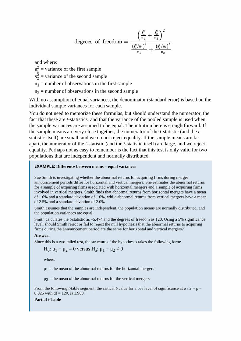
With no assumption of equal variances, the denominator (standard error) is based on theindividual sample variances for each sample.You do not need to memorize these formulas, but should understand the numerator, thefact that these are t-statistics, and that the variance of the pooled sample is used whenthe sample variances are assumed to be equal. The intuition here is straightforward. Ifthe sample means are very close together, the numerator of the t-statistic (and the t-statistic itself) are small, and we do not reject equality. If the sample means are farapart, the numerator of the t-statistic (and the t-statistic itself) are large, and we rejectequality. Perhaps not as easy to remember is the fact that this test is only valid for twopopulations that are independent and normally distributed.

EXAMPLE: Difference between means – equal variances

Sue Smith is investigating whether the abnormal returns for acquiring firms during mergerannouncement periods differ for horizontal and vertical mergers. She estimates the abnormal returnsfor a sample of acquiring firms associated with horizontal mergers and a sample of acquiring firmsinvolved in vertical mergers. Smith finds that abnormal returns from horizontal mergers have a meanof 1.0% and a standard deviation of 1.0%, while abnormal returns from vertical mergers have a meanof 2.5% and a standard deviation of 2.0%.Smith assumes that the samples are independent, the population means are normally distributed, andthe population variances are equal.Smith calculates the t-statistic as –5.474 and the degrees of freedom as 120. Using a 5% significancelevel, should Smith reject or fail to reject the null hypothesis that the abnormal returns to acquiringfirms during the announcement period are the same for horizontal and vertical mergers?Answer:Since this is a two-tailed test, the structure of the hypotheses takes the following form:

H0: μ1 − μ2 = 0 versus Ha: μ1 − μ2 ≠ 0

where:

μ1 = the mean of the abnormal returns for the horizontal mergers

μ2 = the mean of the abnormal returns for the vertical mergers

From the following t-table segment, the critical t-value for a 5% level of significance at α / 2 = p =0.025 with df = 120, is 1.980.Partial t-Table

Thus, the decision rule can be stated as:

Reject H0 if t-statistic < –1.980 or t-statistic > 1.980The rejection region for this test is illustrated in the following figure.Decision Rule for Two-Tailed t-Test

Since the test statistic, –5.474, falls to the left of the lower critical t-value, Smith can reject the nullhypothesis and conclude that mean abnormal returns are different for horizontal and vertical mergers.

LOS 12.i: Identify the appropriate test statistic and interpret the results for ahypothesis test concerning the mean difference of two normally distributedpopulations.

CFA® Program Curriculum, Volume 1, page 642While the tests considered in the previous section were of the difference between themeans of two independent samples, sometimes our samples may be dependent. If theobservations in the two samples both depend on some other factor, we can construct a“paired comparisons” test of whether the means of the differences between observationsfor the two samples are different. Dependence may result from an event that affects bothsets of observations for a number of companies or because observations for two firmsover time are both influenced by market returns or economic conditions.For an example of a paired comparisons test, consider a test of whether the returns ontwo steel firms were equal over a 5-year period. We can’t use the difference in meanstest because we have reason to believe that the samples are not independent. To someextent, both will depend on the returns on the overall market (market risk) and theconditions in the steel industry (industry specific risk). In this case, our pairs will be the

returns on each firm over the same time periods, so we use the differences in monthlyreturns for the two companies. The paired comparisons test is just a test of whether theaverage difference between monthly returns is significantly different from zero, basedon the standard error of the differences in monthly returns.Remember, the paired comparisons test also requires that the sample data be normallydistributed. Although we frequently just want to test the hypothesis that the mean of thedifferences in the pairs is zero (μdz = 0), the general form of the test for anyhypothesized mean difference, μdz, is as follows:

H0: μd = μdz versus Ha: μd ≠ μdz

where:μd = mean of the population of paired differencesμdz = hypothesized mean of paired differences, which is commonly zero

For one-tail tests, the hypotheses are structured as either:H0: μd ≤ μdz versus Ha: μd > μdz, or H0: μd ≥ μdz versus Ha: μd < μdz

For the paired comparisons test, the t-statistic with n − 1 degrees of freedom iscomputed as:

where:

di = difference between the i th pair of observations

n = the number of paired observations

EXAMPLE: Paired comparisons test

Joe Andrews is examining changes in estimated betas for the common stock of companies in thetelecommunications industry before and after deregulation. Andrews believes that the betas maydecline because of deregulation since companies are no longer subject to the uncertainties of rateregulation or that they may increase because there is more uncertainty regarding competition in theindustry. Andrews calculates a t-statistic of 10.26 for this hypothesis test, based on a sample size of 39.Using a 5% significance level, determine whether there is a change in betas.Answer:Because the mean difference may be positive or negative, a two-tailed test is in order here. Thus, thehypotheses are structured as:

H0: μd = 0 versus Ha: μd ≠ 0

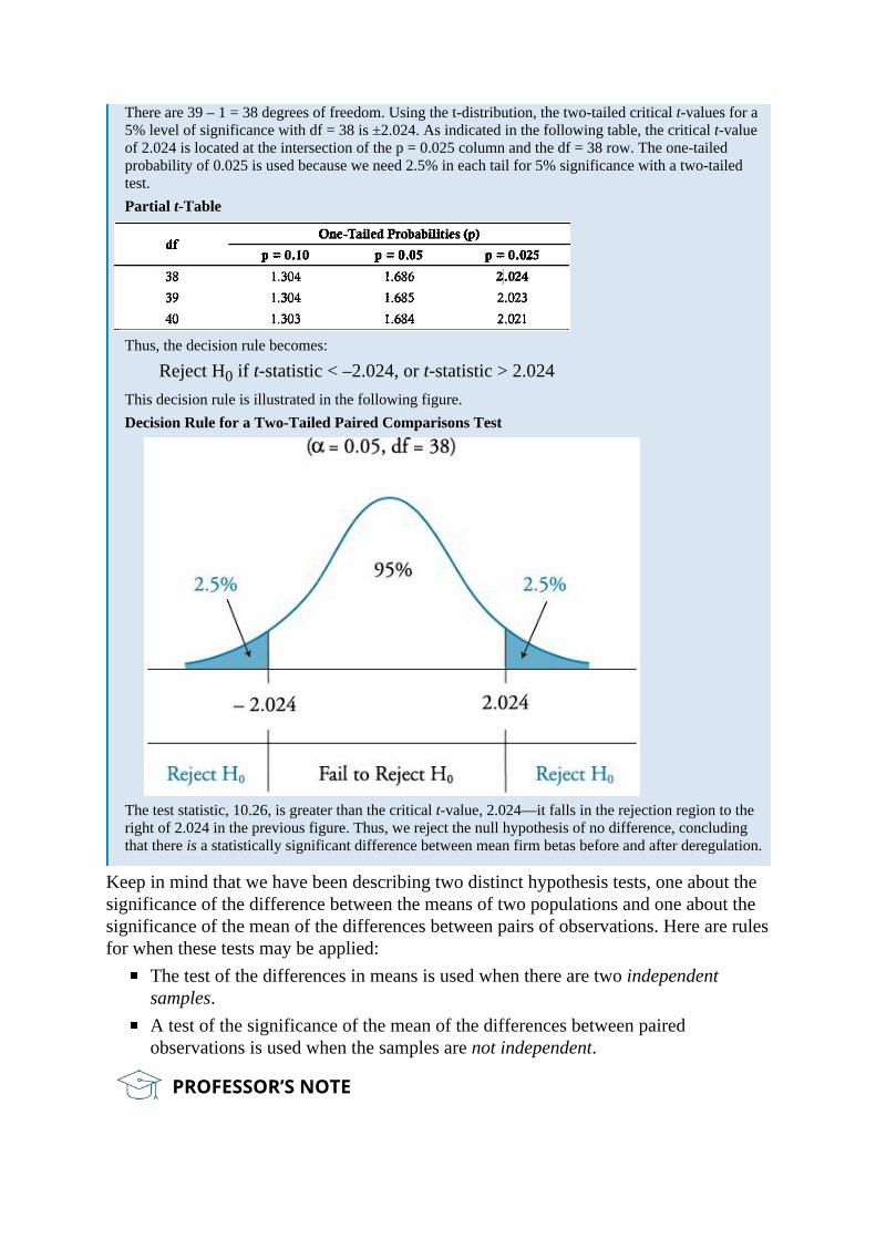
There are 39 – 1 = 38 degrees of freedom. Using the t-distribution, the two-tailed critical t-values for a5% level of significance with df = 38 is ±2.024. As indicated in the following table, the critical t-valueof 2.024 is located at the intersection of the p = 0.025 column and the df = 38 row. The one-tailedprobability of 0.025 is used because we need 2.5% in each tail for 5% significance with a two-tailedtest.Partial t-Table

Thus, the decision rule becomes:

Reject H0 if t-statistic < –2.024, or t-statistic > 2.024This decision rule is illustrated in the following figure.Decision Rule for a Two-Tailed Paired Comparisons Test

The test statistic, 10.26, is greater than the critical t-value, 2.024—it falls in the rejection region to theright of 2.024 in the previous figure. Thus, we reject the null hypothesis of no difference, concludingthat there is a statistically significant difference between mean firm betas before and after deregulation.

Keep in mind that we have been describing two distinct hypothesis tests, one about thesignificance of the difference between the means of two populations and one about thesignificance of the mean of the differences between pairs of observations. Here are rulesfor when these tests may be applied:

The test of the differences in means is used when there are two independentsamples.A test of the significance of the mean of the differences between pairedobservations is used when the samples are not independent.

PROFESSOR’S NOTE

The LOS here say “Identify the appropriate test statistic and interpret the results...” I can’tbelieve candidates are expected to memorize these formulas (or that you would be a betteranalyst if you did). You should instead focus on the fact that both of these tests involve t-statistics and depend on the degrees of freedom. Also note that when samples areindependent, you can use the difference in means test, and when they are dependent, we mustuse the paired comparison (mean differences) test. In that case, with a null hypothesis thatthere is no difference in means, the test statistic is simply the mean of the differencesbetween each pair of observations, divided by the standard error of those differences.

LOS 12.j: Identify the appropriate test statistic and interpret the results for ahypothesis test concerning 1) the variance of a normally distributed population,and 2) the equality of the variances of two normally distributed populations basedon two independent random samples.

CFA® Program Curriculum, Volume 1, page 646The chi-square test is used for hypothesis tests concerning the variance of a normallydistributed population. Letting σ2 represent the true population variance and represent the hypothesized variance, the hypotheses for a two-tailed test of a singlepopulation variance are structured as:

The hypotheses for one-tailed tests are structured as:

H0: σ2 ≤ versus Ha: σ2 >, or

H0: σ2 ≥ versus Ha: σ2 <

Hypothesis testing of the population variance requires the use of a chi-square distributedtest statistic, denoted χ2. The chi-square distribution is asymmetrical and approaches thenormal distribution in shape as the degrees of freedom increase.To illustrate the chi-square distribution, consider a two-tailed test with a 5% level ofsignificance and 30 degrees of freedom. As displayed in Figure 12.7, the critical chi-square values are 16.791 and 46.979 for the lower and upper bounds, respectively.These values are obtained from a chi-square table, which is used in the same manner asa t-table. A portion of a chi-square table is presented in Figure 12.8.Note that the chi-square values in Figure 12.8 correspond to the probabilities in the righttail of the distribution. As such, the 16.791 in Figure 12.7 is from the column headed0.975 because 95% + 2.5% of the probability is to the right of it. The 46.979 is from thecolumn headed 0.025 because only 2.5% probability is to the right of it. Similarly, at a5% level of significance with 10 degrees of freedom, Figure 12.8 shows that the criticalchi-square values for a two-tailed test are 3.247 and 20.483.

Figure 12.7: Decision Rule for a Two-Tailed Chi-Square Test

Figure 12.8: Chi-Square Table

The chi-square test statistic, χ2, with n − 1 degrees of freedom, is computed as:

where:n = sample sizes2 = sample variance

= hypothesized value for the population variance.Similar to other hypothesis tests, the chi-square test compares the test statistic, , toa critical chi-square value at a given level of significance and n − 1 degrees of freedom.Note that since the chi-square distribution is bounded below by zero, chi-square valuescannot be negative.

EXAMPLE: Chi-square test for a single population variance

Historically, High-Return Equity Fund has advertised that its monthly returns have a standard deviationequal to 4%. This was based on estimates from the 2005–2013 period. High-Return wants to verifywhether this claim still adequately describes the standard deviation of the fund’s returns. High-Returncollected monthly returns for the 24-month period between 2013 and 2015 and measured a standarddeviation of monthly returns of 3.8%. High-Return calculates a test statistic of 20.76. Using a 5%significance level, determine if the more recent standard deviation is different from the advertisedstandard deviation.Answer:The null hypothesis is that the standard deviation is equal to 4% and, therefore, the variance of monthlyreturns for the population is (0.04)2 = 0.0016. Since High-Return simply wants to test whether thestandard deviation has changed, up or down, a two-sided test should be used. The hypothesis teststructure takes the form:

The appropriate test statistic for tests of variance is a chi-square statistic.With a 24-month sample, there are 23 degrees of freedom. Using the table of chi-square values inAppendix E at the back of this book, for 23 degrees of freedom and probabilities of 0.975 and 0.025,we find two critical values, 11.689 and 38.076. Thus, the decision rule is:

Reject H0 if χ2 < 11.689, or χ2 > 38.076This decision rule is illustrated in the following figure.Decision Rule for a Two-Tailed Chi-Square Test of a Single Population Variance

Since the computed test statistic, χ2, falls between the two critical values, we cannot reject the nullhypothesis that the variance is equal to 0.0016. The recently measured standard deviation is closeenough to the advertised standard deviation that we cannot say that it is different from 4%, at a 5%level of significance.

Testing the Equality of the Variances of TwoNormally Distributed Populations, Based on Two

Independent Random SamplesThe hypotheses concerned with the equality of the variances of two populations aretested with an F-distributed test statistic. Hypothesis testing using a test statistic thatfollows an F-distribution is referred to as the F-test. The F-test is used under theassumption that the populations from which samples are drawn are normally distributedand that the samples are independent.If we let and represent the variances of normal Population 1 and Population 2,respectively, the hypotheses for the two-tailed F-test of differences in the variances canbe structured as:

and the one-sided test structures can be specified as:

The test statistic for the F-test is the ratio of the sample variances. The F-statistic iscomputed as:

where: = variance of the sample of n1 observations drawn from Population 1 = variance of the sample of n2 observations drawn from Population 2

Note that n1 − 1 and n2 − 1 are the degrees of freedom used to identify the appropriatecritical value from the F-table (provided in the Appendix).

PROFESSOR’S NOTE

Always put the larger variance in the numerator ( ). Following this convention means weonly have to consider the critical value for the right-hand tail.

An F-distribution is presented in Figure 12.9. As indicated, the F-distribution is right-skewed and is bounded by zero on the left-hand side. The shape of the F-distribution isdetermined by two separate degrees of freedom, the numerator degrees of freedom, df1,and the denominator degrees of freedom, df2.

Figure 12.9: F-Distribution

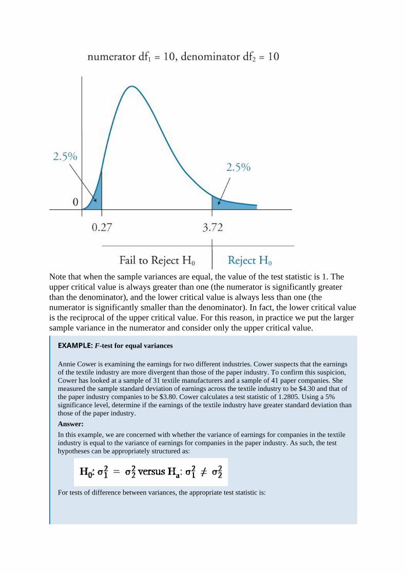
Note that when the sample variances are equal, the value of the test statistic is 1. Theupper critical value is always greater than one (the numerator is significantly greaterthan the denominator), and the lower critical value is always less than one (thenumerator is significantly smaller than the denominator). In fact, the lower critical valueis the reciprocal of the upper critical value. For this reason, in practice we put the largersample variance in the numerator and consider only the upper critical value.

EXAMPLE: F-test for equal variances

Annie Cower is examining the earnings for two different industries. Cower suspects that the earningsof the textile industry are more divergent than those of the paper industry. To confirm this suspicion,Cower has looked at a sample of 31 textile manufacturers and a sample of 41 paper companies. Shemeasured the sample standard deviation of earnings across the textile industry to be $4.30 and that ofthe paper industry companies to be $3.80. Cower calculates a test statistic of 1.2805. Using a 5%significance level, determine if the earnings of the textile industry have greater standard deviation thanthose of the paper industry.Answer:In this example, we are concerned with whether the variance of earnings for companies in the textileindustry is equal to the variance of earnings for companies in the paper industry. As such, the testhypotheses can be appropriately structured as:

For tests of difference between variances, the appropriate test statistic is:

where is the larger sample variance.

Using the sample sizes for the two industries, the critical F-value for our test is found to be 1.94. Thisvalue is obtained from the table of the F-distribution for 2.5% in the upper tail, with df1 = 30 and df2 =40. Thus, if the computed F-statistic is greater than the critical value of 1.94, the null hypothesis isrejected. The decision rule, illustrated in the following figure, can be stated as:

Reject H0 if F > 1.94Decision Rule for F-Test

Since the calculated F-statistic of 1.2805 is less than the critical F-statistic of 1.94, Cower cannot rejectthe null hypothesis. Cower should conclude that the earnings variances of the industries are notsignificantly different from one another at a 5% level of significance.

LOS 12.k: Distinguish between parametric and nonparametric tests and describesituations in which the use of nonparametric tests may be appropriate.

CFA® Program Curriculum, Volume 1, page 652Parametric tests rely on assumptions regarding the distribution of the population andare specific to population parameters. For example, the z-test relies upon a mean and astandard deviation to define the normal distribution. The z-test also requires that eitherthe sample is large, relying on the central limit theorem to assure a normal samplingdistribution, or that the population is normally distributed.Nonparametric tests either do not consider a particular population parameter or havefew assumptions about the population that is sampled. Nonparametric tests are used

when there is concern about quantities other than the parameters of a distribution orwhen the assumptions of parametric tests can’t be supported. They are also used whenthe data are not suitable for parametric tests (e.g., ranked observations).Situations where a nonparametric test is called for are the following:

1. The assumptions about the distribution of the random variable that support aparametric test are not met. An example would be a hypothesis test of the meanvalue for a variable that comes from a distribution that is not normal and is ofsmall size so that neither the t-test nor the z-test is appropriate.

2. When data are ranks (an ordinal measurement scale) rather than values.3. The hypothesis does not involve the parameters of the distribution, such as testing

whether a variable is normally distributed. We can use a nonparametric test, calleda runs test, to determine whether data are random. A runs test provides an estimateof the probability that a series of changes (e.g., +, +, –, –, +, –,….) are random.

The Spearman rank correlation test can be used when the data are not normallydistributed. Consider the performance ranks of 20 mutual funds for two years. The ranks(1 through 20) are not normally distributed, so a standard t-test of the correlations is notappropriate. A large positive value of the Spearman rank correlations, such as 0.85,would indicate that a high (low) rank in one year is associated with a high (low) rank inthe second year. Alternatively, a large negative rank correlation would indicate that ahigh rank in year 1 suggests a low rank in year 2, and vice versa.

MODULE QUIZ 12.3

To best evaluate your performance, enter your quiz answers online.

1. Which of the following assumptions is least likely required for the difference inmeans test based on two samples?

A. The two samples are independent.B. The two populations are normally distributed.C. The two populations have equal variances.

2. William Adams wants to test whether the mean monthly returns over the last fiveyears are the same for two stocks. If he assumes that the returns distributionsare normal and have equal variances, the type of test and test statistic are bestdescribed as:

A. paired comparisons test, t-statistic.B. paired comparisons test, F-statistic.C. difference in means test, t-statistic.

3. Which of the following statements about the F-distribution and chi-squaredistribution is least accurate? Both distributions:

A. are asymmetrical.B. are bounded by zero on the left.C. have means that are less than their standard deviations.

4. The appropriate test statistic for a test of the equality of variances for twonormally distributed random variables, based on two independent randomsamples, is:

A. the t-test.B. the F-test.C. the χ2 test.

5. The appropriate test statistic to test the hypothesis that the variance of anormally distributed population is equal to 13 is:

A. the t-test.B. the F-test.C. the χ2 test.

KEY CONCEPTSLOS 12.aThe hypothesis testing process requires a statement of a null and an alternativehypothesis, the selection of the appropriate test statistic, specification of the significancelevel, a decision rule, the calculation of a sample statistic, a decision regarding thehypotheses based on the test, and a decision based on the test results.The null hypothesis is what the researcher wants to reject. The alternative hypothesis iswhat the researcher wants to support, and it is accepted when the null hypothesis isrejected.

LOS 12.bA two-tailed test results from a two-sided alternative hypothesis (e.g., Ha: µ ≠ µ0). Aone-tailed test results from a one-sided alternative hypothesis (e.g., Ha: µ > µ0, or Ha: µ< µ0).

LOS 12.cThe test statistic is the value that a decision about a hypothesis will be based on. For atest about the value of the mean of a distribution:

A Type I error is the rejection of the null hypothesis when it is actually true, while aType II error is the failure to reject the null hypothesis when it is actually false.The significance level can be interpreted as the probability that a test statistic will rejectthe null hypothesis by chance when it is actually true (i.e., the probability of a Type Ierror). A significance level must be specified to select the critical values for the test.

LOS 12.dHypothesis testing compares a computed test statistic to a critical value at a stated levelof significance, which is the decision rule for the test.The power of a test is the probability of rejecting the null when it is false. The power ofa test = 1 − P(Type II error).A hypothesis about a population parameter is rejected when the sample statistic liesoutside a confidence interval around the hypothesized value for the chosen level ofsignificance.

LOS 12.eStatistical significance does not necessarily imply economic significance. Even though atest statistic is significant statistically, the size of the gains to a strategy to exploit astatistically significant result may be absolutely small or simply not great enough tooutweigh transactions costs.

LOS 12.f

The p-value for a hypothesis test is the smallest significance level for which thehypothesis would be rejected. For example, a p-value of 7% means the hypothesis canbe rejected at the 10% significance level but cannot be rejected at the 5% significancelevel.

LOS 12.gWith unknown population variance, the t-statistic is used for tests about the mean of anormally distributed population: . If the population variance is known, the

appropriate test statistic is for tests about the mean of a population.

LOS 12.hFor two independent samples from two normally distributed populations, the differencein means can be tested with a t-statistic. When the two population variances areassumed to be equal, the denominator is based on the variance of the pooled samples,but when sample variances are assumed to be unequal, the denominator is based on acombination of the two samples’ variances.

LOS 12.iA paired comparisons test is concerned with the mean of the differences between thepaired observations of two dependent, normally distributed samples. A t-statistic,

, where , and d is the average difference of the n paired observations, is

used to test whether the means of two dependent normal variables are equal. Valuesoutside the critical t-values lead us to reject equality.

LOS 12.jThe test of a hypothesis about the population variance for a normally distributed

population uses a chi-square test statistic: , where n is the sample size, s2

is the sample variance, and is the hypothesized value for the population variance.Degrees of freedom are n − 1.

The test comparing two variances based on independent samples from two normally

distributed populations uses an F-distributed test statistic: , where is the

variance of the first sample and is the (smaller) variance of the second sample.

LOS 12.kParametric tests, like the t-test, F-test, and chi-square tests, make assumptions regardingthe distribution of the population from which samples are drawn. Nonparametric testseither do not consider a particular population parameter or have few assumptions aboutthe sampled population. Nonparametric tests are used when the assumptions ofparametric tests can’t be supported or when the data are not suitable for parametric tests.

ANSWER KEY FOR MODULE QUIZZES

Module Quiz 12.1

1. C To test whether the population mean is greater than 20, the test would attemptto reject the null hypothesis that the mean is less than or equal to 20. The nullhypothesis must always include the “equal to” condition. (LOS 12.a)

2. C Rejecting the null when it is actually true is a Type I error. A Type II error isfailing to reject the null hypothesis when it is false. The significance level equalsthe probability of a Type I error. (LOS 12.b, 12.c)

3. C A Type I error is rejecting the null hypothesis when it’s true. The probability ofrejecting a false null is [1 − Prob Type II] = [1 − 0.60] = 40%, which is called thepower of the test. A and B are not necessarily true, since the null may be false andthe probability of rejection unknown. (LOS 12.c)

4. A The power of a test is 1 − P(Type II error) = 1 − 0.15 = 0.85. (LOS 12.d)

Module Quiz 12.2

1. B With a p-value of 3%, the manager can reject the null hypothesis (that abnormalreturns are less than or equal to zero) using a significance level of 3% or higher.Although the test result is statistically significant at significance levels as small as3%, this does not necessarily imply that the result is economically meaningful.(LOS 12.e, 12.f)

2. A With a small sample size, a t-test may be used if the population isapproximately normally distributed. If the population has a nonnormaldistribution, no test statistic is available unless the sample size is large. (LOS12.g)

3. B This is a two-tailed test with 14 – 1 = 13 degrees of freedom. From the t-table,2.160 is the critical value to which the analyst should compare the calculated t-statistic. (LOS 12.g)

Module Quiz 12.3

1. C When the variances are assumed to be unequal, we just calculate thedenominator (standard error) differently and use both sample variances tocalculate the t-statistic. (LOS 12.h)

2. A Since the observations are likely dependent (both related to market returns), apaired comparisons (mean differences) test is appropriate and is based on a t-statistic. (LOS 12.h, 12.i)

3. C There is no consistent relationship between the mean and standard deviation ofthe chi-square distribution or F-distribution. (LOS 12.j)

4. B The F-test is the appropriate test. (LOS 12.j)

5. C A test of the population variance is a chi-square test. (LOS 12.j)