using slamm to better understand sea level rise on the ... · using slamm to better understand sea...
TRANSCRIPT
Page 1 of 29
Using SLAMM to better understand Sea Level Rise on the Francis Marion National Forest
GIS Capstone Project http://arcg.is/2a6V1qO
Chelsea Leitz CP 6950
Page 2 of 29
Table of Contents
Abstract …3
Introduction …3
Literature Review …4
Data …10
Method …10
Results …16
Obstacles …17
Conclusions …18
References …19
Appendices …20
Page 3 of 29
Abstract
How is sea level rise influencing the ecosystems and related management? This paper
will discuss the examining of the Francis Marion National Forest via SLAMM & Satellite
Imagery to better understand the sea level rise influence on ecosystems and to better related
Coastal Management Decisions. Running the Sea Level Affecting Marshes Model will allow for
users to understand where there will be potential changes in the seascape and how to prepare for
these locations and formulate restoration processes for the future. Can increased sea level and
salinity intrusion amplify coastal drought possibilities and could it be an indicator for increased
fires? This model will help answer these types of questions. Exhausting this model coupled with
satellite imagery for comparison purposes will allow for further awareness of the effects of
increased tidal flooding and how the forest can plan for these potential problems.
Introduction/Background
Within the past few decades, GIS has become much more prevalent in Coastal
Management. Using geospatial technology to investigate terrestrial landscapes has been around
for much longer and only as of late, has it been recognized as a vital part of understanding our
coastal communities. The technology matured with its focus on the land; however, coastal
habitats are entirely different and those methods and procedures cannot simply be applied to a
completely different environment. Therefore, more aquatic based models and tools have been
created specifically with understanding our coasts.
The Sea Level Affecting Marshes Model (SLAMM) is a simulation of wetlands and
shore line changes during a long term sea level rise. The model uses digital elevation data and
can incorporate various parameters ranging from impervious surfaces, salinities, dike locations,
Page 4 of 29
and more to determine where sea level rise will be an impact. Combining the results of this
model with change detection analysis from Landsat 8 images will allow for understanding of the
past, which will help in confirming the predictions are practical.
The following paper will examine related literature, SLAMM’s results and expectations
for the Francis Marion National Forest, change detection analysis results, and the anticipated
changes from both methods. The effectiveness of the model for future uses in predicting changes
in order to provide support for the Forest Plan will also be investigated. Coastal Management
needs to be improved and if a model can help provide evidence for better policies, then it should
be utilized fully.
Literature Review
The following articles are areas of research that support my project. They range from the
basics of using GIS for Coastal Managements, to background on the Francis Marion Forest, as
well as specific studies using similar models in different coastal regions. Each source of
information relates back to why studying wetland growth in coastal regions is essential and how
to better convey that significance to coastal resource managers.
• Geographic Information Systems applied to Integrated Coastal Zone Management:
o This paper focuses on the overall benefits of using GIS for coastal zone
management. Coastal zones provide vital social, economic, and environmental
resources; in order to better manage these areas, changes need to be prepared for
with mitigation policies in place. However, evidence for policies comes from
scientific studies. Using GIS to provide that evidence is undeniably the best
course of direction. Within the coastal environments, the littoral areas,and the
interactions of marine and terrestrial processes, need to be understood better.
Since GIS specifics the spatial and temporal dynamic processes and their
evolutions, it is the best tool. This paper provides three applications of GIS: “1) In
Page 5 of 29
coastal hazards management GIS helps with statistics analysis, needed to carry
out a multivariate spatial-temporal model that estimates the probability of a
hazard occurrence; 2) Dealing with shorelines corresponding to different years,
GIS allows the analysis of evolutionary trends to define the behavior of the
system; 3) GIS used in studies of the evolution of dune fields is essential in order
to estimate dune migration rates and analyze all the variables involved in this
process” (CoastGIS 101).
o The first application discusses the many factors involved in studying coastal
hazards in the Mediterranean Sea. To determine the safety of the coastal
waterfronts, elevation, swell information, streams, rock fall occurrences from
cliffs, erosion and human impacts are all necessary data sets. With GIS, modeling
the data to map the unstable areas and to determine the at risk elements is much
easier. Vulnerability zones can be mapped by overlapping the hazard maps and
the at risk maps. From those analyses, decision support systems can be
implemented.
o GIS can also understand shoreline evolution by comparing previous cartographic
data. Determine coastal changes with current imagery allows for the
understanding of flooding and sea level rises. Additionally sand dune transitions
can also be determined. Specifically, data sets related to wind transport, swell,
sediments can all be incorporated into the geodatabase as well as field survey
data.
o This paper concludes that GIS implementation is still a new and growing field,
but can be vital in supporting policies by providing spatial, visual, and statistical
analysis. Land management has utilized GIS more so than coastal environments
and that needs to change.
• Francis Marion National Forest –Draft Final Environmental Impact Statement
o Every ten years, the National Forest revise their Land and Resource Management
Plan for each individual forest
o For the expected 2016 Francis Marion Forest Plan, there is more emphasis on
understanding climate changes effects on various aspects of the forest,
specifically coastal ecosystems. There already has been rises in sea levels and
Page 6 of 29
intense storms such as Hurricane Hugo, which nearly decimated the entire forest.
It is vital to understand that “as saltwater flooding expands, low-lying coastal wet
forest could become marshland where land-use barriers do not exist (Ervin et al.,
2006). Tidal forests, including bald cypress swamps, may serve as sentinels for
sea-level rise do to their low tolerance to salinity changes” (78). These tidal
forests provide habitats for many wildlife species including endangered storks
nesting in cypress swamps.
o Saltwater intrusion: Sea level rise will increase the potential for saltwater
intrusion into coastal freshwater tables and ground waters. Collaboration with
local municipalities is needed to monitor saltwater intrusion.
o Using SLAMM and imagery can provide evidence for better policies to include in
the next Forest Plan. Using models and images can detect changes and can
incorporate where restoration procedures will need to take place.
• Drought and Coastal Ecosystems: An Assessment of Decision Maker Needs for
Information Fifth Interagency Conference on Research in the Watersheds: Kirsten
Lackstrom, Amanda Brennan, Kirstin Dow - Carolinas Integrated Sciences &
Assessments, University of South Carolina
o This research program emphasizes the necessity of understanding coastal
droughts and its differences as an ecological drought. The Coastal Carolinas
experience these droughts due to freshwater deficiency and salt water intrusion
from tidal flooding, both causing stress on the habitats and species. Their goals
are to understand how and what to monitor and to develop mitigation strategies.
o The research included interviewing recreational and commercial fisheries,
recreation businesses, and land/refuge managers. These interviews defined the
drought as changes in the availability and timing of freshwater, changes in water
quality with increasing salinity and fluctuations.
o The goal is to understand the impacts of the coastal drought. Beyond the direct
physical impacts, what species and ecosystems are effected, what other stressors
can be an issues (climate, human, biological), then how will the individuals and
organizations be effected and what will the adaption responses be? Additionally, a
Page 7 of 29
drought early warning system would be extremely helpful. To understand the
salinity effects, the seasonal changes, the normal/baseline would be beneficial to
all parties involved. Coastal droughts do exist and to be able to predict the
increase flow of salt water can be done by SLAMM, then providing locations and
potentials of coastal drought.
• Sea-level rise and drought interactions accelerate forest decline on the Gulf Coast of
Florida, USA: Larisa R. G Desantis, Smriti Bhotika, Kimberlyn Williams, and Francis E.
Putz
o This study in Florida acknowledges that increased tidal flooding contributes to the
“well documented decline of species-rich coastal forest areas along the Gulf of
Mexico” (2349). While this study did not focus on using spatial and GIS
technology for analysis, it did concentration on the specific species affected by
tidal flooding and the increase of salinity’s effects on their habitats. The recent
rates of sea level rise along the Gulf Coast can be as high as 11.9mm/yr. These
saltwater “intrusions cause reduced canopy tree regeneration, declines in over
story tree species diversity.
o Florida has low elevations and flat topography, making it vulnerable to shoreline
changes and retreats. The specific area of study in Waccasassa Bay Preserve State
Park included multiple study plots of 20m x 20m. Within these plots, live tree
species such as cabbage palm, southern red cedar, live oak, and sugarberry and
others were tagged and mapped in the early nineties and early two thousands. This
survey style of research differs from my own, but provides recognition of past
changes based on field data. The trees examined in this study similarly grow in
the Francis Marion Forest in South Carolina. Acknowledging a study that
determined changes in tree growth from salt water intrusion in the past will
provide coastal resource management with evidence to conduct similar studies as
my own to predict the future problem and drought areas. Heights and diameters of
the trees were measured as well as the forest health, which includes stable isotype
analysis “to investigate uptake if fresh ground water” (2350).
o The method of the analysis included comparing tree survivorship from the early
1990s to the expected surviving trees in 2005. Their sea-level rise data was
Page 8 of 29
calculated based on the Cedar Key Station from 1939-2005. La Nina events were
included as well as weather data acquired from the Tampa Airport, leading to an
average rate of 2.4mm/yr. The isotope analysis was collected using tree trunk
cores. The sample was examined in a mass spectrometer to determine those
oxygen and hydrogen values. Leaf samples were also examined to determine
water stress.
o The results of their study determined that coastal forests declined in species
richness, the lower the elevations and the increasing flooding frequency. After
2005, the disappearance of the S. palmetto was in the most regularly flooding
plot. The tree remained in plots with less than 26 weeks of tidal flooding.
Additionally, regeneration of species declined in these frequently flooded plot as
well as density. Using the weather data regarding La Nina, the effects of sea level
rise were more intense during those drought times.
o The study determined that tree species were affected negatively by tidal flooding
events and salt water intrusions. Some species are more tolerant of the higher
salinity, but their regeneration rates are not consistent. Using these lab and field
studies, exposure to salt will effect tree species and their regeneration. Knowing
this information helps provide significant reasons to perform predictive analysis
tests in a format similar to my research. Using a model to predict flooding based
on the past sea level rise will indicate the areas of salt water intrusion as well as
potential coastal drought and fires.
• Application of the Sea-Level Affecting Marshes Model (SLAMM 5.0.2) in the Lower
Delmarva Peninsula - Northampton and Accomack counties, VA, -Somerset and
Worcester counties, MD: By Delissa Padilla Nieves, Conservation Biology Program,
National Wildlife Refuge System, Arlington, VA
o This study focuses on the Delmarva Peninsula, along the eastern shore of Virginia
and Maryland. This region includes barriers islands as well as the mainland, with
coastal reserves and national wildlife refuges. Land types include beach, dunes,
freshwater swells, maritime forest, marshes, and tidal flats all providing habitats
for migratory birds and other species.
Page 9 of 29
o This study area is similar to the Francis Marion National Forest study area since
both include areas of wildlife refuges as well as a range in habitats from barrier
islands to swamps, marshes and forests. Both regions experience frequent
interactions with storms, storm surge, waves and wind. The differences are the
extreme overwash that Assateague experiences, causing sediment transportation.
o This study uses expected sea level rise trends from NOAA’s tides and currents
website, the same source for my own study. Their goals are to project the effects
of sea level rise on the coastal habitats, specifically within the wildlife refuges.
o “Within SLAMM, there are five primary processes that affect wetland fate under
different scenarios of sea-level rise:
Inundation: The rise of water levels and the salt boundary is tracked by
reducing elevations of each cell as sea levels rise, thus keeping mean tide
level constant at zero.
Erosion: Erosion is triggered based on a threshold of maximum fetch and the
proximity of the wetland to estuarine water or Open Ocean.
Overwash: Beach migration and transport of sediments are calculated based
on storm frequency.
Saturation: Coastal swamps and fresh marshes can migrate onto adjacent
uplands as a response to a rise in the water table
Accretion: Sea-level rise is offset by sedimentation and vertical accretion
using average or site-specific values for each wetland category.
SLAMM integrates localized conditions of sea-level rise, wetland elevation
changes (accretion and submergence), and wave-action erosion to simulate
wetland conversions. Therefore, relative sea-level rise is estimated based on
site-specific conditions” (6).
Similar to my study, GIS was used to process the data for the model.
Elevation data is from the USGS NED, SLAMM codes were assigned to the
National Wetlands Inventory Data, from the US Fish & Wildlife Inventory.
The impervious surfaces data was from the National Land Cover Database
2001. All data was used at a 30m by 30, cell size. The climate scenarios they
used included the A1B, 1 meter rise and 1.5 meter rise in 25 year increments
starting at the NWI photo date until 2100.
Page 10 of 29
As mentioned previously, one of the differences between this SLAMM study
and my own was Assateague’s overwash issues. They accounted for this
within the model by adjusting the default values to maximum width of the
barrier island as well as including previous overwash events and by how
much.
The conclusion of their study reiterated the growth of wetlands and change of
the shorelines. Wetlands were projected to convert to open water in some
areas and migration of wetlands is anticipated on the other shores. The
irregularly flooded marshes are expected to be the most impacted with a
potential loss of 68%-91% for brackish and 37%-49% decline in salt marsh.
Fresh tidal marshes are expected losses of 73%. The estuarine beaches
expected gains in all their tested scenarios. Their major obstacles with the
model is the lack of simple formulas for the overwash events in the barrier
islands.
Data
This study has three required data sets. The digital evaluation data is 10 foot Spatial
Resolution for Francis Marion Ranger District 2009 LiDAR. The slope is required and that is
derived from the DEM. The National Wetlands Inventory provides the wetlands polygon
shapefiles from the Fish & Wildlife Service. These are organized by types of wetlands and the
surrounding land types. The average sea level rise data was collected from NOAA’s Tides and
Currents websites. The sea level trends are collected at various stations along the coast. For this
study, I used the average of the Myrtle Beach and Charleston stations. Unfortunately there was
not expansive historical data specifically for the Francis Marion National Forest, so the average
of these two stations, both within 50 miles will suffice. For more extensive studies, there are
various other parameters that can be applied such as the impervious surfaces, from the National
Land Cover Datasets, Tidal Datum, historical erosion and accretion rates as well as beach
sedimentation rates.
Page 11 of 29
For my comparison purposes, I analyzed Landsat images expanding over Berkley and
Charleston counties. The images are derived from the USDA National Agriculture Imagery
Program (NAIP) taken during the growing seasons “leaf-on” throughout the U.S. The images are
acquired at 1 meter ground distance with a spectral resolution at natural color (red, green and
blue). Additionally, each image should have less than 10% of cloud cover.
For reference purposes, I acquired the SLAMM 3.0 Version outputs of a similar study
area. This previous study used 0.4 meter rise on the Cape Romain Wildlife Refuge. This area is
slightly southeast of my study site and it includes more marsh lands and barrier islands.
However, this data provides good background on how the model functioned at the 3.0 version
and a reference point for my results.
Methods
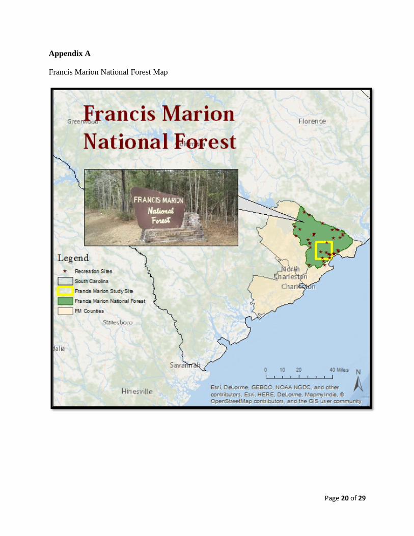
Study Area:
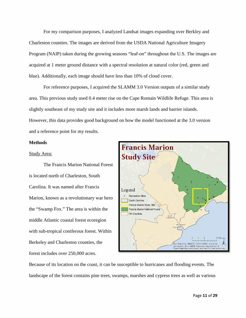
The Francis Marion National Forest
is located north of Charleston, South
Carolina. It was named after Francis
Marion, known as a revolutionary war hero
the “Swamp Fox.” The area is within the
middle Atlantic coastal forest ecoregion
with sub-tropical coniferous forest. Within
Berkeley and Charleston counties, the
forest includes over 250,000 acres.
Because of its location on the coast, it can be susceptible to hurricanes and flooding events. The
landscape of the forest contains pine trees, swamps, marshes and cypress trees as well as various
Page 12 of 29
wildlife, such as the endangered red-cockaded woodpecker. Blocking direct access to the
Atlantic Ocean is Cape Romain, the National Wildlife Refuge that includes marshes, creeks, and
barrier islands, mostly accessible by boat only.
Model:
Sea Level Affecting Marshes Model (SLAMM) is a program initially funded by the EPA
to provide details about coastal habitats in response to Sea Level Rise. The model can provide
various outputs of sea level rise and the potential conflicts within coastal environments. The six
main processes of the model are inundation, erosion, accretion, saturation, overwash and salinity.
The required inputs include the digital elevation models and its resulting slope, as well as the
national wetlands inventory converted to SLAMM codes. Additionally, the user has the choice of
various sea level rise scenarios, ranging from 0.4 to 1.5 meters by 2100, or using the IPCC
scenarios of A1, A2, B1, or B2. “Within SLAMM, there are five primary processes that affect
wetland fate under different scenarios of sea-level rise:
Inundation: The rise of water levels and the salt boundary is tracked by reducing
elevations of each cell as sea levels rise, thus keeping mean tide level constant at zero.
Erosion: Erosion is triggered based on a threshold of maximum fetch and the proximity
of the wetland to estuarine water or Open Ocean.
Overwash: Beach migration and transport of sediments are calculated based on storm
frequency.
Saturation: Coastal swamps and fresh marshes can migrate onto adjacent uplands as a
response to a rise in the water table
Accretion: Sea-level rise is offset by sedimentation and vertical accretion using average
or site-specific values for each wetland category.
SLAMM integrates localized conditions of sea-level rise, wetland elevation changes (accretion
and submergence), and wave-action erosion to simulate wetland conversions. Therefore, relative
sea-level rise is estimated based on site-specific conditions” (Polaczyk, 2013).
Page 13 of 29
Pre-Processing:
In order to run the model, there are three required datasets, DEM, Slope, and NWI. The
10ft DEM was obtained from the Forest Service from 2009 LiDAR data. It was then used to
create the slope raster by the spatial statistic tool. The cell size of every raster was 10 by 10,
based on the initial elevation model. All files are projected NAD 1983 State Plane South
Carolina FIPS 3900 Feet Intl. These files were initially the original boundaries of the Francis
Marion Forest, but for the sake of time, everything was clipped to the North portion of
Charleston County, SC. This study site included a portion of the open water, river, and marshes
as well as an extensive forest section. Both the DEM and slope were then converted to ASCII
using ESRI’s tool, raster to ASCII. The National Wetlands Inventory was downloaded from their
website owned by the Fish & Wildlife Agency. In order for the model to recognize the wetlands
code categories, they need to be converted to SLAMM codes. The table and description of codes
is within the Appendix. The polygon file of South Carolina was clipped to the Berkley and
Charleston Counties. This file was then converted to a raster based on the SLAMM code values.
The raster to ASCII tool was also used for the wetlands raster. For the initial test run, the data
was also clipped to a smaller Northern portion of Charleston County.
Sea Level trends have been on the rise in the recorded years. For this study, I ran the
model for two different scenarios. The first is an average of the Sea Level Rise Trends values
collected from two stations north & south of the forest. The Francis Marion sits between two
stations on the east coast, the Myrtle Beach station and the Charleston Station. In Myrtle Beach,
“The mean sea level trend is 3.9 mm/year with a 95% confidence interval of +/- 0.58 mm/year
based on monthly mean sea level data from 1957 to 2015 which is equivalent to a change of 1.28
feet in 100 years” (NOAA Tides & Currents). While in Charleston, “The mean sea level trend is
Page 14 of 29
3.21 mm/year with a 95% confidence interval of +/- 0.22 mm/year based on monthly mean sea
level data from 1921 to 2015 which is equivalent to a change of 1.05 feet in 100 years” (NOAA
Tides & Currents). For my purposes, I am taking the average of the two stations, which is
3.55mm/year. Based on these values, by 2025, there will be a 35.5mm increase. By 2050, there
will be a 124.25mm increase, roughly 1/8th of a meter. These values certainly are not the worst
case scenarios available, but rather estimates based on the past 60-80 years. Since the future is
always uncertain, this study will focus just on the historical recorded values for the nearby
areas.
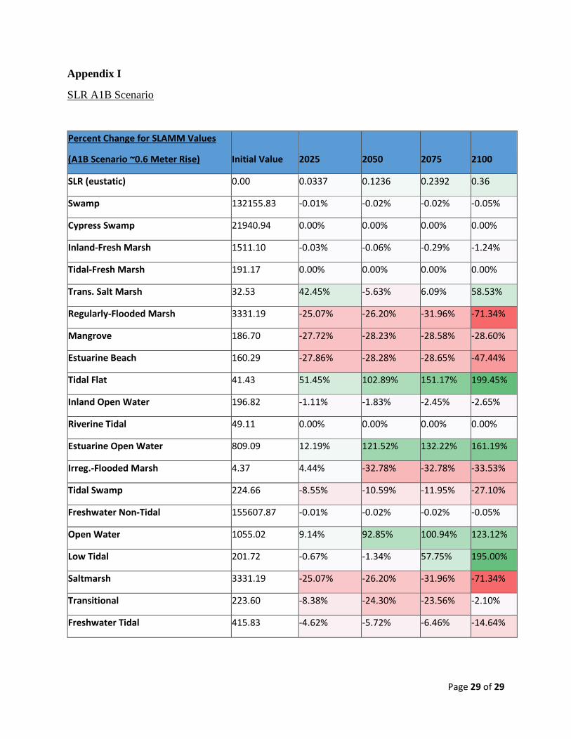
The second scenario is the A1B Climate Change Scenario from the International Panel of
Climate Change. This environment “describes a future world of very rapid economic growth,
global population that peaks in mid-century and declines thereafter, and the rapid introduction of
new and more efficient technologies. Major underlying themes are convergence among regions,
capacity building and increased cultural and social interactions, with a substantial reduction in
regional differences in per capita income. The three A1 groups are distinguished by their
technological emphasis: fossil intensive (A1FI), non-fossil energy sources (A1T), or a balance
across all sources (A1B) (where balanced is defined as not relying too heavily on one particular
energy source, on the assumption that similar improvement rates apply to all energy supply and
end-use technologies)” (IPCC, 2016).
Execution
Running the model included a few steps. To avoid any errors and a successful run, each
input needs to be the same cell extent. Once all input are uploaded to the interface, the program
counts all the cells. Next are the SLAMM execution options. This screen (see appendix D)
allows for the user to select their sea level rise scenarios, their protection scenarios, and their
Page 15 of 29
specified outputs, such as GIS, rasters, gifs, or tabular data. This is the step where I selected the
0.4 Meter Rise Scenario as well as the IPCC A1B Scenario. Once all parameters are selected, the
simulation can be saved and then begins a rather lengthy process of producing sea level rise
impacts.
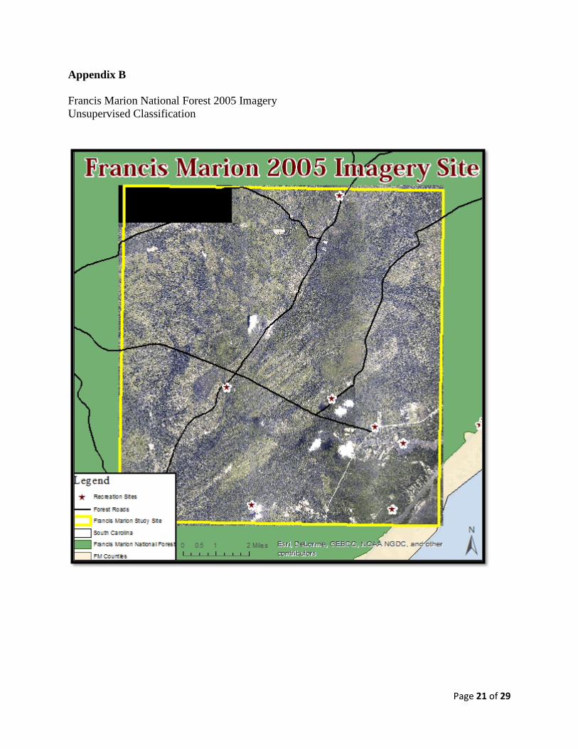
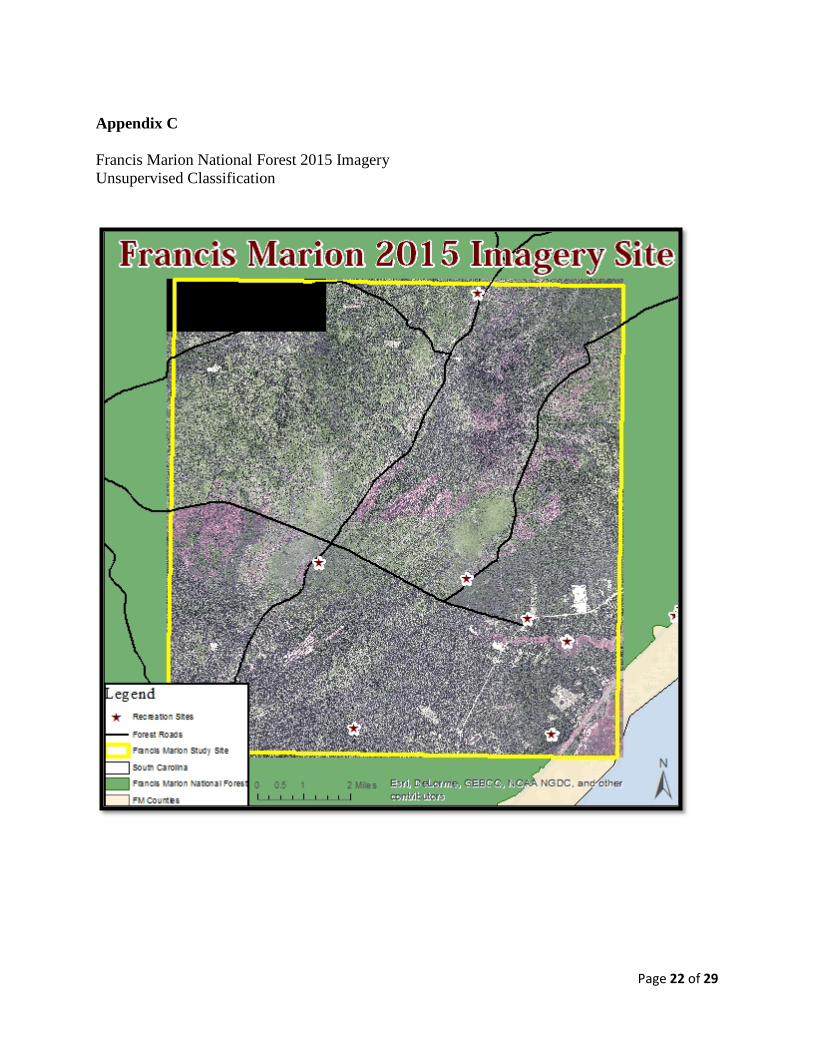
Change Detection Methods
The purpose of completing an unsupervised classification is to determine change between
two Landsat8 images. These changes are to confirm whether or not SLAMM can predict similar
changes with results that do not appear outside the realm of reason.
The images collected are already georeferenced, so the next step is to clip them according
to the study site. From there, each image undergoes the unsupervised classification process based
on 25 classes (just like SLAMM). This classification uses isodata clusters to better classify into
25 categories. From there each image is examined to highlight and identify the classifications,
and then recoded into 10 categories based on similarities. The matrix union of the two images
produces the changes of the amount of cells from 2005 to 2015. These values then are calculated
to show the percent difference between the two years. These differences are compared to the
SLAMM results to determine any similarities or differences.
Note: There will be differences due to the differences in categories that SLAMM
provides, with its main focus on various wetlands type. As a novice in remote sensing, I am
learning the best ways to determine the differences in land cover types, including the various
wetlands and marshes.
Results
The model produces various outputs. For my project, I selected the results to be displayed
as rasters, gifs, and tabular data. The images show some change within the SLAMM color codes;
Page 16 of 29
however, it is the number of cells for each category and their changes from previous years that
supplies us with sea level rise evidence.
The most important outcomes of these results, in my opinion, are focused on the following
categories: Estuarine Open Ocean, Tidal Flats, and Inland Fresh Marsh. These categories
determine some of the most important consequences of increased sea level rise.
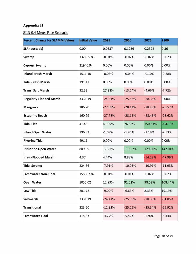
• The increase of Estuarine Open Ocean by 142% in the 0.4 Meter Scenario, 161.19 %
in the A1B Scenario, 208.3% in the 3.0 SLAMM 0.4 Meter Version and even 81.39% in
the imagery analysis proves that there will be more ocean water and it will be impeding
on the previous areas of marsh land.
• The Tidal Flats show an increase in all three scenarios and in the image analysis, leading
to the conclusion of more salt water coming in from the tides creating larger tidal flats.
Tidal Flats: 204.13% in the 0.4 Meter Scenario, 199.45 % in the A1B Scenario, 76.99%
in the 3.0 SLAMM 0.4 Meter Version and even 18.29% in the imagery.
• The Inland Fresh Marsh show a decrease or no change at all in the three scenarios and a
decrease in the image analysis, predicting less fresh marshes within the study site. This
potentially could cause coastal droughts, however, it could also imply more fresh marshes
moved inland, outside of the study site. Inland Fresh Marsh: -0.28% in the 0.4 Meter
Scenario, -1.24% in the A1B Scenario, and 0.00% in the 3.0 SLAMM 0.4 Meter
Version.
As a novice imagery analyst, my classification of land cover categories did not match up to
the exact SLAMM codes. However, the most important values are noted: an increase in water by
81.39% and a decrease in wetlands of 39.32%. These values prove that SLR will be affecting the
Francis Marion Forest and that preventative measures need to be included within the Forest Plan.
Page 17 of 29
Obstacles, Benefits, & Limitations
Running an unfamiliar model takes time to understand the processes and procedures.
Overall, SLAMM is an extremely useful tool that provides value outputs. The major obstacles
would be gathering data and matching their cell extent to one another exactly. Without GIS
experience, running this model would prove very difficult, in particular, converting the data to
the appropriate formats and matching their cell size would be daunting.
Benefits
• SLAMM provides extensive looks at the changes in all wetlands types
• Predicts the changes within your specific parameter request
• Allows for various climate scenarios to be explored
• Understanding potential increases in sea level rise will allow for better preparation for
recreation sites as well as transportation
• Once the areas of interest are located, ecologists or biologists can determine the
species in those areas that may need protection
• SLAMM provides tabular results, GIS outputs, gif formats, rasters for every
parameter provided
Limitations
SLAMM
• Higher Resolution = slower run time
• ASCII Binary files require extensive storage
• A lot of inputs can be difficult to access and hard to convert for the average
GIS user
Imagery analysis
• Imagery requires an expert eye
• High Resolution leads to difficult classification
o Example: Clouds = Driveways
• Various colors of wetlands make for difficult classification: low tide or high
tide, sand influx, recent storm effects, etc.
Page 18 of 29
Conclusions
The Sea Level Affecting Marshes Model is a valuable tool for coastal management. This
program will comprehend what type of marshes or wetlands will be affected and by how much.
The percent change between each year provides the user with a better understanding for each
time step. Coupled with the image processing and the SLAMM 3.0 version outputs, it is clear
that even those the values are not identical, the results are within a reasonable range from one
another. The model produced appropriate results to which the Forest Plan can use to create
restoration and preventive policies. The next step in this project would be to incorporate
biological or ecological data sets. These datasets were difficult to acquire during this timeframe,
however coupling the species data and the areas of potential flooding and habitat changes, the
prediction of future species effects are possible. Not only species impacts, but a decrease in fresh
water and an increase in salt marshes will rate high on the coastal drought possibility, finding
that data and incorporating it will allow for understanding of potential fire locations. Coastal
drought can dry out flammable marshland soils, leading to possible long burning peat fires.
Increases in tidal flooding can cause salinity stress on species rich coastal forests. A nearby
county, Georgetown, has saltwater intrusion issues, which SLR can exacerbate; using the results
from the model will allow for when and where the SLR can affect the drinking water within the
National Forest and how to prepare for it. From there the Forest Plan can determine the best
plans of action to arrange for the future, every only ten years at a time if interested.
The Francis Marion Forest Plan specifically wanted to understand how sea level rise is
influencing the ecosystems and how to create related management. These results show where the
sea level rise will affect and how the environments will change. The next step is to collaborate
with species knowledgeable people in those impacted areas. They will have much better opinions
than my own to understand how to start preparing for these changing habitats.
Page 19 of 29
Bibliography I. Rodríguez ⁎, I. M. (2007). Geographic Information Systems applied to Integrated Coastal Zone
Management. Geomorphology, 100-105.
IPCC. (2016, July). International Panel on Climate Change. Retrieved from The IPCC Special Report on Emissions Scenarios (SRES): https://www.ipcc.ch/ipccreports/tar/wg1/029.htm#storya1
Kirsten Lackstrom, A. B. (2015). Drought and Coastal Ecosystems: An Assessment of Decision Maker Needs for Information. Charleston, SC: Carolinas Integrated Sciences & Assessments, University of South Carolina.
Naughton, M. P. (2013). SLAMM (SEA LEVEL AFFECTING MARSHES MODEL) Modeling of the Effects of SLR on Coastal Wetland Habitats of San Diego County. San Diego: San Diego State University.
Nieves, D. P. (2009). Application of the Sea-Level Affecting Marshes Model (SLAMM 5.0.2) in the Lower Delmarva Peninsula. Arlington, VA: Conservation Biology Program National Wildlife Refuge System.
Patty Glick, J. C. (2008). Sea-Level Rise and Coastal Habitats in the Chesapeake Bay Region. Eastern Shore, VA: National Wildlife Federation.
Polaczyk, D. A. (2013, October 22). The Sea Level Affecting Marshes Model (SLAMM). Retrieved from Warren Pinnacle Consulting, Inc.: http://www.gulfmex.org/wp-content/uploads/2014/01/SLAMM_Oct-22_am_presentation_web.pdf
Service, U. F. (2016). Francis Marion NF 2016 Forest Plan Draft. Charleston: USDA.
USDA. (2016). US Forest Service Francis Marion National Forest. Retrieved from Francis Marion and Sumter National Forests : http://www.fs.usda.gov/detail/scnfs/home/?cid=fsbdev3_037393
USGS. (2014). USGS Real-Time Salinity Drought Index. Charleston, SC: Coastal Drought Monitoring Knowledge Assessment WorkshopUSGS.
Warren Pinnacle Consulting, Inc. (2012). SLAMM 6.3 Technical Documentation. Warren Pinnacle Consulting, Inc.
Page 20 of 29
Appendix A Francis Marion National Forest Map
Page 21 of 29
Appendix B Francis Marion National Forest 2005 Imagery Unsupervised Classification
Page 22 of 29
Appendix C Francis Marion National Forest 2015 Imagery Unsupervised Classification

Page 23 of 29
Appendix D SLAMM Interface 1.
SLAMM Interface 2.
Page 24 of 29
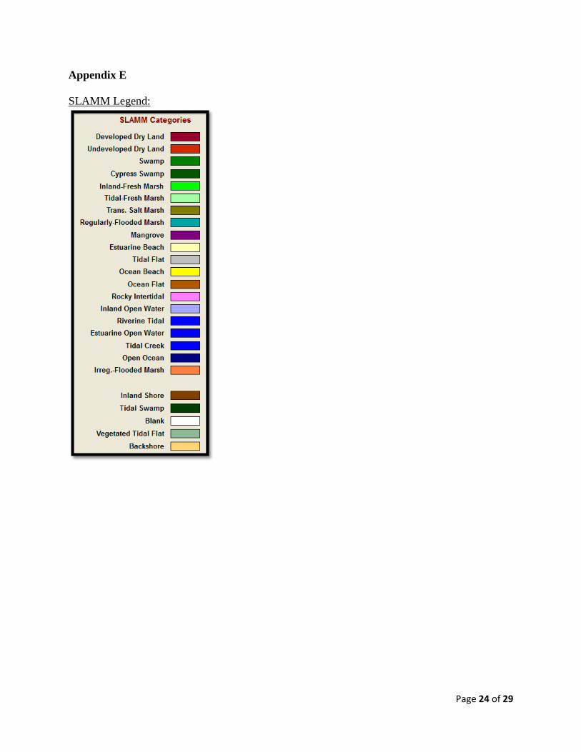
Appendix E SLAMM Legend:
Page 25 of 29
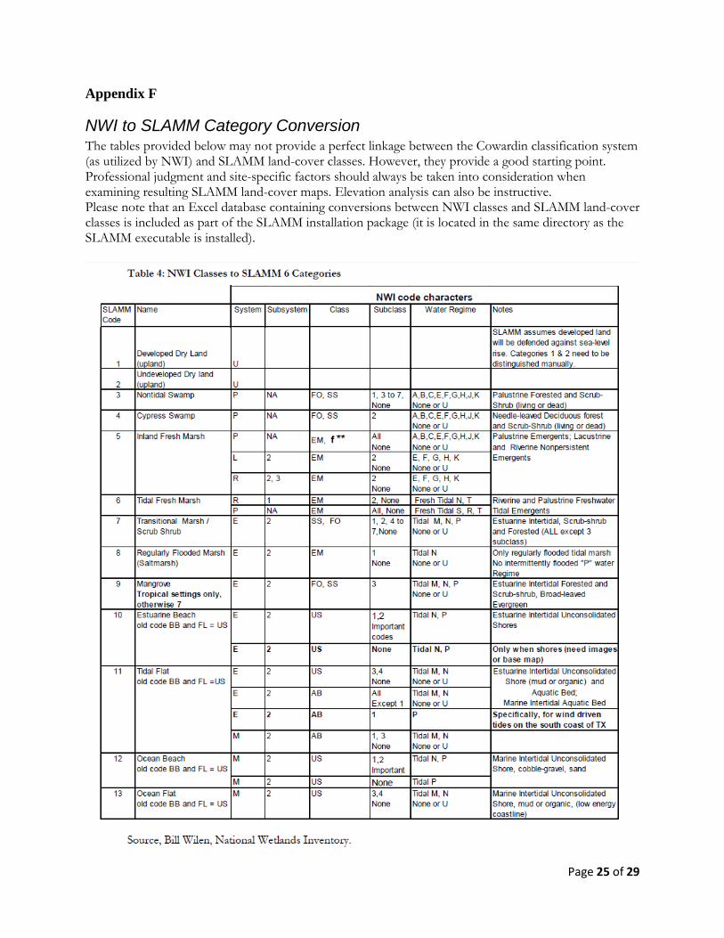
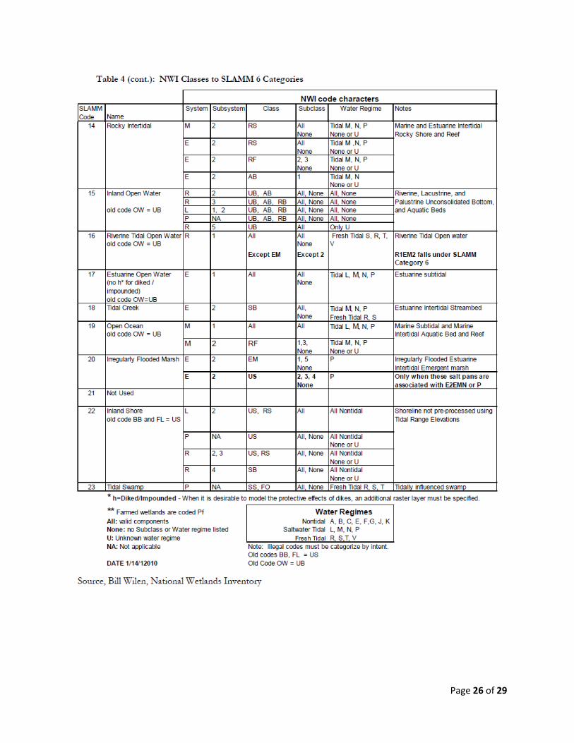
Appendix F
NWI to SLAMM Category Conversion The tables provided below may not provide a perfect linkage between the Cowardin classification system (as utilized by NWI) and SLAMM land-cover classes. However, they provide a good starting point. Professional judgment and site-specific factors should always be taken into consideration when examining resulting SLAMM land-cover maps. Elevation analysis can also be instructive. Please note that an Excel database containing conversions between NWI classes and SLAMM land-cover classes is included as part of the SLAMM installation package (it is located in the same directory as the SLAMM executable is installed).
Page 26 of 29
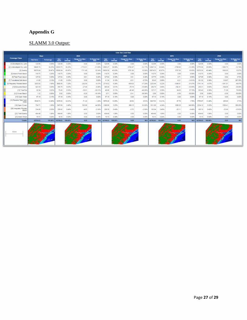
Page 27 of 29
Appendix G SLAMM 3.0 Output:
Page 28 of 29
Appendix H
SLR 0.4 Meter Rise Scenario
Percent Change for SLAMM Values Initial Value 2025 2050 2075 2100
SLR (eustatic) 0.00 0.0337 0.1236 0.2392 0.36
Swamp 132155.83 -0.01% -0.02% -0.02% -0.02%
Cypress Swamp 21940.94 0.00% 0.00% 0.00% 0.00%
Inland-Fresh Marsh 1511.10 -0.03% -0.04% -0.10% -0.28%
Tidal-Fresh Marsh 191.17 0.00% 0.00% 0.00% 0.00%
Trans. Salt Marsh 32.53 27.88% -13.24% -4.66% -7.72%
Regularly-Flooded Marsh 3331.19 -24.41% -25.53% -28.36% 0.00%
Mangrove 186.70 -27.39% -28.14% -28.26% -28.57%
Estuarine Beach 160.29 -27.78% -28.15% -28.45% -28.62%
Tidal Flat 41.43 41.95% 76.65% 150.61% 204.13%
Inland Open Water 196.82 -1.09% -1.40% -2.19% -2.53%
Riverine Tidal 49.11 0.00% 0.00% 0.00% 0.00%
Estuarine Open Water 809.09 17.21% 119.67% 129.00% 142.01%
Irreg.-Flooded Marsh 4.37 4.44% 8.88% -54.22% -47.99%
Tidal Swamp 224.66 -7.91% -10.03% -10.91% -11.93%
Freshwater Non-Tidal 155607.87 -0.01% -0.01% -0.02% -0.02%
Open Water 1055.02 12.99% 91.52% 98.52% 108.44%
Low Tidal 201.72 -9.02% -6.63% 8.33% 19.19%
Saltmarsh 3331.19 -24.41% -25.53% -28.36% -31.85%
Transitional 223.60 -12.82% -25.25% -25.34% -25.92%
Freshwater Tidal 415.83 -4.27% -5.42% -5.90% -6.44%
Page 29 of 29
Appendix I
SLR A1B Scenario
Percent Change for SLAMM Values
(A1B Scenario ~0.6 Meter Rise) Initial Value 2025 2050 2075 2100
SLR (eustatic) 0.00 0.0337 0.1236 0.2392 0.36
Swamp 132155.83 -0.01% -0.02% -0.02% -0.05%
Cypress Swamp 21940.94 0.00% 0.00% 0.00% 0.00%
Inland-Fresh Marsh 1511.10 -0.03% -0.06% -0.29% -1.24%
Tidal-Fresh Marsh 191.17 0.00% 0.00% 0.00% 0.00%
Trans. Salt Marsh 32.53 42.45% -5.63% 6.09% 58.53%
Regularly-Flooded Marsh 3331.19 -25.07% -26.20% -31.96% -71.34%
Mangrove 186.70 -27.72% -28.23% -28.58% -28.60%
Estuarine Beach 160.29 -27.86% -28.28% -28.65% -47.44%
Tidal Flat 41.43 51.45% 102.89% 151.17% 199.45%
Inland Open Water 196.82 -1.11% -1.83% -2.45% -2.65%
Riverine Tidal 49.11 0.00% 0.00% 0.00% 0.00%
Estuarine Open Water 809.09 12.19% 121.52% 132.22% 161.19%
Irreg.-Flooded Marsh 4.37 4.44% -32.78% -32.78% -33.53%
Tidal Swamp 224.66 -8.55% -10.59% -11.95% -27.10%
Freshwater Non-Tidal 155607.87 -0.01% -0.02% -0.02% -0.05%
Open Water 1055.02 9.14% 92.85% 100.94% 123.12%
Low Tidal 201.72 -0.67% -1.34% 57.75% 195.00%
Saltmarsh 3331.19 -25.07% -26.20% -31.96% -71.34%
Transitional 223.60 -8.38% -24.30% -23.56% -2.10%
Freshwater Tidal 415.83 -4.62% -5.72% -6.46% -14.64%