PHYSICAL REVIEW E 87, 023010 (2013)

Reactive transport in porous media: Pore-network model approach compared to pore-scale model

Clement Varloteaux,1,* Minh Tan Vu,2 Samir Bekri,1,† and Pierre M. Adler2,‡1IFP Energies nouvelles, 1 et 4 avenue de Bois-Preau, 92852 Rueil-Malmaison, France

2Sisyphe, UPMC, 4 place Jussieu, 75252 Paris, France(Received 1 October 2012; published 15 February 2013)

Accurate determination of three macroscopic parameters governing reactive transport in porous media, namely,the apparent solute velocity, the dispersion, and the apparent reaction rate, is of key importance for predictingsolute migration through reservoir aquifers. Two methods are proposed to calculate these parameters as functionsof the Peclet and the Peclet-Dahmkohler numbers. In the first method called the pore-scale model (PSM), theporous medium is discretized by the level set method; the Stokes and convection-diffusion equations with reactionat the wall are solved by a finite-difference scheme. In the second method, called the pore-network model (PNM),the void space of the porous medium is represented by an idealized geometry of pore bodies joined by porethroats; the flow field is computed by solving Kirchhoff’s laws and transport calculations are performed in theasymptotic regime where the solute concentration undergoes an exponential evolution with time. Two syntheticgeometries of porous media are addressed by using both numerical codes. The first geometry is constructed inorder to validate the hypotheses implemented in PNM. PSM is also used for a better understanding of the variousreaction patterns observed in the asymptotic regime. Despite the PNM approximations, a very good agreementbetween the models is obtained, which shows that PNM is an accurate description of reactive transport. PNM,which can address much larger pore volumes than PSM, is used to evaluate the influence of the concentrationdistribution on macroscopic properties of a large irregular network reconstructed from microtomography images.The role of the dimensionless numbers and of the location and size of the largest pore bodies is highlighted.

DOI: 10.1103/PhysRevE.87.023010 PACS number(s): 47.56.+r, 47.11.−j, 47.15.G−

I. INTRODUCTION

When a reactive fluid is injected into a porous medium,chemical reactions can modify the petrophysical properties ofthe porous media, such as the porosity ε and the permeabilityK . This physical phenomenon consists of two coupled majorprocesses, namely, solute transport and reaction at the fluid-solid interface, which depend on the initial conditions, onthe geometry, and also on the nature of the components. Animportant application of such studies is carbon dioxide storagein saline aquifers where dissolution of CO2 in brine may causeits acidification and thus mineral dissolution [1,2].

The main objective of this paper is to determine thedistribution of the solute by two different numerical methodsand to compare the results.

In the pore-scale model (PSM) developed by Bekri et al.[3], the porous medium is represented by void and solidvoxels (voxel method). Local equations governing the soluteconcentration are solved by the finite-difference method. Then,the evolution of rock-fluid interfaces is calculated and theporosity and permeability modifications are determined. Inorder to accurately simulate the complex surface motions, thevoxel method is replaced by the level set method (LSM) [4].The advantage of the LSM is that it can deal with curvesand surfaces on a fixed Cartesian grid without having toparametrize these objects. Also, the LSM can follow shapesthat change topology, for instance, when it splits into two or,reversely, develops holes [5].

*clement.varloteaux@ifpen.fr†samir.bekri@ifpen.fr‡pierre.adler@upmc.fr

The PSM combined with the LSM is an accurate method,but it is time consuming and only limited pore volumescan be addressed. An alternative method is the pore-networkmodel (PNM) which allows one to study reactive transportphenomena in much larger pore volumes with the same com-putational resources. This approach is based on a simplifiedmicrostructure of the porous medium, which is schematizedby pore bodies connected by pore throats [6–11].

The PNM is versatile and can account for various phenom-ena occurring on the pore scale. It was originally developedby Fatt [12] to calculate multiphase flow properties of porousmedia. Over the last decades, it has been extensively used tosimulate basic phenomena such as capillarity and multiphaseflow through porous media [8,13–16]. This approach wasextended to study pore evolution and changes in petrophysicalproperties due to particle capture [17], asphalt precipitation[18], deposition and dissolution in diatomite [19], and fil-tration combustion [20]. Recently, adsorption and reactionprocesses were tentatively integrated into the PNM. Raoofet al. [21] quantified the effective kinetics of adsorptionprocesses whereas Li et al. [22] and Kim [23] concentratedtheir research on effective reaction rates in porous media usingthe PNM and its possible implementation on the reservoirscale. Algive et al. [24,25] proposed the PNM approach tostudy mineral dissolution and precipitation caused by CO2

sequestration.In this paper, the PSM is used to validate the PNM for reac-

tive transport phenomena since unexpected phenomena wereobserved in the PNM at the beginning of this work. Sections IIand III describe the PSM and the PNM, respectively. In Sec. IV,the two models are compared on synthetic cases. Then, PNMhypotheses are validated and the accuracy of the model isassessed by PSM calculations; various reaction regimes whichoccur in a case study are illustrated and explained. Section V

023010-11539-3755/2013/87(2)/023010(15) ©2013 American Physical Society

VARLOTEAUX, VU, BEKRI, AND ADLER PHYSICAL REVIEW E 87, 023010 (2013)

is devoted to the application of the PNM to a large irregularnetwork derived from microtomography measurements.

II. PORE-SCALE MODEL

The pore-scale model is based on the resolution of theStokes equation and of the convection-diffusion equationsupplemented by conditions on the deposition or dissolutionflux at the walls. These equations are discretized by a finite-difference scheme which is detailed by Bekri et al. [3].

The LSM is used to smooth out the fluid-rock interfaces.The most important improvement provided by the LSM is thatthe boundary conditions are written at the level set surface andnot at the discretized surface by voxels. Furthermore, the fluxat the interface is precisely computed by using the unit vectorwhich is normal to the smooth surface.

A. Governing equations

Consider reactive transport in a porous medium � whichconsists of a fluid phase �F and a solid phase �S separated byan interface �.

When the flow is steady and when inertial effects arenegligible, the fluid motion is governed by the Stokes equation.Hence,

μ∇2v + ∇p = 0 in �F , (1a)

∇ · v = 0 in �F , (1b)

where μ is the viscosity of the fluid, which is assumed to beconstant, p is the pressure, and v is the fluid velocity.

The no-slip condition should be satisfied at the fluid-solidinterface �:

v = 0 on �. (1c)

The solute flux J can be written as

J = cv − D∇c, (2a)

where D is the solute molecular diffusion and c is the soluteconcentration. D is assumed to be constant.

When there is no bulk chemical reaction, c obeys the localconvection-diffusion equation

∂c

∂t+ ∇ · (cv − D∇c) = 0 in �F . (2b)

The boundary condition for c at the wall � is assumed tobe a first-order surface reaction:

n · J = κ(c − c) on �, (2c)

where κ is the local reaction rate constant and c is theequilibrium concentration of the solute.

This reaction causes a displacement W normal to the wall,which is proportional to the solute flux at the wall [3],

∂W

∂t= −KcρF κ(c − c) on �, (3)

where ρF is the fluid density and Kc is the stoichiometriccoefficient of the reaction. Of course, the velocity of thisdisplacement is assumed to be very small with respect to thefluid velocity.

B. Dimensionless formulation

In order to derive the parameters which control the problem,the previous equations can be made dimensionless by intro-ducing a characteristic length scale lc for the porous mediumand a characteristic velocity chosen as the interstitial velocity〈v〉. Similarly, the average concentration 〈c〉 is defined as theconcentration scale. Thus, a new system of dimensionlessvariables indicated by primes can be defined:

∇′ = lc∇, v′ = v〈v〉 , p′ = plc

μ〈v〉 , c′ = c − c

〈c〉 − c,

(4)

t ′ = t

Twith T = l2

c

KcρD(〈c〉 − c).

The dimensionless equations are

∇′2v′ − ∇′p′ = 0 in �F , (5a)

∇′ · v′ = 0 in �F , (5b)

v′ = 0 on �, (5c)

Pe∇′c′ · v′ − ∇′2c′ = − L2

DT

∂c′

∂tin �F , (5d)

n · ∇′c′ = −PeDa c′ on �, (5e)∂W ′

∂t ′= PeDa c′ on �, (5f)

where the dimensionless Peclet and Dahmkohler numbers aredefined as

Pe = 〈v〉lcD

, Da = κ

〈v〉 . (6)

Pe compares convection and diffusion while Da comparesthe speed of the chemical reaction and the fluid velocity. Theproduct of these two numbers, PeDa, is often used; it comparesreaction to diffusion characteristic times.

In addition, the system is assumed to be not very far fromchemical equilibrium and that the rate of deformation of thesolid surface is very slow; hence, the velocity field in thefluid can be determined at any time by solving (5a)–(5c). For agiven geometry and velocity field, the dimensionless equationsgoverning c′ possess a solution of the form e−γ t c′(x′). We shallassume that the time required to reach the asymptotic regimeis small compared to the wall evolution characteristic time.Consequently, the geometrical changes mainly occur duringthe asymptotic regime and the asymptotic concentration fieldis used to determine the wall evolution rate.

C. Level set method

The solid-liquid interface is tracked by means of the LSM.In this method, the real surface is defined by a distancefunction based on the usual fixed Cartesian grid. The interfaceis represented by a triangulated surface at the zero level ofthis distance function. The numerical codes using this methodsolve transport and flow fields more accurately and topologychanges are effectively handled [5].

The LSM represents the interface �(x) as the zero-levelcontour of a function φ(x,t) [26]:

� = {x|φ(x,t) = 0}. (7)

023010-2

REACTIVE TRANSPORT IN POROUS MEDIA: PORE- . . . PHYSICAL REVIEW E 87, 023010 (2013)

Moreover, the level set function φ(x,t) satisfies the propertiesthat φ > 0 for phase 1 and φ < 0 for phase 2. In practice,φ(x,t) is a signed distance function.

The chain derivation rule applied to φ(x,t) yields

∂φ

∂t+ ∇φ · dx′

dt= 0. (8)

Let n be the normal to � pointing outward of the solidphase:

n = ∇φ

‖∇φ‖ . (9)

The velocity of the interface is defined along n as

Vi = dx′

dt· n. (10)

This propagation velocity Vi is related to (5f) by

Vi = ∂W ′

∂t ′= PeDa c′ on �. (11)

Finally, the evolution of the level set function φ isgoverned by

∂φ

∂t+ Vi‖∇φ‖ = 0 (12)

for a given initial geometry φ(x,t = 0).

D. Algorithm description

During the simulation, the coupled Stokes (5a) andconvection-diffusion (5d) equations are solved by the samealgorithm as used by Bekri et al. [3] which comprises fivesteps. (i) The velocity field vn and the concentration field cn arecalculated for the current interface φn. (ii) The concentrationat the interface is extrapolated from the field cn to calculate theinterface propagation velocity F (11). (iii) The new interfaceφn+1 is determined at time tn+1 by using the interface velocityand (12). (iv) The new interface is updated and the medium isvisualized. (v) This process is repeated until the end conditionis verified.

This algorithm is schematized in Fig. 1.

III. PORE-NETWORK MODEL

The PNM describes the flow and the transport on the porescale. It can address larger pore volumes than can the PSM withthe same computational resources. This section describes theporous medium representation and the resolution of flow andconcentration in the asymptotic regime defined in Sec. II B;therefore, only long-term phenomena are studied.

A. Geometry

The PNM is based on a simplified representation of the voidspace, which is approximated by a network of bonds (porethroats) and nodes (pore bodies) with an idealized geometry;the pore bodies are spherical while the pore throats arecylindrical channels with a circular, square, or triangular crosssection. The distinction between pore bodies and pore throatsand their simplified geometry makes complex problems easierto solve by using analytical or semianalytical solutions [27].

FIG. 1. General scheme of the reactive transport resolution by thePSM combined with the LSM.

The pore network can be a regular or an irregular three-dimensional lattice structure (Fig. 2). In Fig. 2(a), the porespace is defined on a cubic lattice where each pore bodyis assumed to be connected to six pore throats; therefore,the coordination number is equal to 6. The ratio betweenthe pore-body and the pore-throat diameters (aspect ratio) isconstant. The pore-throat diameters are randomly generatedaccording to a given probability density function. Of course,the coordination number and the aspect ratio can be variable.

In order to construct a representative pore network of aporous medium, the probability density function has to bechosen in order to reproduce some petrophysical parameters

FIG. 2. Pore-network models (a) reconstructed with a reg-ular lattice in order to reproduce petrophysical properties ofreal porous media [28] and (b) extracted from microtomographymeasurements [29].

023010-3

VARLOTEAUX, VU, BEKRI, AND ADLER PHYSICAL REVIEW E 87, 023010 (2013)

such as porosity and permeability. In addition, Bekri andVizika [28] recommend that the formation factor and thecapillary pressure curve be equal to those of the consideredporous medium since they are very sensitive to its structure.The choice of a compatible pore-throat size distribution is akey parameter for the construction of a representative porenetwork using this cubic structure.

An alternative to the regular lattice pore network has beenrecently developed in order to get closer to the real mediumgeometry [7,29–31]. This method made important progressbecause of synchrotron computed microtomography, whichgenerates three-dimensional (3D) data sets on the micrometerscale.

The first step of this method is to measure the exact 3D porespace of the porous medium. Then, a 3D image in gray levelsis reconstructed using x-ray microtomography. A thresholdis chosen to distinguish between pores and rock. Then, theskeleton of the pore space is computed by a hybrid algorithmwhich combines thinning and a distance map such as the onederived by Thovert et al. [32]. Additionally, the pore space ispartitioned into pore bodies and pore throats according to theconceptual description of the pore-network model [Fig. 2(b)].Finally, geometrical parameters are extracted from the 3Dpore-space images [see [29], for more details].

B. Flow field

The fluid flow is governed by the Stokes equations (1). Thefluid velocity in the capillary tubes which compose the porenetwork is given by the Poiseuille parabolic profile

v(ρ) = 2vz

(1 − ρ2

r2

)z with vz = − r2

8μ

∂P

∂z, (13)

where r and ρ are the radius of the tube and the radialcoordinate, respectively, and z is the unit vector parallel tothe tube axis. The pressure drop between two neighbor porebodies, P , is related to the flow rate Q passing through thecapillary tube by

Q = vzS = πr4

8μ

P

Lz

, (14)

where Lz is the length of the capillary tube.The pore-body flow field is conceptually more difficult

to define analytically. For the sake of simplicity, pressure isassumed to be constant within a pore body; in other words,the velocity in pore bodies is assumed to be zero and thereforenegligible compared to the velocity in the pore throats.

Then, a mass balance is performed over each pore body anda linear system for the pressures can be derived,

G · P = b, (15)

where G is the conductivity matrix, which only depends on thegeometric properties of the network, P is the unknown pressurevector, and b is a vector related to the external boundaryconditions.

By using a linear solver such as a conjugate gradienttechnique [33], the entire pressure field can be evaluated foran imposed pressure drop over the network. Thus, Eqs. (13)provide velocity in every pore throat.

When the pressure and velocity fields are known, thepermeability K of the porous medium can be computed as

K = Qtot

Stot

μLtot

P, (16)

where Qtot is the total flow rate passing through the crosssection Stot of the porous medium; Ltot and P are the totallength and the pressure drop over the network.

C. Concentration field

A comparable approach to flow is used to compute the con-centration field within a pore network. An analytical solutionof the local problem is provided for the simplified geometryused in the PNM. The flux at the pore body–pore throatinterface and the concentration are related by an analyticalsolution. Mass balance yields a nonlinear system solved byan optimization algorithm which provides the concentrationdistribution within the pore network. This section presents theanalytical solutions for the pore bodies and the pore throats.Then, the concentration field within the whole pore network isdetermined.

1. Pore throats

The resolution of the reactive transport in a pore throat isdivided into two steps. First, the transverse profile is calculatedby assuming that the flow and transport transverse profiles areestablished. Second, a macroscopic equation governing theaverage concentration in the cross section is deduced.

The reactive transport within simple geometries such asparallel plates, infinite tubes, or closed spheres has alreadybeen studied [24,34,35]. For example, Bekri et al. [3] providethe analytical solution between two infinite parallel plates.

As explained at the end of Sec. II B, the system is assumed tobe close to chemical equilibrium and the rate of deformation ofthe surface is assumed to be very slow; the transitional regimeis short compared to the asymptotic regime and the asymptoticregime is assumed to be reached. For a first-order reaction,this assumption is equivalent to supposing that the normalizedconcentration c′ (4) undergoes an exponential decay with timecharacterized by the decrease rate λ:

c′(ρ,t) ≈ X(ρ) exp(−λt), (17)

where X is the transverse profile of c′.For an infinite cylinder, X can be written as a function of

the Bessel functions J0 and J1:

X(ρ ′) = ω2

2PeDa

J0(ωρ ′)J0(ω)

Xt (18a)

with Xt = 1

S

∫S

Xd2s, (18b)

where ρ ′ is the dimensionless radial coordinate (ρ ′ = ρ/r). ω

is the first positive solution of the equation

ωJ1(ω)/J0(ω) = PeDa. (19)

Calculation details are provided in Appendix A 1.

023010-4

REACTIVE TRANSPORT IN POROUS MEDIA: PORE- . . . PHYSICAL REVIEW E 87, 023010 (2013)

Using (18a), Shapiro and Brenner [35] showed that theaverage normalized concentration c′(z) is governed by

∂c′

∂t+ ∂

∂z

(v∗c′ − D∗ ∂c′

∂z

)+ γ ∗c′ = 0 (20a)

with c′ = 1

S

∫S

c′d2s, (20b)

where γ ∗, v∗, and D∗ are the apparent volume reaction rate, theapparent velocity, and the dispersion of the solute, respectively.These coefficients, which characterize the solute behaviorin the pore throats, can be derived from the spatial globalmoments mi of the concentration [36]:

γ ∗ = − 1

m0

d

dt(m0), (21a)

v∗ = d

dt

(m1

m0

), (21b)

D∗ = 1

2

d

dt

[m2

m0−

(m1

m0

)2], (21c)

with mi(t) =∫

c(r,t)rid3r, (21d)

where r is the spatial position within the pore throat.Furthermore, for capillary tubes, Algive et al. [25] provided

analytical expressions of γ ∗, v∗, and D∗ as functions of Peand PeDa. These functions are deduced from a numericalapplication of the formulation of Sankarasubramanian andGill [34] and from the propagation of a particle cloudusing a random-walk technique. Thanks to these formulas,macroscopic coefficients can be assigned to each pore throatand pore body of the pore network.

Moreover, since only long-term phenomena are studied,the asymptotic regime can be generalized to the whole porenetwork. Thus, a unique exponential decrease rate is definedwhich is common to every element of the pore network. Let ϒ

be this decrease rate. Then c′ in a pore throat can be written as

c′(z,t) = Xt (z) exp(−ϒt). (22)

Introduction of (22) into (20a) yields a second-order ordinarydifferential equation

∂2Xt

∂z′2 − Pet ∂Xt

∂z′ − PeDat Xt = 0(23)

with Pet = v∗lD∗ and PeDat = (γ ∗ − ϒ)l2

D∗ ,

where l is the length of the pore throat and z′ = z/l is thedimensionless longitudinal coordinate along the tube. Thedistribution of the solute within pore throats can be deducedeasily from this second-order ordinary differential equationas a function of Xt at the edges of the pore throat, denotedXt (z′ = 0) and Xt (z′ = 1) (cf. Fig. 3).

2. Pore bodies

The reasoning applied to the resolution of the concentrationdistribution within pore throats cannot be generalized to porebodies where the velocity is not calculated. Hence, X(ρ ′) inpore bodies is limited to only two forms based on dominantdiffusion or perfect mixing.

FIG. 3. Schematization of a pore throat connecting the two porebodies i and Iij .

Perfect mixing implies a uniform c′ in the pore body. Fordominant diffusion, c′ in a sphere of radius R is controlled bydiffusion and reaction; therefore,

X(ρ ′) = ω2

3PeDa

sin(ωρ ′)ρ sin(ω)

X (24a)

with X = 1

V

∫V

Xd3x, (24b)

where ρ ′ = ρ/R is the dimensionless radial coordinate. ω isthe first positive solution of

1 − ω

tan ω= PeDa. (25)

The flux at ρ ′ = 1 is given by

�w =(

1 − ω

tan ω

)ω2

3PeDaX. (26)

Details of the calculations are provided in Appendix A 2.

3. Pore network

Then, the mass balance over each pore body i of the networkyields

PeDap

i Xi =ni∑

j=1

�ij with PeDap = (γ ∗ − ϒ)R2

D∗ , (27)

where the subscripts i and j correspond to the ith and j th porebodies; �ij are the solute fluxes at the interface between thenj connected neighbor pore throats (with nj also called thecoordination number) and the ith pore body. The left side of(27) is the sink-source term of the reaction in the pore body.�ij is derived from the analytical solution of (23):

� =[

− ∂Xt

∂z′

∣∣∣∣z′=0

+ Pet Xt (0)

]= ϕXt (0) + ψXt (1), (28)

where ϕ and ψ are coefficients derived from the resolutionof (23).

The neighbor pore body connected through pore throat j

to the ith pore body is denoted by Iij (cf. Fig. 3). Using thisnotation, the end conditions of a pore throat become

Xt (z′ = 0) = ξiXi and Xt (z′ = 1) = ξIijXIij

, (29)

where ξ is equal to 1 when perfect mixing is assumed or equalto ω2

3PeDa for dominant diffusion [ρ ′ = 1 in (24a)].Thus, the mass balance (27) becomes

PeDap

i Xi =nci∑j=1

(ϕij ξiXi + ψij ξIij

XIij

). (30)

023010-5

VARLOTEAUX, VU, BEKRI, AND ADLER PHYSICAL REVIEW E 87, 023010 (2013)

N equations (where N is the number of pore bodies inthe network) with N + 1 unknowns can be written for themass balance of each pore body. Indeed, the unknowns areXi=1,...,N for each pore body, to which should be added theoverall decrease rate of the normalized concentration ϒ (22).Thus, a closure equation is needed and it is provided by thenormalization of the dimensionless concentration (4).

Moreover, because ϕij and ψij are related to ϒ throughPeDap, (30) involves some nonlinear terms which are productsof unknowns. Thus, the iterative Newton-Raphson method [33]is used to solve the resulting nonlinear system.

In the first iteration, perfect mixing is assumed in all thepore bodies. Then, during the iterative process, the solution ofdominant diffusion (24a) is assigned if all the fluxes �ij of agiven pore body, computed at the previous iteration, have thesame sign. At any iteration, when this minimal criterion is nolonger met, the pore body switches back to perfect mixing.Of course, the closer to (26) solute fluxes �ij are, the moreaccurate the dominant diffusion solution is.

D. Algorithm description

The evolution of the geometry due to reaction is computedthrough an iterative process based on porosity modificationsas detailed in Fig. 4. For a given initial pore network, theflow field is determined in step 1 for an arbitrary pressuredifference between inlet and outlet [8]. Then, the porosity andthe permeability of the pore network are calculated as wellas the mean interstitial velocity. In step 2, a linear correctionis applied to the pressure difference to adjust the velocityfield to the imposed Pe. As in Algive et al. [25], the pore-scale transport coefficients γ ∗, v∗, and D∗ defined in (20a) aredetermined for each pore body and each pore throat in step 3.

FIG. 4. General scheme of the reactive transport resolution byusing the PNM.

In step 4, (30) is solved over the whole network and it yieldsX. Then, in step 5, the evolution of the geometry is taken intoaccount with (5f). Due to the variations of c′, the reaction is notuniformly distributed within an element of the pore network.To be consistent with the PNM formalism, the wall evolutionis averaged over each element of the pore network in order tokeep the original shape of the element. The wall evolution isadjusted in order to obtain small and controlled evolution ofthe porosity. Since the geometry of the new pore network iscompatible with the PNM, steps 1 to 5 are iterated (step 6) onthe updated pore network.

At the end of the simulation, porosity-permeability curvesand the macroscopic coefficients γ ∗, v∗, and D∗ are calculated.

IV. MODEL COMPARISONS

In order to evaluate the accuracy of the reactive PNM,it is compared with the PSM and observations of Daccordet al. [37] at the end of the first iteration of the generalschemes schematized in Fig. 1 for the PSM and Fig. 4 forthe PNM. It should be noticed that the pore-throat surfacedisplacement deduced from solute flux at the wall (3) is takeninto account differently in the two models. In the PSM, thesurface displacement is calculated for each voxel, while inthe PNM the pore-throat diameter evolution is deduced fromthe average solute flux over each surface element. Thus, theevolution of the pore geometry by the PSM would not stayconsistent with PNM formalism for long times; it should benoticed that this paper is not focused on this geometricalevolution and only the flux at the wall of the network iscalculated.

Two samples are addressed by both numerical codes.The first sample is used to validate the analytical solutionsimplemented in the PNM. The second one, which containsonly six pores, has been designed in order to highlight andunderstand the various possible reaction patterns observedin the asymptotic regime. Moreover, thanks to this reducedgeometry, a new reaction regime has been found.

A. Validation of the PNM assumptions

Consider the cubic pore network of 4 × 4 × 4 spheresinterconnected by capillary tubes, which is displayed in Fig. 5;it is called PN1. Each pore body is connected to six other ones.The mean flow is parallel to one of the main directions of thecubic network.

The pore-body diameters are stochastically generated witha Weibull probability density function. Pore-throat diametersare related to the smallest neighbor pore body by a ratio equal to4 between pore-body and pore-throat diameters. The distancebetween pore bodies is equal to 100 μm along all directions.

The study of the c′ field is focused on the main flow path andon the secondary flow path which passes through the largestpore body. These two flow paths are crucial for the descriptionand understanding of the field c′ (see Fig. 5). Both flow pathsare in the plane y = 100 μm. The main flow path is the onewhose axis is z = 200 μm and the center of the largest porebody is at x = 300 μm and z = 300 μm.

023010-6

REACTIVE TRANSPORT IN POROUS MEDIA: PORE- . . . PHYSICAL REVIEW E 87, 023010 (2013)

FIG. 5. Pore network PN1.

1. Flow field validation

In order to minimize discrepancy between the fields c′, thecomputed flow fields by both models have to be compared.

The transverse velocity profile obtained in pore throats bythe PSM can be used to validate the Poiseuille profile used inthe PNM. It should be emphasized that the pore space is theone shown in Fig. 5 and discretized by the LSM. The velocityprofile of the shortest pore throat obtained by using the PSMis compared in Fig. 6(a) to the analytical solution (13) used inPNM. As shown in Fig. 6(b), a good agreement is observedfor the mean velocity between two pore-body centers, despitethe hydraulic resistance of the pore bodies, which is not takeninto account in PNM.

The reactive transport solutions in this network are cal-culated with local values of Pe and PeDa. For the sakeof simplicity, the mean diameter of the network elements,lc = 〈d〉 = 18.98 μm, is chosen as the characteristic length.The molecular diffusion coefficient D is supposed to beconstant and equal to 10−9 m2 s−1. When the same Pe isimposed on both models, a comparable local velocity fieldis obtained, as observed in Fig. 6(c).

2. Concentration field validation

The normalized concentration obtained by the PSM in thepore space displayed in Fig. 5 and discretized by the LSMis used to validate the hypotheses implemented in the PNM;along a pore throat, X follows the analytical solution (18a)and does not depend on the longitudinal position; i.e., there isno effect of the boundaries of the pore throats. Figure 7 showsthe PSM X in one pore throat for PeDa = 1 and Pe = 1. Errorbars in Fig. 7 represent the spreading along the pore-throataxis of the values of X for the same radius. The PSM confirmsthat X can be considered as established along the pore throatsand follows the analytical solution (18a).

In Fig. 7, X is normalized by c′ in the pore-throat crosssection. However, c′ in PSM calculations depends on thelongitudinal position in the pore throat. It matches the solutionof the average equation (20a), which appears to be a good

(a)

(b)

(c)

FIG. 6. Velocity comparison between PSM results (�) and thePNM solution (—). (a) Comparison between the transverse velocityprofiles v′ in a throat of PN1; (b) comparison between the longitudinalvelocity profiles v′ along the same pore throat. The mean velocity ineach pore throat of PN1 computed by PNM is compared to PSMresults in (c). The bisecting line corresponds to a perfect agreementbetween the two models.

approximation for reactive transport in pore throats that canbe used in PNM formalism.

023010-7

VARLOTEAUX, VU, BEKRI, AND ADLER PHYSICAL REVIEW E 87, 023010 (2013)

FIG. 7. The transverse normalized concentration profile X inthe cross section of the pore throat PT1. Comparison betweenPSM results (×) and the analytical solution provided by (18a) andimplemented into the PNM (—). The small error bars relative to PSMresults indicate the spreading of the transverse profile along the porethroat.

Then, the local distributions of c′ obtained by usingthe PSM for PeDa = 1 and Pe = 0.1,1, and 2 in thewhole network are compared to PNM results. The val-ues of the dimensionless numbers are chosen in orderto induce various solute distributions and to correspondto the regimes described by Daccord et al. [37]. Thesereaction regimes will be discussed in the rest of thissection.

For Pe equal to 0.1, diffusion is found to be dominant in thelargest pore body (PB1). Therefore, the local solute distribu-tion in this pore body is assumed to follow Eq. (24a). The PNMsolution is compared to PSM calculations in Fig. 8(a). Despitesome small convective effects in PB1 which cannot be takeninto account by the PNM, a very good agreement between themodels is observed. The pore bodies X are satisfactorily com-pared in Fig. 9(a). It is seen that the largest pore body containsthe largest amount of solute, which is in agreement with theresults of Daccord et al. [37]. Indeed, for low Pe and highPeDa, dominant diffusion implies a dominant reaction in thelargest elements of the network and this induces vuggy porosityformation.

For Pe equal to 1, the condition for dominant diffusion in thelargest pore body in the PNM is no longer satisfied and perfectmixing is assigned to PB1 in PNM calculations. For clarity,PNM and PSM results are compared only along the secondaryflow path in Fig. 8(b). The PSM results, which are displayedin Fig. 9(b), show that convection influences the solutedistribution, an effect which cannot be taken into accountby the PNM. However, Fig. 9(b) shows that distributions ofX in all pore bodies of the network are generally in goodagreement.

For Pe equal to 2, according to the PSM, the dominantreaction in the asymptotic regime takes place along the mainflow path, which should induce, with a modification of thegeometry, the wormhole regime observed experimentally byDaccord et al. [37]. Indeed, for high Pe and high PeDa, thereaction occurs preferentially along the main flow path andit induces wormholing dissolution patterns. Variations of X

(a)

(b)

(c)

FIG. 8. Variations of the normalized concentration X at PeDa = 1along the secondary flow path for Pe = 0.1 (a) and 1 (b) and alongthe main flow path for Pe = 2 (c). Data are for PSM calculations ( ×−−)and the solution (24a) used in PNM pore bodies (—).

along the main flow path are compared in Fig. 8(c). A ratio ofroughly 3 is observed between PSM and PNM values, but thesame qualitative longitudinal profiles, with little variation, areobserved. This is also seen in Fig. 9(c), where the values ofX in pore bodies computed by PNM and PSM are compared.Underestimation of X along the main flow path by the PNM hasconsequences on the whole network. Thus, by normalization,the largest pore body X is overestimated. Anywhere else, thePNM and the PSM are very close.

Therefore, when diffusion is dominant, both the localvariations of c′ and the macroscopic behavior of the solute(X within pore bodies) obtained by the PNM and the PSMare in perfect agreement. Moreover, despite the discrepanciesobserved between models when convection increases, the

023010-8

REACTIVE TRANSPORT IN POROUS MEDIA: PORE- . . . PHYSICAL REVIEW E 87, 023010 (2013)

(a)

(b)

(c)

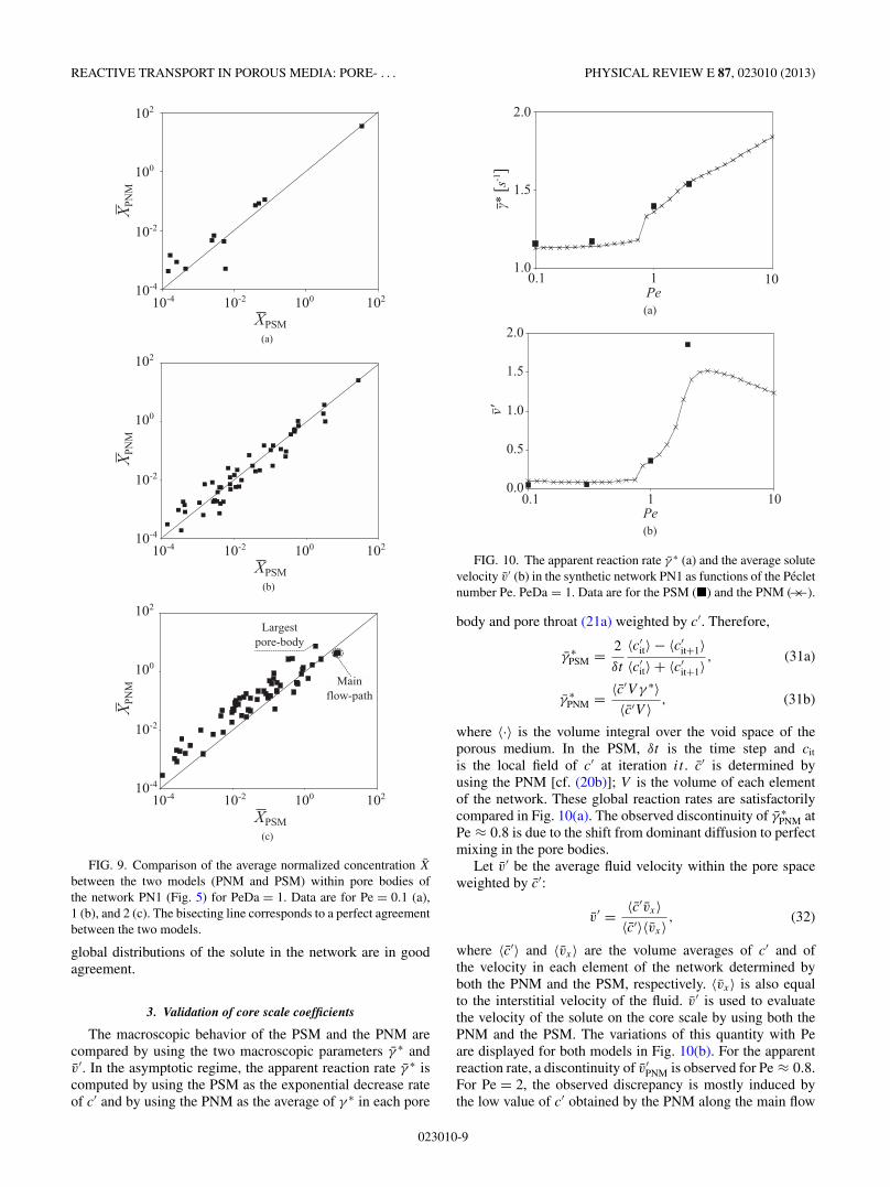
FIG. 9. Comparison of the average normalized concentration X

between the two models (PNM and PSM) within pore bodies ofthe network PN1 (Fig. 5) for PeDa = 1. Data are for Pe = 0.1 (a),1 (b), and 2 (c). The bisecting line corresponds to a perfect agreementbetween the two models.

global distributions of the solute in the network are in goodagreement.

3. Validation of core scale coefficients

The macroscopic behavior of the PSM and the PNM arecompared by using the two macroscopic parameters γ ∗ andv′. In the asymptotic regime, the apparent reaction rate γ ∗ iscomputed by using the PSM as the exponential decrease rateof c′ and by using the PNM as the average of γ ∗ in each pore

(a)

(b)

FIG. 10. The apparent reaction rate γ ∗ (a) and the average solutevelocity v′ (b) in the synthetic network PN1 as functions of the Pecletnumber Pe. PeDa = 1. Data are for the PSM (�) and the PNM ( ×−−).

body and pore throat (21a) weighted by c′. Therefore,

γ ∗PSM = 2

δt

〈c′it〉 − 〈c′

it+1〉〈c′

it〉 + 〈c′it+1〉

, (31a)

γ ∗PNM = 〈c′V γ ∗〉

〈c′V 〉 , (31b)

where 〈·〉 is the volume integral over the void space of theporous medium. In the PSM, δt is the time step and cit

is the local field of c′ at iteration it . c′ is determined byusing the PNM [cf. (20b)]; V is the volume of each elementof the network. These global reaction rates are satisfactorilycompared in Fig. 10(a). The observed discontinuity of γ ∗

PNM atPe ≈ 0.8 is due to the shift from dominant diffusion to perfectmixing in the pore bodies.

Let v′ be the average fluid velocity within the pore spaceweighted by c′:

v′ = 〈c′vx〉〈c′〉〈vx〉 , (32)

where 〈c′〉 and 〈vx〉 are the volume averages of c′ and ofthe velocity in each element of the network determined byboth the PNM and the PSM, respectively. 〈vx〉 is also equalto the interstitial velocity of the fluid. v′ is used to evaluatethe velocity of the solute on the core scale by using both thePNM and the PSM. The variations of this quantity with Peare displayed for both models in Fig. 10(b). For the apparentreaction rate, a discontinuity of v′

PNM is observed for Pe ≈ 0.8.For Pe = 2, the observed discrepancy is mostly induced bythe low value of c′ obtained by the PNM along the main flow

023010-9

VARLOTEAUX, VU, BEKRI, AND ADLER PHYSICAL REVIEW E 87, 023010 (2013)

FIG. 11. The normalized concentration c′ obtained by the PSM in PN2 for PeDa = 1. Data are for Pe = 0.1 (a), 1 (b), and 50 (c). (d) Grayscale used to display the local normalized concentration.

path where the dominant reaction takes place. Despite theassumptions made in the PNM, a good quantitative agreementbetween models is observed for the macroscopic parameters.

B. Validation of reaction regimes

The second proposed geometry, reduced to six pore bodiesin a single plane and called PN2, has been devised for a betterunderstanding of the various reaction patterns observed in theasymptotic regime. A cross section of the chosen geometry isshown in Fig. 11. Three facts are important to notice aboutthis geometry: first, the main flow path is composed of thepore bodies PB1 and PB2; second, the largest pore body PB1belongs to the main flow path; third, the largest pore body outof the main flow path, PB3, belongs to the secondary flow path.

Three local fields c′ are illustrated in Fig. 11; the crosssections of the fields using the PSM are drawn for Pe = 0.1,1, and 50 to illustrate the three reaction regimes observedat PeDa = 1. Indeed, Fig. 11(a) illustrates the first reactionregime identified for PN1, i.e., reaction occurring within thelargest pore body for low Pe. Moreover, in Fig. 11(c), adominant reaction is observed in the main flow path for veryhigh Pe. However, for an intermediate Pe (Pe = 1), a particularreaction regime is observed [Fig. 11(b)]. In this transitionalregime, reaction occurs preferentially within the largest porebody out of the main flow path.

Of course, the governing regime has important conse-quences on the value of the macroscopic parameters andon the porosity-permeability evolution. The transition regime[Fig. 11(b)] would induce a lower macroscopic velocitybecause the fluid velocity in the main flow path is faster thanin the secondary flow path where the reaction is dominant.

The variations of X in the three main pore bodies (PB1,PB2, and PB3) as a function of Pe are displayed in Fig. 12 forthe PNM and the PSM.

A perfect agreement between models is observed for Pe =0.1 in each pore body. The reaction occurs preferentially forthe two models in the largest pore body, PB1.

For Pe = 1 and Pe = 10, both PNM and PSM calculationsshow that the reaction occurs preferentially in PB3 (Fig. 12).However, small discrepancies of concentrations appear whichare due to the zero velocity assumed by the PNM inpore bodies. Nevertheless, the observed discrepancy betweenmodels remains small since the reaction mostly occurs in PB3where diffusion is still dominant for Pe � 10.

For Pe = 50, PSM calculations show that reaction occurspreferentially along the main flow path and that it induceswormholing dissolution patterns [Fig. 11(c)]; indeed, XPB1 andXPB2 are larger than XPB3, as observed in Fig. 12. Moreover,according to the PNM, the wormholing reaction regime is notfully established for Pe = 50 since the network still undergoesa dominant reaction in PB3. However, the larger Pe becomes,the more dominant the main flow path becomes until XPB1 andXPB2 overtake XPB3 for Pe ≈ 200. The observed discrepancyis due to the PNM, where the pore-body hydraulic resistanceis neglected. As a consequence, higher Pe is needed to observea dominant reaction along the main flow path in the PNM.

Therefore, it is important to notice that the same threereaction regimes are obtained by both models.

C. Discussion

1. Model complementarity

The proposed study shows a good agreement between thetwo models despite their different application scales. Thesame qualitative behavior and the same regime changes areobserved by using both models for the studied networks.Local resolution of flow and concentration allows a betterunderstanding of the limitations of PNM assumptions. Forlow Pe, a very good quantitative agreement between modelsis observed. Thus, in diffusive conditions, the simplifyingassumptions of the PNM are justified and compatible withthe exact PSM calculations.

For high Pe, the strong assumptions of the PNM relativeto pore bodies can lead to significant discrepancies in c′ whencompared to the PSM. One should notice that, generally in the

023010-10

REACTIVE TRANSPORT IN POROUS MEDIA: PORE- . . . PHYSICAL REVIEW E 87, 023010 (2013)

(a)

(b)

(c)

FIG. 12. The average normalized concentration X as a function ofPe in (a) the largest pore body (PB1), (b) the second pore body alongthe main flow path (PB2), and (c) the largest pore body out of themain flow path (PB3). Data are for the PSM (�) and the PNM (—).

PNM, the porous medium is not modeled by a regular latticealigned with the pressure gradient (θ = 0◦). This kind of pore-network construction is not able to take into account the tor-tuosity of a real porous medium. A classical way to avoid thisproblem is to consider a regular lattice rotated by θ = 45◦ withrespect to the applied pressure gradient, or to consider an irreg-ular lattice. For these porous media, the comparison betweenPSM and PNM results should be even better since the perfectmixing assumption in pore bodies would be more justified.

2. Reaction regimes

According to Daccord et al. [37], three main regimes occurduring a surface reaction depending on Pe and PeDa numbers:a uniform reaction for low PeDa, a flow path reaction forhigh PeDa and high Pe (inducing wormholing), and a compact

reaction for high PeDa and low Pe (inducing vuggy porosityformation). Thus, for high PeDa, this classification predictsa change of reaction regime with Pe, from compact reactionto wormholing. This change is confirmed by both PNM andPSM wall flux calculations performed on PN1 (Sec. IV A).The evolution of the reaction regime with Pe results from thecompetition, in terms of c′, between the largest pore body andthe main flow path. However, in PN2, where the largest porebody is on the main flow path, an intermediary reaction regimeappears between compact and wormholing reaction regimes.To the best of our knowledge, this specific regime was notobserved in the literature.

For a better understanding of conditions for this newintermediary regime to appear, the main and secondary flowpaths of PN2, denoted FPM and FPS , respectively, in Fig. 13,are independently studied by using the PNM. The flow pathwith the slowest γ ∗ is likely to dominate the solute transport.In Fig. 13(c), the reaction rates γ ∗ of FPM and FPS areplotted as functions of Pe (cf. Fig. 12); two crossing pointsare noticed (Pe ≈ 0.25 and Pe ≈ 300). Thus, for a given Pe,the local velocities in FPM and FPS are the same as in thecorresponding flow paths in PN2. For low Pe (Pe < 0.25), c′in PN2 is localized essentially in the main flow path since thereaction rate of FPM is slower than that of FPS [Fig. 13(c)];the same behavior is observed in Fig. 12. For moderatePe (0.25 < Pe < 300), c′ in PN2 is localized essentially inFPS because its reaction rate is slower than the FPM one[Fig. 13(c)]; the same behavior is also observed in Fig. 12.For high Pe (Pe > 300), c′ in PN2 is localized along FPM

because its rate is again slower than the FPS one [Fig. 13(c)],as observed in Fig. 12.

By considering only the calculations performed either onFPM or on FPS , one can notice the increase of the apparentreaction rate γ ∗ with Pe, which corresponds to an accelerationof the chemical reaction. For a better understanding of thisphenomenon, one should notice that, for high PeDa, the meanreaction rate of each element of the network (pore body or porethroat) is inversely related to the square of its radius. Indeed,for high PeDa, ω, which is the solution of (A7) [or (A12)depending on the shape of the element], tends to a constant.Thus, γ ∗, which is equal to λ in (A3), is related to the radius ofan element through (A6) (see Appendix A for more details).Therefore, the larger an element, the slower the reaction rate(because the reaction is limited by diffusion). Nevertheless,for low Pe, solute exchanges between elements are limited;each element reacts according to its own rate γ ∗. Since theelement (or group of elements) with the slowest reactionrate dominates the solute transport in the asymptotic regime,the reaction occurs in the larger pore body for low Pe. Thus,the calculated γ ∗ is slower than for any higher value of Pe.

Moreover, the exchanges of solute along FPM and FPS

increase with Pe. Thus, c′ in the largest pore body of each flowpath is convected out and consumed by the nearby pore throats.Since these elements are necessarily smaller and their reactionrate is faster, a speed up of the apparent reaction rate of theflow path is induced; for instance, this acceleration is observedin Fig. 13(c) around Pe = 1 and Pe = 100 for FPM and FPS ,respectively. Therefore, γ ∗ is an increasing function of Pe.

Finally, when convection is dominant over diffusion withinFPM or FPS (for very high Pe), the distribution of c′ is uniform

023010-11

VARLOTEAUX, VU, BEKRI, AND ADLER PHYSICAL REVIEW E 87, 023010 (2013)

(a) (b) (c)

FIG. 13. The main flow path (a) and the secondary flow path (b) of PN2. (c) The apparent reaction rate γ ∗ as a function of Pe for the main(�) and secondary (—) flow paths.

along the flow path. The obtained reaction rate, denotedγ ∗

c , is the quickest reaction rate that can be reached by theconsidered geometry. Since c′, in this case, is uniform, γ ∗

c canbe evaluated by using (31b) as the volume average of γ ∗ alongthe considered flow path (FP):

γ ∗c =

∑FP

V γ ∗/∑

FP

V . (33)

Thus, the intermediary reaction regime, highlighted by thestudy of PN2, appears when two conditions are satisfied. First,the largest pore body of the network must belong to the mainflow path. Second, at least one element of the pore networkout of the main flow path must have a reaction rate slower thanthe critical reaction rate γ ∗

c of the main flow path.Since γ ∗ is inversely related to the square of the diameter

D of the element for high PeDa, the above conditions can beformulated by using element diameters. A critical diameterDc is defined as the diameter of a pore body where the solutereacts at the same rate as on the main flow path of the network.The second condition necessitates that at least one pore bodydiameter is greater than Dc:

∀m /∈ FPM, Dm < maxFPM

D, (34a)

∃m /∈ FPM, Dm > Dc =√√√√∑

FPM

V

/∑FPM

V

D2. (34b)

Of course, these two conditions are verified in PN2. Thelargest pore body is on the main flow path with a diameterof Dmax = 65 μm; the critical diameter is Dc ≈ 55 μm andDPB3 = 60 μm is the diameter of the largest pore body out ofthe main flow path. Thus, this intermediate regime disappearswhen the diameter of PB3 is smaller than 55 μm. Figure 14shows the mean c′ calculated by using the PNM in the modifiedPN2 (PB3 = 55 μm instead of 60 μm). Whatever the value ofPe, c′ in PB1 is always higher than in the new PB3 and there isno longer an intermediate reaction regime. On the one hand, acompact reaction is observed at low Pe; diffusion is dominantin PB1 and its mean c′ is high. On the other hand, for high Pe,

the network undergoes a wormholing regime; perfect mixingis assumed in PB1 and PB3 and their c′ values are around 1.

V. APPLICATION OF THE PNM TO A PORE NETWORKEXTRACTED FROM A REAL ROCK SAMPLE

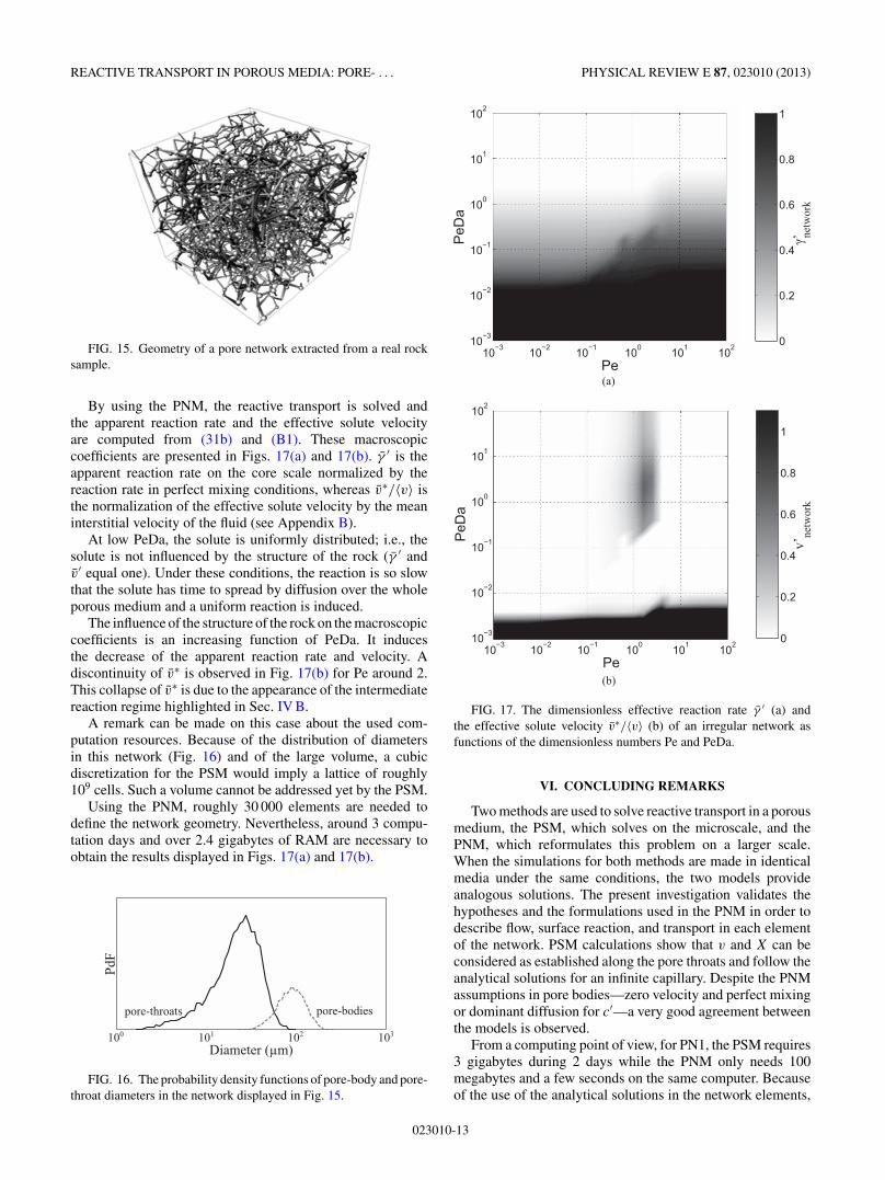
In this section, the reactive flow modeling using the PNM isapplied to an irregular 3D pore network that is extracted frommicrotomography images (Fig. 15). Due to the complexityof real porous media, the mixing in pore bodies is improvedand the local tortuosity of pore throats reduces the relativecontribution of pore bodies to permeability. Therefore, insuch a geometry, the PNM assumptions are more realistic.The imaged sample is used to calculate the macroscopiccoefficients of the reactive transport.

The studied network is extracted from a sample ofFontainebleau sandstone of (3000 μm)3 with a porosity of14.1%, an absolute permeability of 765 mD, and a formationfactor equal to 32. The selected sample is homogeneous with anaverage value of pore-body and of pore-throat diameters equalto 90 and 25 μm, respectively (Fig. 16). Only the pore structureof the Fontainebleau sandstone is taken into account. Forsimplicity, the chemical interaction at the fluid-rock interfaceis modeled by a constant and homogeneous κ .

FIG. 14. The average normalized concentration X calculated byusing the PNM in the modified PN2 as a function of Pe. In contrast tothe original PN2, the PB3 diameter is reduced in order not to satisfy(34b). Data are for PB1 (�) and PB3 (—).

023010-12

REACTIVE TRANSPORT IN POROUS MEDIA: PORE- . . . PHYSICAL REVIEW E 87, 023010 (2013)

FIG. 15. Geometry of a pore network extracted from a real rocksample.

By using the PNM, the reactive transport is solved andthe apparent reaction rate and the effective solute velocityare computed from (31b) and (B1). These macroscopiccoefficients are presented in Figs. 17(a) and 17(b). γ ′ is theapparent reaction rate on the core scale normalized by thereaction rate in perfect mixing conditions, whereas v∗/〈v〉 isthe normalization of the effective solute velocity by the meaninterstitial velocity of the fluid (see Appendix B).

At low PeDa, the solute is uniformly distributed; i.e., thesolute is not influenced by the structure of the rock (γ ′ andv′ equal one). Under these conditions, the reaction is so slowthat the solute has time to spread by diffusion over the wholeporous medium and a uniform reaction is induced.

The influence of the structure of the rock on the macroscopiccoefficients is an increasing function of PeDa. It inducesthe decrease of the apparent reaction rate and velocity. Adiscontinuity of v∗ is observed in Fig. 17(b) for Pe around 2.This collapse of v∗ is due to the appearance of the intermediatereaction regime highlighted in Sec. IV B.

A remark can be made on this case about the used com-putation resources. Because of the distribution of diametersin this network (Fig. 16) and of the large volume, a cubicdiscretization for the PSM would imply a lattice of roughly109 cells. Such a volume cannot be addressed yet by the PSM.

Using the PNM, roughly 30 000 elements are needed todefine the network geometry. Nevertheless, around 3 compu-tation days and over 2.4 gigabytes of RAM are necessary toobtain the results displayed in Figs. 17(a) and 17(b).

FIG. 16. The probability density functions of pore-body and pore-throat diameters in the network displayed in Fig. 15.

(a)

(b)

FIG. 17. The dimensionless effective reaction rate γ ′ (a) andthe effective solute velocity v∗/〈v〉 (b) of an irregular network asfunctions of the dimensionless numbers Pe and PeDa.

VI. CONCLUDING REMARKS

Two methods are used to solve reactive transport in a porousmedium, the PSM, which solves on the microscale, and thePNM, which reformulates this problem on a larger scale.When the simulations for both methods are made in identicalmedia under the same conditions, the two models provideanalogous solutions. The present investigation validates thehypotheses and the formulations used in the PNM in order todescribe flow, surface reaction, and transport in each elementof the network. PSM calculations show that v and X can beconsidered as established along the pore throats and follow theanalytical solutions for an infinite capillary. Despite the PNMassumptions in pore bodies—zero velocity and perfect mixingor dominant diffusion for c′—a very good agreement betweenthe models is observed.

From a computing point of view, for PN1, the PSM requires3 gigabytes during 2 days while the PNM only needs 100megabytes and a few seconds on the same computer. Becauseof the use of the analytical solutions in the network elements,

023010-13

VARLOTEAUX, VU, BEKRI, AND ADLER PHYSICAL REVIEW E 87, 023010 (2013)

the PNM can be applied to large velocities and reaction rates.However, this approach cannot represent exactly the geometryand the local evolutions of the solute. The PNM only providesan average description of solute distribution in pore bodies andpore throats. Because of the simplifications used in the PNM,a large volume can be addressed with affordable computationresources.

A new reaction regime, not mentioned in the literature, isbrought into light which depends on the localization and thediameter of the largest elements of the porous medium withrespect to the main flow path. This new reaction regime canhave consequences on the macroscopic behavior of the solutewhich can change the distribution pattern of the concentrationin reservoir simulators [38].

APPENDIX A: ANALYTICAL RESOLUTION OFTHE TRANSVERSE PROFILE

This Appendix is devoted to the resolution of reactivetransport in infinite capillary tubes and in closed spheres. Asa reminder, the reactive transport of a solute is governed by

Pe∇′c′ · v′ − ∇′2c′ = − L2

DT

∂c′

∂tin �F , (A1)

n · ∇′c′ = −PeDa c′ on �. (A2)

1. Infinite capillary tube

In the asymptotic regime, (A1) becomes a well-knownsecond-order ordinary differential equation because c′(ρ,t) isdecomposed as

c′(ρ,t) = X(ρ) exp(−λt). (A3)

For an infinite cylinder, the local problem is governed by

1

ρ ′d

dρ ′

(ρ ′ dX

dρ ′

)+ λr2

DX(ρ ′) = 0, (A4)

whose solutions are linear combinations of Bessel functionsof first and second kinds (commonly denoted J0 and Y0,respectively), where r is the radius of the cylinder and ρ ′is the dimensionless radial coordinate (ρ ′ = ρ/r). However,Y0 is discontinuous at zero, which is not compatible with thecontinuity of the concentration profile. Thus, the normalizedconcentration profile is

X(ρ ′) = aJ0(ωρ ′), (A5)

where ω is a dimensionless factor related to the exponentialdecrease rate λ; ω depends on the surface reaction rate.Indeed, by substitution of (A5) into (A4), the following relationbetween ω and λ is obtained:

λ = Dω2

r2. (A6)

Moreover, by substituting the local solution (A5) into theboundary condition equation (A2), a relation can be deducedbetween ω and the local PeDa of the cylinder:

ωJ1(ω)

J0(ω)= κr

D= PeDa. (A7)

Since a general analytical solution of this equation does notexist, ω must be numerically determined for a given PeDa.In order to deal with a dimensionless profile X(ρ ′), its meanvalue over a section of the cylinder is fixed to 1. This leads tothe final expression of X for a cylinder:

X(ρ ′) = ω2

2PeDa

J0(ωρ ′)J0(ω)

. (A8)

2. Closed sphere

Within a closed sphere, the local problem can be written as

1

ρ ′2d

dρ ′

(ρ ′2 dX

dρ ′

)+ λR2

DX(ρ ′) = 0, (A9)

where R is the radius of the sphere and ρ ′ is the dimensionlessradial coordinate (ρ ′ = ρ/R). The physical solution of thisequation is

X(ρ ′) = asin(ωρ ′)

ωρ ′ . (A10)

By substituting Eq. (A10) into (A9), an analogous relation to(A6) is obtained:

λ = Dω2

R2. (A11)

Since the same reasoning can be used for the boundarycondition, the following relation is deduced:

1 − ω

tan ω= κR

D= PeDa. (A12)

Similarly to the cylinder geometry, the determination ofω requires a numerical evaluation for a given PeDa. Thefinal expression of X within a closed sphere is obtained bynormalizing the mean concentration over the whole sphere:

X(ρ ′) = ω2

3PeDa

sin(ωρ ′)ρ ′ sin(ω)

. (A13)

APPENDIX B: MACROSCOPIC SOLUTE VELOCITY

According to Shapiro and Brenner [39], the macroscopicvelocity of the solute v∗ can be expressed as

v∗ = 〈X0Y0v + D(Y0∇X0 − X0∇Y0)〉〈X0Y0〉 , (B1)

where X0 and Y0 are the solutions of the local reactivetransport problem and its adjoint problem, respectively. Thisexpression is adapted to the PNM as proposed by Varloteauxet al. [38]. The macroscopic velocity of the solute is used torepresent the advective contribution of the reactive transportat a macroscopic scale. Of course, this velocity is not equal tov′ defined in Sec. IV A.

023010-14

REACTIVE TRANSPORT IN POROUS MEDIA: PORE- . . . PHYSICAL REVIEW E 87, 023010 (2013)

[1] O. Izgec, B. Demiral, H. Bertin, and S. Akin, Transp. PorousMedia 72, 1 (2008).

[2] O. Izgec, B. Demiral, H. Bertin, and S. Akin, Transp. PorousMedia 73, 57 (2007).

[3] S. Bekri, J.-F. Thovert, and P. Adler, Chem. Eng. Sci. 50, 2765(1995).

[4] C. L. Phillips, MIT Undergrad. J. Math. 1, 155 (1999).[5] J. A. Sethian and P. Smereka, Annu. Rev. Fluid Mech. 35, 341

(2003).[6] A. C. Payatakes and M. M. Dias, Rev. Chem. Eng. 2, 85 (1984).[7] B. W. Lindquist, A. Venkatarangan, J. Dunsmuir, and T.-F.

Wong, J. Geophys. Res. 105, 21509 (2000).[8] C. Laroche and O. Vizika, Transp. Porous Media 61, 77 (2005).[9] A. Al-Kharusi and M. Blunt, J. Petrol. Sci. Eng. 56, 219 (2007).

[10] A. Raoof and S. Hassanizadeh, Transp. Porous Media 81, 391(2009).

[11] Q. Kang, P. C. Lichtner, H. S. Viswanathan, and A. I. Abdel-Fattah, Transp. Porous Media 82, 197 (2009).

[12] I. Fatt, Trans. AIME 207, 144 (1956).[13] M. Blunt, D. Zhou, and D. Fenwick, Transp. Porous Media 20,

77 (1995).[14] M. I. J. van Dijke and K. S. Sorbie, Phys. Rev. E 66, 046302

(2002).[15] P. Øren, J. Petrol. Sci. Eng. 39, 177 (2003).[16] C. Lu and Y. C. Yortsos, Ind. Eng. Chem. Res. 43, 3008 (2004).[17] J. Ochi, Transp. Porous Media 37, 303 (1999).[18] M. Sahimi, A. R. Mehrabi, N. Mirzaee, and H. Rassamdana,

Transp. Porous Media 41, 325 (2000).[19] S. Bhat, in SPE Western Regional Meeting (Bakersfield, USA,

1998), p. 46210.[20] C. Lu and Y. C. Yortsos, Phys. Rev. E 72, 036201 (2005).[21] A. Raoof, S. M. Hassanizadeh, and A. Leijnse, Vadose Zone J.

9, 624 (2010).[22] L. Li, C. A. Peters, and M. Celia, Adv. Water Resour. 29, 1351

(2006).

[23] D. Kim, Scale-up of reactive flow through network flow mod-elling (State University of New York at Stony Brook, New York,USA, 2009).

[24] L. Algive, S. Bekri, M. Robin, and O. Vizika, in Proceeding ofthe International Symposium of the Society of Core Analysts, 10(SCA, Calgary, 2007).

[25] L. Algive, S. Bekri, and O. Vizika, SPE J. 15, 618 (2010).[26] J. A. Sethian, Proc. Nat. Acad. Sci. USA 93, 1591 (1996).[27] C. Lu and Y. C. Yortsos, AIChE J. 51, 1279 (2005).[28] S. Bekri and O. Vizika, in Proceeding of the International Sym-

posium of the Society of Core Analysts, 22 (SCA, Trondheim,2006).

[29] S. Youssef, E. Rosenberg, N. Gland, S. Bekri, and O. Vizika,in Proceeding of the International Symposium of the Society ofCore Analysts, 17 (SCA, Calgary, 2007).

[30] P. E. Øren and S. Bakke, Transp. Porous Media 46, 311(2002).

[31] R. Sok, M. Knackstedt, A. Sheppard, W. Pinczewski, W.Lindquist, A. Venkatarangan, and L. Paterson, Transp. PorousMedia 46, 345 (2002).

[32] J.-F. Thovert, J. Salles, and P. M. Adler, J. Microsc. 170, 65(1993).

[33] W. H. Press, B. P. Flannery, S. A. Teukolsky, and W. T. Vetterling,Numerical Recipes in C: The Art of Scientific Computing, 2nded. (Cambridge University Press, Cambridge, England, 1992).

[34] R. Sankarasubramanian and W. N. Gill, Proc. R. Soc. London,Ser. A 333, 115 (1973).

[35] M. Shapiro and H. Brenner, Chem. Eng. Sci. 41, 1417(1986).

[36] H. Brenner, Philos. Trans. R. Soc. London A 297, 81 (1980).[37] G. Daccord, O. Lietard, and R. Lenormand, Chem. Eng. Sci. 48,

179 (1993).[38] C. Varloteaux, S. Bekri, and P. M. Adler, Adv. Water Resour.

53, 87 (2013).[39] M. Shapiro and H. Brenner, Chem. Eng. Sci. 43, 551 (1988).

023010-15