reactive transport for fuel containing materials · conceptual model ⇓ quantification...
TRANSCRIPT

Report T14 / R23
Reactive Transport for
Fuel Containing Materials
(Dynamical Compartment Model)
to
Chernobyl NPP Unit 4 – SIP EBP Package “D”
submitted by
UIT GmbH Dresden, Germany
September 2000
kin
outflow
inflow
primaryphases
mobilewater
secondaryphases
stagnantwater
diff
eq
Umwelt- und Ingenieurtechnik GmbH Dresden
Modeling FCM – Chernobyl NPP
I
Report to
Chernobyl NPP Unit 4 – SIP EBP Package “D”
Task 14 / R23 (Predicted Data Changes)
Reactive Transport for
Fuel Containing Materials
– Dynamical Compartment Model –
H. KALKA
September 2000

Umwelt- und Ingenieurtechnik GmbH Dresden
Modeling FCM – Chernobyl NPP II
Contents page 1 1.1 1.2 1.2.1 1.2.2
Introduction Objectives and Background List of Abbreviations, Terms and Symbols List of Abbreviations List of Mathematical Symbols
11444
2 Conceptual Model 62.1 2.1.1 2.1.2 2.1.3 2.2 2.2.1 2.2.2 2.2.3 2.2.4 2.3 2.3.1 2.3.2 2.3.3 2.3.4 2.3.5
Basic Idea Dual-Zone Structure of a Compartment Types of Fuel Containing Masses Other Mass Types (Primary Phases) Compartment Structure of “Chernobyl Shelter” Geometrical Structure External Water Flow Condensation and Evaporation Internal Water Flow Chemical Processes Kinetics versus Thermodynamic Equilibrium Components of Shelter Waters Chemical Transformations inside a Compartment Relations between Kinetic Parameters for FCM Example: Water Percolation through the Shelter
669
101111121415161618192222
3 Mathematical Model 233.1 3.1.1 3.1.2 3.1.3 3.2 3.3 3.3.1 3.3.2 3.3.3 3.4 3.4.1 3.4.2 3.4.3 3.4.4
Basic Equations Advection-Reaction Equation Flow Equation and Flow Field Linkage between Flow and Transport Numerical Model Sink/Source Term Diffusion and Dissolution Processes First-Order Kinetics Water-Solid Equilibrium Dynamics of Phase Transformations Interacting Subsystems Final Expressions and Model Parameters Special Case: Dissolution of Hot Particles Local and Global Mass Balance
2424252627282830303131323334
4 Data Preparation and Model Calibration 34

Umwelt- und Ingenieurtechnik GmbH Dresden
Modeling FCM – Chernobyl NPP
III
page4.1 4.2 4.2.1 4.2.2 4.2.3 4.3 4.3.1 4.3.2
Input Data Structure Model Parameters Thermodynamic Data Kinetic Data Dissolution Rate for Hot Particles Model Calibration Calibration Strategy Example: Dissolution of Hot Particles
3435353637383839
5 Summary and Outlook 39 References i

Umwelt- und Ingenieurtechnik GmbH Dresden
Modeling FCM – Chernobyl NP 1
1 Introduction
1.1 Objectives and Background Objectives. This report presents a model concept for the dynamical description of the chemi-cal weathering of fuel containing materials (FCM), construction materials (CM), and dump-ing materials (DM) due to the influence of water and atmosphere. To simulate the migration of uranium in aqueous form and its redistribution in the Shelter the model combines mass transport with reactions including both equilibrium processes (thermodynamics) and kinetics. Based on the conceptual model this report includes the mathematical derivation of the main equations and identifies the input data as well as the most influencing parameters for a straightforward calculation. The route from the conceptual model to the numerical model de-scribed in this report is as follows: Conceptual Model
⇓ quantification Mathematical Model
⇓ spatial and temporal discretization
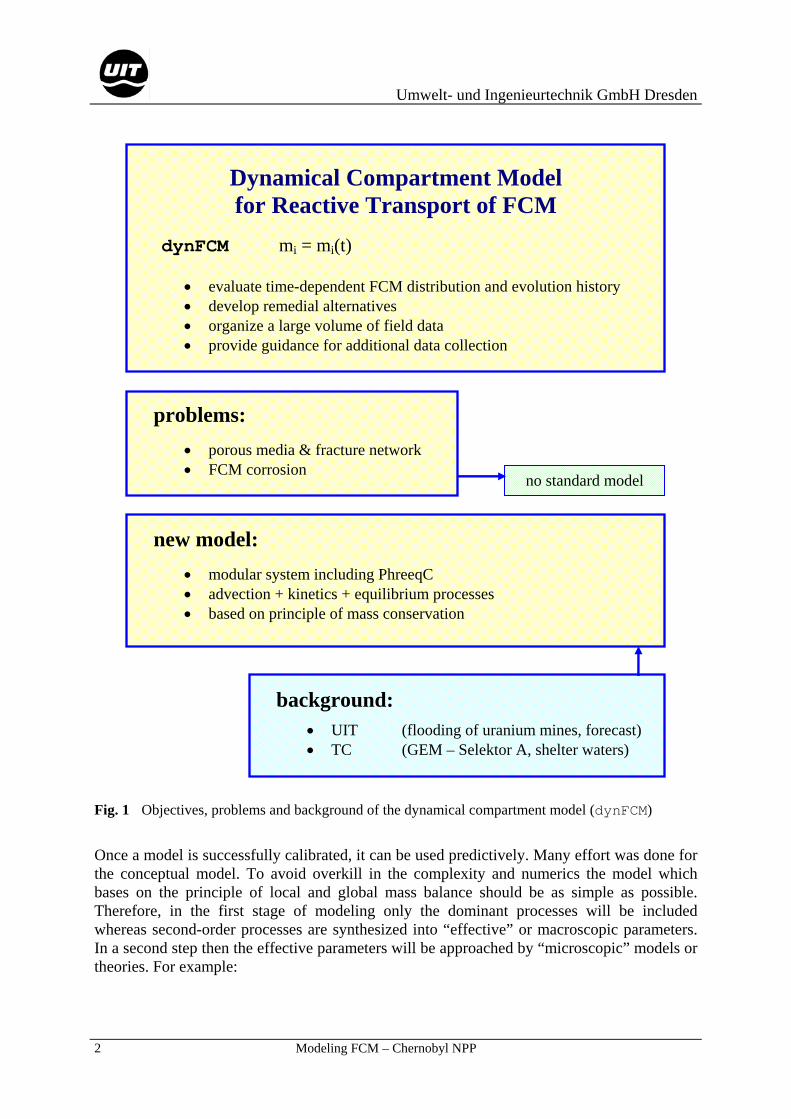
Numerical Model (code dynFCM) After model construction and model calibration the compartment model becomes a tool for forecast and for dynamical simulation of different leaching scenarios within the Chernobyl Shelter. In this way the reactive transport model is useful to (see Fig. 1):
• evaluate the time-dependent FCM distribution and evolution history, • develop Shelter water management strategy (remedial alternatives), • organize a large volume of field data, • provide guidance for additional data collection.
In case of application of active leaching technologies for FCM removal (see T20/D1-report and its appendix) this model could be useful for selecting optimized removal strategies and for the interpretation of the demonstration (pilot) experiments. Generalized Modeling Approach. A variety of tasks are required in construction of a dy-namical Shelter model. The main steps include:
• the development of a conceptual model (Chapter 2), • the creation of the mathematical model (Chapter 3), • the definition of the input data structure and specification of the model parameters, • its realization as a software package dynFCM for Windows-based personal computers, • model calibration and validation testing by execution of various trials.
Umwelt- und Ingenieurtechnik GmbH Dresden
2 Modeling FCM – Chernobyl NPP
Fig. 1 Objectives, problems and background of the dynamical compartment model (dynFCM)
Once a model is successfully calibrated, it can be used predictively. Many effort was done for the conceptual model. To avoid overkill in the complexity and numerics the model which bases on the principle of local and global mass balance should be as simple as possible. Therefore, in the first stage of modeling only the dominant processes will be included whereas second-order processes are synthesized into “effective” or macroscopic parameters. In a second step then the effective parameters will be approached by “microscopic” models or theories. For example:
Dynamical Compartment Model for Reactive Transport of FCM
dynFCM mi = mi(t)
• evaluate time-dependent FCM distribution and evolution history • develop remedial alternatives • organize a large volume of field data • provide guidance for additional data collection
problems:
• porous media & fracture network • FCM corrosion
new model:
• modular system including PhreeqC • advection + kinetics + equilibrium processes • based on principle of mass conservation
no standard model
background:
• UIT (flooding of uranium mines, forecast) • TC (GEM – Selektor A, shelter waters)
Umwelt- und Ingenieurtechnik GmbH Dresden
Modeling FCM – Chernobyl NP 3
1st stage: main processes (FCM-water system and CM-water-system) and main elements (Na, K, Ca, Mg, Cl, S, C, H, O, Fe, Al, U),
2nd stage: “second-order processes” (Zr-U-O phases, etc.) and complete element spec-trum including all radionuclides,
[3rd stage: LFCM destruction and dust production (hot particles) including aerosol-transport within the shelter. ]
The present report describes all procedures and parameters to realize the 1st stage. Background. For the numerical treatment of the advection-reaction processes within the highly complex and heterogeneous system “Shelter” there is no standard model or software package available. The well-known code families for transport and reactive transport [DS98] are not adequate tools to describe the processes within the Shelter because of the complicated – and in most cases unknown – combinations of flow through porous media and through frac-ture networks. Therefore a new dynamical approach for an “average” or “effective” descrip-tion of the problem is appropriate. For this reason – based on existing experiences, observed data, and software tools – a Shelter-specific dynamical model for reactive transport of FCM will be developed. The main experi-ences are:
First. In the last years UIT has developed a special software package for the consistent simu-lation of the hydrological and geochemical conditions in great heterogeneous and complex systems (flooding of Uranium mines in Saxonia, Thuringia, Colorado; long-term forecast, kinetic oxidation processes, etc.) [Ka98, Pau98, UIT00, and about 15 internal reports] which includes the chemical code PhreeqC [Par95] as a special subroutine to calculate the (equilib-rium) processes. The kinetics for dissolution / precipitation and other non-equilibrium proc-esses are treated separately in time steps of size ∆t. Second. Since 1991 at Technocentre in Kiev thermodynamic evaluation and studies of the interaction of Shelter waters with FCM and CM based on a convex programming approach to Gibbs free energy minimization (Selektor-A code) are performed [Sin97, Sin98, Ku98]. These investigations establish the stabile phases as well as the appropriate equilibrium constants (log-k values) which are necessary for equilibrium calculations with PhreeqC. Finally, all available information’s from other SIP documents are used: Task 10 [T10], Task 13 [T13], and Task 14 [T14]. Modular software design. The model dynFCM will be build with a modular design that con-sists of a main program and “packages”. The packages – most of them already exist – are groups of independent subroutines that carry out specific simulation tasks such as transport, kinetics, diffusion, equilibrium calculations with PhreeqC etc. This modular design is useful in several ways. It provides a logical basis for organizing the actual code with similar pro-gram elements or functions grouped together. Such a structure facilitates the integration of new packages to enhance the code’s capabilities.

Umwelt- und Ingenieurtechnik GmbH Dresden
4 Modeling FCM – Chernobyl NPP
The software is written in the object oriented programming language C++ which goes along with the ideas of modular design [St94]. 1.2 List of Abbreviations, Terms and Symbols
1.2.1 List of Abbreviations CF Core Fragments CM Construction Materials (concrete, steel) CSH Amorphous Calcium Silicate Hydrogel Phase DM Materials dumped by helicopters to smoother the reactor fire during the “Ac-
tive phase Accident Management Actions” (Na3PO4, dolomite, ...) FCM Fuel Containing Materials HP Hot Particles IAP Ion Activation Product LFCM Lava-like Fuel Containing Materials NIAS Nuclear Island Auxiliary System SUM Secondary Uranium Minerals TST Transition-State Theory Computer Codes dynFCM software package of the Dynamical Compartment Model for Reactive Trans-
port of FCM within the Shelter (the object of this report) PhreeqC Program for Geochemical Calculations from U.S. Geological Survey [Par95,
PA99] Selektor-A Convex programming approach to Gibbs Free Energy Minimization, Techno-
centre Kiev Physical Units: L length (m) T time (s) M mass (kg or mol) [Note that the abbreviation for the length L and the abbreviation for the volume unit liter (L) is the same, 1 L = 1 dm3. The actual meaning becomes clear from context.] The molar concentrations of chemical species are also symbolized by brackets: [H2O], [U], etc. 1.2.2 List of Mathematical Symbols To give a mathematical foundation of the model a lot of symbols should be defined. The sub-scripts i and j refer to the compartment i and j. So-called global quantities are independent of i and/or j. In general, all concentrations c and masses m are vectors of K species (for example:
)k(ic denotes the concentration of species k in compartment i, with 1 ≤ k ≤ K). However, to
keep the notation as simple as possible the superscripts k will be dropped.

Umwelt- und Ingenieurtechnik GmbH Dresden
Modeling FCM – Chernobyl NP 5
a thickness of the stationary layer L iA base area of compartment i L2 DiA surface of “diffusion layer” L2 SiA (initial) surface area of the solid which is in water contact L2
sA si
Si m/A= , specific surface area (in m2/g) L2M-1
ic concentration in the mobile aqueous phase ML-3
ic~ concentration in the stagnant aqueous phase ML-3 eqc concentration in equilibrium with solid phase ML-3 0c pure water concentration (H2O = 55.5 mol/l) ML-3 0c concentration of external inflow water (pristine water) ML-3
D diffusion coefficient L2T-1 Eh redox potential mV fij hydraulic mixing factors between compartment i and j 1 Hi height of compartment i L k thermodynamic equilibrium constant kij splitting factor for flow paths between compartment i and j 1 i compartment number (or label) 0 ≤ i ≤ N
iiaqi Vcm = element mass in the mobile aqueous phase (bulk water) M
iiaqi V~c~m~ = element mass in the stagnant aqueous phase (pore water) M sim element mass in the solid phase M 1s
im element mass in the solid phase of primary mineral M 2s
im element mass in the solid phase of secondary mineral M n porosity L3/L3 N total number of compartments 1
ingrQ water ingress to the Shelter L3T-1 egrQ water egress from the Shelter L3T-1
jiQ → hydraulic flow rate from compartment i to compartment j L3T-1 inext
iQ external inflow rate to compartment i L3T-1 outext
iQ external outflow rate from compartment i L3T-1 inint
iQ internal inflow rate to compartment i L3T-1 outint
iQ internal outflow rate from compartment i L3T-1 iniQ external plus internal inflow rate to compartment i L3T-1 outiQ external plus internal outflow rate from compartment i L3T-1 cndiQ condensation rate in compartment i L3T-1 evpiQ evaporation rate in compartment i L3T-1
r specific rate for dissolution ML-2T-1 iR source term rate for compartment i ML-3T-1 DiR diffusion rate ML-3T-1 SiR overall reaction rate for dissolution ML-3T-1

Umwelt- und Ingenieurtechnik GmbH Dresden
6 Modeling FCM – Chernobyl NPP
iV volume of mobile water (bulk water) in compartment i L3
iV~ volume of stagnant water (pore water) in compartment i L3 RiV reaction volume L3 SiV “reactive” water volume in contact with the solid L3 DiV volume of “diffusion layer” (between stagnant and mobile water) L3
zi bottom elevation of compartment i (above sea level) L δ(t) Dirac’s delta-function T-1
Θ(x) Heaviside step-function 1
θ volumetric water content (≤ porosity n) L3/L3 ρs bulk density of the solid ML-3 κ parameter for first-order kinetics T-1
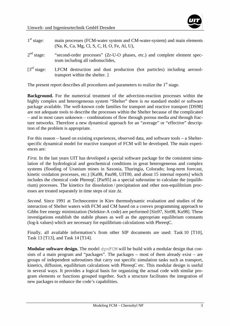
2 Conceptual Model The compartment model is based on a coarse spatial discretization of the model space (system of compartments) and fine temporal discretization (∆t in order of hours). Since there is no complete information about the transport and reaction processes on a “microscopic” scale the compartment model describes the processes in an average manner using effective parameters which will be adjusted to observed data (model calibration). This Chapter contains the model concept; the mathematical model which is based on the principle of mass conservation will be derived in Chapter 3. 2.1 Basic Idea The model space “Shelter” is divided into N compartments or regions (see Fig. 2). The com-partments are coupled by hydraulic flows (internal couplings between an arbitrary number of other compartments and external couplings between a compartment and the outside). In con-trast to the 3D hydrogeology models which are based on a fine-size grid of cells the com-partment model is quasi-3D. [Here the term compartment rather than cell is used to distinguish the present model from transport models used in geohydrology which are based on grid structures. Synonyms for compartment are box, region or domain.] 2.1.1 Dual-Zone Structure of a Compartment To describe reactive transport phenomena each compartment is conceptualized as consisting of two distinctive zones (see also Fig. 4):
transport zone T: for the mobile phases (mobile water, gas), reaction zone R: for the immobile phases (stagnant water, solids, surfaces).
Zone T is responsible for the transport (advection), i. e., the mass transfer between neighbor compartments and from/to the outside of shelter. In the reaction zone R the interaction be-

Umwelt- und Ingenieurtechnik GmbH Dresden
Modeling FCM – Chernobyl NP 7
tween stagnant water (pore solutions) and solid phases takes place. Both zones are connected by mass transfer due to diffusion between stagnant water and mobile water. [The stagnant water should not be confused with the water pools in the rooms inside the Shel-ter. In this context stagnant water signifies the pore water or the thin water film surrounding the solid phases – see Fig. 3. On the other hand, the water pools contain excess water which belongs in the present notation to the mobile water phase or so-called bulk water and which volume is in general time-dependent.]
Fig. 2 Decomposition of the model space “Shelter” into N compartments
To illustrate the dual-zone concept, Fig. 3 shows a piece of porous media. The interconnected and sufficiently large pore spaces form preferential flow pathways for mobile waters while dead-end and small pore spaces are filled with immobile waters. The immobile water is in direct contact with the solid matrix and causes its dissolution. The increased concentration in the immobile water phase then gives rise to the diffusion of solutes into the mobile water phase.
Fig. 3 Mobile and immobile phases in a piece of porous media
The lower part of Fig. 4 shows the fol-lowing processes more abstractly: First, the kinetic dissolution of a primary phase is treated as
model space „shelter“
compartment 1 compartment 2 compartment N ...
reaction zone R
(immobile phases)
transport zone T (mobile phases)
reaction zone R
(immobile phases)
transport zone T (mobile phases)
reaction zone R
(immobile phases)
transport zone T (mobile phases)
gas phase
mobile water
stagnant water
solid phase
Umwelt- und Ingenieurtechnik GmbH Dresden
8 Modeling FCM – Chernobyl NPP
a surface controlled two-step process (here two parallel dissolution paths are considered such as discussed in [Ca94], respectively) which increases the concentrations in the pore solution. The pore solution – that is the stagnant water phase – is assumed to be in equilibrium with secondary mineral phases which allows precipitation as a rate limiting process. Due to diffu-sion there is a mass exchange between both the stagnant and mobile water phases. Finally, the advection in the mobile water phase transports the mass to other compartments and/or to the environment.
Fig. 4 Example for a small complex of compartments and the internal structure of one compartment [Model of surface-controlled dissolution: The kinetics of surface-controlled dissolution is treated as a two-step process. The first step involves a rapid, reversible sorption of reactive chemical species (protons, ligands, reduc-tans) from solution onto the surface. The second step results in detachment of a metal from the surface of the crystalline lattice. The rate law for surface-controlled dissolutions is based on the assumption that the first step is fast and the second step rate-limiting. Rapid regeneration of the surface and reequilibration of the reactive sur-face species is assumed.] The aim is now to apply and modify this model framework to the special case of the Cherno-byl Shelter. Therefore, in the subsequent Sections and Chapters the main mechanisms and transformation steps will be defined. For the first model version there are at least two main assumptions:
inflow
immobilephases
mobilephases
reac
tion
zone
R
transport zone T
outflow
one compartment
reactive transport
R T
R TR T
system ofcompartments
primaryphases
surface(fast)
surface(slow)
stag-nant
water
secondary phases
mobilewater
Umwelt- und Ingenieurtechnik GmbH Dresden
Modeling FCM – Chernobyl NP 9
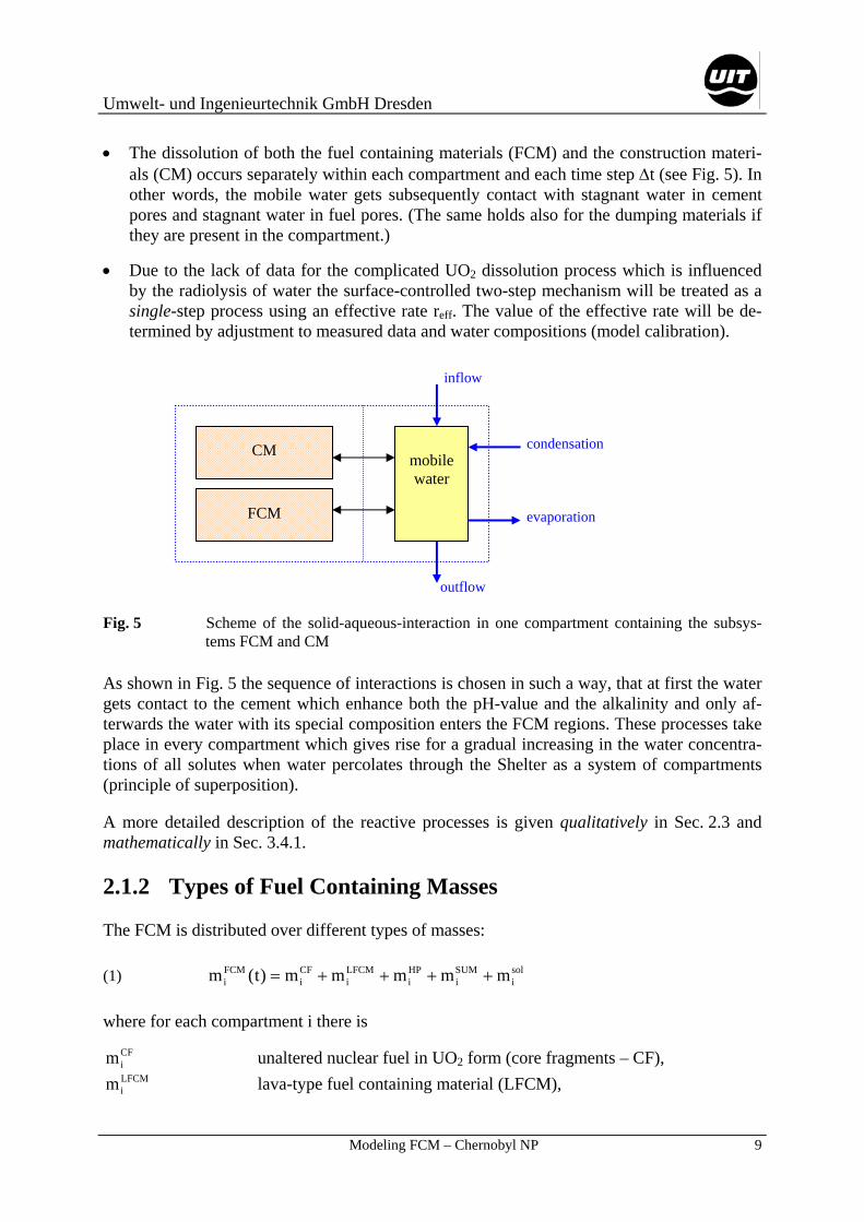
• The dissolution of both the fuel containing materials (FCM) and the construction materi-als (CM) occurs separately within each compartment and each time step ∆t (see Fig. 5). In other words, the mobile water gets subsequently contact with stagnant water in cement pores and stagnant water in fuel pores. (The same holds also for the dumping materials if they are present in the compartment.)
• Due to the lack of data for the complicated UO2 dissolution process which is influenced by the radiolysis of water the surface-controlled two-step mechanism will be treated as a single-step process using an effective rate reff. The value of the effective rate will be de-termined by adjustment to measured data and water compositions (model calibration).
Fig. 5 Scheme of the solid-aqueous-interaction in one compartment containing the subsys-tems FCM and CM
As shown in Fig. 5 the sequence of interactions is chosen in such a way, that at first the water gets contact to the cement which enhance both the pH-value and the alkalinity and only af-terwards the water with its special composition enters the FCM regions. These processes take place in every compartment which gives rise for a gradual increasing in the water concentra-tions of all solutes when water percolates through the Shelter as a system of compartments (principle of superposition). A more detailed description of the reactive processes is given qualitatively in Sec. 2.3 and mathematically in Sec. 3.4.1. 2.1.2 Types of Fuel Containing Masses The FCM is distributed over different types of masses:
(1) soli
SUMi
HPi
LFCMi
CFi
FCMi mmmmm)t(m ++++=
where for each compartment i there is
CFim unaltered nuclear fuel in UO2 form (core fragments – CF), LFCMim lava-type fuel containing material (LFCM),
condensation
evaporation
outflow
inflow
CM mobile water
FCM
Umwelt- und Ingenieurtechnik GmbH Dresden
10 Modeling FCM – Chernobyl NPP
HPim dispersed fuel in form of “hot particles” up to 10 – 40 µm (HP), SUMim secondary uranium minerals,
aqi
aqi
soli m~mm += FCM in solutions (mobile plus stagnant aqueous phases).
Here, the aqueous phase is decomposed into a stagnant phase (thin film surrounding the mate-rials, pore solutions) and a mobile phase (water which transports solutes within the Shelter, initially pristine or rain water). In this way, the first four terms in Eq. (1) represent the immo-bile inventory, whereas only the last term includes the mobile inventory in form of the mobile aqueous phase. The lava (LFCM) is a result of high temperature interaction of nuclear fuel with structures of the reactor block (backfilling materials: clay, sand, dolomite, boron, carbide, lead). The ma-trix of LFCM is a silicat glass (> 65 wt. % of SiO2) containing K, Ca, Mg, Al, U, Zr impuri-ties with no more than 3 – 4 % of each element. The composition of HP varies according to the percentage of UO2+x and different components of the structural minerals (Fe, Zr, Si etc.) up to the pure UO2. Additionally, there are different oxidation states of UO2, that is x < 0. Whereas CF, LFCM and HP are so-called primary phases the SUM represents the secondary phases. As time evolves mass from the primary phases dissolutes and will be accumulated in both secondary minerals (SUM) and solutions; the outflow to the environment proceeds then via the solution transport. The mass distribution in Eq. (1) is time dependent due to corrosion and alteration processes. In general there are various physico-chemical transformation paths for FCM:
• unaltered fuel (CF) corrosion path, • LFCM corrosion path, • HP dissolution, • evaporation path, • dust production.
2.1.3 Other Mass Types (Primary Phases) To simulate the origin and the history of Shelter waters it is necessary to consider the interac-tions with construction materials (CM) such as concrete and with the material dumped from helicopters (DM): for example 2 500 t trinatriphosfatum Na3PO4 and 800 t dolomite [Sich94]. Thus, trinatriphosfatum enhances the Na and PO4 content in the Shelter water. The interaction of pristine water with concrete generates an alkaline and carbonate solution with a relatively law redox potential of Eh ≈ -100 mV. 2.2 Compartment Structure of “Chernobyl Shelter”
Umwelt- und Ingenieurtechnik GmbH Dresden
Modeling FCM – Chernobyl NP 11
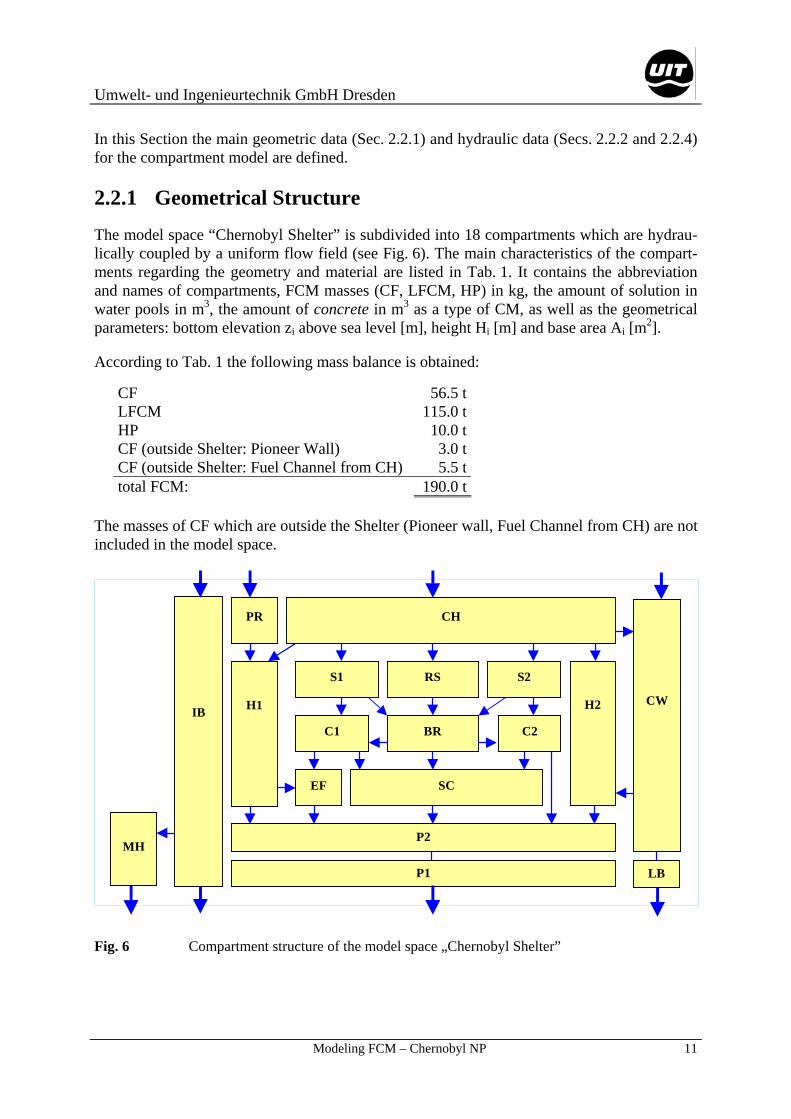
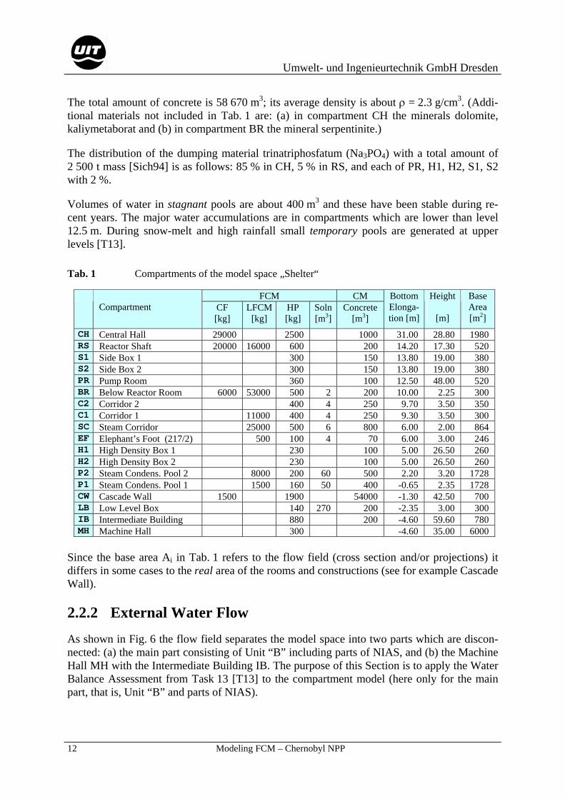
In this Section the main geometric data (Sec. 2.2.1) and hydraulic data (Secs. 2.2.2 and 2.2.4) for the compartment model are defined. 2.2.1 Geometrical Structure The model space “Chernobyl Shelter” is subdivided into 18 compartments which are hydrau-lically coupled by a uniform flow field (see Fig. 6). The main characteristics of the compart-ments regarding the geometry and material are listed in Tab. 1. It contains the abbreviation and names of compartments, FCM masses (CF, LFCM, HP) in kg, the amount of solution in water pools in m3, the amount of concrete in m3 as a type of CM, as well as the geometrical parameters: bottom elevation zi above sea level [m], height Hi [m] and base area Ai [m2]. According to Tab. 1 the following mass balance is obtained:
CF 56.5 tLFCM 115.0 tHP 10.0 tCF (outside Shelter: Pioneer Wall) 3.0 tCF (outside Shelter: Fuel Channel from CH) 5.5 ttotal FCM: 190.0 t
The masses of CF which are outside the Shelter (Pioneer wall, Fuel Channel from CH) are not included in the model space.
Fig. 6 Compartment structure of the model space „Chernobyl Shelter”
CHPR
IB H1
RS
H2
LBP1
MH
BR
EF SC
P2
S1 S2
C1 C2
CW
Umwelt- und Ingenieurtechnik GmbH Dresden
12 Modeling FCM – Chernobyl NPP
The total amount of concrete is 58 670 m3; its average density is about ρ = 2.3 g/cm3. (Addi-tional materials not included in Tab. 1 are: (a) in compartment CH the minerals dolomite, kaliymetaborat and (b) in compartment BR the mineral serpentinite.) The distribution of the dumping material trinatriphosfatum (Na3PO4) with a total amount of 2 500 t mass [Sich94] is as follows: 85 % in CH, 5 % in RS, and each of PR, H1, H2, S1, S2 with 2 %. Volumes of water in stagnant pools are about 400 m3 and these have been stable during re-cent years. The major water accumulations are in compartments which are lower than level 12.5 m. During snow-melt and high rainfall small temporary pools are generated at upper levels [T13].
Tab. 1 Compartments of the model space „Shelter“
FCM CM Compartment CF
[kg]
LFCM[kg]
HP [kg]
Soln [m3]
Concrete [m3]
Bottom Elonga-tion [m]
Height
[m]
Base Area [m2]
CH Central Hall 29000 2500 1000 31.00 28.80 1980 RS Reactor Shaft 20000 16000 600 200 14.20 17.30 520 S1 Side Box 1 300 150 13.80 19.00 380 S2 Side Box 2 300 150 13.80 19.00 380 PR Pump Room 360 100 12.50 48.00 520 BR Below Reactor Room 6000 53000 500 2 200 10.00 2.25 300 C2 Corridor 2 400 4 250 9.70 3.50 350 C1 Corridor 1 11000 400 4 250 9.30 3.50 300 SC Steam Corridor 25000 500 6 800 6.00 2.00 864 EF Elephant’s Foot (217/2) 500 100 4 70 6.00 3.00 246 H1 High Density Box 1 230 100 5.00 26.50 260 H2 High Density Box 2 230 100 5.00 26.50 260 P2 Steam Condens. Pool 2 8000 200 60 500 2.20 3.20 1728 P1 Steam Condens. Pool 1 1500 160 50 400 -0.65 2.35 1728 CW Cascade Wall 1500 1900 54000 -1.30 42.50 700 LB Low Level Box 140 270 200 -2.35 3.00 300 IB Intermediate Building 880 200 -4.60 59.60 780 MH Machine Hall 300 -4.60 35.00 6000
Since the base area Ai in Tab. 1 refers to the flow field (cross section and/or projections) it differs in some cases to the real area of the rooms and constructions (see for example Cascade Wall). 2.2.2 External Water Flow As shown in Fig. 6 the flow field separates the model space into two parts which are discon-nected: (a) the main part consisting of Unit “B” including parts of NIAS, and (b) the Machine Hall MH with the Intermediate Building IB. The purpose of this Section is to apply the Water Balance Assessment from Task 13 [T13] to the compartment model (here only for the main part, that is, Unit “B” and parts of NIAS).
Umwelt- und Ingenieurtechnik GmbH Dresden
Modeling FCM – Chernobyl NP 13
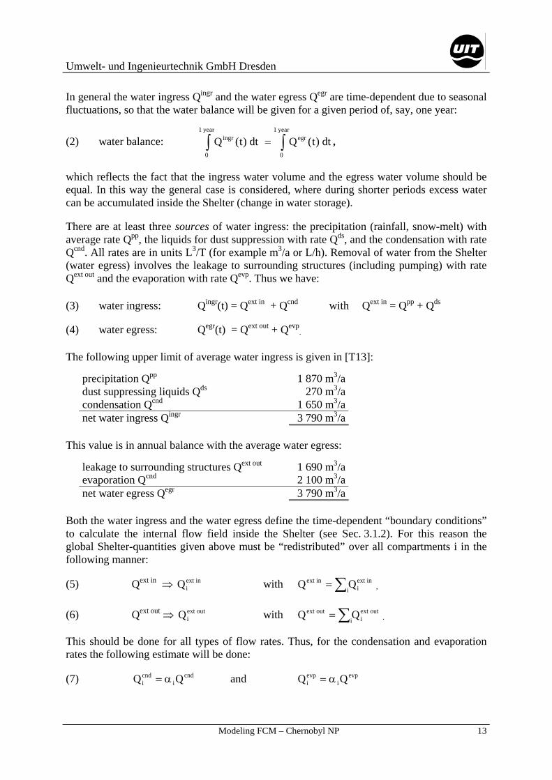
In general the water ingress Qingr and the water egress Qegr are time-dependent due to seasonal fluctuations, so that the water balance will be given for a given period of, say, one year:
(2) water balance: ∫∫ =year1
0
egryear1
0
ingr dt)t(Qdt)t(Q ,
which reflects the fact that the ingress water volume and the egress water volume should be equal. In this way the general case is considered, where during shorter periods excess water can be accumulated inside the Shelter (change in water storage). There are at least three sources of water ingress: the precipitation (rainfall, snow-melt) with average rate Qpp, the liquids for dust suppression with rate Qds, and the condensation with rate Qcnd. All rates are in units L3/T (for example m3/a or L/h). Removal of water from the Shelter (water egress) involves the leakage to surrounding structures (including pumping) with rate Qext out and the evaporation with rate Qevp. Thus we have:
(3) water ingress: Qingr(t) = Qext in + Qcnd with Qext in = Qpp + Qds
(4) water egress: Qegr(t) = Qext out + Qevp.
The following upper limit of average water ingress is given in [T13]:
precipitation Qpp 1 870 m3/adust suppressing liquids Qds 270 m3/acondensation Qcnd 1 650 m3/anet water ingress Qingr 3 790 m3/a
This value is in annual balance with the average water egress:
leakage to surrounding structures Qext out 1 690 m3/aevaporation Qcnd 2 100 m3/anet water egress Qegr 3 790 m3/a
Both the water ingress and the water egress define the time-dependent “boundary conditions” to calculate the internal flow field inside the Shelter (see Sec. 3.1.2). For this reason the global Shelter-quantities given above must be “redistributed” over all compartments i in the following manner:
(5) Qext in ⇒ inextiQ with ∑= i
inexti
inext QQ ,
(6) Qext out ⇒ outextiQ with ∑= i
outexti
outext QQ .
This should be done for all types of flow rates. Thus, for the condensation and evaporation rates the following estimate will be done:
(7) cndi
cndi QQ α= and evp
ievpi QQ α=
Umwelt- und Ingenieurtechnik GmbH Dresden
14 Modeling FCM – Chernobyl NPP
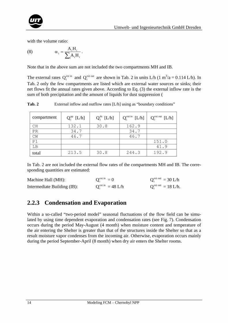
with the volume ratio:
(8) ∑
=αi ii
iii HA
HA .
Note that in the above sum are not included the two compartments MH and IB. The external rates inext
iQ and outextiQ are shown in Tab. 2 in units L/h (1 m3/a = 0.114 L/h). In
Tab. 2 only the few compartments are listed which are external water sources or sinks; their net flows fit the annual rates given above. According to Eq. (3) the external inflow rate is the sum of both precipitation and the amount of liquids for dust suppression ( Tab. 2 External inflow and outflow rates [L/h] using as “boundary conditions”
compartment ppiQ [L/h] ds
iQ [L/h] inextiQ [L/h] outext
iQ [L/h]
CH 132.1 30.8 162.9 PR 34.7 34.7 CW 46.7 46.7 P1 151.0 LB 41.9 total 213.5 30.8 244.3 192.9
In Tab. 2 are not included the external flow rates of the compartments MH and IB. The corre-sponding quantities are estimated:
Machine Hall (MH): inextiQ = 0 outext
iQ = 30 L/h Intermediate Building (IB): inext
iQ = 48 L/h outextiQ = 18 L/h.
2.2.3 Condensation and Evaporation Within a so-called “two-period model” seasonal fluctuations of the flow field can be simu-lated by using time dependent evaporation and condensation rates (see Fig. 7). Condensation occurs during the period May-August (4 month) when moisture content and temperature of the air entering the Shelter is greater than that of the structures inside the Shelter so that as a result moisture vapor condenses from the incoming air. Otherwise, evaporation occurs mainly during the period September-April (8 month) when dry air enters the Shelter rooms.

Umwelt- und Ingenieurtechnik GmbH Dresden
Modeling FCM – Chernobyl NP 15
Fig. 7 Example for the time-dependence of the condensation and evaporation rates (seasonal fluctuations)
2.2.4 Internal Water Flow The water flow through adjacent compartments represents the internal flow field. Its time-dependence is determined by the “boundary conditions”: the external flow rates including condensation and evaporation. In principle there are two ways for using these “boundary con-ditions” to calculate the internal flow field:
Case 1: The external inflow rate will be given (not outflow rates). The model determines the time-dependent outext
iQ under the condition that the water volume inside all compartments is zero or constant, Vi(t) = const (no change in water storage). The time-dependence results from seasonal fluctuations of the condensation and evaporation rates – see Sec. 2.2.3. Case 2: The external inflow and outflow rates will be given. The model calculates then the water storage fluctuations Vi(t) ≠ 0 due to accumulation of excess water in the compartments. In other words, the water ingress in the upper compartments results in water pools at the lower Shelter levels. The purpose of this section is to quantify the hydraulic couplings between adjacent compart-ments. This task is solved by using so-called splitting or distribution coefficients kij to “navi-gate” the water flow inside the Shelter. [A description based on conductivity’s and Darcy-law is in principle possible but for this problem not adequate since the Shelter represents a hetero-geneous system of porous media and fracture networks.] The splitting coefficient kij (model input) is defined as the ratio of the transferred water amount from compartment i→j to the water amount in compartment i. Its value is therefore smaller or equal to one, kij ≤ 1. Two compartments are isolated from each other if kij = 0; on the other hand, kij = 1 describes total discharge.
0
100
200
300
400
500
600
700
Sep 97 Jan 98 Apr 98 Jul 98 Nov 98 Feb 99 Mai 99 Aug 99 Dez 99 Mrz 00
cond
ansa
tion
/ eva
pora
tion
rate
s [L/
h] Q_cnd Q_evp
Umwelt- und Ingenieurtechnik GmbH Dresden
16 Modeling FCM – Chernobyl NPP
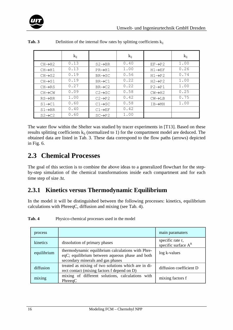
Tab. 3 Definition of the internal flow rates by splitting coefficients kij
kij kij kij
CH→H2 0.13 S2→BR 0.40 EF→P2 1.00
CH→H1 0.13 PR→H1 1.00 H1→EF 0.26
CH→S2 0.19 BR→SC 0.56 H1→P2 0.74
CH→S1 0.19 BR→C1 0.22 H2→P2 1.00
CH→RS 0.27 BR→C2 0.22 P2→P1 1.00
CH→CW 0.09 C2→SC 0.58 CW→H2 0.25
RS→BR 1.00 C2→P2 0.42 CW→LB 0.75
S1→C1 0.60 C1→SC 0.58 IB→MH 1.00
S1→BR 0.40 C1→EF 0.42
S2→C2 0.60 SC→P2 1.00
The water flow within the Shelter was studied by tracer experiments in [T13]. Based on these results splitting coefficients kij (normalized to 1) for the compartment model are deduced. The obtained data are listed in Tab. 3. These data correspond to the flow paths (arrows) depicted in Fig. 6. 2.3 Chemical Processes The goal of this section is to combine the above ideas to a generalized flowchart for the step-by-step simulation of the chemical transformations inside each compartment and for each time step of size ∆t. 2.3.1 Kinetics versus Thermodynamic Equilibrium In the model it will be distinguished between the following processes: kinetics, equilibrium calculations with PhreeqC, diffusion and mixing (see Tab. 4).
Tab. 4 Physico-chemical processes used in the model
process main paramaters
kinetics dissolution of primary phases specific rate r, specific surface AR
equilibrium thermodynamic equilibrium calculations with Phre-eqC; equilibrium between aqueous phase and both secondary minerals and gas phases
log k-values
diffusion treated as mixing of two solutions which are in di-rect contact (mixing factors f depend on D) diffusion coefficient D
mixing mixing of different solutions, calculations with PhreeqC mixing factors f

Umwelt- und Ingenieurtechnik GmbH Dresden
Modeling FCM – Chernobyl NP 17
The interrelations of typical physico-chemical processes is demonstrated in Fig. 8:
• the dissolution of the primary phase (as a kinetic process) which is in contact with the stagnant water surrounding the phase as a thin film,
• the precipitation of secondary phases as a result of equilibrium calculations (with Phre-eqC),
• the diffusion process between the stagnant water and mobile water, • the mixing of the mobile water phase with incoming waters from other compartments
and/or the outside. In each time-step a quasi-equilibrium is assumed. The appropriate intensive parameters such as pH, and redox potential Eh are calculated with PhreeqC which includes:
• ion speciatiation and charge balance, • activity coefficients from Davies or extended Debye-Hückel equation,, • aqueous complexation, • redox reactions, • equilibrium with solid and gas phases, • ion-exchange, • sorption and surface-complexation.
The obtained intensive parameters (pH, Eh) influence the stability of phases and, in this way, the dissolution kinetics.
Fig. 8 Scheme of typical processes within one compartment: kinetics (kin), equilibrium proc-esses (eq) and diffusion (diff)
The most important parameter for equilibrium calculations is the so-called equilibrium con-stant (log-k value) for each reaction which enters the mass-action equation. These data are stored in thermodynamic libraries (ASCII files). Data for Shelter-specific phases which are not included in common libraries (wateq4f.dat, etc.) will be deduced from GEM-calculations with help of Selektor-A code.
kin
outflow
inflow
primary phases
mobile water
secondary phases
stagnant water
diff
eq

Umwelt- und Ingenieurtechnik GmbH Dresden
18 Modeling FCM – Chernobyl NPP
Formally, the dissolution and precipitation processes can be described either as an equilib-rium approach (using PhreeqC) or as a kinetic approach. The advantage of the thermody-namic equilibrium approach is that for each phase only one parameter (log-k value) is neces-sary whereas the kinetic approach needs several parameters (rate constants r, hydrologic pa-rameters like the reactive surface, etc.) which are difficult to measure. However, a major defi-ciency with equilibrium models is that minerals and other reactants often do not react to equi-librium in the time frame of a model period ∆t. A kinetic approach is then required. For this reason, both approaches will be used in the dynamical compartment model as shown in Tab. 4.
Mathematically, the dynamics of phase transformations depicted in Fig. 8 will be described by a system of differential equations in Sec. 3.4.1. 2.3.2 Components of Shelter Waters The chemical composition of a solution (Shelter water) is defined by the following parame-ters:
intensive parameters: pH, Eh, T, major constituents (> 5 mg/L): Ca, Mg, Na, K, Si, C, S, Cl, P, minor constituents (< 5 mg/L): U, Al, Fe, trace constituents: Sr, Cs.
The water composition is determined by typical processes or several sources (see Tab. 5):
• equilibrium to air (O2, CO2), • dissolution of primary solid phases (CM, DM, CF, LFCM, HP) which produces the sol-
utes U, Ca, K, Na, Mg, Si, and other elements.
The thermodynamic equilibrium with secondary minerals serves as rate limiting processes: it acts as a “sink term” if supersaturation occurs.
Tab. 5 Origin and source of the Shelter-water components
component origin or source
O contact with air C contact with air; dumping material dolomite Ca phase CHS (and Arg-Str) Mg phase hydrotalcite Na dumping material Na3PO4 K phase: ? (or “noise” KCl) Si phase CHS; (and LFCM dissolution) Al phase hydrotalcite Fe corrosion phase: hydrogoethite, hydromagnetite Cl phase in serpentine concrete ? S phase Arg-Str (gypsum ?) P dumping materials: Na3PO4

Umwelt- und Ingenieurtechnik GmbH Dresden
Modeling FCM – Chernobyl NP 19
U dissolution kinetics of FCM The sources of Fe are mainly the corrosion products of the construction material “steel”: hy-drogoethite, hydromagnite. The sources of Na and P is the dumping material Na3PO4 thrown from helicopters to smoother the reactor fire during the “Active Phase Accident Management Actions” [Sich94]. The list of the equilibrium phases acting as sources or as sinks is given in Sec. 4.2.1. It should be noted, that there are some problems to identify exactly the sources of K, S and Cl inside the Shelter. If these elements are underestimated in the actual calculations a so-called initial background composition will be generated by adding salts such as NaCl, Na2SO4 and/or KCl. The amount of these chemicals will be adjusted to the observed data. The trace constituents Sr and Cs are treated as so-called non-reactive tracer elements which will be dissolved from FCM and transported inside the Shelter. Tracer elements are not in-cluded into thermodynamic equilibrium calculations with PhreeqC. 2.3.3 Chemical Transformations inside a Compartment Collecting all facts discussed above the main procedure for calculating the solid-aqueous in-teraction within one compartment can be defined. The general scheme is given in Fig. 9. It is the same for each compartment and contains all processes which subsequently will be calcu-lated (principle of superposition). However, in the first model version only the dominant proc-esses should be considered. The general procedure is decomposed into six steps. After each step a typical solution (of the mobile aqueous phase) will be calculated which is numbered by 1 to 6. mobile aqueous phases: solution 1: solution after mixing of inflow waters from other compartments; equilibrium
with air (gas phases: CO2 and O2),
solution 2: solution after diffusion exchange with stagnant water phase from cement pores (solution a),
solution 3: solution after diffusion exchange with stagnant water phase from unaltered nuclear fuel pores (solution b),
solution 4: solution after diffusion exchange with stagnant water phase from lava pores (solution c),
solution 5: solution subsequent to kinetic dissolution of hot particles, solution 6: solution after evaporation and equilibrium with secondary uranium minerals
SUM 2; (evaporation lead to increases in concentrations which are proportional to the amount of water that evaporates)
Solution 6 serves as the input water for adjacent compartments.

Umwelt- und Ingenieurtechnik GmbH Dresden
20 Modeling FCM – Chernobyl NPP
Fig. 9 General flowchart of chemical processes within one compartment which are per-
formed at each time step of size ∆t
In intermediate steps the pore solutions are calculated: stagnant aqueous phases (pore solutions):
solution a: cement pore water which is in equilibrium with cement phases; the redox po-tential of this solution will be fixed to a realistic value (Eh ≈ -80 to –120 mV);
solution b: pore water or thin film of water surrounding the unaltered nuclear fuel frag-ments; the composition of this water is determined from:
• dissolution kinetics of UO2, • equilibrium with secondary uranium phases SUM 1, • diffusion contact with mobile solution 2,
b
kin
kin
kin
diff
diff
diff
evaporation
inflow from othercompartments
outflow to othercompartments
CF
LFCM
CM
SUM 1
SUM 1
SUM 2
HP
a
3
2
4
5
c
air
6
1
Umwelt- und Ingenieurtechnik GmbH Dresden
Modeling FCM – Chernobyl NP 21
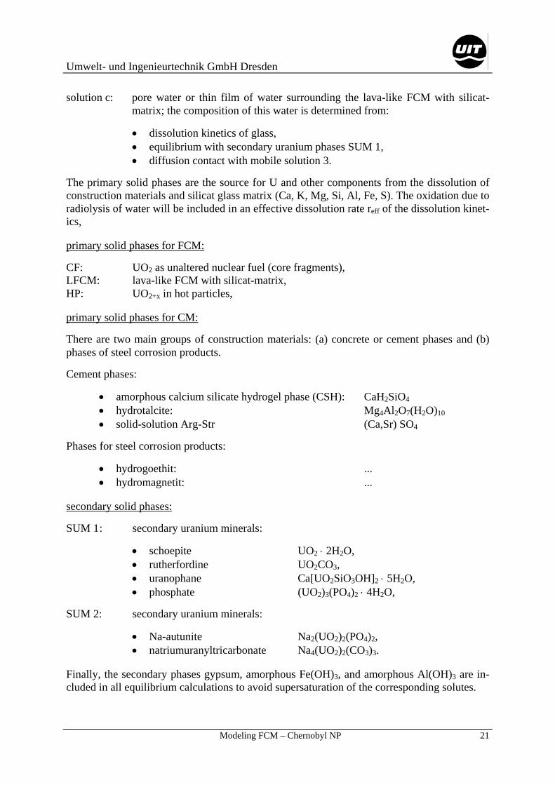
solution c: pore water or thin film of water surrounding the lava-like FCM with silicat-matrix; the composition of this water is determined from:
• dissolution kinetics of glass, • equilibrium with secondary uranium phases SUM 1, • diffusion contact with mobile solution 3.
The primary solid phases are the source for U and other components from the dissolution of construction materials and silicat glass matrix (Ca, K, Mg, Si, Al, Fe, S). The oxidation due to radiolysis of water will be included in an effective dissolution rate reff of the dissolution kinet-ics, primary solid phases for FCM:
CF: UO2 as unaltered nuclear fuel (core fragments), LFCM: lava-like FCM with silicat-matrix, HP: UO2+x in hot particles, primary solid phases for CM:
There are two main groups of construction materials: (a) concrete or cement phases and (b) phases of steel corrosion products.
Cement phases:
• amorphous calcium silicate hydrogel phase (CSH): CaH2SiO4 • hydrotalcite: Mg4Al2O7(H2O)10 • solid-solution Arg-Str (Ca,Sr) SO4
Phases for steel corrosion products:
• hydrogoethit: ... • hydromagnetit: ...
secondary solid phases:
SUM 1 : secondary uranium minerals:
• schoepite UO2 ⋅ 2H2O, • rutherfordine UO2CO3, • uranophane Ca[UO2SiO3OH]2 ⋅ 5H2O, • phosphate (UO2)3(PO4)2 ⋅ 4H2O,
SUM 2: secondary uranium minerals:
• Na-autunite Na2(UO2)2(PO4)2, • natriumuranyltricarbonate Na4(UO2)2(CO3)3.
Finally, the secondary phases gypsum, amorphous Fe(OH)3, and amorphous Al(OH)3 are in-cluded in all equilibrium calculations to avoid supersaturation of the corresponding solutes.

Umwelt- und Ingenieurtechnik GmbH Dresden
22 Modeling FCM – Chernobyl NPP
2.3.4 Relations between Kinetic Parameters for FCM Assuming zero-order kinetics there are three specific rates [mol⋅m-2⋅s-1] for uranium:
rCF for dissolution of unaltered fuel UO2 from CF, rLFCM for dissolution of uranium from LFCM, rHP for dissolution of UO2+x from HP,
and for silicium
rSi for dissolution of Si from LFCM. Obviously, from observations the following relations between dissolution rates can be qualita-tively deduced:
rHP >> rCF and rHP >> rLFCM ,
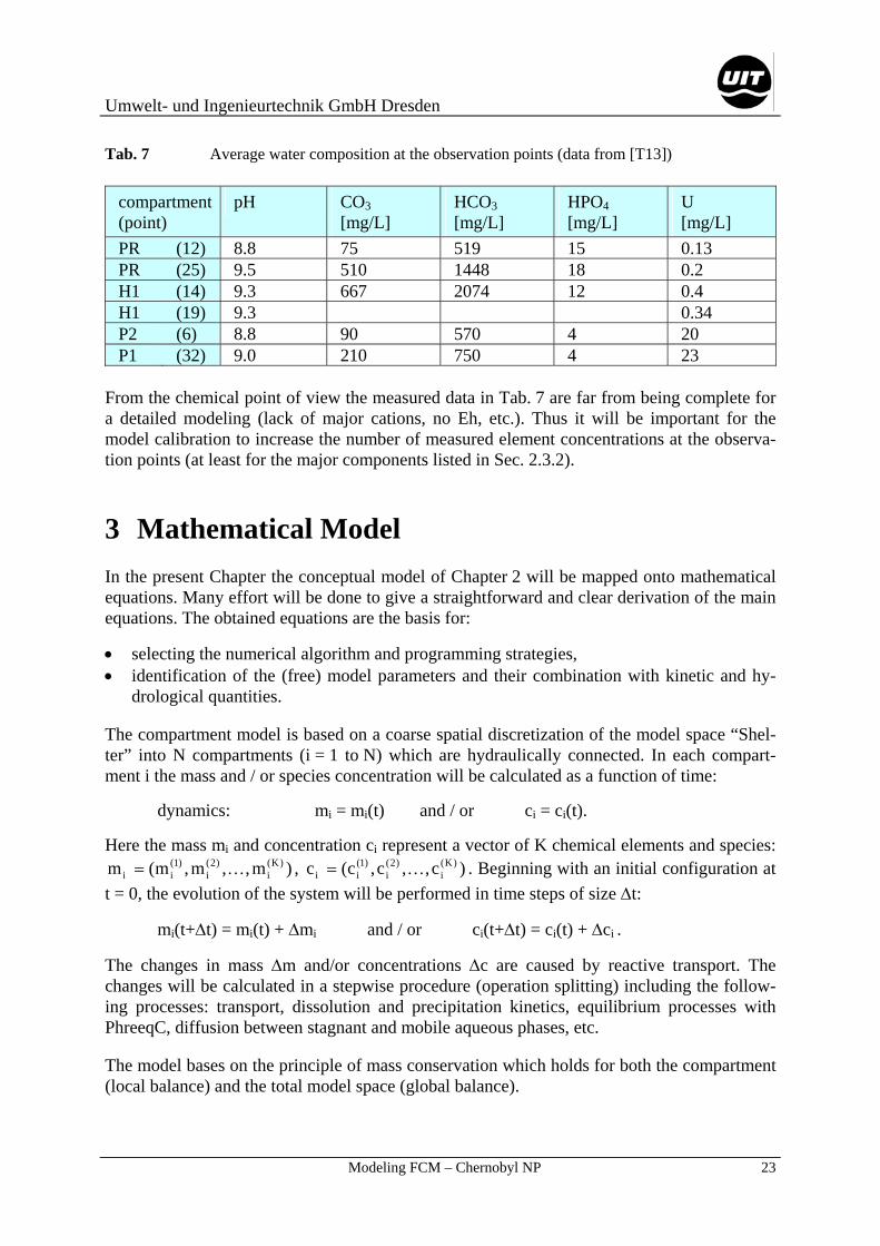
which reflect the fact that the dominant dissolution process for U is the dissolution of (high-oxidized) nuclear fuel powder – HP. Therefore, in a first model version the uranium content in the Shelter water will be described by the dissolution of hot particles (and neglecting the LFCM and CF dissolution processes, rCF = 0, rLFCM = 0). Typical values for rHP will be pre-sented in Sec. 4.2.3. 2.3.5 Example: Water Percolation through the Shelter Based on existing sample points a chain of compartments can be constructed to investigate the percolation of water downstream inside the Shelter (see Fig. 2): PR ⇒ H1 ⇒ P2 ⇒ P1. The location of the observation points inside the Shelter are given in Tab. 6. The correspond-ing average water compositions are listed in Tab. 7. Along the chain from the upper to the lower levels the uranium content in the water increases due to interactions with FCM. The rapid increasing of U from about 0.4 mg/L (in compartment H1) to 20 mg/L (in compartment P2) is caused by the fact that P2 obtains additional inflows from other compartments such as EF, SC and H2 (see Fig. 2). It is the object of the compartment model to combine all flow paths in the calculation while the above chain represents only a fragment of the flow pattern.
Tab. 6 Location of observation points inside the Shelter
point compartment room axis row level [m] 12 PR 402/3 49-50 D – E 24.0 25 PR 402/3 49 D 18.5 14 H1 406/2 43-44 Zh – I 12.5 19 H1 219/2 42-43 M – N 6.0 6 P2 012/16 48-49 E – Zh 2.2 32 P1 012/7 47-48 E – Zh -0.65
Umwelt- und Ingenieurtechnik GmbH Dresden
Modeling FCM – Chernobyl NP 23
Tab. 7 Average water composition at the observation points (data from [T13])
compartment (point)
pH CO3 [mg/L]
HCO3 [mg/L]
HPO4 [mg/L]
U [mg/L]
PR (12) 8.8 75 519 15 0.13 PR (25) 9.5 510 1448 18 0.2 H1 (14) 9.3 667 2074 12 0.4 H1 (19) 9.3 0.34 P2 (6) 8.8 90 570 4 20 P1 (32) 9.0 210 750 4 23
From the chemical point of view the measured data in Tab. 7 are far from being complete for a detailed modeling (lack of major cations, no Eh, etc.). Thus it will be important for the model calibration to increase the number of measured element concentrations at the observa-tion points (at least for the major components listed in Sec. 2.3.2).
3 Mathematical Model In the present Chapter the conceptual model of Chapter 2 will be mapped onto mathematical equations. Many effort will be done to give a straightforward and clear derivation of the main equations. The obtained equations are the basis for:
• selecting the numerical algorithm and programming strategies, • identification of the (free) model parameters and their combination with kinetic and hy-
drological quantities. The compartment model is based on a coarse spatial discretization of the model space “Shel-ter” into N compartments (i = 1 to N) which are hydraulically connected. In each compart-ment i the mass and / or species concentration will be calculated as a function of time:
dynamics: mi = mi(t) and / or ci = ci(t).
Here the mass mi and concentration ci represent a vector of K chemical elements and species: )m,,m,m(m )K(
i)2(
i)1(
ii K= , )c,,c,c(c )K(i
)2(i
)1(ii K= . Beginning with an initial configuration at
t = 0, the evolution of the system will be performed in time steps of size ∆t:
mi(t+∆t) = mi(t) + ∆mi and / or ci(t+∆t) = ci(t) + ∆ci .
The changes in mass ∆m and/or concentrations ∆c are caused by reactive transport. The changes will be calculated in a stepwise procedure (operation splitting) including the follow-ing processes: transport, dissolution and precipitation kinetics, equilibrium processes with PhreeqC, diffusion between stagnant and mobile aqueous phases, etc. The model bases on the principle of mass conservation which holds for both the compartment (local balance) and the total model space (global balance).

Umwelt- und Ingenieurtechnik GmbH Dresden
24 Modeling FCM – Chernobyl NPP
3.1 Basic Equations In this section both the advection-reaction equation and the flow equation for the compart-ment model are derived from the principle of mass conservation. Due to the conceptual dif-ference between the compartment model and the transport models in hydrogeology [DS98] the obtained equations differ in several respects from the common used equations in hydro-geology. The derived equations are the basis for the numerical model in Sec. 3.2. 3.1.1 Advection-Reaction Equation Conservation of mass for a chemical that is transported yields:
change in mass storage with time = mass inflow rate – mass outflow rate + mass production rate
in units of mass per unit of time (MT-1). This statement applies to a domain of any size, that is, for one compartment as well as for the whole system. Let us now consider the (mobile) aqueous phase in compartment i with mass ii
aqi Vcm = . The change in mass is then given by
the
(9) advection-reaction equation: iRi
adv
iaqi RV
dtdm
dtdm
+⎟⎟⎠
⎞⎜⎜⎝
⎛= ,
where the first term corresponds to the advection. The second term describes the fluid sink/source with Ri = Ri(ci) as the reaction rate in units (ML-3T-1) and R
iV as the correspond-ing reaction volume (L3). The sink/source term results from interactions with other subsys-tems (stagnant water domain and/or solid phases) and will be specified in Sec. 3.3. The mass transport due to advection can be expressed by the
(10) advection equation: [ ] 0evpi
cndi
N
0jijijij
adv
i c)QQ(cQcQdt
dm−+−=⎟⎟
⎠
⎞⎜⎜⎝
⎛∑=
→→ ,
where
aqim = ciVi element mass in mobile water of compartment i M
Vi volume of mobile water in compartment i L3 ci element concentration in mobile water of compartment i ML-3 c0 element concentration in pure water (H2O) ML-3 c0 element concentration of external inflow water (rain water) ML-3
jiQ → hydraulic flow rate from compartment i to compartment j L3T-1 cndiQ condensation rate in compartment i L3T-1 evpiQ evaporation rate in compartment i L3T-1.
Umwelt- und Ingenieurtechnik GmbH Dresden
Modeling FCM – Chernobyl NP 25
Note, that all quantities are functions of time: c = c(t), Q = Q(t), V = V(t). The sum over j in Eq. (10) also includes the coupling to the environment or “outside region” of the Shelter (car-rying the subscript 0):
Q0→i = inextiQ hydraulic inflow rate from outside to compartment i L3T-1
Qi→0 = outextiQ hydraulic outflow rate from compartment i to outside L3T-1.
In this way, the net inflow/outflow rate in compartment i is the sum of two contributions: the outside inflow/outflow (external coupling) and the inflow/outflow from other compartments (internal coupling):
(11) ∑=
→→ +=+=N
1j
ininti
inextiiji0
ini QQQQQ ,
(12) ∑=
→→ +=+=N
1j
outinti
outextiji0i
outi QQQQQ .
Obviously, external inflow appears in the upper level compartments, whereas the external outflow is in the lower level compartments of the Shelter. The corresponding external flow rates are specified in Tab. 2. The distinction between external and internal flow is important since the external flow determines the internal flow field as a kind of time-dependent “bound-ary condition”. 3.1.2 Flow Equation and Flow Field Mathematically, the change in mass consists of two terms according to the product rule of a derivative:
(13) mi = Vi ci ⇒ dt
dcVdt
dVcdt
dm ii
ii
i += .
Using this product rule one obtains for the left-hand side of Eq. (9) the expression
(14) [ ] [ ] iRi
0evpi
cndi
N
0jijijij
ii
ii RVcQQcQcQ
dtdcV
dtdVc +−+−=+ ∑
=→→ .
For constant concentrations such as pure water, ci = c0 = [H2O], and in absence of reactions (Ri = 0), the above expression reduces to the
(15) flow equation: [ ] ( )evpi
cndi
N
0jjiij
i QQQQdt
dV−+−= ∑
=→→ ,
which is determined solely by the flow rates Q. The flow equation is a special case of the ad-vection equation (10) applied for pure water transport. If the water volume in all compartments is not changed, dVi/dt = 0 for all i, we have Vi(t) = const = Vi(0) and stationarity holds,

Umwelt- und Ingenieurtechnik GmbH Dresden
26 Modeling FCM – Chernobyl NPP
(16) steady state: [ ] ( ) 0QQQQ evpi
cndi
N
0jjiij =−+−∑
=→→ .
For numerical purposes it is useful to rewrite the flow equation into the expanded form (for small ∆t):
(17) ( ) tQQQQ)t(V)tt(V evpi
cndi
outi
iniii ∆−+−+=∆+ ,
where the definitions in Eqs. (11) and (12) are incorporated. Note that for finite ∆t Eq. (17) is an approximation of the flow equation (15) which becomes exact if either ∆t → 0 or all Q’s are time-independent. Formally, Eq. (17) is obtained by integration of the flow equation from t to t+∆t supposing that all Q’s are constant within the interval ∆t. In practice the size of ∆t depends on the time scale of Q-changes. Calculation of the Flow Field. The internal flow field as a function of time is determined solely by the external flow rates including the time-dependent condensation and evaporation rates (time-dependent “boundary conditions”). The flow field will be calculated iteratively for every time step. In general, the following options are possible to describe the compartment-by-compartment flow:
• Qi→j = Lij (hi–hj) as a function of the hydraulic gradient ∆h (Darcy-law like approach to flow in porous media or the flow in open drifts or raises); as input effective conductivities Lij in units L2T-1 are used,
• Qi→j calculated by so-called splitting coefficients kij (input values with dimension 1), • flow-field calculation as a combination of both methods (vertical flow by splitting coeffi-
cients; horizontal flow by conductivities).
To calculate the flow field in the Shelter, splitting coefficients rather than conductivities will be used. The splitting coefficients kij can be estimated from the ratio of the interface area of two adjacent compartments or from flow paths information’s taken from tracer experiments, respectively. The flow rate between compartment i and j is then given by (18) ( )evp
icndi
inintiijji QQQkQ −+=→ with 1k
jij =∑ .
Splitting coefficients for the Shelter system are listed in Tab. 3. [Accumulation of excess wa-ter occurs in compartment i if the condition 1k
jij <∑ holds, respectively.]
3.1.3 Linkage between Flow and Transport The changes in concentration, dci/dt, are obtained directly from Eq. (14) after replacing the term dVi/dt by the flow equation (15). This yields the linkage between flow and transport in one expression:
(19) ( ) ( ) iRii
0evpi
cndi
N
0jijij
ii RVccQQ)cc(Q
dtdcV +−−+−= ∑
=→ .
Umwelt- und Ingenieurtechnik GmbH Dresden
Modeling FCM – Chernobyl NP 27
It is worth nothing that in this equation the outflow rates Qi→j are disappeared. For further purposes Eq. (19) will be written in the expanded form (for small ∆t):
(20) ( ) ( ) tRVtccQQt)cc(QcV)tt(cV iRii
0evpi
cndi
N
0jijijiiii ∆+∆−−+∆−+=∆+ ∑
=→ .
The concentrations on the right-hand side are given at time t. Equation (20) together with Eq. (17) are the main formulas for the further numerical treatment in Sec. 3.2. 3.2 Numerical Model Based on the above equations the numerical model can be defined. Thereby, the calculation of mass transport and mass transformations as a function of time will be performed iteratively for each compartment i and for each time step with steps of size ∆t:
(21) )tt(c)tt(V)tt(m)t(m iiii ∆+∆+=∆+⇒ .
This task is solved within a two-step algorithm which separates between flow and reactive transport:
• first step: )tt(V)t(V ii ∆+⇒ and )tt(Q)t(Q jiji ∆+⇒ →→ for i,j ≥ 1,
• second step: )tt(c)t(c ii ∆+⇒
using the following “start values”:
iV (t=0) and ic (t=0) (initial condition), )t(Q inext
i and )t(Q outexti (“boundary condition”).
The time-dependent “boundary conditions” also contain the condensation and evaporation rates. In the first step, the water volume and the internal flow field (including all Qi→j for i,j ≥ 1) are calculated for time t+∆t using Eq. (17) – the flow equation in the expanded form. Based on the obtained quantities Vi and Qi→j, in a second step the concentrations are calculated by Eq. (20). The second step is performed using the “mixing operation” of a thermodynamic model (equilibration calculation with PhreeqC). However, to calculate ci(t+∆t) by Eq. (20) two cases should be distinguished:
• case 1: Vi > 0 (flow through not-empty compartments), • case 2: Vi = 0 (flow through empty compartments).
For example, case 1 describes the situation for the low-lying compartments located near the earth surface in which water is accumulated in pools. On the other hand, case 2 describes the common situation for the upper-level compartments where water flows through “empty com-
Umwelt- und Ingenieurtechnik GmbH Dresden
28 Modeling FCM – Chernobyl NPP
partments” without accumulation of excess water. To avoid zero volumes in Eq. (20), the fol-lowing assumption should be made in case 2: (22) t)QQQ(V evp
icndi
inii ∆−+= if Vi = 0,
which is indeed zero if ∆t → 0. In this way, for both cases the following “mixing formula” is obtained from Eq. (20):
(23) tRVVcfc)f1()tt(c i
i
Ri
N
0jjijiii ∆++−=∆+ ∑
=
with the mixing factors:
(24) tV
Qf
i
ijij ∆= → and
(25) ( )∑
=
∆−+
=∆−
+=N
0j i
evpi
cndi
ini
i
evpi
cndi
iji tV
QQQtV
QQff
(which holds for concentrations different from H2O, i. e., for ci ≠ c0). In case 2 the above mix-ing equation further reduces to:
(26) evpi
cndi
ini
iRi
N
0jjiji QQQ
RVcf)tt(c−+
+=∆+ ∑=
.
Whereas Eq. (23) is appropriate for compartments containing water pools with volume Vi = const (stationary pool) or Vi = Vi(t) (temporary pools), Eq. (26) holds for compartments without water pools. 3.3 Sink/Source Term In general, the source term in Eq. (9) can be used to describe any kinetic process or non-advective mass exchange with other subsystems. In Sec. 3.3.1 we will consider both dissolu-tion and diffusion processes and discuss the structure of the corresponding rate equations. In Sec. 3.3.3 the dissolution/precipitation processes are described by an equilibrium approach.
3.3.1 Diffusion and Dissolution Processes The overall reaction rate Ri and reaction volume R
iV in the advection-reaction equation (9) should be replaced by S
iR , SiV in case of dissolution kinetics or by D
iR , DiV in case of diffu-
sion processes, respectively, for which the following expressions hold:
(27) dissolution: γ
⎟⎟⎠
⎞⎜⎜⎝
⎛=
)0(m)t(m
arR s
i
si
S
Si with ⎟⎟
⎠
⎞⎜⎜⎝
⎛= S
i
Si
S AV
a ,

Umwelt- und Ingenieurtechnik GmbH Dresden
Modeling FCM – Chernobyl NP 29
(28) diffusion: ( )ii2D
Di cc~
aDR −= with ⎟⎟
⎠
⎞⎜⎜⎝
⎛= D
i
Di
D AV
a .
The quantities are:
SiR overall reaction rate for dissolution ML-3T-1
DiR diffusion rate ML-3T-1
r specific rate for dissolution ML-2T-1 D diffusion coefficient L2T-1
SiV “reactive” water volume in contact with the solid L3 DiV volume of “diffusion layer” (between stagnant and mobile water) L3 SiA (initial) surface area of the solid which is in water contact L2 DiA surface of “diffusion layer” (between stagnant and mobile water) L2
ci concentration in the mobile aqueous phase ML-3 ic~ concentration in the stagnant aqueous phase ML-3
sim (t) moles of solid at given time t in compartment i M.
The last factor in the expression for S
iR in Eq. (27) is named demolition factor. It accounts for changes in the size during dissolution and also for selective dissolution and aging of the solid. For uniformly dissolving spheres and cubes γ = 2/3. For large mass supply the demolition factor in round brackets can be set equal to 1. In both cases the overall reaction rate Ri is decomposed into a “geometrical factor”, aS and aD, and a material-specific constant: the reaction rate r or the diffusion coefficient D. It should be noted, that whereas D
iA , DiV , S
iA , and SiV are depend on (the mass deposit of) compartment i
the parameters aD and aS are independent of i. The stagnant water volume which is in direct contact with the solid matrix can be approxi-mated by the volumetric water content θ (moisture content in units L3/L3) and the volume of the solid, s
si /m ρ :
(29) s
sis
imVρ
θ= ,
where ρs represents the bulk density of the solid in units ML-3. If the pores of the matrix are totally filled with water the quantity θ becomes equal to the porosity n, that is θ ≤ n. Thus, for saturated media θ should be replaced by n in the above equation. Another important parameter is the specific surface area s
iSis m/AA = in m2/g (or m2/100 g
solid medium), which can be measured by BET method. Note, that the specific quantity As is independent of the compartment number i. In this way, the above parameter aS can be ex-pressed by

Umwelt- und Ingenieurtechnik GmbH Dresden
30 Modeling FCM – Chernobyl NPP
(30) ss
S Aa
ρθ
= .
Once more it reflects the fact that aS is a specific quantity which is independent of the com-partment number i. 3.3.2 First-Order Kinetics The specific rate r for a given substance can be a constant (zero-order kinetics) or a linear function of the concentration (first-order kinetics). As a special kind of first-order kinetics the following rate is often applied [PA99]:
(31) ⎥⎥⎦
⎤
⎢⎢⎣
⎡⎟⎠⎞
⎜⎝⎛−=
σ
kIAP1rr 0 ,
where r0 is an empirical constant and IAP/k is the saturation ratio. This rate equation can be derived from transition-state theory (TST), where the coefficient σ is related to the stoichiometry of the reaction when an activated complex is formed (often σ = 1). An advan-tage of this expression is that it applies for both supersaturation and undersaturation, and the rate is zero at equilibrium. The rate is constant over a large domain whenever the geochemical reaction is far from equilibrium (IAP/k > 0.1), and the rate approaches zero when IAP/k ap-proaches 1.0 (equilibrium). The diffusion process in Eq. (28) is treated as a kind of first-order kinetics which depends on the concentration difference between the two adjacent aqueous phases. Directly measured values for diffusion of ions in aqueous solutions are in the order D ≈ 10-5 cm2/s [AP93]. A model assumption is that the diffusion coefficient D is approximately equal for all species. 3.3.3 Water-Solid Equilibrium As was already discussed, the fast dissolution/precipitation processes can be described by using thermodynamic equilibrium models if the appropriate dissolution constant (log-k value) is known. Within the dynamical compartment model this method will be used to describe the interaction of stagnant waters with minerals, respectively. At each time step a so-called quasi-equilibrium is assumed. Equilibrium processes – which naturally does not contain the time-parameter t – can formally be mapped onto a dynamical description with sink/source terms like in Eq. (9). This is done by using Dirac’s delta-function, δ(t-teq), for the overall “reaction rate”: (32) equilibrium: ( ) )tt(ccR eqi
eqeqi −δ−= ,
where teq denotes the equilibration time, and ceq refers to the concentration of the species which is in equilibrium with the solid phase. Both quantities are related by ci(teq) = ceq. The equilibrium concentration ceq is independent of i; it will be obtained from PhreeqC-calculations.
Umwelt- und Ingenieurtechnik GmbH Dresden
Modeling FCM – Chernobyl NP 31
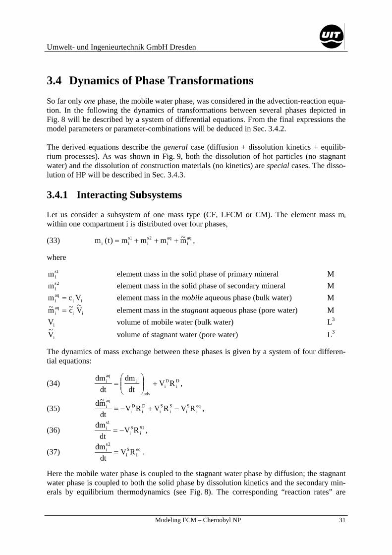
3.4 Dynamics of Phase Transformations So far only one phase, the mobile water phase, was considered in the advection-reaction equa-tion. In the following the dynamics of transformations between several phases depicted in Fig. 8 will be described by a system of differential equations. From the final expressions the model parameters or parameter-combinations will be deduced in Sec. 3.4.2. The derived equations describe the general case (diffusion + dissolution kinetics + equilib-rium processes). As was shown in Fig. 9, both the dissolution of hot particles (no stagnant water) and the dissolution of construction materials (no kinetics) are special cases. The disso-lution of HP will be described in Sec. 3.4.3. 3.4.1 Interacting Subsystems Let us consider a subsystem of one mass type (CF, LFCM or CM). The element mass mi within one compartment i is distributed over four phases,
(33) aqi
aqi
2si
1sii m~mmm)t(m +++= ,
where
1sim element mass in the solid phase of primary mineral M 2s
im element mass in the solid phase of secondary mineral M
iiaqi Vcm = element mass in the mobile aqueous phase (bulk water) M
iiaqi V~c~m~ = element mass in the stagnant aqueous phase (pore water) M
iV volume of mobile water (bulk water) L3
iV~ volume of stagnant water (pore water) L3
The dynamics of mass exchange between these phases is given by a system of four differen-tial equations:
(34) Di
Di
adv
iaqi RV
dtdm
dtdm
+⎟⎟⎠
⎞⎜⎜⎝
⎛= ,
(35) eqi
Si
Si
Si
Di
Di
aqi RVRVRV
dtm~d
−+−= ,
(36) 1Si
Si
1si RV
dtdm
−= ,
(37) eqi
Si
2si RV
dtdm
= .
Here the mobile water phase is coupled to the stagnant water phase by diffusion; the stagnant water phase is coupled to both the solid phase by dissolution kinetics and the secondary min-erals by equilibrium thermodynamics (see Fig. 8). The corresponding “reaction rates” are

Umwelt- und Ingenieurtechnik GmbH Dresden
32 Modeling FCM – Chernobyl NPP
taken from Eq. (27), Eq. (28) and Eq. (32). The advection term which describes the mass transport to other compartments and/or to the environment is expressed in Eq. (10). [To keep these equations transparent all stoichiometry coefficients are neglected in the notation, but they are included in calculations.] To reduce the number of free parameters the following assumption will be made: First, the space of the “diffusion layer” and “reactive dissolution volume” are identified as the volume of stagnant or pore water: i
Si
Di V~VV == . Second, the layer thickness or inverse specific sur-
face should be equal: aD = aS = a. Third, the precipitated secondary mineral does not influence the surface of the primary mineral. These assumptions lead to the following expressions:
(38) ( )ii2iadv
iaqi cc~
aDV~
dtdm
dtdm
−+⎟⎟⎠
⎞⎜⎜⎝
⎛= ,
(39) ( ) ( ) )tt(ccV~)0(m)t(m
arV~cc~
aDV~
dtm~d eq
ieq
i1si
1si
iii2i
aqi −δ−+⎟⎟
⎠
⎞⎜⎜⎝
⎛+−−=
γ
.
According to Eq. (29) the stagnant water volume can be expressed by the volumetric water content θ (or porosity n for saturated media) and the bulk density ρs. Using both Eq. (29) and Eq. (30) one gets the following parameter reduction:
(40) ssi
i AmaV~
= ,
where the parameters θ and ρs are cancelled. 3.4.2 Final Expressions and Model Parameters From Eq. (38) and Eq. (39) the following expressions for the concentrations in the mobile and stagnant aqueous phases are obtained
(41) ii
iN
0jjiji
i
iii c~g
VV~cfcg
VV~f1)tt(c ++⎟⎟
⎠
⎞⎜⎜⎝
⎛−−=∆+ ∑
=
(42) )cC()cC(C)tt(c~ eqi
eqiii −Θ−−=∆+
with the abbreviation
(43) tar gcc~)gf1(C iiii ∆++−−=
and the Heaviside step-function Θ(x) which results from integrating the Dirac’s delta-function to simulate the equilibrium processes:
(44) ⎩⎨⎧
<≥
=−Θaxax
for01
)ax( .

Umwelt- und Ingenieurtechnik GmbH Dresden
Modeling FCM – Chernobyl NP 33
The equilibrium concentration ceq depends on the chemical milieu of the pore water (includ-ing pH and Eh values) as well as on the dissolution constant (log-k value); ceq will be calcu-lated by PhreeqC. Let us focus to Eq. (41). It is a special form of Eq. (23) with the following abbreviation for the diffusion process
(45) taDg 2 ∆= .
Equation (41) consists of three terms, where the second term accounts for the coupling to other compartments and/or the boundaries (external waters), and the third term describes the coupling to the stagnant water phase. The final expressions in form of Eqs. (41) to (43) allow the extraction of the main model pa-rameters or combinations of them. Thereby, the most influencing factors affecting the trans-formation process of a mineral or solid phase define one parameter set. For example, a pa-rameter set is given by the following three quantities:
parameter set: D/a2 , r/a , and ./mV~ s1s
ii ρθ= 3.4.3 Special Case: Dissolution of Hot Particles The derived expressions become much more simpler in the special case of direct dissolution of hot particles in the mobile water (without diffusion processes from the stagnant water; see HP-dissolution in Fig. 9). Using the first-order kinetics for HP-dissolution reported in [Kp00] the system of differential equations for the aqueous and solid phases reduces to
(46) HPi
adv
iaqi m
dtdm
dtdm
κθ+⎟⎟⎠
⎞⎜⎜⎝
⎛= ,
(47) HPi
HPi m
dtdm
κθ−= .
Here, κ represents the first-order kinetic parameter in units T-1, which depends on both the oxidation state of the fuel particles and the pH of the solution [Kp00]. The factor θ accounts for the fact that only a fraction of the total material deposit located in a compartment gets con-tact with water. [In hydrogeology which considers the transport in porous media θ represents the moisture content (unsaturated case) or the porosity (saturated case).]
The iterative algorithm to calculate the time-dependent concentration and mass is then given by the simple expressions:
(48) ( ) HPi
i
N
0jjijiii m
Vtcfcf1)tt(c ∆κθ
++−=∆+ ∑=
(49) HPi
HPi m)t1()tt(m ∆κθ−=∆+ .

Umwelt- und Ingenieurtechnik GmbH Dresden
34 Modeling FCM – Chernobyl NPP
The parameterization of κ will be given in Sec. 4.2.3; a first application of these formulas to estimate the parameters is given in Sec. 4.3.2. 3.4.4 Local and Global Mass Balance The dynamical compartment model was derived from the principle of mass balance. This Sec-tion illustrates the local and global mass balance. The local mass balance holds for each com-partment i and can be obtained by the time derivative of Eq. (33) which leads to
(50) adv
iaqi
aqi
2si
1sii
dtdm
dtm~d
dtdm
dtdm
dtdm
dtdm
⎟⎟⎠
⎞⎜⎜⎝
⎛=+++= .
Here all source terms are cancelled. In other words, the net mass change in the compartment i is equal to the advective mass transport which exchanges mass with other compartments and/or with the environment.
Taking the sum over all compartments in Eq. (50) we get for the total model space “Shelter” the global mass balance
(51) [ ] [ ]∑∑∑===
−+−==N
1i
0evpi
cndi
N
1ii
outexti0
inexti
N
1i
i cQQcQcQdt
dmdtdm ,
which obviously does not include the internal couplings Qi→j for i, j ≥ 1. Note that in deriving Eq. (51) from Eq. (9) the following identity for the internal flows was used:
(52) [ ] 0cQcQ ijijij
N
1j
N
1i=− →→
==∑∑ .
For a “closed system” (no external couplings: Q0→i = Qi→j = 0) the above equation reduces to the stationary case dm/dt = 0 (perfect isolated Shelter).

Umwelt- und Ingenieurtechnik GmbH Dresden
Modeling FCM – Chernobyl NP 35
4 Data Preparation and Model Calibration
4.1 Input Data Structure The model calculations base on the following geometrical and hydraulic input data:
• geometrical data (size and location of compartments) see Tab. 1, • hydraulic data I (external flow rates) see Tab. 2, • hydraulic data II (splitting coefficients for internal flow field) see Tab. 3. The chemical input data are contained in two groups:
• thermodynamic data for equilibrium calculations (log-k values) contained in libraries, • kinetic data.
The ASCII-file named wateq4f.dat contains thermodynamic data for the aqueous species as well as the gas and mineral phases [BN91]. Data for Shelter-specific phases will be ob-tained from Selektor-A-calculations (see Sec. 4.2.1). 4.2 Model Parameters
4.2.1 Thermodynamic Data The following mineral phases will be included in the chemical modeling using PhreeqC (op-tion EQUILIBRIUM_PHASES):
• Phases to simulate the construction materials (CM) concrete and steel in Tab. 8, • Phases to simulate the secondary uranium minerals (SUM) in Tab. 9, • Phases to avoid supersaturation in Shelter waters in Tab. 10, The phases for CM are sources for Shelter-water components (primary phases), therefore their initial amount [mol] will be chosen sufficiently large. The other two types of equilibrium phases operate as sinks if supersaturation occurs, therefore their initial amount will be set equal to zero (secondary phases).
Tab. 8 Equilibrium phases to simulate the construction materials (CM): concrete and steel corrosion products
phase reaction log k Ref CSH CaH2SiO4 ... = ... A Arg-Str (Ca,Sr)SO4 ... A portlandite Ca(OH)2 + 2H+ = Ca+2 + 2H2O 22.8 W hydrotalcite Mg4Al2O7(H2O)10 A phase with K K2O ? A phase with Cl in serpentine concrete ? A hydrogoethite Fe... ? A hydromagnetite Fe... ? A

Umwelt- und Ingenieurtechnik GmbH Dresden
36 Modeling FCM – Chernobyl NPP
There are the following references for the data shown in the tables: A – Selektor-A code cal-culations, W – from library wateq4f.dat [BN91], S – from [SG94]. The abbreviation CSH names the amorphous calcium silicate hydrogel phase.
Tab. 9 Equilibrium phases to simulate the secondary uranium minerals (SUM)
phase reaction log k Ref schoepite UO2(OH)2⋅H2O + 2H+ = UO2
2+ + 3H2O 5.404 W rutherfordine UO2CO3 = UO2
2+ + CO32- -14.450 W
becquerellite CaU6O19⋅H2O + 14H+ = Ca2+ + 6UO22+ + 18H2O 43.7 S
uranophane Ca(UO2)2(SiO3OH)2 + 6H+ = Ca2+ + 2UO22+ + 2H4SiO4 17.489 W
Na-autunite Na2(UO2)2(PO4)2 = 2Na+ + 2UO22+ + 2PO4
3- -47.409 W Na4UO2(CO3)3 Na4(UO2)2(CO3)3 = UO2
2+ + 3CO3-2 + 4Na+ -16.290 W
(UO2)3(PO4)2:4w (UO2)3(PO4)2⋅4H2O = 3UO22+ + 2PO4
3- + 4H2O -37.4 W Note, that schoepite UO2(OH)2⋅H2O is chemically equivalent to UO3⋅2H2O. In practice there are different kinds of schoepite (schoepite I, II, and III, meta, para etc.).
Tab. 10 Secondary phases to avoid supersaturation in Shelter waters
phase reaction log k Ref gypsum CaSO4⋅2H2O = Ca2+ + SO4
2- + 2H2O -4.58 W Fe(OH)3(a) Fe(OH)3 + 3H+ = Fe3+ + 3H2O 4.891 W Al(OH)3(a) Al(OH)3 + 3H+ = Al3+ + 3H2O 10.8 W
4.2.2 Kinetic Data In contrast to the thermodynamic data the kinetic data are most often less known and difficult to determine. Kinetic processes depend upon many variables or parameters, one example for a parameter set was given in Sec. 3.4.2. Thus we need for each material which dissolves the appropriate quantities. In a first model version we focus to the dominant U-dissolution process which is caused by the contact of water with the nuclear fuel powder (hot particles). The corresponding dissolu-tion rate is discussed subsequently in Sec. 4.2.3. On the other hand, the dissolution of the CM-phases will be treated indirectly by putting the pore water in (quasi-) equilibrium with the appropriate cement phases listed in Tab. 8. One crucial point in modeling the transformation processes is the estimate for the fraction of the material masses which is in contact with the aqueous phase. In hydrogeology which deals mainly with porous media this fraction is given by the volumetric water content θ. However, the situation is more difficult for the Shelter model where the movement of water inside the compartments is quite different from the flow through a homogenous medium. Therefore the quantity θ which characterizes the fraction of mass which is in contact with water should be estimated. That is:

Umwelt- und Ingenieurtechnik GmbH Dresden
Modeling FCM – Chernobyl NP 37
in hydrogeology: θ = volumetric water content (≤ porosity n),
in compartment model: masstotal
waterwithcontactinmass=θ .
Note that θ depends on both the compartment i and the mass type (cement, lava, or hot parti-cles etc.). A crude estimation for θHP will be given in Sec. 4.3.2. Finally, the diffusion between the mobile and immobile water phases is also described by a first-order kinetic mass transfer. As a rule of thumb it will be characterized by the
overall diffusion coefficient: D = 10-5 cm2/s. 4.2.3 Dissolution Rate for Hot Particles In [Kp00] the dissolution kinetics of fuel particles was determined in solutions of different acidities, using material obtained by crushing actual irradiated Chernobyl fuel, UO2, and by its oxidation in air at a temperature of 670 K leading to UO2+x. The radionuclide leaching rates from fuel particles are dependent on both the physico-chemical characteristics of parti-cles and environmental conditions. Thus, the dissolution rate (T-1) for first-order kinetics de-pends on the oxidation state and solution acidity (pH value):
(53) ⎟⎟⎠
⎞⎜⎜⎝
⎛βα
+=κ ββ+α−α− pH)(7pH 101010a
with the parameters
a = 9 ± 4 year-1 α = 0.5 ± 0.1 β = 0.6 ± 0.2 for low-oxidized HP, a = 23 ± 5 year-1 α = 0.35 ± 0.05 β = 0.3 ± 0.1 for high-oxidized HP. The parameter κ enters the system of differential equations (46) and (47). To compare the HP-dissolution rate with data from other references we re-calculate the specific reaction rate for HP which enters Eq. (27):
(54) rHP = κ ρs aS = sAθ
κ ,
where ρs = (10.5±0.9) g/cm3 is the density of uranium dioxide, UO2. To estimate rHP the fol-lowing assumptions are made: As = 0.06 m2/g for UO2 powder measured by BET method [DA95], and θ ≈ 0.1 (about 10 % porosity). Thus we get for pH = 9 the following rates: κ = 0.038 year-1 rHP = 0.2 mg m-2day-1 for low-oxidized HP, κ = 0.395 year-1 rHP = 1.8 mg m-2day-1 for high-oxidized HP. These rates should be compared with the dissolution rates 1.5 – 5.5 mg/m2d (Gray et al. [Gr94]) and 2.4 ± 0.8 mg/m2d (Bruno et al. [Br95a]) for UO2. These values can also be com-pared with the dissolution rate of fuel samples taken from the Central Hall in water: 5 mg/m2d [T13].
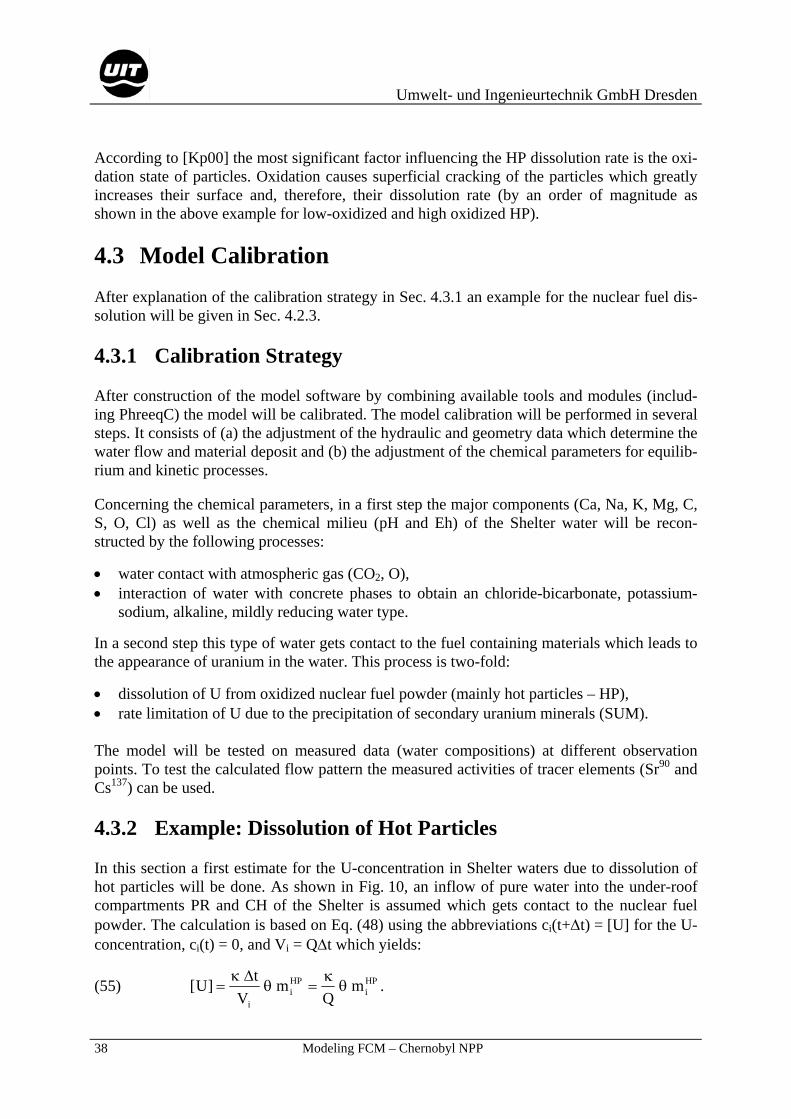
Umwelt- und Ingenieurtechnik GmbH Dresden
38 Modeling FCM – Chernobyl NPP
According to [Kp00] the most significant factor influencing the HP dissolution rate is the oxi-dation state of particles. Oxidation causes superficial cracking of the particles which greatly increases their surface and, therefore, their dissolution rate (by an order of magnitude as shown in the above example for low-oxidized and high oxidized HP). 4.3 Model Calibration After explanation of the calibration strategy in Sec. 4.3.1 an example for the nuclear fuel dis-solution will be given in Sec. 4.2.3. 4.3.1 Calibration Strategy After construction of the model software by combining available tools and modules (includ-ing PhreeqC) the model will be calibrated. The model calibration will be performed in several steps. It consists of (a) the adjustment of the hydraulic and geometry data which determine the water flow and material deposit and (b) the adjustment of the chemical parameters for equilib-rium and kinetic processes. Concerning the chemical parameters, in a first step the major components (Ca, Na, K, Mg, C, S, O, Cl) as well as the chemical milieu (pH and Eh) of the Shelter water will be recon-structed by the following processes:
• water contact with atmospheric gas (CO2, O), • interaction of water with concrete phases to obtain an chloride-bicarbonate, potassium-
sodium, alkaline, mildly reducing water type.
In a second step this type of water gets contact to the fuel containing materials which leads to the appearance of uranium in the water. This process is two-fold:
• dissolution of U from oxidized nuclear fuel powder (mainly hot particles – HP), • rate limitation of U due to the precipitation of secondary uranium minerals (SUM). The model will be tested on measured data (water compositions) at different observation points. To test the calculated flow pattern the measured activities of tracer elements (Sr90 and Cs137) can be used. 4.3.2 Example: Dissolution of Hot Particles In this section a first estimate for the U-concentration in Shelter waters due to dissolution of hot particles will be done. As shown in Fig. 10, an inflow of pure water into the under-roof compartments PR and CH of the Shelter is assumed which gets contact to the nuclear fuel powder. The calculation is based on Eq. (48) using the abbreviations ci(t+∆t) = [U] for the U-concentration, ci(t) = 0, and Vi = Q∆t which yields:
(55) HPi
HPi
i
mQ
mV
t]U[ θκ
=θ∆κ
= .

Umwelt- und Ingenieurtechnik GmbH Dresden
Modeling FCM – Chernobyl NP 39
Taking the parameters of Sec. 4.2.3, that is κ = 0.038 to 0.395 year-1 and θ = 0.1, and the HP-masses from Tab. 1 as well as the inflow rates from Tab. 2 an upper limit for the U-concentration in the Shelter water is obtained.
Fig. 10 Dissolution of HP in two upper-level compartments: PR and CH
The results are presented for low-oxidized and high-oxidized fuel particles in Tab. 11. These values overestimate the measured data for two reasons: First, during the downward flow the water gets contact only with a small fraction of the total amount of mHP in a compartment: The situation is quiet different from water flow through porous media in hydrogeology where θ represents the porosity. Adittionally, in the Shelter there is also an uncontrolled flow in channels or fractures near the walls etc. Therefore the parameter θ should account for such effects by reducing its value. This crude estimation show that θHP < 0.1. Second, in this calcu-lation no precipitation of secondary uranium minerals is taken into account. Tab. 11 Upper limits for U in water of compartments PR and CH due to dissolution of low-
oxidized and high-oxidized HP (no U-precipitation is taken into account)
compartment mass of HP [kg] water inflow rate [L/h] U-concentration [mg/L] PR 360 34.7 4 ... 47 CH 2500 162.9 7 ... 69
[Note, that from both Eq. (54) and Eq. (55) the common formula for the dissolution rate in flow experiments [Br95a, Ca94] can be derived: r = [U]Q/S, where S = mAs is the total sur-face.]
pure water
PR
Q = 34.7 L/h
mHP = 360 kg
[U]
pure water
CH
Q = 162.9 L/h
mHP = 2500 kg
[U]
Umwelt- und Ingenieurtechnik GmbH Dresden
40 Modeling FCM – Chernobyl NPP
5 Conclusion and Outlook In this report a model concept – including the mathematical framework and numerical algo-rithm – is presented for the dynamical description of chemical FCM-transformations due to the influence of water and atmosphere which results in a redistribution of contaminants inside the Shelter. It takes into account as much as possible existing data for FCM and Shelter wa-ters as well as for existing structures (premises) and established paths for water flows inside the Shelter. The importance of such model for
• understanding the contamination of Shelter waters (evolution history), • the prediction of medium and long term behavior of FCM inside the Shelter, and • the development of an optimized active leaching strategy (in case if this technology will
be applied for LFCM removal)
is evident. The measured element concentrations at the observation points (see Tab. 7) are far from being complete for a detailed chemical modeling (lack of major cations, no Eh, etc.). Thus it will be important for the model calibration to increase the number of measured element concentra-tions at the observation points (at least for the major components listed in Sec. 2.3.2).

Umwelt- und Ingenieurtechnik GmbH Dresden
Modeling FCM – Chernobyl NPP
i
References [AP93] Appelo, C.A.J., D. Postma: Geochemistry, Groundwater and Pollution, A.A. Balkema,
Rotterdam 1993.
[BN91] Ball, J.W. and Nordstrom, D.K., WATEQ4F – User’s manual with revised thermody-namic data base and test cases for calculating speciation of major, trace and redox ele-ments in natural waters, U.S.G.S. Open-File Report 90-129, 185 p, 1991.
[Bo99]
Bogatov, S.A. et al.: The Water Problem in the Object “Shelter”, report (in russian) UDK 621.039.58 (1999).
[Br95] Bruno, J., J. de Pablo, L. Daro, E. Figuerola: Experimental study and modeling of the U(VI)Fe(OH)3 surface precipitation/coprecipitation equilibria, Geochem. Cosmochem. Acta 59 (20) 4113-4129 (1995)
[Br95a] Bruno, J., I. Casas, E. Cera, J. de Pablo, J. Gimenez, M.E. Torrero: Uranium(IV) dioxide and SIMFUEL as chemical analogues of nuclear spent fuel matrix dissolution. A com-parison of dissolution results in a standard NaCl/NaHCO2 solution, Mat. Res. Soc. Proc. Vol. 353 (1995) 601.
[Ca94] Casas, I., J. Gimenez, V. Marti, M.E. Torrero, J. de Pablo: Kinetic Studies of Unirradi-ated UO2 Dissolution under Oxidizing Conditions in Batch and Flow Experiments, Ra-diochimica Acta 66/67, 23-27 (1994)
[CB98] C++Builder 3 Visual Component Library Sprachreferenz Band 1 und 2, Borland GmbH 1998.
[CB99] Borland C++Builder 4 Entwicklerhandbuch, Inprise GmbH, Langen 1999.
[Ch98] The Shelter’s Current Safety Analysis and Situation Development Forecasts (updated version), Tacis services DG IA, European Commission, November 1998.
[DA95] Diaz-Arocas, P., J. Quinones, C. Maffiotte, J. Serrano, J. Garcia, J.R. Almazan, J. Este-ban: Effect of secondary phases formation in the leaching of UO2 under simulated radio-lytic products,Mat. Res. Soc. Symp. Proc. Vol. 353 (1995) p. 641
[DS98] Domenico, A.P., F.W. Schwartz: Physical and Chemical Hydrogeology, John Wiley & Sons, Inc., New York 1998
[Dz90] Dzombak, D.A., F.M.M. Morel: Surface Complexation modeling; Hydrous Ferric Oxide, Wiley-Interscience, New York, 1990
[Fe90] Fellenberg, G.: Chemie der Umweltbelastung, B.G. Teubner Stuttgart 1990
[Gr94] Gray, W.J., S.A. Steward, J.C. Tait, D.W. Shoesmith, in High Level Radioactive Waste Managment, Proceedings of the Fifth Int. Conference, American Nuclear Society 1994, pp. 2597-2601.
[Hö96] Hölting, B.: Hydrogeologie – Einführung in die Allgemeine und Angewandte Hydro-geologie, Ferdinand Enke Verlag Stuttgart 1996
[HWS56] Handbook of Chemistry and Physics 37. edition, Hodgman, Ch.D., R.C. Weast, S.M. Selby (eds): Chemical Rubber Publishing company, CO Cleveland Ohio (1955-1956)
Umwelt- und Ingenieurtechnik GmbH Dresden
Modeling FCM – Cheronbyl NPP ii
[Ka98] Kalka, H., H. Märten, J. Hagen, R. Münze: Geochemical Infiltration Model for the Simu-lation of Reactive Transport in Mining Dump Sites, in Proceed. of the Intern. Workshop „Uranium Mining and Hydrogeology II“, Freiberg, September 1998, Verlag Sven von Loga, Köln 1998, 470 – 479.
[Kp00] Kashparov, A., V.P. Protsak, N. Ahamdach, D. Stammose, J.M. Peres, V.I. Yoschenko, S.I. Zvarich: Dissolution kinetics of particles of irradiated Chernobyl nuclear fuel: influ-ence of pH and oxidation state on the release of radionuclides in the contaminated soil of Chernobyl, Journal of Nucl. Materials 279 (2000) 225-233.
[Ku98] Kulik, D.A., V.A. Sinitsyn, I.K. Karpov: Prediction of solid-aqueous equilibria in ce-mentitious systems using Gibbs energy minimization: II. Dual thermodynamic approach to estimation of the and end-member parameters, Mat. Res. Soc. Symp. Proc. Vol. 506 (1998) 983.
[La85] Langmuir, D. and A. Riese: The thermodynamic properties of radium, Geochim. Cosmo-chim. Acta 49 (1985) 1593-1601.
[LS86]] Luckner, L. und W.M. Schestakow: Migrationsprozesse im Boden- und Grundwasser-bereich, Deutscher Verlag für Grundstoffindustrie, Leipzig 1968
[Ma90] Matthess, G.: Die Beschaffenheit des Grundwassers, Lehrbuch der Hydrologie, Band 2, Gebrüder Borntraeger, Berlin – Stuttgart, 1990.
[Me71] Merritt, R.C.: The Extractive Metallurgy of Uranium, Colorado School of Mines Re-search Institute, 1971
[MH93] Morel F.M.M., J.G. Hering: Principles and Applications of Aquatic Chemistry, John Wiley & Sons, New York 1993.
[Mo95] Morrison, S.J., R.R. Spangler, V.S. Tripathi: Adsorption of amorphous ferric oxyhydrox-ide at high concentration of dissolved carbon(IV) and sulfur(VI), J. Contamin. Hydrol-ogy 17 (1995) 333-346
[PA99] Parkhurst, David L, Appelo, C.A.J.: User’s guide to PhreeqC (version 2) – a computer program for speciation, batch-reaction, one-dimensional transport, and inverse geo-chemical calculations, Water-Resources Investigation Report 99-4259, Denver, Colorado 1999
[Par95] Parkhurst, David L.: Water-Resources Investigations Report 95-4227. Lakewood, Colo-rado 1995.
[Pau98] Paul, M., H.J. Sänger, S. Snagowski, H. Märten, M. Eckart: Prediction of the Flooding Process at the Ronneburg Site – Results of an Integrated Approach, in Proceed. of the Intern. Workshop „Uranium Mining and Hydrogeology II“, Freiberg, September 1998, Verlag Sven von Loga, Köln 1998, 130 – 139.
[SG94] Sandino, M.C.A., B. Grambow: Solubility equilibria in the U(VI)-Ca-K-Cl-H2O system – Transformation of schoepite into becquerelite and compreignacite, Mat. Res. Soc. Symp. Proc. Vol. 465 (1997) 1327.
[Si96] Sigg L., W. Stumm: Aquatische Chemie, vdf Hochschulverlag, Zürich 1996
[Sich94] Sich A.R.: The Chernobyl Accident Revisited: Source Term Analysis and Reconstruc-tion of Events during the Active Phase, Massachusetts Institute of Technology, Cam-

Umwelt- und Ingenieurtechnik GmbH Dresden
Modeling FCM – Chernobyl NPP
iii
bridge, MA 1994.
[Sin97] Sinitsyn, V.A., D.A. Kulik, M.S. Khodorivski, V.A. Kurepin, A.Y. Abramis, I.L. Koly-abina, N.A.Shurpach: Stability of mineral matter in aqueous media of the Chernobyl unit-4 shelter: thermodynamic evaluation, Mat. Res. Soc. Symp. Proc. Vol. 465 (1997) 1327.
[Sin98] Sinitsyn, V.A., D.A. Kulik, M.S. Khodorivsky, I.K. Karpov: Prediction of solid-aqueous equilibria in cementitious systems using Gibbs energy minimization: I. Multiphase aque-ous – ideal solid solution models, Mat. Res. Soc. Symp. Proc. Vol. 506 (1998) 953.
[St94] Stroustrup, B.: Die C++ Programmiersprache, Addison-Wesley, Bonn 1994
[T10] Task 10: Dust Management – Dust Report, TN/00105, Slavutych, UA, April 2000.
[T13] Task 13: Shelter Water Managment – Water Characterisation and Analysis Report, TN/00139, Slavutych, UA, April 2000.
[T14R] Selected Review of Models, report T14-R10, Chernobyl NPP, Unit 4 SIP EBP Package D “Fuel Containing Materials”, Slavutych, UA, August 1999.
[T14D] Phase 1 FCM Characterisation Plan, report T14-D1, Chernobyl NPP, Unit 4 SIP EPB, Package D “Fuel Containing Materials”, Slavutych, UA, March 2000.
[UIT00] Reclamation Concept for the Schwartzwalder Mine, Golden, Colorado; Report to Cotter Corporation Lakewood, Colorado; submitted by Umwelt- und Ingenieurtechnik GmbH, Dresden, April 2000.
[Vo90] Voigt, H.-J.: Hydrogeochemie, Springer-Verlag Berlin Heidelberg New York, 1990.