r&d: a small contribution to productivity growthd: a small contribution to productivity growth...

R&D: A Small Contribution to Productivity

Growth

DIEGO COMIN

Department of Economics, New York University

In this article I evaluate the contribution of R&D investments to productivity growth. The basis for the

analysis are the free entry condition and the fact that most R&D innovations are embodied. Free entry

yields a relationship between the resources devoted to R&D and the growth rate of technology. Since

innovators are small, this relationship is not directly affected by the size of R&D externalities, or the

presence of aggregate diminishing returns in R&D after controlling for the growth rate of output and

the interest rate. The embodiment of R&D-driven innovations bounds the size of the production exter-

nalities. The resulting contribution of R&D to productivity growth in the US is smaller than 3–5 tenths

of 1% point. This constitutes an upper bound for the case where innovators internalize the conse-

quences of their R&D investments on the cost of conducting future innovations. From a normative per-

spective, this analysis implies that, if the innovation technology takes the form assumed in the

literature, the actual US R&D intensity may be the socially optimal.

Keywords: Research and development, productivity growth, total factor productivity

JEL classification: E10, O40

1. Introduction

In this paper, I try to answer two questions: First, what has the contribution ofR&D to productivity growth been in the US during the post-war period? Afterproviding an estimate for the R&D contribution, I can answer the second: Howdoes the actual R&D intensity compare to the socially optimal intensity?The first question has been examined repeatedly before by computing the social

return to R&D in a simple econometric framework. Typically, the endogenousvariable is the Solow residual and the explanatory variables are the firm’s orindustry’s own R&D intensity and the used R&D from other firms or industries.The estimated return to own R&D ranges from 0.2 to 0.5, while for the usedR&D the estimate ranges from 0.4 to 0.8 with a total social return to R&D ofabout 70–100%.1 These numbers are very large. Indeed, since the average share ofnon-defense R&D in GDP as defined and measured by the National ScienceFoundation (NSF) over the post-war period has been 1.6%, they imply that theSolow residual is fully accounted by R&D alone.

1 See Griliches (1992), Jones and Williams (1998) and Nadiri (1993) for references.

Journal of Economic Growth, 9, 391–421, 2004

� 2004 Kluwer Academic Publishers. Manufactured in The Netherlands.

Before accepting this conclusion, we should keep in mind one important caveatto this econometric approach. Namely, that there are many factors omitted in thetypical regression that affect simultaneously TFP growth and the parties incentivesto invest in R&D. The most obvious candidates are anything that enhances dis-embodied productivity, like the managerial and organizational practices, learningby doing,. . . All these elements have a clear effect on TFP and at the same timeinduce firms to invest in R&D. Some evidence in favor of the potential impor-tance of this bias comes from the fact that, after including fixed effects in theregression, the effect of R&D on TFP growth almost disappears (Jones andWilliams, 1998).To overcome this omitted variable bias, I depart from the econometric frame-

work. Instead, I use a model with endogenous development of new technologiesto assess the importance of R&D for growth. From a methodological point ofview, I do not attempt to calibrate directly the social return to R&D in order todetermine its role on growth. My route is more indirect since it decomposes theproblem into two parts. First, I compute the effect of the amount of resourcesdevoted to R&D on the output of the R&D sector (that is the growth rate ofR&D-driven technologies). Then, I use simple growth accounting to compute theeffect of the growth of technology on productivity growth.One possible way to establish the first relationship (i.e. between the resources

devoted to R&D and the growth rate of technology) consists in calibrating theproduction function of technology. This approach, however, entails probably evenmore challenges than the traditional productivity approach because in addition tomeasuring the externalities involved in R&D, we need to specify an R&D produc-tion function. I discuss this further below in the context of a specific empiricaltest.The approach I propose in this paper, instead, exploits the free entry condition

into R&D and the fact that R&D innovations are embodied. Free entry impliesthat, in equilibrium, R&D firms break even. As a result, the cost of the resourcesdevoted to R&D equals the value of the newly developed technologies. From here,it follows that the relationship between the share of resources devoted to R&Dand the growth rate of technology is a linear function of the inverse of the marketvalue of an innovation.The advantage of using a free entry condition instead of the production func-

tion for innovations is that it is very easy to compute the private value of an inno-vation. Since innovators are small, they do not take into account the effect oftheir investment decisions on the aggregate variables when computing the value ofan innovation. Therefore, I can redo the asset pricing calculations conducted byindividual innovators where they take as given observable aggregate variables tocalculate the private value of an innovation. Then, I can use the free entry condi-tion to calibrate the growth rate of new technologies for a given R&D intensitywithout having to take any stand on the specification or calibration of the produc-tion function for new technologies.To implement this exercise, I follow most of the productivity literature by using

the NSF data on R&D. The NSF measures the resources spent towards the

DIEGO COMIN392

development of new knowledge, products and processes by workers with trainingin physical sciences. It is important to understand that these innovations affect theproduction of final output mostly through the development of new goods.2 In thatsense, the innovations that result from the R&D activities, as measured by theNSF, represent by and large innovations that are embodied in the sense of Solow(1959). This means that a firm can only benefit from R&D by using the goods thatresult from the R&D activities.3’4

The results I obtain are quite striking given the existing consensus about theimportance of R&D for growth.5 The average annual growth rate of productivityin the US during the post-war period has been 2.2% points. Less than 3–5 tenthsof 1% point are due to R&D.The intuition for this small contribution is quite simple. The few resources

devoted to R&D signal a small private value of the innovations. But, as the bulkof the productivity literature has argued, there may be significant externalities thatlead to large productivity gains even with few R&D investments. These externali-ties can appear in the production of final output or in the R&D process.Production externalities arise because the development of one innovation has an

effect on labor productivity beyond its contribution to the capital stock (i.e. itaffects the Solow residual). When innovations are embodied, firms enjoy produc-tion externalities to the extent that they use the new goods. Further, a larger pro-duction externality implies that, for a given number of available innovations, thedemand faced by new innovators is higher. Therefore, ceteris paribus, the marketvalue of an innovation is positively correlated with its social value. In terms of mytwo-step approach, this means that a larger production externality raises the effectof the growth of technology on productivity growth but reduces the growth oftechnology associated with a given R&D intensity. As a result, the R&D contribu-tion to productivity growth is not very sensitive to the size of the externalities inproduction.R&D externalities associate past R&D investments with a reduction in the

cost of developing future innovations. To show the inconsistency of large R&D

2 Process innovations can be thought as resulting in the development of new goods that replace the

old ones. The model used in the next section to calibrate the R&D contribution to productivity

growth naturally accomodates this mechanism.

3 Of course, R&D labs could benefit from the knowledge created in previous R&D efforts. These

R&D externalities are addressed below. I will not consider, however, the possibility that final

output firms benefit from the knowledge created in the labs without using the goods that embody it.

4 Clearly, there are other (non-R&D) intentional investments that lead to improvements in

productivity. These investments are mostly disembodied in the sense that, to enjoy the gains in

productivity, firms do not need to adopt any new capital or intermediate good. A few examples

in this category are: the resources Henry Ford devoted to improve the mass production system,

McKinsey’s reports, the resources devoted to develop better personnel and accounting practices,

or any other managerial innovation.

5 The only exception to this consensus is the BLS who reports a R&D contribution to total factor

productivity growth of 0.2% points. This difference steams from the rate of return for R&D that

the BLS imputes which is substantially lower than in the rest of the literature.

R&D: A SMALL CONTRIBUTION TO PRODUCTIVITY GROWTH 393

externalities and a low R&D intensity in steady state, suppose for a moment thatthe R&D externalities were large and that the economy is in steady state. Then, asmall R&D intensity today, can generate a large growth rate of technology that inturn generates a large reduction in the costs of developing innovations tomorrow.As a result, tomorrow, agents want to devote a large share of resources intoR&D; but this is inconsistent with the fact that the share of resources devoted toR&D is constant in steady state. Therefore, the observed low R&D intensity indi-cates that R&D externalities cannot be very large.The free entry condition establishes a relationship between the R&D intensity

and the growth rate of technology that can be used to calibrate the size of theR&D externalities. Once this is done, we can solve the social planner’s problem.This entails determining how much she would invest in R&D with the calibratedproduction structure. Then we can compare this socially optimal R&D intensitywith the actual intensity in order to answer the second question posed in thispaper. Specifically, I find that the observed R&D intensity may be quite close tothe socially optimal intensity.The rest of the paper is structured as follows. Section 2 contains the baseline cali-

bration One clear goal of this paper is to show that the magnitude of the calibratedR&D contribution to productivity growth is very robust. Section 3 tries to show thisby considering more general production functions that accommodate more flexiblerelationships between R&D-driven technology and productivity growth. This analy-sis emphasizes the importance that R&D innovations are embodied. In this sense,this paper contributes to the literature started with Phelps (1962) on the relevance ofthe decomposition between embodied and disembodied technological progress. InSection 3.1, I investigate some elements that affect the relationship between the shareof resources devoted to R&D and the growth rate of technology (for example thepresence of increasing returns in the production of R&D-driven technologies, inter-national spillovers,...). Section 3.2 discusses the robustness of the results to consider-ing production functions that allow for more general relationships between thegrowth rate of new technologies and productivity growth. In Section 3.3, I move outof the steady state and consider how the calibrations would change had the US econ-omy been in transition to the steady state. In Section 4, I discuss the limits of theapproach proposed in this paper. Section 5 draws the welfare implications of the pre-vious analysis. Section 6 concludes.

2. The Basic Argument

Throughout the paper I use _X to designate the time derivative of a generic vari-able X , and cX to denote the growth rate of variable X : Let us denote by A thelevel of technology associated with R&D investments. In the terminology of Ro-mer (1990) or Grossman and Helpman (1991, chapter 3), this is the number ofvarieties though I will show later that this framework can accommodate otherinterpretations. To compute the R&D contribution to productivity growth, I startby investigating the relationship between the amount of resources devoted to

DIEGO COMIN394

R&D (expressed in units of final output, which is the numeraire), R, and thegrowth rate of technology. Then I use a production function to relate the growthrate of A to the growth rate of labor productivity.Let PA denote the market price of a firm that has earned a patent to produce

one of these varieties. The free entry condition implies that innovators make zeroprofits in equilibrium, therefore the cost incurred to develop the patent (R) is equalto the market value of the flow of new technologies (PA

_A).6

PA_A ¼ R: ðFree EntryÞ

The free entry condition yields the following expression for the growth rate ofR&D-driven technologies

cA ¼ sY

PAA; ð1Þ

where Y denotes the economy-wide output, s denotes the share of resourcesdevoted to R&D (i.e. s � R

Y). To establish the link between R&D intensity (s) andthe growth rate of R&D-driven technologies (cA) we just need to find an expres-sion for Y

PAA: For that it is necessary to specify a production function and to price

the stock of patents.Final output (Yt) is produced out of labor (Lt) and intermediate goods (xit). In

particular, I assume the functional form in equation (2)

Yt ¼ ZtL1�at

XAt

i¼1

xaqit

!1q

; ð2Þ

where Zt denotes the level of non-R&D-driven technology.7

Standard profit maximization implies the following inverse demand curve forintermediate goods

pit ¼ aL1�at

XAt

i¼1

xaqit

!1q�1

xaq�1it ;

where pit denotes the price of the ith variety.To produce one unit of intermediate goods producers need to use a unit of capi-

tal whose rental price is r.8 Innovators can charge a markup (g) above the mar-ginal cost of production either because they earn a patent or because they keepsecret the blueprint of the innovation. Optimal pricing of the intermediate goods

6 For the argument to go through, we just need this relationship to hold in the long-run because our

interest is on the determinants of long-run productivity growth.

7 This specification introduces a wedge between the capital share (a) and the elasticity of substitution

across different varieties which is equal to aq.8 The calibrated effect of R&D on growth is independent of the rate of transformation between final

output and intermediate goods. This parameter that here is normalized to 1 just cancels out.


that embody the innovations implies that the markup is constant and equal to theinverse of the elasticity of substitution between the different intermediate goods(i.e. g ¼ ðaqÞ�1Þ.After some algebra, it follows that the static operating profits earned by an

innovator can be written as

p ¼ g� 1

gaY

A: ð3Þ

From here, it follows that

Y

A¼ pg

aðg� 1Þ : ð4Þ

To close the first step in the argument, we just have to derive the market price ofan innovation. Suppose for simplicity that patents do not expire and that innova-tors are not overtaken by new innovators with more sophisticated capital goods.Then the value of an innovation, PA; must satisfy the following asset equation:

rPA ¼ pþ _PA; ð5Þwhere r is the relevant discount rate.From equation (5) it follows that

PA ¼ pr � cPA

: ð6Þ

In steady state, all variables grow at constant rates. From equation (1), thisimplies that

cPA¼ cY � cA: ð7Þ

Substituting expressions (4), (6) and (7) into equation (1) and isolating cA weobtain the following expression for the growth rate of technology in terms of s:

cA ¼ r � cYg�1g

as � 1

: ð8Þ

There are two important observations from this expression. First, the link betweencA and s does not come from a production function for technology; it follows fromthe positive relationship that the free entry condition (1) defines between the two.Second, cA in expression (8) does not depend directly on the size of the externalitiesin R&D or on the degree of the diminishing returns to aggregate R&D invest-ments;9 note that I have not even specified the production function for the creationof technologies. This is the case because we have mimicked the calculations madeby small innovators that want to figure out the market price of their innovations

9 In Section 3.1.4 and in Comin (2002) I generalize the analysis to allow for dynamic increasing

returns in R&D at the firm level by conceding incumbents a cost advantage in subsequent R&D.

DIEGO COMIN396

(PA) and do not take into account the effect of their investment decisions onaggregate variables like the interest rate or the growth rate of output. Since theexternalities appear through these aggregate variables, we do not need to calibratethem once we control for cY and r.The second step in the computation of the R&D contribution to productivity

growth consists of using the production function (2) to relate the growth rate ofR&D-driven technology (cA) to the growth rate of productivity. From there it fol-lows that

cY=L � cY � cL ¼ cZ þ1

qcA þ aðcx � cLÞ: ð9Þ

To solve for cx, I take advantage of the symmetry of the intermediate goods inproduction. From the pricing rule and the inverse demand function, it followsthen that

xi ¼ L aZA

1�qq

gr

! 11�a

:

In steady state r is constant and therefore cx � cL ¼ 1�qqð1�aÞ cA. Plugging this back

into (9), we obtain the following expression for the growth rate of productivity:

cY=L ¼ 1

1� acZ þ

1

q1� aq1� a

� �cA

zfflfflfflfflfflfflfflfflfflffl}|fflfflfflfflfflfflfflfflfflffl{:

Contribution of R&D to productivity growth

ð10Þ

Using the expression for the optimal markup and (8) we can rewrite the contribu-tion of R&D to productivity growth as follows:

Contribution of R&D to productivity growth ¼ a1� a

r � cY

g�1 as � ðg� 1Þ�1

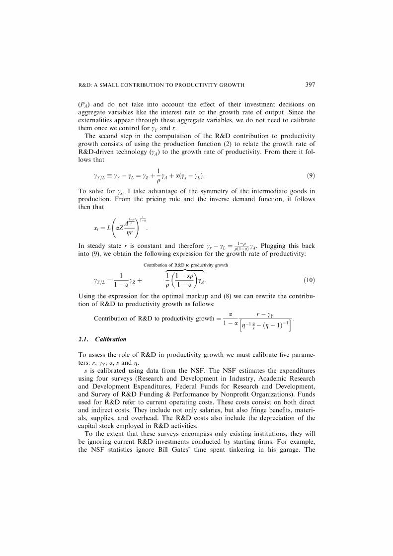
h i :2.1. Calibration

To assess the role of R&D in productivity growth we must calibrate five parame-ters: r; cY ; a; s and g:s is calibrated using data from the NSF. The NSF estimates the expenditures

using four surveys (Research and Development in Industry, Academic Researchand Development Expenditures, Federal Funds for Research and Development,and Survey of R&D Funding & Performance by Nonprofit Organizations). Fundsused for R&D refer to current operating costs. These costs consist on both directand indirect costs. They include not only salaries, but also fringe benefits, materi-als, supplies, and overhead. The R&D costs also include the depreciation of thecapital stock employed in R&D activities.To the extent that these surveys encompass only existing institutions, they will

be ignoring current R&D investments conducted by starting firms. For example,the NSF statistics ignore Bill Gates’ time spent tinkering in his garage. The


omission of these expenditures is probably not very relevant from a quantitativepoint of view. This claim follows from the fact that in 1999 only 4% of totalindustrial R&D came from firms with less than 25 employees. This number is anupper bound for the average share of R&D from small firms for the post-war per-iod since in 1998 it was only 3% and in 1997, the share of industrial R&D fromsmall firms was only 2%. Since most start ups become small incorporated firmsand continue doing R&D (surely more intensively than before incorporation),these small fractions should give us an idea of the small magnitude of the bias.Figure 1 plots the evolution of the share of US non-defense R&D expenditures

in the US GDP as reported by the NSF. The average over the post-war period isabout 1.6%. In my calibrations, I use a value for s of 0:02; which is an upperbound for the average share of resources devoted to non-defense R&D during thepost-war period in the US.r is calibrated to the average real stock return in the US post-war period from

Mehra and Prescott (1985). Pakes and Schankerman (1984) provide evidence thatthis is approximately the private rate of return to R&D once we take into accountthe obsolescence of patents and the gestation lags that I incorporate in the nextsection. The average real growth rate of output (cY ) between 1950 and 1999 in theUS reported by the BLS is 0.034. a is calibrated to 1/3 to match the capital sharein the post-war period: For the markup (g) I explore two values: 1.2 and 1.5. Thelatter is on the upper limit of the intervals given by Basu (1996) and Norrbin(1993) for the average markup in the economy. However, I regard this as more

0

0.5

1

1.5

2

2.5

1953

1955

1957

1959

1961

1963

1965

1967

1969

1971

1973

1975

1977

1979

1981

1983

1985

1987

1989

1991

1993

Figure 1. US share of non-defense R&D expenditures in GDP in percentage points. Source: NSF.

DIEGO COMIN398

realistic since the markups charged by innovators should be well above the aver-age markup in the economy because of the monopolistic power conferred by thepatent system and because the higher ratio of the up front fixed cost to the mar-ginal cost of production for technological goods than for non-technological goodsor services (Table 1).10

Figure 2 displays the R&D contribution to productivity growth for various lev-els of R&D intensity and for the two values of the markup. The first thing thatstands out from this figure is that for R&D intensities similar to the observed inthe US post-war period (i.e. around 2%), the R&D contribution to productivityrepresents only about a tenth of the average annual growth rate of productivity inthe post-war period (2.2%). For the higher markup (g ¼ 1:5Þ even an R&D inten-sity three times larger than the observed in the US (6%) only would account forhalf of the growth rate of productivity observed in the post-war period. For the

0.000

0.005

0.010

0.015

0.020

0.025

0.030

0.015 0.020 0.024 0.029 0.033 0.038 0.042 0.047 0.051 0.056s

eta=1.2 eta=1.5

Figure 2. R&D contribution to productivity growth in the baseline model.

Table 1. Parameters.

r 0.07

cY 0.034

a 0.33

s 0.02

g {1.2, 1.5}

10 Results hold a fortiori if g is calibrated to a higher value.


low (less realistic) markup (g ¼ 1:2Þ; an R&D intensity of 4% is necessary toaccount for half of the post-war productivity growth rate. To account for all thepost-war productivity growth the required R&D intensities are 4.8% for the lowmarkup case and 8% for the high markup.Of course, there are other factors not considered here such as investments in

human capital that may contribute to productivity growth. In this sense, onemay want to compare the predicted R&D contribution to growth with the aver-age TFP growth rate in the US during the post-war period that has been 1.4%.This alternative metric, however, does not change the flair of the conclusionsfrom the analysis.In other calibrations not reported here, I have observed that the small R&D

contribution to productivity growth is very robust to the parameterization of theinterest rate (r). This allows me to extend the results to environments where theopportunity cost of R&D investments is higher because innovators are credit con-strained or more risk averse.The small contribution of R&D is the result of three effects. First, the low R&D

intensity observed in steady state implies that the externalities in the R&D processare small. Otherwise, future R&D investments would be very profitable and weshould observe a large R&D intensity. Second, the small R&D intensity also impliesthat the growth rate of A for any given markup (within reasonable bounds) must berelatively low. Finally, in this environment where R&D innovations affect produc-tivity through the goods that embody them, the contribution of production exter-nalities to productivity growth is equal to ð1q � aÞcA: For given a and cA; a lowerelasticity of substitution across the different intermediate goods increases the size ofthe production externalities. However, a reduction in the elasticity of substitutionalso raises the markup (g). Naturally, this results in a higher PA and, from the freeentry condition, in a lower cA for any given R&D intensity sð Þ. In other words, as Iwill emphasize in Section 3.2, the embodiment assumption introduces a trade offbetween the growth rate of R&D-driven technology and the size of the productionexternalities that bounds the R&D contribution to productivity.

3. Extensions

Now, I extend the baseline model along several dimensions to show that the sizeof the R&D contribution to productivity growth is robust. The first group ofextensions deals with considerations that affect the private value of an innovation.These include the obsolescence of innovations, the presence of international spill-overs in R&D investments, R&D lags, the imitation of innovations, and the possi-bility of successive R&D for incumbent firms (i.e. firm-level increasing returns toR&D). The second extension generalizes the production function to capture moregeneral externalities in the production of final output. Finally, I relax the assump-tion that the economy is in steady state and compute the R&D contribution toproductivity growth if the US economy had been in transition during the post-warperiod.

DIEGO COMIN400

3.1. The Value of Innovations

In the free entry condition, equation (1), we can see that the relationship betweenthe share of resources devoted to R&D and the growth rate of technology is medi-ated by the value of innovations. Therefore, in principle, the R&D contribution togrowth could be increased by enriching the model with new dimensions of theR&D process that affect the value of innovations. Next, I show that the smallcontribution is robust to many variations.

3.1.1. Creative Destruction

To incorporate the firm dynamics that characterize the Schumpeterian models ofAghion and Howitt (1992) and Grossman and Helpman (1991, chapter 4) I followJones and Williams (2000). They introduce the concept of innovation clusters tocapture the idea that innovations come in bunches and that firms must adopt allof the innovations in a cluster to actually benefit from it. Say, out of everyðwN þ wÞ intermediate goods developed, only wN are completely new. The rest arejust new versions of existing intermediate goods that are necessary to use the newintermediate good. These new versions are otherwise identical to the existingones.11 When a new cluster is adopted, the new versions of existing intermediategoods replace the old versions and this limits the expected life-time of an innova-tion.When a new technological cluster is developed, the incumbents may try to pre-

vent the diffusion of the new technological cluster by reducing their prices. Thisintroduces some richer interactions in the pricing of intermediate goods. In partic-ular, two scenarios are possible. It may be the case that these reactions do notconstrain the pricing decisions of the innovators. Then the innovator charges themonopolist price, p ¼ r= aqð Þ: Alternatively, the limit pricing rule may be binding.Since in reality we observe that new products are developed and adopted I focuson the equilibrium where new intermediate goods are immediately adopted.12

After imposing this restriction we can derive the limit pricing rule that is consis-tent with the adoption of new varieties. Jones and Williams [2000], show that themarkup under limit pricing is

gL ¼ wN

wþ 1

� � 1aq�1

:

11 A simple example that illustrates this concept is a CD writer. Before the CD writer was developed,

we just had a CD reader and a software for this to work. Now with the CD writer, we must

modify the CD reader’s software to make possible the interaction between the two drives. In this

case, w ¼ 1 (the software) and wN ¼ 1 (the CD writer).

12 If this is not the case, there is no reason to undertake R&D investments.


Intuitively, the higher the ratio of the number of new goods to the number ofcomplementary goods that must be changed to use the new innovation (

wN

w ), thelower is the limit markup because more incumbents are willing to reduce theirprices to prevent adoption. Quite naturally, the limit price is also decreasing in theelasticity of substitution across intermediate goods. The resulting price for inter-mediate goods is pit ¼ grt where

g ¼ min1

aq

z}|{monopolistic markup

; 1þ wN

w

� � 1aq�1

zfflfflfflfflfflfflfflfflfflffl}|fflfflfflfflfflfflfflfflfflffl{limit pricing markup8>>>><>>>>:

9>>>>=>>>>;:

The new free entry condition is now

PAwN þ wwN

_A ¼ R: ð11Þ

The price of innovations must also satisfy the following asset equation:

rPA

z}|{opportunity cost

¼ pz}|{profit flow

þ _PA �wwN

cAPA

zfflfflfflfflfflfflfflfflfflffl}|fflfflfflfflfflfflfflfflfflffl{capital gain

:

From here it follows that

cA ¼ r � cYg�1gð Þas � 1

� �1þ w

wN

� � ; ð12Þ

and that the R&D contribution of to productivity growth is

R& D contribution to productivity ¼ 1

q1� aq1� a

� �cA:

I do not attempt to calibrate wwN.13 As in the baseline model, q is calibrated by

exploiting its relationship with the markup. Now there are two cases dependingon whether the innovator can charge the monopolistic markup or whether she isforced to use the limit pricing rule.Case 1: If g ¼ 1

aq then 1q ¼ ga: Figure 3 plots the contribution of R&D to pro-

ductivity growth for different values of g and wwN

for an R&D intensity of 2%. Inthe figure we can see that under monopolistic pricing the contribution of R&D togrowth is bounded above by 2 tenths of 1% point. That is, R&D cannot account

13 This could be done by using data on the average life span of a patent or, when more sophisticated

concepts of firms are introduced, on the average life span of a firm or on the average number of

patents held by an innovator.

DIEGO COMIN402

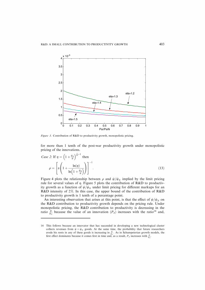
for more than 1 tenth of the post-war productivity growth under monopolisticpricing of the innovations.

Case 2: If g ¼ 1þ wN

w

� � 1qa�1

then

q ¼ a 1þ lnðgÞln 1þ wN

w

� �0@

1A

24

35�1

: ð13Þ

Figure 4 plots the relationship between q and w=wN implied by the limit pricingrule for several values of g. Figure 5 plots the contribution of R&D to productiv-ity growth as a function of w=wN under limit pricing for different markups for anR&D intensity of 2%. In this case, the upper bound of the contribution of R&Dto productivity growth is 1 tenth of a percentage point.An interesting observation that arises at this point, is that the effect of w=wN on

the R&D contribution to productivity growth depends on the pricing rule. Undermonopolistic pricing, the R&D contribution to productivity is decreasing in theratio w

wNbecause the value of an innovation PAð Þ increases with the ratio14 and,

0 0.1 0.2 0.3 0.4 0.5 0.6 0.7 0.8 0.9 10

0.5

1

1.5

2

2.5

3

3.5

4x 10-3

Psi/PsiN

eta=1.2 eta=1.3

eta=1.4

eta=1.5

Figure 3. Contribution of R&D to productivity growth, monopolistic pricing.

14 This follows because an innovator that has succeeded in developing a new technological cluster

collects revenues from wþ wN goods. At the same time, the probability that future researchers

erode his rents in any of these goods is increasing in wwN

: As in Schumpeterian growth models, the

first effect dominates because it comes first in time and, as a result, PA increases with wwN.


0 0.1 0.2 0.3 0.4 0.5 0.6 0.7 0.8 0.9 11.8

2

2.2

2.4

2.6

2.8

3

Psi/PsiN

eta=1.2

eta=1.3

eta=1.4

eta=1.5

Figure 4. qðw=wN jgÞ.

0 1 2 3 4 5 6 7 8 9 100

0.2

0.4

0.6

0.8

1

1.2

1.4

1.6

1.8

2x 10-3

Psi/PsiN

eta=1.2

eta=1.3

eta=1.4

eta=1.5

Figure 5. R&D Contribution to productivity growth under limit pricing.

DIEGO COMIN404

from free entry, this reduces the growth rate of A consistent with the observedR&D intensity: When innovations’ prices are limited by the prices of the previousinnovations, the contribution is increasing in w=wN because, in addition to the pre-vious effect, now q decreases in w=wN ; for any given markup, as illustrated in Fig-ure 4: As we have just argued, the size of the production externalities decreaseswith the elasticity of substitution across varieties, and therefore it increases in theratio w=wN . This effect dominates the effect on PA and, as a result, the R&D con-tribution to productivity increases with w=wN .

3.1.2. Correlated Shocks

In the baseline model we have assumed that the obsolescence shocks are inde-pendent across the different intermediate goods in a common innovation clus-ter. This is probably not a very realistic assumption. When a new technologicalcluster is developed, there is a chance that it drives out of the market a largenumber of intermediate goods of an older cluster. In this scenario, the shocksfaced by the intermediate goods in a given cluster are highly correlated. In Co-min (2002) I model this idea in the simple case where each new technologicalcluster makes completely obsolete an older cluster. This is precisely the struc-ture of the simple quality ladder models. It turns out from my analysis thateven after introducing correlated shocks and R&D lags, the contribution ofR&D to productivity growth for the more reasonable markups is boundedabove by 3–5 tenths of 1% point.

3.1.3. Imitation

Another relevant extension consists of relaxing the assumption of perfectenforcement of patents. If imitators are able to copy the goods developed bythe innovators, the value of innovations declines and the free entry conditionyields a higher growth rate of A for any given R&D intensity. Nevertheless,imitation does not affect substantially the R&D contributions to productivitygrowth computed above. Mansfield el al. (1981) have information about theprobability that an innovation is imitated and about the average cost of imita-tion. If in addition we recognize that imitations are not more valuable than theoriginal innovations, then we can easily redo our calculations and observe thatthe R&D contribution to productivity growth is bounded above by 3–5 tenthsof 1% points.15

15 Probably, this upper bound overstates the contribution of R&D because some of the imitation

expenses are likely to be reported as research and development expenses in the NSF surveys. This

would have the effect of reducing s in our calculations, and from the free entry condition, would

result in a lower cA and in a lower contribution to productivity growth.


3.1.4. Subsequent R&D Cost Advantage

Up to now, a firm has been characterized by the set of varieties that form an inno-vation cluster. All of these intermediate goods are developed simultaneously andonce they become obsolete the firm vanishes. However, the evidence tells us that alarge fraction of innovations are developed by firms that have already developedsome other innovation clusters. This can be due to the fact that the costs of inno-vation decline with the number of varieties developed (i.e. there is some form ofincreasing returns to R&D at the firm level). If this is the case, innovations aremore valuable than what we have computed so far. Investing in R&D not onlygrants the right to future revenues from the new innovation cluster but also theoption to develop more clusters in the future at a lower cost. To reconcile thehigher value of innovations with the observed low s, the free entry condition nowdictates a lower growth rate of varieties and a smaller contribution of R&D toproductivity growth.This additional complexity is useful to generalize the argument made above to

large firms. These internalize part of the positive consequences of their invest-ment decisions. By taking advantage of part of the externalities, the value of theR&D firm increases, and the growth rate of varieties induced by a given shareof R&D is lower than when firms are small. Hence, the benchmark contributioncomputed above gives an upper bound for the role of R&D in productivitygrowth when firms are allowed to grow. Comin (2002) shows this statements for-mally.

3.1.5. R&D Lags

In reality there is a lag between the outlay of the R&D investment and the begin-ning of the associated revenue stream. This lag corresponds both to the lagbetween project inception and conception (the gestation lag), and the time fromproject completion to commercial application (the application lag). Rapoport(1971) and Wagner (1968) have gathered data on lags for 52 technologies in vari-ous manufacturing sectors and have found that these lags range between 1.5 and2.5 years. In Comin (2002) I show that introducing these lags in the analysis has avery small effect on the previous calculations.

3.1.6. International Technology Flows

Intermediate goods flow internationally. The new technologies developed in Japancan be purchased in the US and used in the production of final output. Thisobservation has two implications for the baseline analysis. On the one hand, Ishould use the R&D investments conducted in the whole world, and not just inthe US, to calibrate the R&D intensity. On the other, a US innovator now can sellher innovation to the whole world, and therefore I should take into consideration

DIEGO COMIN406

the effect of this larger market size on the value of innovations. In terms of ourcalibration, the first effect implies that now the free entry condition is

PAw

ðwþ wN ÞwN

_A ¼ Rw; ð14Þ

where Rw represents the R&D in the world. Following the same logic as above,PAw can be expressed as:

PAw ¼ wNswðwþ wN ÞcA

YwA

; ð15Þ

where Yw and sw denote respectively the world level of output and the share ofR&D in the world’s output.The second effect implies that the profits of a successful innovator are a func-

tion of the output of the countries where she can sell her innovations. Since inno-vations can be sold internationally, the new profit flow from a new variety is:

pw ¼ g� 1

g

� �aYwA

:

As before, the value of an innovation is determined in the market and must satisfyan asset equation.

r ¼ pwPAw

þ cPAw� wwN

cA: ð16Þ

The last term on the right-hand side is the same as in the closed economy case. Insteady state, equation (15) implies that cPAw

is equal to cYw�cA: But the interestingaction takes place in the profit rate. There we can see that the two consequencesfrom the internationalization of the economy exactly cancel out. More specifically,

pwPAw

¼g�1g

� �a wN þ wð Þsw wN

cA:

Intuitively, the international flow of intermediate goods raises the resourcesdevoted to develop the varieties that are ultimately used in the production of USoutput. The flip side of the coin is that US’ (and any other country’s) innovatorscan sell their goods to a larger market. Since both forces are proportional to Yw,they cancel out.16

Plugging this expression into the asset equation (16), we obtain the followinggrowth rate of innovations:

16 This is not the case if international partners engage in R&D but the US innovators cannot export

their products. This scenario, however, seems empirically irrelevant.


cA ¼ r � cYwg�1gð Þasw

� 1

� �1þ w

wN

� � ð17Þ

It is easy to see that the figures obtained cannot be larger than the ones obtainedin the previous section. Note from expression (17) that cA is increasing in sw anddecreasing in cYw . In the post-war period, the growth rate of output in the OECDhas been higher than in the US, and the share of R&D in GDP is higher in theUS than in the OECD. Therefore, the upper bounds for the R&D contribution toproductivity growth are unaffected by introducing international considerations.Since we have not specified a production function for new technologies, this con-clusion holds for production functions that capture all sorts of international spill-overs in R&D.

3.2. More General Production Functions17

In the baseline model, the elasticity of productivity growth with respect to cA isequal to 1�aq

q þ a 1�aqð Þq 1�að Þ , where the first term corresponds to the static externality of

A on output and the second to the capital deepening driven by the development ofnew technologies. One might argue that with a more general production functionwe could parameterize the externality in production in such a way that R&D gen-erates an arbitrarily large growth rate of productivity. One such production func-tion would be

Y ¼ ArZ

Z A

0xaqi

� �1q

:

In this production function, by increasing r we can increase the size of the pro-duction externality and the R&D contribution to growth. However, note also thatin this production function R&D innovations are not embodied. Firms do notneed to buy a single unit of the latest innovation to benefit from the productivitygains associated with this innovation. But this is not consistent with the NSF defi-nition of R&D.In what follows, I show that if R&D technologies are embodied the R&D contri-

bution to productivity does not depend very much on the size of the productionexternalities. Intuitively, the variable production externality introduces a wedgebetween the effective level of R&D-driven technology and A: The embodied nature

17 In this analysis I have assumed that the production function of final output is Cobb–Douglas.

Basu (1996), Burnside, et al. (1995) and Berndt (1976) among others have shown that a Cobb–

Douglas is a good approximation to the US data. Further, in the working paper version of this

article (Comin, 2002) I show that the growth rate of R&D innovations is not very sensitive to the

elasticity of substitution between capital and labor.

DIEGO COMIN408

of R&D innovations implies that to benefit from them, firms must purchase thegoods that embody these innovations. If the elasticity of the effective level of R&Dtechnology with respect to A is larger than one, the efficiency of an innovationgrows with its vintage. Moreover, a larger production externality generates a highereffective level of technology embodied in a new good, for a given A, and this, inturn, induces a larger demand and a higher value for the innovations. Hence, whenR&D innovations are embodied, the free entry condition implies that a higher pro-duction externality reduces the growth rate of A associated with a given R&Dintensity. This effect introduces a trade off that limits how much productivitygrowth can be explained by increasing the size of the production externalities.To see this more formally, consider an environment that is exactly the same as

in the baseline model but with the following aggregate production function:

Y ¼ ZL1�aZ A

0aix

aqi di

� �1q

;

where now the level of R&D-driven technology is a continuous variable and thecapital varieties have different efficiencies ai. To introduce some flexibility on thesize of the production externality, I set ai ¼ bir�1; where b is any positive constantthat, without loss of generality, I normalize to 1, r > aq and i is a technologyindex. The size of the externality in production is increasing in r. When r > 1;newer innovations are more efficient than older innovations.The inverse demand for a particular variety i; is

pi ¼ ZaL1�aZ A

0aix

aqi di

� �1q�1

aixaq�1i :

Due to the isoelastic nature of the demand, innovators set a price equal to a con-stant markup g times the marginal cost of production r: Following the same alge-braic steps as in the standard model, we can easily find that when the state of theart technology has index A; the level of output is given by expression (18) and theprofits for an innovator that developed a variety with index i � A are given by(19).18

Y ¼ LZ1

1�aaa

1�a grð Þ�a1�aA

r�aqq 1�að Þ; ð18Þ

18 It can also be shown that

K ¼Z A

0aixi di ¼ vKZ

11�aLA

r�aqð Þ 1�qð Þþq 1�að Þ 2r�1�raqð Þq 1�að Þ 1�aqð Þ ;

where vK is a positive constant; and that

Y ¼ vY ZA~rKaL1�a;

where vY is another positive constant and ~r ¼ r 1�aqð Þq .


piA ¼ g� 1

gar� aq1� aq|fflfflffl{zfflfflffl}Level effect

Y

A

i

A

� � r�11�aq

|fflfflfflffl{zfflfflfflffl}Gradual substitution

: ð19Þ

In this last expression, we can distinguish two effects of r on the profits of aninnovator. The higher curvature in the efficiency of capital vintages (r), the higherthe initial level of profits, but also the faster final good producers gradually substi-tute towards the new, more efficient, varieties.Expression (19) can be rewritten in terms of the vintage of the variety sold by

the innovator. More specifically, let vi be the vintage of the ith variety. In steadystate, A grows at the constant rate cA. Let us suppose that the economy started onthe balanced growth path. Then the profits at time t of an innovator that devel-oped a vintage vi variety are:

pvit ¼g� 1

gaY

A

r� aq1� aq

e�r�11�aqð Þ t�við ÞcA : ð20Þ

When r > 1, the innovations embodied in newer varieties are more profitable thanthose embodied in older vintages. The converse is true when r < 1: Consequently,the market value of an innovation generically varies in the cross-section. Let PAt;v

denote the price at time t of a vintage v innovation. From free entry, we know that

PAtt ¼swN

cA wN þ wð ÞY

A: ð21Þ

Since PAtv is determined in the market, it satisfies the following differential equation:

rPAtv ¼ pvt þ _PAtv �wwN

cA: ð22Þ

It is easy to see that PAtv ¼ PAtt e�cA

r�11�aqð Þðt�vÞ.19 This implies that

cPAtv¼ cY � cA

r�aq1�aq

� �. Dividing both sides of equation (22) by PAvt and plugging

(20 ) and this expression for cPAtv; we can derive expression (23).

cA ¼ r � cYg�1gð Þas 1þ w

wN

� �� 1

� �r�aq1�aq

� �� w

wN

: ð23Þ

This expression differs from the growth rate of technology in the baseline model(12) in two respects. First, the profit rate of innovations increases with r . Second,a higher r implies a higher expected capital loss due to the depreciation of the mar-ket value of the innovations. The first effect raises the current value of an innova-tion while the second reduces it. However, in expression (23) it is clear that the first

19 For this one can solve the differential equation (22) plugging in (20) and using the initial condition

(21).

DIEGO COMIN410

force dominates the second, and the higher is the externality in production (r0) thelower is the growth rate of technology associated with a given R&D intensity.To complete the calculation we just need to derive the growth rate of productiv-

ity from expression (18).

cY=L ¼ 1

1� acZ þ

r� aqqð1� aÞ cA:

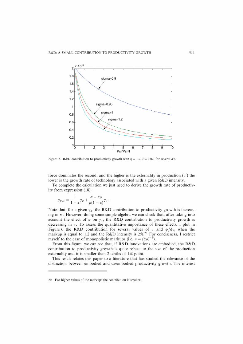
Note that, for a given cA; the R&D contribution to productivity growth is increas-ing in r . However, doing some simple algebra we can check that, after taking intoaccount the effect of r on cA; the R&D contribution to productivity growth isdecreasing in r. To assess the quantitative importance of these effects, I plot inFigure 6 the R&D contribution for several values of r and w=wN when themarkup is equal to 1.2 and the R&D intensity is 2%.20 For conciseness, I restrictmyself to the case of monopolistic markups (i.e. g ¼ ðaqÞ�1).From this figure, we can see that, if R&D innovations are embodied, the R&D

contribution to productivity growth is quite robust to the size of the productionexternality and it is smaller than 2 tenths of 1% point.This result relates this paper to a literature that has studied the relevance of the

distinction between embodied and disembodied productivity growth. The interest

0 1 2 3 4 5 6 7 8 9 100

0.2

0.4

0.6

0.8

1

1.2

1.4

1.6

1.8

2x 10-3

Psi/PsiN

sigma=0.9

sigma=0.95

sigma=1

sigma=1.2

Figure 6. R&D contribution to productivity growth with g ¼ 1:2; s ¼ 0:02; for several r’s.

20 For higher values of the markups the contribution is smaller.


in this question started with Phelps (1962) who showed that the elasticity of thesteady state level of output with respect to the savings rate does not depend onthe composition of technological progress.21 On the empirical front, Denison(1964) argued that embodied technological change represents a small fraction ofproductivity growth. Twenty years later, McHugh and Lane (1987) came out withbetter estimates that controlled for the cyclical variation in the utilization of capi-tal of different vintages and showed that the contribution of the embodied compo-nent of productivity growth was substantial. The argument presented in thissection has brought the embodiment hypothesis to the core of the analysis. In linewith the replies to Phelps (1962), it has shown that the fact that R&D innovationsare embodied in new goods is very relevant for calibrating the contribution tolabor productivity of R&D investments.

3.3. Transition

Jones (2002) has argued that the US economy has been in a transition to thesteady state during the post-war period. In this section I study what the previousanalysis implies if the US economy is in transition.When deriving the relationship between s and cA, I have assumed that the econ-

omy is in steady state only to compute the price appreciation of the innovations.Remember that free entry implies that

PA ¼ swN

cAðwN þ wÞY

A:

If the economy is in the transition, then

cPA¼ cY � cAzfflfflfflffl}|fflfflfflffl{Steady State

þ cs � ccAzfflfflfflffl}|fflfflfflffl{Transition

:

The asset pricing equation holds at every instant, but now we have to recognizethe new expression for the price appreciation of an innovation. This yields the fol-lowing differential equation for cA:

dðlnðcAÞÞdt

� g� 1

gaðwN þ wÞ

swN

� 1þ wwN

� �� cA ¼ �ðr � cY � csÞ: ð24Þ

Since s is time varying this differential equation does not have a closed form solu-tion. To approximate the average growth rate of A; we can solve this differentialequation calibrating s to the average R&D intensity during the transition. Then,the solution to this equation takes the form

21 For the debate that followed see also Matthews (1964), Phelps and Yaari (1964), Levhari and

Sheshinski (1969) and Fisher et al. [1969].

DIEGO COMIN412

cAðtÞ ¼ C1eR t

0ðrðvÞ�cY ðvÞ�csðvÞÞ dv � g� 1

gaðwN þ wÞ

swN

��

� 1þ wwN

� ��Z t

0eR t

vðrðsÞ�cY ðsÞ�csðsÞÞ ds ds

��1

:

For illustrative purposes, suppose that the term rðvÞ � cY ðvÞ � csðvÞð Þ is constant.Then this expression is equal to

cAðtÞ ¼ ~Ceðr�cY�csÞt þg�1g

aðwNþwÞswN

� 1þ wwN

� �h iðr � cY � csÞ

24

35�1

:

In the long-run r � cY � csð Þ > 0; therefore for a steady state to exist, it is neces-sary that ~C ¼ 0: This implies that

cA ¼ r � cY � csg�1g

aðwNþwÞswN

� 1þ wwN

� �h i : ð25Þ

In Figure 1, we can observe an upward trend in s for the post-war period. Thispositive growth in s, yields a lower cA in expression (25) and a lower R&D contri-bution than if s had remained constant. Intuitively, a (temporary) upward trend inthe share of resources devoted to R&D is due to an expected appreciation in thevalue of innovations. Therefore the current market price of innovations is higherand, from free entry, the associated growth rate of R&D-driven technology mustbe lower.

4. Discussion

So far, I have argued that by exploiting the free entry condition we can assess theimportance of R&D for productivity growth. Specifically, if the markups chargedby the innovators are large, if innovations are embodied in new intermediategoods and if the equilibrium R&D intensity is small the contribution of R&D toproductivity growth is quite small (i.e. about one tenth of the observed growthrate).The analysis in Section 3.2 has illustrated how the embodiment of innovations

is an important element in this argument because it limits the size of the produc-tion externalities. This assumption seems very plausible in the light of what theNSF defines as R&D.22 According to the NSF, R&D consists of activities carriedon by persons trained, either formally or by experience, in the physical sciencessuch as chemistry and physics, the biological sciences such as medicine, and

22 In addition more than 75% of R&D is localized in the manufacturing sectors according to the

NSF.


engineering and computer science. R&D includes these activities if the purpose isto do one or more of the following things:

1. Pursue a planned search for new knowledge [. . .]. (Basic research)

2. Apply existing knowledge to problems involved in the creation of a new prod-uct or process [. . .]. (Applied research)

3. Apply existing knowledge to problems involved in the improvement of a presentproduct or process. (Development)

From this definition, it follows that the final product of the R&D investmentsare new final, intermediate or capital goods and the effect of R&D on productivityis embodied in these new goods in the sense of Solow (1959).The NSF also presents a list of activities that must be excluded from the defini-

tion of R&D. Among these we find social science expenditures, defined as those‘‘devoted to further understanding [of] the behavior of groups of human beings orof individuals as members of groups [in the following areas]: personnel, econom-ics, artificial intelligence and expert systems, consumer, market and opinion, engi-neering psychology, management and organization, actuarial and demographic. . .These intentional non-R&D innovations also may lead to substantial improve-

ments in productivity but are left out of this paper’s analysis.23 One fundamentaldifference with the NSF notion of R&D is that these innovations are disembodiedin the sense that, to enjoy the gains in productivity, firms do not need to adoptany new capital or intermediate good. This distinction is substantive because thedegree of embodiment affects the specific mechanisms that prevent the imitation ofthe innovation and also the size of the externalities in production.The validity of a calibration exercise always depends on how sensible the

assumptions that underlay the model are. In addition to the assumptions just sta-ted, there are other, more standard that also condition the analysis.24 In particu-lar, throughout I have assumed that agents are rational and forward-lookingin the evaluation of the costs and benefits from R&D. Though I personally believein this assumption, it may be argued that managers are myopic agents that engagein R&D activities as a form of entry deterrence. In that case, the private value ofR&D may not be accurately captured by the asset equation I use and the wholeapproach may be compromised. Note however, that the fact that managers assignan extra value to R&D because of strategic motives should in principle enhancethe private value of innovations and from the free entry condition the R&D

23 Another mechanism that has been related to long-run growth and that is left out of this analysis is

learning-by-doing. This however is not usually thought of as an intentional investment.

24 In general, by imposing the free entry condition, we minimize the number of assumptions. For

example, I have not restricted the analysis at all with respect to the heterogenity of the firms in

terms of their productivity in conducting R&D.

DIEGO COMIN414

contribution to productivity growth should, ceteris paribus, be even smaller thanthe figures given in this paper.Having said that, I do regard the approach proposed here as a complement

(rather than a substitute) to the more traditional econometric approach. Ofcourse, the econometric approach encounters its own problems. In particular it ishard to overcome biases that arise from omitting relevant variables in the regres-sion such as determinants or measures of disembodied productivity may vary overtime and across firms.In a recent paper, Jones (2002) also analyzes the sources of growth in the US

post-war experience by posing a production function for new technologies that heestimates to determine how much growth can be attributed to R&D. The resultsdepend crucially on a combination of parameters that he estimates and that deter-mines the elasticity of TFP growth with respect to R&D. As Jones points out, theestimation of the production function for new technologies creates as many diffi-culties as the regressions in the productivity literature. In particular, the estimateof the elasticity of TFP growth with respect to R&D investments is likely to bebiased for at least two reasons. First, business cycle fluctuations in R&D expendi-tures imply that the regressor is endogenous. Second, the measurement error in A(and the potential misspecification of the R&D production equation) also generatea correlation between the error term and the regressor. However, Jones appeals tothe possible cointegration between log(R&D) and log(TFP) which imply that theOLS estimate of the elasticity is superconsistent (Hamilton, 1994).25

An important practical issue is whether this asymptotic result can be invokedin a finite sample application like Jones’s. Campbell and Perron (1991) study thisquestion using Monte Carlo analysis and conclude that a useful rule of thumb isthat asymptotic results can be exploited in samples of the size encountered inempirical applications when we can reject the null of no cointegration using theasymptotic critical values. Using an augmented Dickey–Fuller test, I show inComin (2002) that we cannot reject the null that there is no cointegrationbetween log(R&D) and log(TFP). While this statistical tests does not altogetherrule out the possibility that R&D and TFP share a common trend, they do sug-gest that it may be difficult to exploit the asymptotic properties of cointegrationsystems in samples of the size we currently have in order to calibrate elasticityof TFP with respect to R&D; and that exploring alternative approaches may beuseful. This paper has presented one such alternative which implies a value ofthis elasticity five times smaller than the typical calibration in Jones (2002). Italso follows from the analysis in Jones (2002) that, with such a small estimateof this elasticity, a large majority of long-run productivity growth would be leftto other sources different from innovations generated by the NSF measure ofR&D.

25 Specifically, the measure of R&D used by Jones (2002) and Comin (2002) is the number of workers

in the R&D sector.


5. Welfare

So far I have conducted a positive analysis of the contribution of R&D to produc-tivity growth. However, the previous findings can be used to conduct a normativeanalysis. In particular, we can proceed in the following three steps. First, specify aproduction function for innovations; second, use the computed growth rate ofR&D-driven technology (cA) to quantify the size of externalities in the productionof new technologies. Finally, solve the social planner’s problem and determine thesocially optimal R&D intensity (s�).Note that in contrast to the positive analysis, now it is necessary to specify a

production function for new technologies, therefore our results will depend on theparticular functional form specified. In this sense, this section just intends to com-pare our approach to previous ones. To this end, we adopt the R&D technologyused by Jones and Williams (2000) which generalizes the innovation technologyposed in Stokey (1995). Specifically, they assume that

_At ¼ d1

1þ w=wN

Rkt A

/t ; ð26Þ

where both k and / are bounded above by 1. In steady state,cA is constant, therefore

cAcY

¼ k1� /

: ð27Þ

Expression (27) relates the size of the R&D externalities to the actual growthrate of the US economy and to the growth rate of R&D-driven technology that Ihave already quantified in Section 3.1.Following Jones and Williams (2000), I consider a production function for final

output that displays static externalities. As in Section 3.2, I relate the size of thisexternality to the elasticity of substitution across different varieties and to theimportance of embodied productivity growth. In particular, output is producedaccording to expression (28).

Yt ¼ A~rt ZtK

at L

1�at : ð28Þ

From Section 3.2, we know that, in this context, the growth rate of R&D technol-ogy (cA) is given by expression (29) where r � q~r=ð1� aqÞ.

cA ¼ r � cYg�1gð Þas 1þ w

wN

� �� 1

� �r�aq1�aq

� �� w

wN

: ð29Þ

Expressions (27) and (29) define a relationship between k and / for given (g; a; s;r; cY ; w=wN ; q; r), where these parameters can be calibrated in the decentralizedeconomy. Table 2 summarizes this calibration.There are a few remarks worth making about this calibration. First, note that

the markup g is calibrated conservatively, and that I impose monopolistic pricingof the innovations in order to calibrate the elasticity of substitution across differ-

DIEGO COMIN416

ent varieties. Finally, note that in each technological cluster there are four timesas many completely new goods as new versions of old goods.Figure 7 plots the size of the R&D externality (/) associated with various levels

of the static externality (r) and with the size of the stepping on the toes effectð1� kÞ. This relationship is quite robust to the variation of the rest of the parame-ters and in this benchmark I have chosen values of g; q , w=wN and h that yield ahigher schedule for / .Now that we have bounded the R&D technology using actual US data, we can

solve the Social planner’s problem to determine the optimal R&D intensity (s�).

Her problem can be formalized as follows:

maxfct ;Rtg

Z 1

0

c1�ht � 1

1� he�1t dt

0 0.1 0.2 0.3 0.4 0.5 0.6 0.7 0.8 0.9 10

0.1

0.2

0.3

0.4

0.5

0.6

0.7

0.8

0.9

1

1-Lambda

Phi

Sigma=0.9

Sigma=0.95

Sigma=1

Sigma=1.05

Figure 7. /ð1� kÞ.

Table 2. Parameters.

r 0.07

cY 0.034

a 0.33

s 0.02

w/wN 0.25

q 1/(ga)r {0.9, 0.95, 1, 1.05}

g 1.2


subject to:

ctLt þ It þ Rt ¼ Yt ¼ A~rt ZtK

at L

1�at ;

_Kt ¼ It; K0 > 0;

_At ¼ d1

1þ w=wN

Rkt A

/t ; A0 > 0;

_Z

Z¼ cZ ; Z0 > 0;

_L

L¼ n; L0 > 0:

After setting up the Hamiltonian and deriving the first order conditions it iseasy to see that in steady state, the social planner devotes a share of output s� toR&D investments, and this results in a growth rate c�A of R&D-driven technology,where the expressions for these two variables are as follows:

s� ¼ ~rkð1� /Þ

k½hþ /� 1� þ 1� nðh� 1Þ

c�A

� ��1

;

c�A ¼ ð1� aÞ1�/k ð1� aÞ � ~r

nþ cZ1� a

h i:

To compute s� I just need to calibrate some parameters that I have not quanti-fied yet. These are cZ ; 1; h: In this model, Z is exogenous. Therefore it is reason-able to assume that cZ is the same in the decentralized and in the plannedeconomy. The production function implies that in steady state,cZ ¼ ð1� aÞ cY � nð Þ � ~rcA:1 and h determine the consumer preferences. The optimal consumption path for

the representative consumer in the decentralized economy must satisfy the follow-ing Euler equation.

cc ¼1

hr � n� 1½ �: ðEuler EquationÞ

The growth rate of the labor force in the US in the post-war period (nÞ has beenequal to 0:0144 and the growth rate of consumption per capita (ccÞ has been 0:021:Therefore if we calibrate the discount rate ( 1Þ to 0:04; the Euler equation impliesan inverse of the elasticity of intertemporal substitution (hÞ between 1 and 2.Figure 8 plots the resulting optimal R&D intensities for several values of r and

for the k0s that yield a / in the interval [0,1]. The most striking fact from this fig-ure is that the optimal R&D intensities are not much higher than the actual ones.This finding is robust to alternative parameterizations of h, 1, r, and of theparameters that determine cA:Kortum (1993) has estimated k to be between 0.1 and 0.6. Interestingly, for this

range of k; the actual R&D intensity roughly coincides with the intensity that thesocial planner prescribes.This conclusion contrasts with Jones and Williams (2000) who find that ‘‘the

decentralized economy typically underinvests in R&D relative to what is socially

DIEGO COMIN418

optimal’’. The reason for the divergence in our findings is that we pursue differentstrategies to quantify cA. While Jones and Williams impose that all TFP growthmust be explained by R&D-driven investments, this paper allows the free entrycondition to determine the magnitude of cA.Having said that, it is important to bear in mind that, in contrast to the conclu-

sions of the positive exercise, the validity of this normative conclusion depends onthe accuracy of the specification of the production function of new intermediategoods (26) and on the calibration of the degree of aggregate diminishing returnsin R&D (kÞ:

6. Where Does This Leave Us?

Productivity increases because we learn how to use our factors more efficiently.This learning may be a by-product of other activities not directed at increasing theproductivity of resources or the result of investment efforts directed towards theimprovement of productivity. In this paper I have focused in evaluating the contri-bution to productivity growth of one of these investments, R&D. From the freeentry condition into R&D and the fact that R&D innovations are embodied inthe sense of Solow (1959), I have shown that the notion of R&D measured by theNSF is not responsible for a large share of productivity growth in the US. Sincethe US is the world leader in R&D, this conclusion can be made extensive to theother nations.

0 0.1 0.2 0.3 0.4 0.5 0.6 0.7 0.8 0.9 10

0.01

0.02

0.03

0.04

0.05

0.06

1-Lambda

s*

Sigma=0.9

Sigma=0.95Sigma=1

Sigma=1.05

Figure 8. s�ð1� kÞ.


Our prior was that R&D is the main source of long-run growth. The immediatequestion that emerges from this analysis is ‘‘then, what is the driving force ofproductivity growth?’’ This question should be placed at the top of the researchagenda.I would like to stress that the relatively minor contribution of R&D to produc-

tivity growth found in this analysis does not imply in any way that other purpose-ful investments (on management, organization, personnel, financial engineering,and many other areas) directed to improve productivity are not very important.There are indeed two reasons to anticipate an important contribution from thesenon-R&D investments. First, the size of the expenditures in these other activitiesis probably substantially larger than R&D expenditures. Second, since the innova-tions that result from these investments are disembodied, not patentable and quiteeasy to imitate, the externalities associated with them are probably much larger.26

From a normative perspective, the analysis conducted in this paper implies thatthe decentralized economy may not be underinvesting in R&D.

Acknowledgements

I am grateful to Oded Galor (the Editor) and two anonymous referees, to AlbertoAlesina, Jess Benhabib, Michelle Connolly, Xavier Gabaix, Peter Howitt, ChadJones, Sam Kortum, Boyan Jovanovic, Sydney Ludvingson, Greg Mankiw, PietroPeretto, Ned Nadiri, the seminar participants at Duke, Columbia, GSAS-Sternmacro-lunch, NY-SED, NBER summer institute, Minnesota macro-wokshop, andvery specially to Robert Solow for comments, suggestions and long communica-tions. Financial assistance from the C.V. Starr Center is gratefully acknowledged.

References

Aghion, P., and P. Howitt (1992). ‘‘A Model of Growth Trough Creative Destruction,’’ Econometrica

60(2), 323–351.Basu, S. (1996). ‘‘Procyclical Productivity: Increasing Returns or Cyclical Utilization?’’ Quarterly Jour-

nal of Economics 111, 709–751.Berndt, E. [1976] ‘‘Reconciling Altenative Estimates of the Elasticity of Substitution,’’ The Review of

Economics and Statistics, Vol. 58, No. 1. (Feb), pp. 59–68.Burnside, C., M. Eichenbaum and S. Rebelo [1995]. ‘‘Capital Utilization and Returns to Scale,’’ NBER

Macroeconomics Annual, pp. 67–110, Cambridge.Campbell, J., and P. Perron (1991). ‘‘Pitfalls and Opportunities: What Macroeconomists Should

Know about Unit Roots,’’ in O. Blanchard and S. Fisher (eds.), NBER Macroeconomics Annual.

Cambridge, MA: MIT Press.

26 Comin and Mulani (2004) provide a model where this is the case and show that in addition to the

effects on the average growth rate of productivity disembodied innovations amy be quite important

to understand the volatility of aggregate productivity growth.

DIEGO COMIN420

Comin, D. (2002), ‘‘R&D? A Small Contribution to Productivity Growth,’’ C.V. Starr Working Paper

#2002-01Comin, D., and S. Mulani (2004). ‘‘Growth and Volatility,’’ NYU mimeoDension, E., [1964] ‘‘The Unimportance of the Embodied Question,’’ American Economic Review, 54,

90–93.Fisher, F., D. Levhari, and E. Sheshinski (1969). ‘‘On the Sensitivity of the Level of Output to Savings:

A Clarification Note,’’ Quarterly Journal of Economics 83(2), 347–348.Griliches, Z. (1992). ‘‘The Search for R&D Spillovers,’’ Scandinavian Journal of Economics 94, 29–47.Grossman, G., and E. Helpman (1991). Innovation and Growth in the Global Economy. Cambridge,

MA: MIT Press.Hamilton, J. (1994) Time Series Analysis Princeton University Press, Princeton, NJ.Jones, C. (2002). ‘‘Sources of U.S. Economic Growth in a World of Ideas,’’ American Economic Review

92(1) 220–239.Jones, C., and J. Williams (1998). ‘‘Measuring the Social Return to R&D,’’ Quarterly Journal of

Economics 113, 1119–1138.Jones, C., and J. Williams (2000). ‘‘Too Much of a Good Thing? The Economics of Investment in

R&D,’’ Journal of Economic Growth 5, 65–85.Kortum, S. (1993). ‘‘Equilibrium R&D and the Patent-R&D Ratio: U.S. Evidence,’’ American

Economic Review, 83, 450–457.Levhari, D., and E. Sheshinski (1969). ‘‘On the Sensitivity of the Level of Output to Savings,’’ Quar-

terly Journal of Economics 81, 524–528.Mansfield, E., M. Schwartz and S. Wagner (1981). ‘‘Imitation Costs and Patents: An Empirical Study,’’

Economic Journal 91, 907–918.Matthews, R. (1964). ‘‘The New View of Investment: Comment,’’ Quarterly Journal of Economics 78(1),

164–172.McHugh R., and J. Lane (1987). ‘‘The Role of Emdodied Technological Change in the Decline of

Labor Productivity,’’ Southern Economic Journal 53(4), 915–24.Mehra, R., and E. Prescott (1985). ‘‘The Equity Premium: A Puzzle,’’ Journal of Monetary Economics

15, 145–161.Nadiri, I. (1993). ‘‘Innovations and Technological Spillovers,’’ C.V. Starr Working Paper #93–31.Norrbin, S. (1993). ‘‘The Relationship between Price and Marginal Cost in U.S. Industry: A Contradic-

tion,’’ Journal of Political Economy 101, 1149–1164.Phelps, E. (1962). ‘‘The New View of Investment: A Neoclassical Analysis,’’ Quarterly Journal of Eco-

nomics 76(4), 548–567.Phelps, E., and M. Yaari (1964). ‘‘The New View of Investment: Reply,’’ Quarterly Journal of Economics

78(1), 172–176.Pakes, A., and M. Schankerman (1984). ‘‘The Rate of Obsolescence of Patents, Research Gestation

Lags and the Private Rate of Return to Research Resources,’’ in Zvi Griliches (ed.), Patents and

Productivity, Chicago: University of Chicago Press.Rapoport, J. (1971). ‘‘The Autonomy of the Product-innovation Process: Cost and Time,’’

E. Mansfield (ed.), In Research and Innovation in the Modern Corporation 110-35. New York:

Norton, pp. 110–135.Romer, P. (1990). ‘‘Endogenous Technological Change,’’ Journal of Political Economy 98, S71–S102.Solow, R. (1959). ‘‘Investment and Technical Change,’’ in Mathematical Methods in the Social Sciences,

Stanford.Stokey, N. (1995). ‘‘R&D and Economic Growth,’’ Review of Economic Studies 62, 469–489.Wagner, L. (1968). Problems in Estimating Research and Development Investment and Stock,’’ in Pro-

ceedings of the business and economic statistics section. Washington, DC: American Statistics Asso-

ciation, pp. 189–198.


r&d: a small contribution to productivity growthd: a small contribution to productivity growth...

Documents