1

Side By Side Probability for Bridge

Design and Analysis

MDOT ORBP Reference Number: OR10-042

FINAL REPORT

August 29, 2014 Prepared For: Michigan Department of Transportation Research Administration 8885 Ricks Rd. P.O. Box 30049 Lansing MI 48909 Prepared By: Wayne State University 5050 Anthony Wayne Drive Detroit, MI 48202 Authors: Christopher D. Eamon Vahid Kamjoo Kazuhiko Shinki

2

1. Report No. RC-1601

2. Government Accession No. N/A

3. MDOT Project Manager Daniel Yalda 5. Report Date 4/15/2014

4. Title and Subtitle Side By Side Probability for Bridge Design and Analysis

6. Performing Organization Code N/A

7. Author(s) Christopher D. Eamon, Vahid Kamjoo, and Kazuhiko Shinki

8. Performing Org. Report No. N/A 10. Work Unit No. (TRAIS) N/A 11. Contract No. 2010-0298

9. Performing Organization Name and Address Wayne State University Dept. of Civil and Environmental Engineering 5050 Anthony Wayne Drive Detroit, Michigan 48202

11(a). Authorization No. Z6 13. Type of Report & Period Covered Final Report 10/1/2012 to 4/15/2014

12. Sponsoring Agency Name and Address Michigan Department of Transportation Research Administration 8885 Ricks Rd. P.O. Box 30049 Lansing MI 48909

14. Sponsoring Agency Code N/A

15. Supplementary Notes 16. Abstract In this study, a reliability-based calibration of live load factors for design and rating specific to the State of Michigan was conducted. For this study, high fidelity WIM data from 20 Michigan sites were analyzed. Using vehicle weight and configuration filtering criteria developed for the project, the WIM data were filtered to best capture Michigan truck traffic. From this data, multiple presence frequencies were calculated for two truck data pools. Load effects were generated for bridge spans from 20 to 400 ft, considering simple and continuous moments and shears, as well as single lane and two lane effects. Load effects were then projected to 5 (for rating) and 75 (for design) years. Bridge structures considered for the calibration included steel, prestressed concrete, reinforced concrete, and spread box beam girder structures, side-by-side box beams, and special long span structures. The calibration considered design; legal load rating; routine permit load rating; and special permit rating. 17. Key Words Bridges, Reliability, Load Model, Live Load

18. Distribution Statement No restrictions. This document is available to the public through the Michigan Department of Transportation.

19. Security Classification - report Unclassified

20. Security Classification - page Unclassified

21. No. of Pages 807

22. Price N/A

3

DISCLAIMER This publication is disseminated in the interest of information exchange. The Michigan Department of Transportation (hereinafter referred to as MDOT) expressly disclaims any liability, of any kind, or for any reason, that might otherwise arise out of any use of this publication or the information or data provided in the publication. MDOT further disclaims any responsibility for typographical errors or accuracy of the information provided or contained within this information. MDOT makes no warranties or representations whatsoever regarding the quality, content, completeness, suitability, adequacy, sequence, accuracy or timeliness of the information and data provided, or that the contents represent standards, specifications, or regulations.

4

TABLE OF CONTENTS

LIST OF FIGURES ........................................................................................................................ 6

EXECUTIVE SUMMARY ............................................................................................................ 7

CHAPTER 1: INTRODUCTION................................................................................................... 9

STATEMENT OF THE PROBLEM................................................................................ 9

BACKGROUND.............................................................................................................. 9

OBJECTIVES OF THE STUDY ................................................................................... 11

SUMMARY OF RESEARCH TASKS.......................................................................... 12

CHAPTER 2: LITERATURE REVIEW...................................................................................... 13

MDOT Reports and Standards ....................................................................................... 14

NCHRP Reports ............................................................................................................. 15

Multiple Presence Modeling........................................................................................... 18

Collecting and Analyzing WIM Data............................................................................. 20

Development of Time-Adjusted Load Effect Statistics.................................................. 21

Load Model Development for Bridge Design and Evaluation....................................... 22

Reliability Analysis Methods ......................................................................................... 24

CHAPTER 3: ANALYSIS OF WIM DATA................................................................................ 26

WIM SITES.................................................................................................................... 26

DATA FILTERING ....................................................................................................... 29

Filtering Criteria.................................................................................................... 29

Comparison to Permit Data................................................................................... 30

Legal and Non-Legal Vehicles ............................................................................. 31

Data Quality Checks ............................................................................................. 31

CHAPTER 4: MULTIPLE PRESENCE FREQUENCIES .......................................................... 33

General side by side probabilities................................................................................... 33

Side by side probability of special permit vehicles ........................................................ 35

Effect of Traffic Direction.............................................................................................. 35

CHAPTER 5: VEHICLE LOAD EFFECTS ................................................................................ 36

Load Effects from WIM Data......................................................................................... 36

5

Load Effects from the Special Permit Record................................................................ 36

CHAPTER 6: CALIBRATION PROCESS.................................................................................. 37

Design Calibration.......................................................................................................... 37

Strength I Limit State............................................................................................ 37

Strength II Limit State .......................................................................................... 43

Rating Calibration .......................................................................................................... 43

Strength I Limit State............................................................................................ 44

Strength II Limit State .......................................................................................... 47

Routine Permit Vehicles.............................................................................. 47

Special Permit Vehicles .............................................................................. 48

Bridge Structures Considered ............................................................................... 52

Data Projection...................................................................................................... 56

CHAPTER 7: RESULTS.............................................................................................................. 61

Strength I Design............................................................................................................ 62

Strength I (Legal Load) Rating....................................................................................... 64

Strength II Rating, Routine Permits ............................................................................... 67

Strength II Rating, Special Permits ................................................................................ 70

CHAPTER 8: RECOMMENDATIONS....................................................................................... 71

Recommended Live Load Factors.................................................................................. 71

Live Load Factors for Design ............................................................................... 71

Live Load Factors for Rating................................................................................ 71

REFERENCES ............................................................................................................................. 78

APPENDIX A. STATEWIDE MDOT WIM SENSOR LOCATIONS ......................... 82

APPENDIX B. SUMMARY OF WIM DATA .............................................................. 86

APPENDIX C. MULTIPLE PRESENCE PROBABILITIES ..................................... 158

APPENDIX D: VEHICLE LOAD EFFECTS ............................................................. 166

APPENDIX E: BRIDGE STRUCTURE DEAD LOADS ........................................... 202

APPENDIX F: PROJECTED LIVE LOAD EFFECTS............................................... 206

APPENDIX G: LIVE LOAD FACTORS .................................................................... 207

APPENDIX H: EXAMPLE CALCULATIONS.......................................................... 208

6

LIST OF TABLES

3.1. WIM Stations Used for Reliability calibration..…………………….……………………....26 3.2. Small Vehicles Filtering Criteria.………………….………………………………………..29 3.3. WIM Data Filtering Criteria.………………….………………………………………….…29 4.1. Multiple Presence Probabilities Found in Other Research.………………….……...………34 6.1. Statistical Parameters for DF…………………….……………………………………….…41 6.2. Random Variable Statistics…………………….…………………………………………....42 6.3. Values for Lmax for Special Permit Vehicles……………………………...…….…………49 6.4. Typical Component Dead Load Proportions……………………………………..…………55 7.1. Design Load Factors, Spans 20-200 ft…………………….…………………………...…...62 7.2. Comparison of HL93 and Lmax…………………….………………………………………63 7.3. Routine Permit Load Effects Potentially Greater than Legal Load Effects...........................69 8.1. Governing Load Factors, Legal Load Rating, Spans 20-200 ft……….…………….………73 8.2. Governing Load Factors, Legal Load Rating, Long Spans…………………….…...………74 8.3. Governing Load Factors, Routine Permit Rating, Spans 20-200 ft………………...…….…75 8.4. Governing Load Factors, Routine Permit Rating, Long Spans……………………….….…76 8.5. Governing Load Factors, Special Permit Rating…………………….………………...……77 8.6. Governing Load Factors, Special Permit (Escorted) Rating…………………….…..……...77 8.7. Simple Span 1-Lane, 5 Year Mean Max. Live Load Ratios (MI/NCHRP), 5000 ADTT......77 LIST OF FIGURES 3.1. WIM Sites With ADTT ≥5000.…………………………………………………………......27 3.2. WIM Sites With ADTT ~2500.………………….……………………………………...…..27 3.3. WIM Sites With ADTT ~1000.………………….……………………………………….....28 3.4. WIM Sites With ADTT ~400.………………….…………………………………….……..28 6.1. Typical DL/LL Proportions…………………….…………………………………….……..54 6.2. Typical Component Dead Loads……………………………………………………….…...55 6.3. CDF of Top 5% of All Vehicles, Single Lane Simple Span Moments……………………..58 6.4. Normal Fit to 75 Year Projection, Singe Lane, Normal Probability Plot………………..….59 6.5. CDF of Top 5% of All Vehicles, Two Lane, Normal Probability Plot……………..………59 6.6. Normal Fit to 75 Year Projection, Two Lane, Normal Probability Plot……………….…...59 6.7. Normal Fit to 5 Year Projection, Routine Permit Vehicles, Single Lane, Normal Probability Plot.............................................................................................................................…...60

7

AKNOWLEDGEMENTS

The authors would like to thank several doctoral students at Wayne State University for their considerable effort on this project. In particular, we greatly appreciate the assistance of Kapil Patki; Alaa Chehab; Hadi Salehi; and Alexander Lamb. EXECUTIVE SUMMARY This report involves the reliability-based calibration of live load factors for design and rating specific to the State of Michigan. The objective of the calibration is to develop appropriate live load factors for design and rating such that target reliability levels for bridge members are met. The first task of this research effort was to thoroughly investigate the technical literature to assess the state-of-the-art. During this search, three particularly valuable documents were uncovered, upon which much of the framework of this project is based; NCHRP Report 368, Calibration of LFRD Bridge Design Code; NCHRP Report 683, Protocols for Collecting and Using Traffic Data in Bridge Design; and NCHRP20-07(285), Recalibration of LRFR Live Load Factors in the AASHTO Manual for Bridge Evaluation. A major task of this project was the analysis of high-fidelity weigh-in-motion (WIM) data that was made available to the research team. This data was collected by the Michigan Department of Transportation (MDOT) over a two-year period across nearly 40 sites in Michigan. A total of 20 sites were chosen for consideration in the project, where 10 were at a high truck traffic volume with average daily truck traffic (ADTT) ≥ 5000, three were at a moderate volume (~2500 ADTT), five were at a low volume (~1000 ADTT), and two at a very low volume (~400 ADTT). Using filtering criteria suggested in other research as a starting point, in conjunction with the Research Advisory Panel, the research team developed a set of filtering criteria specific to Michigan traffic. These criteria included limitations of vehicle axle spacing and weight; speed; length; and number of axles. A series of quality control checks were implemented on the data, including verification of heavy vehicles against available permit data; as well as verification of 5-axle vehicle axle weights, spacing, and gross vehicle weight (GVW) histograms, against expected values. Confidence intervals of the data were also considered, to judge the expected accuracy of their statistical parameters. From this data, a series of multiple presence frequencies were calculated for the entire truck data pool as well as a special pool of permit vehicles. In general, the determined values were found to be similar to those computed in other research. Moreover, load effects were generated from the filtered WIM data over a series of hypothetical bridge spans and distribution factors (for two-lane structures). Load effects were generated for simple and continuous moments and shears for spans from 20 to 400 ft, for both single lane and two lane effects. Based on the load effect data generated from the WIM vehicle configurations, load effects were then projected to 5 (for rating) and 75 (for design) years to obtain estimates for the maximum load effect statistics. An extreme type I projection was considered. For design and rating calibration, average projected load effects for the ≥ 5000 ADTT WIM sites as well as the 1000

8

ADTT WIM sites were used. Two additional single site results of approximately 2500 and 400 ADTT were considered to check intermediate results. Bridge structures evaluated for the calibration included steel, prestressed concrete, reinforced concrete, and spread box beam girder structures, as well as side-by-side box beams, with spans from 20-200 ft and girder spacing from 4 to 12 ft. In addition, a generalized procedure was developed to consider longer span non-girder structures up to 400 ft, considering three different proportions of dead load to live load. The calibration was conducted for design; legal load rating; routine permit load rating; and special permit rating. Evaluated limit states were moment and shear. The legal load and routine permit rating calibration was conducted for both Load Factor Rating (LFR) and Load and Resistance Factor Rating (LRFR), for 28 MDOT load vehicles. Special permits considered calibration to 4 Michigan bridge classifications as well as escorted and non-escorted vehicles. Based on the results of the calibration, it was recommended that the design and rating procedures are formally optimized to achieve consistent levels of reliability.

9

CHAPTER 1: INTRODUCTION

STATEMENT OF THE PROBLEM The load models developed for Load and Resistance Factor Design (LRFD) (AASHTO LRFD 2010) and Load and Resistance Factor Rating (LRFR) (AASHTO MBE 2011) are based on a generic, limited quantity of truck traffic samples. Although some adjustments are specified for average daily truck traffic (ADTT), these models are otherwise assumed to apply to all bridges. Although MDOT has modified both the design as well as the rating process to better correspond to Michigan loads (Curtis and Till 2008), these modifications are similarly based on a generic and greatly limited data set. Of particular concern is heavy vehicle side-by-side frequency, which was taken as a constant value across structures for development of design loads (1/15 for the LRFD code). For development of LRFR evaluation and rating loads, side-by-side heavy truck probability was taken as 1/15 for an ADTT (Average Daily Truck Traffic) of 5000 (1/30 for the modified rating loads used by MDOT); as 1/100 for an ADTT of 1000, and as 1/1000 for an ADTT of 100 (Moses 2001). The assumptions used for heavy truck side-by-side frequency has a significant effect on the expected load on bridge girders. Applying this generic load model to Michigan bridges, which may have significantly different traffic profiles than those used to develop the LRFD/LRFR load models, may result in inconsistencies in safety level for design as well as evaluation. Moreover, as the LRFD/LRFR side-by-side multiple presence assumptions are generally thought to be overly-conservative (Curtis and Till 2008; Moses 2001; Ghosn 2008), use of the resulting design and evaluation loads leads to some Michigan bridges being over-designed as well as under-rated, potentially wasting design and construction resources and unnecessarily restricting truck traffic.

BACKGROUND Source of the Problem In 1994, the 1st Edition of the AASHTO LRFD Bridge Design Specifications was published, with the intent to provide a consistent level of reliability to bridge structures by using the probabilistically calibrated LRFD format. Later, the Manual for Bridge Evaluation (MBE) was published by AASHTO in 2008, replacing the 1998 Manual for Condition Evaluation of Bridges (based on Load Factor Rating, LFR) and the 2003 Manual for Condition Evaluation and Load and Resistance Factor Rating (LRFR) of Highway Bridges. In 2007, FHWA required that bridge structures be designed with LRFD as opposed to the Load Factor Design (LFD) approach previously used by MDOT. Moreover, in 2010, FHWA required that structures designed by LRFD were to be rated with LRFR, as in the MBE. The result of moving to LRFD/LRFR from LFD/LFR was significant for MDOT. Most bridges previously designed by LFD and rated by LFR could carry all Michigan legal loads and Class A permit overloads. However, if structures were designed and rated according to the unmodified LRFD and LRFR approaches, many bridges would be unable to carry some Michigan legal loads as well as permit overloads (Curtis and Till 2008).

10

The differences between using LRFD/LRFR and LFD/LFR are primarily a result of the revised LRFD/LRFR load models. Due to the limited amount of traffic data available at the time, the LRFD load model was developed from a 2-week sample of truck weights measured in Ontario in 1975. Moreover, several assumptions were made to allow for data extrapolation to the 75-year expected mean maximum load used to calibrate the design load. Of particular importance is the presence of side-by-side trucks in adjacent lanes, which has significant impact on load effects. For the LRFD calibration, it was assumed that every 1/15 ‘heavy’ truck was side-by-side with another, where a ‘heavy’ truck was taken as the top 20% of the truck population. Moreover, it was assumed that 1/30 side-by-side truck events occur with fully correlated (i.e. identical) truck weights. These assumptions resulted in a model which stipulated that, for every 3rd random truck passage, it is side-by-side with another truck, and for every 1/450 heavy truck crossing, it is side-by-side with an equally heavy truck. Simulations from this model determined that the case of two side-by-side, fully-correlated trucks governed the maximum load effect. In this case, each truck was 85% of the maximum 75-year single lane truck, which were equivalent to 1.0-1.2 times the equivalent HL-93 load, depending on bridge span. This maximum governing load was assumed normally distributed with coefficient of variation from 0.14 to 0.18, depending on span length. This model led to the development of the HL-93 load with live load factor of 1.75 (without impact) and associated multi-lane and ADTT adjustment factors, to meet the minimum target reliability level for LRFD design of β=3.5. Note that bridges with spans greater than 200 ft were not considered (Nowak 1999). For bridge evaluation with LRFR, for ADTT ≥ 5000, the LRFD truck traffic model with side-by-side probability of 1/15 for heavy trucks was maintained for consistency, although this was known to be an extremely conservative value (Moses 2001; Ghosn 2008; Sivakumar 2007). For the 2 and 5-year return periods originally used to develop the LRFR load models, use of the LRFD traffic load assumptions resulted in a mean maximum load event to be the multiple presence of two side-by-side 120 kip (for a 2-year return period) or 130 kip (for a 5-year return period) trucks, of 3S2 equivalent truck configurations. This governing live load was assumed to be lognormally distributed with a coefficient of variation of 0.18. To maintain the target evaluation reliability levels of β=3.5 for inventory ratings and β=2.5 for operating ratings using LRFR with this model, the resulting legal load factor was 1.8 for truck weights up to 100 kips (for ADTT ≥ 5000). To maintain the target reliability for permit trucks, the live load factor was linearly interpolated between 1.8 and 1.3 for truck gross vehicle weights (GVWs) between 100 and 15. The conservativeness of multiple presence assumptions in LRFD/LRFR can be practically seen in the work of Ghosn, who studied Weigh-in-Motion (WIM) data from multiple states and generally found that the reliability levels associated with two-lane load effects, as designed/rated, are significantly higher than the one-lane load effects. In California, for example, the LRFD load factor would require a reduction from 1.75 to 1.2 for the two-lanes loaded case to maintain a consistent reliability level with the one-lane loaded case (Ghosn 2008). Current MDOT Practice and Need for Further Research Based on some of this previous research, to avoid the restrictive results of LRFD/LRFR on Michigan traffic described above, MDOT modified the LRFR load factors for legal as well as

11

overload vehicles, based on WIM data from Metro Detroit area bridges as well as other sources, resulting in the LRFR-mod provisions, which present a series of adjusted load factors to be used for bridge evaluation. This did not completely solve the problem of new bridges being under-rated for traffic loads that were previously allowed, so MDOT additionally changed the base LRFD design load to the HL-93-mod load, which considers an additional single 60 kip axle load as well as an increased load factor of 1.2 over the LRFD loads. With these modifications in rating and design, the ratios of Michigan legal loads and overload moments to design moments were returned to values less than 1.0 for spans less than 200 ft (longer spans were not investigated) (Curtis and Till 2008). As noted, a critical issue involving use of the LRFD and LRFR design and evaluation loads is the assumption used for multiple presence of side-by-side trucks, as this has a large impact on load effect. For example, under the LFR approach, MDOT overload vehicles were assumed to have no multiple presence with other similar heavy trucks on a bridge, but using the LRFR system in the Manual For Bridge Evaluation (MBE) (AASHTO 2011), multiple presence is assumed, and this subjects the overload vehicles to the multi-lane girder distribution factors (GDFs) and load factors associated with legal-heavy vehicles, causing the lower bridge ratings under the LRFR approach. Although this issue was accounted for in general by using the LRFR-mod rating load factors and HL-93-mod loads, the LRFR-mod rating factors were based on limited, generic (although from Michigan) multiple presence data. This recognition opens an opportunity to further refine the LRFR-mod as well as the HL-93-mod rating and design loads to more precisely account for multiple presence using the recently available, high-frequency time stamp WIM data for Michigan roadways. The use of this data provides a basis to recalibrate the design and rating methods and may result in a more uniform level of reliability across structures, more realistic criteria for posting restrictions and granting permits, as well as a more consistent expenditure of design and maintenance resources.

OBJECTIVES OF THE STUDY The goal of this study is to address the problem above. The specific research objectives are to: • Develop an efficient and accurate procedure to clean, sort, and analyze a large quantity of

MDOT WIM data from multiple sites. • From detailed analysis of the WIM data, statistically quantify multiple presence frequencies

that can be used in load modeling for bridge design and evaluation. • Statistically quantify the load effects, in terms of moments and shears, generated by side-by-

side truck multiple presence, extrapolated to the appropriate return periods for design and evaluation.

• Compare measured multiple presence load effects to those generated by MDOT vehicular design and rating loads.

• Based on the side-by-side load effect statistics, develop corresponding probabilistic load models and incorporate these models into a reliability model for MDOT bridges.

12

• Propose recommendations for vehicular loads used for bridge design and evaluation such that bridges can meet uniform target reliability levels and avoid unnecessary traffic restrictions, using Load Factor as well as Load and Resistance Factor methods.

SUMMARY OF RESEARCH TASKS Task 1. Conduct a state-of-the-art literature review. Task 2. Develop an efficient and accurate procedure to clean, sort, and analyze the WIM data. Subtask 2a. Data Scrubbing. Subtask 2b. Review of Flagged Data. Subtask 2c. Implementation of Quality Control (QC) Checks. Subtask 2d. Check the statistical adequacy of the WIM data. Task 3. Define Multiple Presence. Task 4. Compare MDOT design and evaluation vehicles to configurations measured from the WIM data. Task 5. Compare measured load effects to design and rating load effects. Task 6. Develop recommendations for live load models used for design and evaluation. Subtask 6.1. Develop time-adjusted load effect statistics. Subtask 6.2. Obtain statistics for remaining random variables and reliability models for bridge components. Subtask 6.3. Conduct reliability analyses. Subtask 6.4. Make final recommendations and prepare implementation plan and final report. Task 7. Prepare Project Deliverables.

13

CHAPTER 2: LITERATURE REVIEW

For bridge design using the AASHTO LRFD Bridge Design Specifications (2010), due to the limited amount of traffic data available at the time, the LRFD load model was developed from a 2-week sample of truck weights measured in Ontario in 1975. Moreover, several assumptions were made to allow extrapolation of the data to the 75-year expected mean maximum load used to calibrate the design load. For multiple presence of side-by-side trucks in adjacent lanes, it was assumed that every 1/15 ‘heavy’ truck was side-by-side with another, where a ‘heavy’ truck was taken as the top 20% of the truck population. It was also assumed that 1/30 side-by-side truck events occur with fully correlated (i.e. identical) truck weights. These assumptions resulted in a model which stipulated that, for every 3rd random truck passage, it is side-by-side with another truck, and for every 1/450 heavy truck crossings, it is side-by-side with an equally heavy truck. Simulations from this model determined that the case of two side-by-side, fully-correlated trucks governed maximum load effect. The governing trucks were each 85% of the maximum 75-year single lane truck, which were equivalent to 1.0-1.2 times the equivalent HL-93 load, depending on bridge span. This maximum governing load was assumed normally distributed with coefficient of variation from 0.14 to 0.18, depending on span length. In addition to vehicular live load, the statistics for other random variables (RVs) necessary for reliability assessment were established for the AASHTO LRFD Code development. These include bridge component dead loads and girder moment and shear resistances. These RVs, as well as the corresponding reliability models and associated limit states have been identified and quantified for steel, concrete, and prestressed concrete bridge girders in NCHRP 368 (Nowak 1999), as used for the calibration of the LRFD code. Using these statistics for reliability assessment led to the development of the HL-93 load with live load factor of 1.75 (without impact) and associated multi-lane and ADTT adjustment factors, to meet the minimum target reliability level for LRFD design of β=3.5. Bridges with spans greater than 200 ft were not considered.

The Manual for Bridge Evaluation (MBE) was published by AASHTO in 2008, replacing the 1998 Manual for Condition Evaluation of Bridges (based on Load Factor Rating, LFR) and the 2003 Manual for Condition Evaluation and Load and Resistance Factor Rating (LRFR) of Highway Bridges. In the original publication of the MBE, for bridge evaluation with LRFR, for AADT ≥ 5000, the LRFD truck traffic model with side-by-side probability of 1/15 for heavy trucks was maintained for consistency, although this was known to be an extremely conservative value (Ghosn 2008; Sivakumar et al. 2007). It was also taken as 1/100 for an ADTT of 1000, and as 1/1000 for an ADTT of 100. For the 2 and 5-year return periods used to develop the LRFR load models, use of the LRFD traffic load assumptions resulted in a mean maximum load event to be the multiple presence of two side-by-side 120 kip (for a 2-year return period) or 130 kip (for a 5-year return period) trucks, of 3S2 equivalent truck configurations. This governing live load was assumed to be lognormally distributed with a coefficient of variation of 0.18. To maintain the target evaluation reliability levels of β=3.5 for inventory ratings and β=2.5 for operating ratings using LRFR with this model, the resulting legal load factor was 1.8 for truck weights up to 100 kips (for ADTT ≥ 5000). To maintain the target reliability for permit trucks, the live load factor was linearly interpolated between 1.8 and 1.3 for truck gross vehicle weights (GVW)s between 100 and 150 kips.

14

The MBE was later revised in 2011 (Sivakumar and Ghosn 2011) using WIM data from six states (New York, Mississippi, Indiana, Florida, California, and Texas). Four vehicle scenarios on a bridge were considered: a permit vehicle alone; two routine permit vehicles side-by-side; a routine permit vehicle alongside a random vehicle; and a special permit alongside a random vehicle. Based on a 5-year return period, the revisions recalibrated the LRFR live load factors to result in a target reliability level of β=2.5 for permit loads, with a minimum level of β=1.5. Using the LRFR rating procedures, permit live load factors varied from 1.4 to 1.15 using two-lane load distribution factors, depending on ADTT and the load effect (gross vehicle weight divided by truck axle length).

MDOT Reports and Standards

MDOT released several research reports that involve load model development from WIM data, including RC-1413 (Van de Lindt and Fu 2002), which estimates the reliability of MDOT bridges using Michigan WIM data; RC-1466 (Fu and Van de Lindt 2006), which calibrated the live load factor for design using LRFD based on WIM data; and R-1511 (Curtis and Till 2008), which developed modified load and rating models for LRFD/LRFR based on NCHRP 454 (Moses 2001) and earlier reports.

From the information in these reports, best summarized in R-1511, MDOT determined that if structures were designed and rated according to the unmodified LRFD and LRFR approaches, many bridges would be unable to carry some Michigan legal loads as well as permit overloads (which were previously allowed under the Manual for Condition Evaluation of Bridges). Under the LFR approach, MDOT overload vehicles were assumed to have no multiple presence with other similar heavy trucks on a bridge, but using the LRFR system in the MBE, multiple presence is assumed, and this subjects the overload vehicles to the multi-lane GDFs and load factors associated with legal-heavy vehicles, causing the lower bridge ratings under the LRFR approach.

As a result, MDOT modified both the design as well as the rating process to better correspond to Michigan loads, although these modifications are based on a generic and greatly limited data set. The modifications were designed to avoid the restrictive results of LRFD/LRFR on Michigan traffic, and involved changing LRFR load factors for legal as well as overload vehicles, based on WIM data from Metro Detroit area bridges as well as other sources. This resulted in the LRFR-mod provisions, which present a series of adjusted load factors to be used for bridge evaluation. However, the LRFR-mod rating factors were based on limited, generic (although from Michigan) multiple presence data, where a multiple presence probability of 1/30 was used to develop the LRFR-mod load factor for AADT ≥ 5000. This adjustment did not completely solve the problem of new bridges being under-rated for traffic loads that were previously allowed, so MDOT additionally changed the base LRFD design load to the HL-93-mod load, which considers an additional single 60 kip axle load as well as an increased load factor of 1.2 over the LRFD loads. With these modifications in rating and design, the ratios of Michigan legal loads and overload moments to design moments were returned to values less than 1.0 for spans less than 200 ft (longer spans were not investigated).

The MDOT Bridge Analysis Guide (2009) documents 28 common legal vehicle configurations, while the legal loads greater than 100 kips are classified as legal-heavy vehicles. For purposes of

15

this report, routine permits as described as vehicles that exceed the legal loads but produce load effects (i.e. moment and shear) that fall below the requirements for a special permit; i.e. the lowest overload classification (C). Vehicles that exceed the Class C limit are special permit vehicles and may be issued a single passage permit over specific structures.

NCHRP Reports

NCHRP Report 368 (Nowak 1999) describes the development of the LRFD load model discussed above, while NCHRP Reports 454 (Moses 2001) and 20-07(285) (Sivakuman and Ghosn 2011) describe the development of the LRFR load models. In NCHRP 454, it was found that the characterizing multiple presence (multiple trucks crossing the bridge simultaneously) probability for load modeling is difficult, as multiple presence is affected by traffic volume, speed, road grade, weather, traffic obstacles, truck grouping, as well as other parameters. Moreover, load effects from multiple presence are strongly interlinked with truck headway distance (i.e. distance between trucks), which is also a function of various road and traffic conditions. The LRFR live load factor is given in NCHRP Report 454 (Moses 2001), as:

WWT

L72

2408.1 ×=γ (2.1)

where W = gross weight of vehicle and WT=expected maximum total weight of rating and alongside vehicles, calculated as: TTT ARW += . In the latter expression, RT = rating truck and is computed for legal loads as: 23

*SADTTTT tWR σ×+= , or for permit load as:

alongADTTT tPR *σ×+= . Here, W*T= mean value of the top 20% of legal trucks taken from the

3S2 population; σ3S2= standard deviation of the top 20% of legal trucks; P = weight of permit truck; and σ*

along= standard deviation of the top 20% of the alongside trucks. The alongside truck, AT, is computed as: alongADTTalongT tWA ** σ×+= In this equation, W*

along = mean of the top 20% of alongside trucks.

In the above expressions, tADTT = fractile value corresponding to the number of side-by-

side events, N. The number of side-by-side crossings is computed as:

)(%)()()365()()( / recordofPperiodevaluationyeardaysADTTlegalN ss ××××= (2.2)

)()()365()()( / ssP PperiodevaluationyeardaysNpermitN ×××= (2.3)

where NP = number of observed single trip permits (STPs) in the WIM data extrapolated over the evaluation period and Ps/s = probability of side-by-side concurrence. LRFD and LRFR calibrations assumed a 1/15 (6.7%) probability of side-by-side events for truck passages. This assumption was based on visual observations and is conservative for most sites.

In an effort to refine load models for special hauling vehicles, NCHRP 575 (Sivakumar et al. 2007) developed a multiple presence model with additional complexity. Different multiple

16

presence statistics were calculated for variations in bridge span as well as adjacent lane truck headway distances, where headway distance separations up to 60 ft were considered to indicate multiple presence, depending on bridge span. Moreover, side-by-side presence was taken as a function of truck headway distance in adjacent lanes (same direction of travel) and bridge span. It was found that, depending on span and vehicle configuration, significant load effect from multiple presence could occur within headway distances of 10 to 60 ft. More precisely, it was found that for spans less than 100 ft, headway distance under 40 ft produced significant side-by-side multiple presence moments, while for longer spans, headway distances up to 60 ft should be considered. Using this model, multiple presence was calculated from WIM data from 18 states, including Michigan (on US-23) and Ohio (on I-75). It was found that multiple presence probabilities ranged from 1.4- 3.35%. These are much lower multiple-presence probabilities than assumed in LRFD and LRFR, with the maximum side-by-side probabilities of 3.35% occurring at a three-lane site with ADTT > 5,000 and 1.37% for a two-lane site with ADTT > 2,500.

NCHRP 683 further developed the multiple presence model, considering various traffic configuration possibilities including multiple side-by-side trucks in adjacent lanes, and developed multiple presence statistics from WIM data for different ADTT and bridge spans. It was suggested that multiple presence loads could be generated by developing single-lane truck weight probability densities, then combining the multi-lane effects by convolution, as suggested by Croce and Salvatore (Croce and Salvatore 2001), as well as Monte Carlo Simulation (MCS), while maximum load effects for longer time periods were estimated by statistical extrapolation. Limitations of the model include an assumption that the GVW distribution is identical in adjacent lanes and that there is no correlation between truck weights. For the development of statistical load models used for reliability analysis, the upper tail of the distribution, where the heaviest vehicles are described, is most critical. However, it was noted that WIM data is particularly subjected to various collection errors in this region, caused by vehicle dynamics, tire configurations, and other factors.

NCHRP 683 further developed a general framework for data filtering, many of which are based on the FHWA Traffic Monitoring Guide (2001). Here four main subtasks are described: data filtering; review of eliminated data for verification; implementation of QC checks; and assessing the statistical adequacy of the data.

The purpose of the data filtering step is to flag collected results that appear to be unreliable or that may indicate an unrealistic vehicle. For example, axle weights and spacings that are unreasonably small or large; unreasonably high or low speeds (low-speed trucks are difficult to separate); and discrepancies in GVW and sum of axle weights. NCHRP 683 as well as other research efforts (O’Brien and Enright 2011; Pelphrey and Higgins 2006; Tabatabai et al. 2009) provide similar recommendations for a filtering process. The data recommended for flagging generally include: speeds below 10 or above 100 mph; truck length above 120 ft (or as appropriate); total number of axles below 3 or above 13 (or as appropriate); first axle spacing below 5 ft; any axle spacing below 3.4 ft; sum of axle spacing above total truck length; individual axle above 70 kips (or as appropriate); steer axle above 25 kips or below 6 kips; any axle below 2 kips; GVW below 12 kips or above 280 kips; sum of the axle weights is different from GVW beyond 5-10%.

17

For the data review step, a sample of the data eliminated is inspected and reviewed, and compared to expected truck configurations to ensure that the filtering procedure is working properly and realistic trucks are not unintentionally eliminated. If available, it is recommended that historical permit or nearby weigh station data will also be used to verify that the collected WIM data are reasonable.

Multiple QC checks are then used to verify data accuracy. In general, these checks include comparing truck percentages by type and GVWs found in the WIM data to historical values or manual counts, and comparing measured axle weights and configurations to reasonably expected values. The first check is to compare vehicle type percentages to expected values at the site if available. The following checks are suggested by NCHRP 683 for the common 5-axle (Class 9 or 3S2) semi-trailer truck data collected: compare the number and proportion of trucks over 100 kips to expected values; compare the mean drive axle weight to the mean values found in NCHRP Report 495 (Fu et al. 2003); compute the mean value for steering axle weight, which is typically between 9 kips and 11 kips; and check mean spacing between drive tandem axles, and compare to expected values. Finally, a histogram of GVW can be developed. The usual distribution is bi-modal, with one peak corresponding to an unloaded vehicle and the second for a loaded vehicle. These peaks can be compared to expected values (typically 30 kips unloaded and from 72 and 80 kips loaded).

Assessing the statistical adequacy of the data involves inspection of the confidence interval of the upper tail of WIM data. Because only a small sample of the entire truck population is collected from WIM data, using this limited data to model the entire population is associated with uncertainty. Of particular concern is the uncertainty associated with the upper tail (heaviest) of the truck weights. This uncertainty is statistically quantifiable with confidence interval evaluation (Ang and Tang 2007). NCHRP 683 recommends that the 95% confidence interval of the upper 5% of truck weights from the WIM data is considered. That is, what range of uncertainty is associated with critical distribution parameters such as mean value and standard deviation, to a 95% level of confidence. Here, the distribution type that best-fits, per standard goodness-of-fit tests, such as Kolmogorov-Smirnov, Chi-square, or Anderson Darling (Ang and Tang 2007), for example, the upper 5% of the Michigan WIM data is determined. Then, the appropriate confidence interval is constructed for mean value and standard deviation. Thus, the range of values representing uncertainty in the mean and standard deviation can be quantified, to a 95% confidence level. An unacceptably wide confidence interval indicates that an inadequate number of data were collected. In this case, additional data collection from these sites is recommended, or to remove the affected sites from the project database.

In NCHRP 683, several different truck placement possibilities that may cause variations in load effect were considered. Here, multiple presence statistics were generated for two “side-by-side” trucks (defined as two trucks in adjacent lanes overlapping by one-half of a truck length or more); two “staggered” trucks (two trucks with an overlap less than one-half of a truck length but a gap between them less than the bridge span); and for “multiple” trucks, where more than one truck side-by-side appears in both lanes.

Convolution was also suggested as a method to generate multiple presence effects, as described in NCHRP 683 and elsewhere (Croce and Salvatore 2001). Here, the single-lane load effect histograms are numerically integrated with the convolution equation, which provides the

18

probability density function (PDF) of two events (i.e. two trucks side-by-side), (fxs), which is given by: ∫

+∞

∞−−= 11112 )()()( dxxfxXfXf xsxsxs , where fx1 and fx2 are the PDFs of truck load

effects x1, x2 for lanes 1 and 2. Then, from the resulting PDF, the needed statistical parameters describing two-lane load effects can be directly calculated. However, it was found by (O’Brien and Enright 2011) that since the convolution process assumes independence between truck weights in each lane, which is not necessarily correct, it can lead to misrepresentation of maximum load effects.

NCHRP 495 (Fu et al. 2003) describes a process to evaluate the effect of changing allowable truck weights on the cost of maintaining highway bridges, due to the increased damage caused by increased truck loads. In order to estimate the damage on bridge structures, a process to obtain truck weight and frequency distributions was developed, considering the data obtained from state weight stations.

Multiple Presence Modeling

The definition of multiple presence is not straightforward, as even holding various other factors such as ADTT and site location constant, the load effect caused by multiple presence varies greatly depending on truck headway distance in adjacent lanes, in the same lane, bridge span, and truck weight correlations as well. Some approaches ignore these complexities and model multiple presence by placing two trucks exactly side-by-side on the analysis bridge, and provide an associated occurrence probability, such as in every 1/15 or 1/30 heavy truck passages, for example, potentially based on WIM data (Moses 2001; AASHTO 2003). These multiple presence probabilities are directly calculated from the WIM data for various important scenarios such as a ‘side-by-side’, ‘staggered’, or ’multiple’ truck scenario, for various span lengths. In this model, the precise definitions (truck headway distances and overlaps considered) used to characterize multiple presence statistics are determined based on those required to produce a significant increase in load effect over that of a single lane truck load, such as suggested by NCHRP 575 (Sivakumar et al. 2007) and others such as (Fu and You 2009; O’Brien and Enright 2011). Fu and You (2009) used this approach and considered multiple presence to occur if an adjacent truck increased the single-lane truck moment by 20% or more. Based on an analysis of WIM data from New York, they found multiple presence probabilities from 0.4 - 3.5%, as a function of ADTT and bridge span. However, this approach generally will not produce the most accurate multiple presence load effects, as typically, all relevant load information simply cannot be captured using this method, as significant variations in load effect are neglected (Sivakumar et al. 2011; O’Brien and Enright 2011).

Another approach is to directly determine multiple-lane load effects from Monte Carlo simulations of different traffic configurations statistically quantified from the WIM data, as suggested in (O’Brien and Enright 2011; Kwon et al. 2010). This approach is potentially most accurate, but is also most difficult to use and generalize to multiple locations, as a value for multiple presence probability is not directly calculated. This approach also requires a high-resolution timestamp in the WIM data of at least 1/100 second to properly capture the needed traffic patterns. For this simulation model, various truck parameters available from the WIM data are modeled as random variables (RVs), such as truck weights, speeds, and inter-vehicle gaps within and between lanes. These RVs are characterized by fitting the parameters to best-fit

19

analytical probability distributions. In addition to the individual RV parameters, their inter-relationships are also statistically characterized, which is done from high resolution WIM data by developing the correlation matrix between the RVs for linear relationships, or empirical copulas for more complex non-linear relationships (O’Brien and Enright 2011; Tabatabai et al. 2009).

Croce and Salvatore (2001) presented a more general theoretical stochastic traffic model to account for vehicular interactions. Their proposed model was based on a modified equilibrium renewal process of vehicle arrivals on a bridge, and formulates the problem of traffic actions in terms of the general theory of stochastic processes. An analytical expression for the cumulative distribution functions (CDF)s of the maximum load effect over a given time interval was developed under general assumptions. The resulting CDFs allowed studying multilane traffic effects, as well as the combined effects of traffic and other load actions, while accounting for arbitrary variations in traffic flow.

Later, Obrian and Caprani (2005) studied short to medium span, 2-lane bridges with opposing traffic for events involving more than two trucks simultaneously on the bridge. They statistically modeled vehicle headway distances measured from five days of WIM data collected from the two outermost lanes of a motorway near Auxerre, France. In the simulations, it was found that critical traffic load events are strongly dependent on the assumptions used for the headway distance (the time or distance between the front axle of a leading truck and the front axle of a following vehicle) and gap (the time or distance between the rear axle of the front truck and the front axle of the following truck) between successive trucks. Specifically, it was determined that mean load effect could be altered by 20% to 30% for reasonable gap choices. Headway distances were found to be a function of traffic flow, where headways of less than 1.5 seconds were insensitive to flow and could be fit well to quadratically increasing cumulative distribution functions, while headways from 1.5 to 4.0 seconds were strongly influenced by flow. Inter-truck headway is influenced by truck driver behavior as well as the number of cars between trucks. They also determined that medium and long span bridge loads are strongly influenced by traffic congestion, where the gaps between vehicles become small and there is no significant dynamic interaction. For short span bridges, however, free-flowing traffic involving a small number of vehicles with dynamic interaction becomes more critical.

One of the most recent and sophisticated multiple presence models is given by O’Brien and Enright (O’Brien and Enright 2011), who carefully studied WIM data from European sites and found subtle but important correlations between vehicle weights, speeds and headway distances. They found that neglecting these correlations as in previous efforts could lead to errors close to 10% in maximum load effect. To properly model the multiple presence effect on a two-lane bridge, it was proposed that the truck traffic model includes three headway, or gap, distributions: in-lane gaps for each lane as well as an inter-lane gap. Moreover, inter-relationships exist between gap distance, vehicle weights, and speeds. To determine maximum lifetime load effect statistics from this model, a smoothed bootstrap simulation approach was used, which re-samples traffic scenarios based on the WIM data and uses kernel functions to introduce additional variation. They concluded that the model produced a better fit to the data than those neglecting the multi-lane correlations.

20

Collecting and Analyzing WIM Data

The Texas Department of Transportation (TxDOT) developed a procedure to determine equivalent single axle loads (ESALs) from WIM-collected traffic volume and classification data (Lee, C.E. and Souny-Slitine 1998). The system was also used to monitor weekly and monthly data trends such as the proportion of various vehicle classes and lane use. The system analyzed traffic data on-site by the WIM system computer and an Excel spreadsheet for vehicle classification and calculation of ESALs. The method used traffic volume and vehicle class data rather than axle load data directly, but found that the cumulative ESALs at a site depend on the traffic volume and axle loads.

Raz et al. (2004) proposed a data mining approach for automatically detecting anomalies in WIM data. The procedure was useful for automatically detecting unlikely and erroneously classified vehicles, and could identify hardware or software problems in WIM systems.

Monsere et al. (2008) studied methods for collecting, sorting, filtering, and archiving WIM data to permit development of long-term continuous records of high quality. The study used the WIM data archive to monitor WIM sensor health, develop loads for asphalt design and models for bridge rating and deck design. In addition, freight movement was monitored to develop volume, weight, safety, and time demands on highways. Data were analyzed and filtered to handle anomalous results. Axle load spectra and time of occurrence models was developed, and Monte Carlo techniques were used to generate load histories for pavement damage estimates. Moreover, side-by-side vehicular events were quantified using the precise time stamps available in the WIM data. The long term record was used to extrapolate the best possible statistical tail for single lane loading cases on bridges.

Pelphery et al. (2008) described a series suggestions for collecting and analyzing WIM data that includes filtering, sorting, quality control, as well as how to use the data in a load factor calibration process. The data were cleaned and filtered to remove records with formatting mistakes, spurious data, and other errors identified by the following criteria: a record does not follow the general format pattern; GVW less than 2 kips or greater than 280 kips; GVW differs from the sum of axle weights by more than 7%; an individual axle is greater than 50 kips; the speed is less than 10 mph or greater than 99 mph; truck length is greater than 200 ft; the sum of the axle spacing lengths are less than 7 ft or greater than the truck length; the first axle spacing is less than 5 ft or any axle spacing is less than 3.4 ft; and the number of axles is greater than 13. Note the similarities to these recommendations and those made by NCHRP 683. A conventional and modified sorting method for the WIM data were then developed and compared. The conventional method sorts vehicles based on their GVW, axle group weights, and truck length. This method accounts for the axle weights and spacing in assigning each vehicle to an appropriate weight table. The method tends to assign more vehicles to higher weight tables than the modified sort. The modified methods sort vehicles based only on their GVW and rear-to-steer axle length, and it does not account for axle groupings. This method assigns more vehicles to lower weight tables than the conventional sort. However, it produces higher coefficients of variation and hence higher live load factors, as compared to the conventional sort, as is thus more conservative overall than the conventional method. In the study, the conventional sort method was used to calculate live load factors, as this was believed to better represent the traffic regulatory and enforcement procedures used. Additionally, only the top 20% of the truck weight

21

data from each category was considered, as projected from the upper tail of the weight histogram.

Development of Time-Adjusted Load Effect Statistics

From WIM data, load statistics can be directly calculated only for the period of time over which the data were collected. However, it is necessary to statistically quantify the maximum load effects caused by side-by-side events for the time period used for design or evaluation. For design, this time is taken as a 75 year return period according to LRFD (2010). For evaluation under LRFR, a 2 or 5-year return period is generally used (O’rien and Enright 2010). Various statistical projection techniques have been developed to extrapolate from WIM time periods to design and evaluation time periods.

One approach is to use extreme value theory to project the resulting side-by-side load effect (valid for the time period in which WIM data was collected) to the desired 5 (or 2) year and 75 year time periods. Probabilistically, it is known that the distribution of the largest values of events approaches Extreme Type distributions as the number of load events becomes large. For example, if the upper tail of the WIM load data best fits a normal distribution, the largest values approach an Extreme Type I (Gumbel) distribution; if the upper WIM data best fit a lognormal distribution, the largest values approach a Type II (Frechet) distribution, etc. (Ang and Tang 2007). Once the appropriate distribution is identified, statistics for the mean maximum load effect can be determined for any time period of projection using known distribution relationships. For example, as shown in (Ang and Tang 2007; Sivakumar et al. 2011), if a Type I distribution were considered, the 5-year mean maximum load (for side-by-side trucks) can be

determined from: )ln()6(kNx kk ××+ σ

π, where kx and kσ are the mean and standard deviation

computed from k side-by-side events for the time period measured from the WIM data, and N is the number of expected load events for the longer period of time (i.e. 5×= kN if k was measured over 1 year and the desire is to project to a 5 year maximum). Similar relationships are available for the other distribution types as well.

Another projection technique is the plotting approach, where the cumulative distribution function

(CDF) of the n WIM data, given byn

xxF ix +

=1

)( , is plotted on probability paper representing a

certain trial distribution type. This is done by scaling the y-axis of the data appropriately such that a straight line will result on the plot if the actual CDF exactly represents the trial distribution. Then, the upper tail of the CDF is extended to load effects representing longer periods of time, by one of various possible extrapolation techniques. This approach was used in MDOT Report RC-1466 (Fu and Van de Lindt 2006) on actual Michigan WIM data, where several distribution types and extrapolation techniques were considered, including linear and nonlinear (polynomial) regression, applied to both the tail end and the entire CDF of the data, on normal, lognormal, and extreme type probability papers. It was found that the best fit could be obtained by representing the data with an Extreme Type I (Gumbel) distribution. However, when used to extrapolate to longer time periods, this approach provided inconsistent results with the projection process used to calibrate the LRFD code, resulting in much higher predicted load effects. Using the obtained results would have required either lowering the target reliability index

22

for Michigan bridges, or an increase in bridge design capacity to meet the target LRFD index (Fu and Van de Lindt 2006).

To avoid this problem, RC-1466 recommended the projection process used for the LRFD code calibration, in which the CDF for the projected data (to 75 years) was developed by raising the CDF of the existing data to the nth power, where n is the ratio of the projected time to the equivalent time over which the WIM data were monitored (Nowak 1999; Fu and Van de Lindt 2006): n

wimt xFxF )()( = , where Ft(x) is the CDF of the time of interest (e.g. 5 or 75 years) and Fwim(x) is the CDF of the WIM data. The benefit of this method is that it allows consistency with LRFD projection, such that Michigan target reliability index need not be adjusted.

To enhance the accuracy of the projection results for any of these techniques (extreme value theory, plotting approach, or LRFD approach), Monte Carlo Simulation has been employed (O’Brien and Enright 2010; Sivakumar et al. 2011; Gindy and Nassif 2006). In this approach, additional load effect data is simulated, although it was found that it is generally not possible to generate the large number of data required to directly calculate statistics for maximum evaluation or design loads with sufficient confidence, due to the computational effort required (Sivakumar et al. 2011; O’Brien and Enright 2011). However, MCS can be used to extend the data pool for a limited time beyond which the data were collected, potentially increasing the accuracy of the projection when extrapolated to longer periods of time. This process been used successfully by a variety of researchers (O’Brien and Caparani 2005, O’Brien and Enright 2010, 2011; Groce and Salvatore 2001), and is suggested in NCHRP 683 as well (Sivakumar et al. 2011).

Load Model Development for Bridge Design and Evaluation

Early work includes that by Ghosn and Moses (1986), who, as a precursor to Nowak (1999) used reliability analysis with data from large scale field measurements of actual truck loadings and bridge responses. The data were used to project to maximum expected live loads in the lifetime of the structure and to calculate a safety index. A target safety index was extracted from these values and a new design procedure was proposed to achieve this target index to provide uniform reliability for the spans considered. The target safety index was derived from average AASHTO performance, and it was suggested that the approach could be extended to allow rating of existing bridges where load conditions were monitored by WIM systems.

Ghosn (2000) considered a reliability-based procedure to determine the optimal allowable loads on highway bridges considering static and dynamic effects and the effect of increasing the legal load limit on bridge safety. The procedure used to select the most appropriate allowable truck weight was developed as follows: choose suitable safety criteria; select an acceptable reliability level; choose a range of typical bridges (designed with different code criteria, span lengths, configurations, material types, and capacity levels); statistically describe the safety margins of these typical bridges (including the likelihood of overloads and simultaneous truck occurrence); calibrate a new allowable truck load; check the effect of the proposed truck loads on the existing network of bridges, and; verify that the number of bridge deficiencies under the new regulation will be acceptable in terms of the additional costs required to maintain the existing bridge network. In this process, the maximum permissible live load moment would be determined by trial and error to satisfy the target safety index for all of the bridge types considered. The

23

allowable truck loads that would produce the permissible live load envelope is then to be determined.

Rather than relying upon WIM, Fu and Hag-Elsafi (2000) suggested that live load model development could be based on granted overload permit data. They presented a method to develop live load models based on the permit data, developed associated models for assessing reliability, and proposed permit-load factors for overload checking.

Miai and Chan (2002) developed a new approach for load model development based on a ‘repeatable’ methodology for short span bridges to obtain extreme daily moments and shears in simply supported bridges and compared the results to the traditional normal probability paper approach used to form the AASHTO LRFD load model. The method involved the following steps: calculate extreme daily bending moments and shear forces based on the WIM data; analyze the data statistically for load model parameters (axle weights, gross vehicle weights and axle spacing); divide the traffic into two types: loose and dense traffic status; use the Equivalent Base Length for modeling bridge live load models. In the procedure, Monte Carlo simulation was used to simulate the complex interactions of random parameters governing truck loads. Axle spacings were divided into internal and tandem spacings. It was found that axle spacing was best modeled with a lognormal distribution, while axle weights as well as GVW best followed an inverse normal distribution. For ‘loose’ traffic density, the maximum value of axle weight and GVW for bridge design was found to follow an Extreme Type I distribution, and a Weibull distribution for ‘dense’ traffic.

Ghosn et al. (2008) describes how site-specific truck weight and traffic data collected using WIM data can be used to obtain estimates of the maximum live load for a 75-year design life for new bridges as well as the two year return period for capacity evaluation of an existing bridge. It was determined that data from the upper tails of WIM data histograms from several sites match normal probability distributions, a finding allowing the application of extreme value theory to obtain the statistics of maximum load effect. It was also found that average bridge reliability varies considerably from state to state, and that the reliability levels associated with two-lane load effects, as designed/rated, are significantly higher than the one-lane load effects. This occurs because of the lower number of side-by-side events as well as the lower load effect produced by two-lane events when compared to the conservative multiple presence model used to calibrate the AASHTO LRFD Code. The conservativeness of the LRFD multiple presence assumptions are demonstrated by Ghosn (2008), who considered load data found in California, and determined that the LRFD load factor would require a reduction from 1.75 to 1.2 for the two-lanes loaded case to maintain a consistent reliability level with the one-lane loaded case.

O’Brian et al. (2010) predicted lifetime maximum truck load by using Monte Carlo simulation to simulate traffic representative of measured vehicle data for a given bridge. Such parameters as gross vehicle weight, number of axles, axle spacing, distribution of GVW between axles, and inter-vehicle spacing were included as parameters in the model. The study used WIM systems at two European sites and considered three different methods of modeling GVW, based on histograms of the weight data: parametric fitting, which produced a moderately good fit for most of the GVW range, but significantly underestimated the probabilities in the critical upper tail; nonparametric fitting, which produced a reasonable fit for the range of commonly observed GVWs, but presented problems in the upper region of the histogram where observations are few

24

and there are gaps with no measured data, and GVWs heavier than the maximum measured value cannot be simulated; and semi-parametric fitting, which had the best accuracy in the critical tail region, and was the ultimately recommended approach.

For development of the Eurocode traffic live load model, load effects were estimated by extrapolating from WIM data as well as Monte Carlo simulation. However, each lane was simulated independently (Bruls et al. 1996; O’Connor et al. 2001), limiting the multiple presence model accuracy, similar to the NCHRP 683 model.

In addition to his work on the LRFD Code calibration, Nowak (Nowak et al. 2010) recently considered load models for long-span bridges, and developed a corresponding traffic simulation model for this case. It was found that the maximum load scenario is a traffic jam in which trucks tend to line up in one lane. He noted, however, that trucks are usually separated by lighter vehicles, and in this typical situation, a single overloaded truck did not have a significant effect on total load effect.

Ghosn et al. (2011), used the simplified adjustment procedure suggested in the MBE to develop a load and resistance factor rating method for permit and legal loading for NYSDOT from WIM data. ODOT calibrated live load factors used for design from WIM data (Pelphery et al. 2006), and Wisconsin DOT statistically modeled maximum load effects from WIM data by fitting multi-modal distributions to axle loads and spacings, then using MCS with empirical copulas to model the axle load and spacing relationships (Taatabai et al. 2009).

Missouri DOT recently completed a recalibration of load factors for bridge design and rating, based on local WIM data (Kwon et. al. 2010). Assumptions in the traffic model were that: minimum headway distance is 0.5 s; the time between trucks could be modeled with a shifted exponential distribution; and that 70% of trucks were in the right lane. Maximum load effects were then assumed to follow a Gumbel distribution, and extreme value theory was used for projection to the design maximum load. Similar to previous methods used to characterize multiple presence, the loads in adjacent traffic lanes were treated as independent.

Reliability Analysis Methods

For structural reliability problems with well-behaved limit state functions (i.e. generally with mild or no nonlinearities and random variable types close to normal), most probable point of failure (MPP) search or reliability index-based methods are often the first choice for reliability analysis, as they can typically achieve accurate results with much less computational effort than simulation methods such as Monte Carlo simulation (MCS) or one of the various variance reduction techniques (VRTs). The widely-used reliability-index based methods include the first- and second-order reliability methods (FORM, SORM) (Rackwitz and Fiessler 1978; Breitung 1984), with many variants presented in the literature (Chen and Lind 1983; Wu and Wirsching 1987; Fiessler et al. 1979; Hohenbichler et al. 1987; Tvedt 1990; Der Kiureghian et al. 1987; Ayyub and Haldar 1984, among many others). VRTs such as importance sampling (Rubinstein 1981; Engelund and Rackwitz 1993) and adaptive importance sampling (Wu 1992; Karamchandani et al. 1989), also make use of the MPP concept, and can similarly lead to significant reductions in computational effort over MCS. For ill-behaved or difficult to capture responses, however, such as those which may be discontinuous, highly nonlinear, or that contain

25

multiple ‘local’ reliability indices on the limit state boundary, the most probable point (MPP) search algorithms may fail or produce unstable or erroneous results. In such cases, one must rely upon a greatly reduced selection of techniques, primarily those from the simulation family that do not rely upon an MPP search such as MCS and its advanced variants (Au and Beck 2001; Au et al. 2007; Eamon and Charumas 2011) or stratified sampling methods (Iman and Conover 1980). An alternative common approach is approximating the true limit state function with a response surface (RS), of which many examples exist (Bucher et al. 1990; Gomes et al. 2004; Cheng et al. 2009, etc.) Point integration or point estimation techniques would also be possible, although results may be highly unreliable (Eamon et al. 2005). The drawback of most sampling techniques is the effort required, particularly for high-reliability problems involving a computationally expensive, implicit limit state function. Similarly, for complex responses (highly nonlinear or discontinuous), it is may be difficult to develop a sufficiently accurate response surface for reliability analysis without expending considerable computational effort.

For the reliability analysis of bridge structures, various bridge characteristics may affect results, such as span length, material type, girder spacing, traffic characteristics, and number of lanes. Generally, the first order MPP methods such as FORM have been found to be sufficiently accurate for calibration efforts (Nowak 1999). Minimum target reliability indices were set as β=3.5 for design and β=2.5 for operating evaluation (Nowak 1999; Moses 2001).

26

CHAPTER 3: ANALYSIS OF WIM DATA

WIM SITES There are over 100 WIM stations in the State monitored by MDOT, as described in Appendix A (Table A1). Of these, the data from 37 were considered for possible use in this study, which represent stations for which high speed time stamp data of at least 100 Hz were collected for approximately two years. A data collection rate of this frequency is necessary to accurately record the positions of following and side-by-side vehicles. The stations considered in this study are given in Table 3.1. For the most part, these stations are on major routes (State and Interstate roadways) with relatively large traffic volumes. The data from Station 4249 were not used, as this station was reported to have a failing sensor that provided unreliable results for the period of time for which the data used in this study were collected. The data used in this study were collected from January 2011 to September 2012. Across all sites considered, there were approximately 92 million total vehicles recorded for processing (after the automatic small vehicle WIM filtering criteria were applied, as discussed below). For the reliability calibration, a selection of representative sites were chosen in four ADTT categories, as shown below. Note that mid and low traffic volume categories have a small number of sites, because MDOT’s data collection was limited to a few of these types of sites. All selected sites are shown in Figures 3.1-3.4. Table 3.1. WIM Stations Used for Reliability Calibration.

27

Figure 3.1. WIM Sites With ADTT ≥5000.

Figure 3.2. WIM Sites With ADTT ~2500.

28

Figure 3.3. WIM Sites With ADTT ~1000.

Figure 3.4. WIM Sites With ADTT ~400.

29

DATA FILTERING

Filtering Criteria Each WIM station employs an automatic filtering system that removes the majority of non-critical traffic from the database. These lightweight vehicles include motorcycles, cars, and light trucks (vehicle classes 1-3). These vehicles are summarized in Table 3.2, below. Table 3.2. Small Vehicles Filtering Criteria.

After extensive discussions with the research advisory panel, additional data filtering criteria were employed to eliminate unrealistic vehicles from the database. Each criterion in Table 3.2 was determined by panel members, in conjunction with the recommendations of the WIM data collection expert, to avoid vehicle configurations recorded by the WIM equipment which were deemed to likely represent false vehicles. These additional criteria are summarized in Table 3.3 Note it was found that the overall vehicle statistics are not particularly sensitive to reasonable modifications in the filtering criteria. Table 3.3. WIM Data Filtering Criteria. Criteria Type Criteria for Elimination Vehicle Class Classes 1-3 (automatic elimination; see Table 3.2). Gross Vehicle Weight GVW < 12 kips (no upper limit).

GVW differs from axle weight sum by more than 10%. Axle Weight First axle > 25 kips or < 6 kips.

Any axle > 70 kips or < 2 kips. Vehicle Length Length < 5 ft.

Length > 200 ft. Axle Spacing First axle spacing < 5 ft.

Any axle spacing < 3.4 ft. Speed Speed < 20 or > 100 MPH for GVW vehicles < 200 kips.

Speed < 20 or > 85 MPH for GVW vehicles > 200 kips. Number of Axles Number of axles < 2 or > 13*. *The WIM equipment does not store axle weight and configuration data beyond 13 axles.

30

A summary of WIM data statistics is given in Appendix B. Using the criteria in Table 3.3, approximately 30% of the total vehicles were eliminated. Table B1 of the Appendix shows the proportion of eliminated data per WIM station. Most stations had about 30-40% of vehicles eliminated, with a range of about 17-66%. Station 4249 had the highest proportion of eliminated data (66%), while station 7189 had the lowest (17%). This elimination rate falls within the range of results reported in NCHRP 683 from data collected in California, Florida, Indiana, Mississippi, and Texas, for which the elimination rate varied from about 19-74%, with a mean rate of elimination of about 36%, depending on the WIM station considered.

Note that station 7169 (on I94 just east of I69) is associated with the large majority of heavy vehicles in the WIM data. It contains approximately 7.9% of all trucks over 150 kips, and approximately 94% of vehicles above 280 kips GVW. Table B2 illustrates the effect of the filtering criteria on heavy weight vehicles. As shown in the table, only a relatively small number of vehicles are present that are very heavy after filtering, with 177 vehicles over 280 kips, and 52,554 vehicles present over 150 kips, with the heaviest vehicle having GVW (gross vehicle weight) of 543 kips. Tables B3 and B4 gives the statistics for vehicles that were excluded due to the different criteria in Table 3.3. As shown, most were excluded to axle weight (either too high or too low) and spacing violations. Table B5 presents a summary of the heaviest vehicles excluded. As shown in the table, the number of heavy weight vehicles excluded represents a small proportion of the entire excluded data. A summary of the WIM data collected by state region is given in Table B6. Histograms of the WIM data are given in Figures B1-B31, which show statistics for various categories of the data, including all; correct (filtered); incorrect (excluded); by different vehicle weight and configuration categories; and by station location. Figures B32- B37 present plots relating vehicle length, gross vehicle weight (GVW), and number of axles.

Comparison to Permit Data

The projection method used in this study to determine the statistical parameters for the maximum load effect for the time periods of interest (i.e. 5 years for rating and 75 years for design) are based on the top 5% of the load effects, as described in detail later in this report. Thus, an accurate profile of the heavy vehicles in the WIM data becomes most important. For additional verification of the reasonableness of the heavy vehicle data collected, a comparison was made to the available special permit records.

For this effort, a selection of single-passage (special) permit data collected by MDOT was made available for this study. The data were collected from 6/1/11-7/22/11 and from 1/1/13-7/1/13. Linearly extrapolating the 8 months of available permit data to the 22 months (the time period of WIM data used) revealed an expected 146 vehicles over 280 kips GVW and 20,643 vehicles over 150 kips GVW. There is no expectation of seeing the same number of heavy vehicles in the special permit record as in the WIM data, as routes and particular WIM stations crossed are unknown, so a single vehicle in the permit record could pass over multiple or no WIM stations, and there also may be many legal as well as some illegal heavy vehicles in the WIM data not captured in the permit data. Moreover, the period of time for which the permit data was made available does not cover the entire time for which the WIM data were collected, and thus the

31

expected number of heavy permit vehicles in the permit record was linearly projected to the same period of time covered by the WIM data, as described above. However, given these significant counting accuracy limitations, it appears that the number of heavy vehicles in the permit record reasonably corresponds to the number of heavy vehicles found in the filtered WIM data (i.e. 177 vehicles over 280 kips and 52,554 vehicles over 150 kips in the WIM data compared to 146 vehicles over 280k and 20,643 vehicles over 150 kips in the projected permit data).

For sake of comparison, an additional analysis was conducted to determine the effect on the WIM data statistics if the number of heavy vehicles in the WIM data were reduced to match those in the permit record. That is, the number of heaviest vehicles in WIM data were reduced to match the single-passage projected permit data. This comparison is summarized in Table B7, which compares the original and reduced data set statistics. As shown in the table, there are nearly identical results for most data sets, illustrating that the critical statistical parameters are not particularly sensitive to the precise number of heavy vehicles included. Therefore, the WIM filtering criteria were deemed acceptable for heavy vehicles.

Legal and Non-Legal Vehicles

In this report, vehicles are classified as legal if they meet the GVW, as well as axle weight and spacing limitations described in MDOT Document T1, Maximum Legal Truck Loadings and Dimensions (MDOT 2011) A vehicle is also classified as legal if it matches (within a 3% tolerance) any of the 28 Michigan Legal Vehicle configurations as described in the MDOT Bridge Analysis Guide (BAG) (MDOT 2005), with any of the axle spacing configurations along with axle weights that do not exceed the listed limits. Vehicles that meet these requirements but otherwise might be illegal due to width, height, cargo type, or other such restrictions are not included, as these cannot be identified in the WIM data. It was found that approximately 95% of trucks (not including small vehicles in categories 1-3 in Table 3.2 were found to be legal, as shown in Table B8. Table B9 classifies legal and non-legal vehicles into various categories of GVW/vehicle length. As expected, the number and percentage of legal as well as non-legal vehicles generally decreases as GVW/length increases, with peak GWV/length for legal vehicles below 80 kips between 0.5-1.0 kip/ft; for legal vehicles above 80 kips between 1.0-2.0 kips/ft; and for non-legal vehicles both below and above 80 kips between 1.0-2.0 kips/ft, with a large proportion of non-legal vehicles above 80 kips also between 1.0-2.0 kips/ft. Here, vehicle length is measured between the first and last axles.

Data Quality Checks To confirm the reasonableness of the WIM data, several checks were implemented as recommended in NCHRP 683. Among these, the following numerical comparisons for 5-axle (Class 9 or 3S2) semi-trailer truck data were considered on a site-by-site basis: Drive tandem axle spacing. The mean distance between the drive axles is compared to a standard value of 4.3 ft (Fu et al. 2003). The computed mean value among all sites has a spacing of 4.6 ft, which appears to be reasonably close. The range of means from site to site is from 4.5-4.9 ft, with a low coefficient of variation (COV) of 0.033.

32

Drive axle weight. The mean drive (2nd) axle weight is compared to the mean values found in NCHRP Report 505, which was taken as a maximum of 13 kips. The mean drive axle found from all sites was 11.4 kips with a range of means of 10.5 – 11.6 kips, with a low COV of 0.034. Steering axle weight. The typical range for steering axle weight was reported to be 9 - 11 kips (NCHRP 683). The mean drive axle found from all sites was 10.8 kips with a range of means of 10.4 – 11.0 kips, with a low COV of 0.026. GVW histogram. The histogram is expected to have a bimodal shape with peaks near 30 and 72-80 kips, representing unloaded and loaded trucks (NCHRP 683). The site histograms were found to have a similar bimodal shape with peaks close to the comparison values. Data Confidence Intervals. The typically large volume of site data available resulted in the mean and standard deviation of the load effect data used for projection to be estimated with reasonably high confidence. For example, consider the 100’ simple span moment load effects of site 7029 which were used to project to 5 and 75 year load events. This site has a typical number of load effects. A 99% confidence interval for the mean load effect from the upper 5% of the data used for projection falls within 924.4 and 925.8. The worst cases considered result from low ADTT sites with relatively few load effects. One such site is 1199, which for simple span shear, has a 99% confidence interval of the mean of 55.8 to 56.3. Similar results were obtained for standard deviation. Therefore, the volume of data is deemed adequate to develop accurate load effect projections. A summary of these numerical checks are given in Table B10, while (all vehicle) GVW histograms and 5-axle vehicle GVW histograms of the sites used in the calibration process are given in Figures B38-B68. Based on these comparisons, the WIM data collected appear reasonable.

33

CHAPTER 4: MULTIPLE PRESENCE FREQUENCIES

General side-by-side probabilities

Multiple presence probabilities are calculated for two reasons; 1) to serve as an additional check on the quality and consistency of the WIM data; and 2) for use in reliability analysis of side-by-side cases. That latter is considered when there are insufficient instances of multiple presence in the WIM data such that multiple vehicle load effects can be directly calculated and projected accurately. Direct use of the WIM data is in general most accurate, as actual vehicle weights, relative placements, and frequencies of occurrence are accounted for to generate load effects with no or minimal simplification. In contrast, the use of side-by-side probability calculations involves various unavoidable approximations which may lead to inaccuracies. Therefore, discrete side-by-side probability calculations were used only when necessary. In this study, it was found that sufficient data were available to directly use the WIM data to develop multiple presence load effects for all cases except those involving special permit vehicles. This is described in Chapter 6. Various multiple presence frequencies were calculated from the WIM data, for various combinations of: a) Vehicle scenario (single, following, side-by-side, staggered, multiple); b) Different side-by-side definitions (2); c) Different side-by-side headway distances (10-100’); d) ADTT (<1000, 1000-2500, 2500-5000, >5000); e) Vehicle types (2); f) Bridge spans (20’ – 400’). The following definitions are used for multiple presence modeling (NCHRP 683): Gap: the distance between the last axle of the first truck and the first axle of the following truck. Headway: the distance between front axles of side-by-side trucks. Single: the case where only one truck is present on the bridge. Following: the case where two or more trucks are in the same lane, with a gap less than the bridge span length. Side-by-Side: when two trucks appear simultaneously in adjacent lanes. Various definitions are possible, either based on a headway distance or a truck overlap. In this research, side-by-side events were calculated based on various different maximum headway distances fro 10 to 160 ft, as well as defining headway as 0.5*(length of truck in lane 1). A side-by-side event was ultimately taken as trucks in adjacent lanes within a 60’ headway. This is consistent with that used in previous calibrations (Sivakumar et al. 2011).

34

Staggered: the case where trucks in adjacent lanes are present with an overlap of less than one-half the truck length of the first truck and a gap less than the span length. Multiple: the simultaneous presence of trucks in adjacent lanes as well as in the same lane (i.e. a combination of following, side-by-side, and/or staggered.) A selection of some multiple presence frequencies are presented in Appendix C, Tables C1-C20. Note that in the tables, per the definitions used above, side-by-side is independent of span length and following is independent of headway. Based on multiple presence calculations from the entire vehicle pool, it was found that single vehicle passage probability varies from 99-63%, depending on span (20-400’), headway distance (10-160’), and ADTT; following varies from 3.9–77%, depending on span and definition; side-by-side probability varies from 0.04 to 5.6%, depending on headway distance, ADTT, and definition; staggered varies from 0-9.37% depending on span, ADTT, headway distance, and definition; and multiple varies from 0.02-3.76%, depending on span and ADTT. For comparison, for the MBE calibration, the side-by-side probability was taken as 2%, 1.25% and 0.5%, as a function of ADTT level (Sivakumar et al. 2011). For this study, it was found a 60’ headway distance resulted in a side-by-side probability of approximately 2.25%. Results from several other studies are presented in Table 4.1, below, though direct comparison is difficult due to differing side-by-side definitions, traffic conditions, and other assumptions. Table 4.1. Multiple Presence Probabilities Found in Other Research (Sivakumar et al. 2011).

35

Side-by-side probability of special permit vehicles

As there are insufficient load effect events that involve trucks alongside special permit vehicles to develop adequate load projections, the associated side-by-side probabilities must be determined for the reliability analysis. It was found that the probability of a special permit truck alongside any other truck (with headway distance within 60’) was 2.8% for high (>5000 ADTT) sites (note this is nearly identical to the value previously computed for Michigan, as shown in Table 4.1). This reasonably falls between the side-by-side probabilities calculated for ADTT >5000 sites for any trucks between 40’ and 80’ headways, which were found to be 1.62% and 3.04%, respectively (see Tables C1-C20). Although this value could be developed for different ADTT levels, vehicle GWV categories, and other refinements for vehicles alongside special permits, it was determined that no further analysis was required. The reason for this is discussed in Chapter 6.

Moreover, based on a pooled analysis of data from all sites, the probability of two special permit trucks side-by-side was calculated to be approximately zero. This is not unexpected; due to the expected very low probability of this case, this condition was not considered in NCHRP 285.

Effect of Traffic Direction

The effect of traffic direction (i.e. vehicles traveling in the same direction or vehicles traveling in opposing directions) on side-by-side probability for the general truck population was explored. Results for four representative sites (with ADTT > 5000) are shown in Tables C21-C24 in the Appendix. In general, it was found that traffic direction does not have consistent nor significant effect on side-by-side probability. Within the headway distance considered (i.e. between 40 and 80 in the tables), there is only a slightly higher occurrence of side-by-side events for opposing directions as compared to same direction traffic. However, this difference is not large enough to significantly affect reliability calculations.

36

CHAPTER 5: VEHICLE LOAD EFFECTS Load Effects from WIM Data

Vehicle load effects were calculated for span lengths of 20, 50, 80, 100, 200, 300 and 400 ft. Considered effects were maximum simple span moments and shears, and maximum continuous span positive or negative moments and shears, for both single lane and two-lane load effects. This was done by incrementing actual vehicle configurations and spatial placements (i.e. the actual side-by-side locations and following distances) recorded from the WIM data (as well as the special permit record) across the considered span lengths and recording maximum load effect values. Due to the large volume of data considered, to maintain computational feasibility, the speeds of multiple presence vehicles were taken to be identical, such that their positions relative to one another do not change over the span length.

A selection of these results are presented in Table D1, which summarizes load effects; while Figures D1-D34 provide histograms of some of these load effects for various spans and load effects for one and two lane effects. A comparison of load effect as a function of bridge span and HL93 load effect is given in Figures D35-D38 in Appendix D. It can be seen that the maximum loads found in the WIM data are substantially higher than the HL93 (nominal) design load, nearly reaching 4 times the HL93 value for moment and 3.5 times the HL93 value for shear.

Table D2 compares single lane, single vehicle load effects to single lane, following vehicle (i.e. the effect of multiple vehicles in the same lane) load effects. It can be seen that following effects are insignificant at spans of 50’ or less, but become very significant at longer spans. In Table D3, the number of vehicles found to exceed the A, B, and C overload limits for simple span moments are shown. As can be seen, only a small number of vehicles in the WIM data exceed these limits. Note that different vehicle counts would occur if the comparison is made to shear or continuous span overload limits, but similarly small numbers occur. Load Effects from the Special Permit Record

Maximum and mean load effects between the A, B, and C overload limits found in the special permits record are presented in Table D4. Note that these load effects are actual load effects (without impact or other factors), calculated based on a single vehicle crossing the structure.

37

CHAPTER 6: CALIBRATION PROCESS

The intent of the calibration is to determine live load factors for design and rating that will allow bridge members (beams/girders) to meet intended target and minimum reliability levels. To be consistent with the current LRFD and LRFR procedures, this study follows the general framework established in NCHRP Reports 368 (LRFD Calibration), 683 (use of WIM data in design calibration) and 20-07(285) (LRFR Calibration). This research concerns the reliability-based design and rating live load factor calibration for the Strength I (Design and Rating) and Strength II (Rating) limit states. Currently, the Serviceability limit states are uncalibrated, although at the time of this report, a research effort sponsored by NCHRP concerning serviceability is underway and near completion (NCHRP 12-83). The specific procedures used in this study are detailed below.

Design Calibration

Strength I Limit State

For Design, Strength I refers to strength-based limit states that involve the normal use of the bridge (not including wind effects). Maximum load effects are based on a 75-year design lifetime. In theory, all vehicular loads on the bridge are used to generate statistics for Strength I live load effects, with the exception of special permit vehicles. In this report, a “special permit” vehicle refers to a non-legal vehicle for which a single passage permit is granted to cross over a specific structure(s), for which the vehicle weight and configuration is known with certainty. This would represent permit (not legal) vehicles that exceed the Class C limit (i.e. all overloads). Note that for the reliability calibration in this report, special permit vehicles are defined in terms of load effect limits only; i.e. special permits issued to light-weight vehicles due to other restrictions are not considered. In practice, however, due to the limitations of the available permit and WIM data, it is not possible to separate special permit vehicles from illegal overloads, the latter of which are to be included in the Strength I data pool (Sivakumar et al. 2011a; 2011b). Therefore, based on recommendations by Ghosn (2011), all vehicles are included in the Strength I Limit state. The process is described below: 1-Lane Effects 1. A selection of representative WIM sites is used to develop load effects. Individual site data must be kept separate, such that site-to-site variation in the results can be computed. However, mean results from the pool of sites are used to generate load effect statistics. This process is described in the Data Projection section below. The sites specifically considered for reliability calibration are given in Table 3.1 (see Chapter 3). 2. For each site, the vehicle load effects (moments and shears) are determined, as described in Chapter 5, above, where actual following vehicle (i.e. vehicle trains) load effects are included.

38

3. A data projection technique based on an Extreme Type I distribution fit, as described below, is used to estimate the mean and the coefficient of variation (COV, or V) of the maximum load effect, maxL and Vmax, respectively, at 75 years. 4. maxL is determined as a load effect on a selection of hypothetical bridge girders. First, a selection of typical bridges is compiled such that dead load effects and girder distribution factors (DF)s can be calculated. The selection of bridges considered in this study is given in near the end of this Chapter. maxL for 1-lane moment on a girder ( ML 1max ) is given by: ML 1max = maxL * IM * DF1/1.2 (6.1) where DF1 = the 1-lane DF, as given in AASHTO LRFD. Note that it is divided by 1.2 to remove the multiple presence factor, which is directly accounted for in maxL . For most steel, prestressed concrete, and reinforced concrete girder bridges supporting a concrete deck, the AASHTO LRFD 1-lane DF for moment is taken as:

1.0

3

3.04.0

1 121406.0

+=

s

g

LtK

LSSDF (6.2)

where Kg = n(I+Aeg

2); A is the beam cross-sectional area; e the distance between the centroids of the beam and deck; I is for beam, and; n = modular ratio of beam and deck. For shear, for most girder bridges,

+=

2536.01

SDF (6.3)

Expressions in AASHTO LRFD for the other types of structures considered (for example, spread and side-by-side box beam bridges), or those with geometric parameters outside of the range of that specified for the above equations are similarly used when appropriate.

IM = the impact factor, taken as a mean value of 1.13 for one lane loaded with heavy vehicles, as used in the MBE calibration (Sivakumar et al. 2011).

5. Continue to step 6 below.

39

2-Lane Effects 1. A selection of representative WIM sites is used to develop load effects. Individual site data must be kept separate, such that site-to-site variation in the results can be computed. However, mean results from the pool of sites are used to generate load effect statistics. The same sites considered for the 1-lane effects are considered for 2-lane load effects. 2. For each site, the 2-lane vehicle load effects (moments and shears) are determined, as described in Chapter 5, above, where actual following vehicle (i.e. vehicle trains) load effects are included in each lane. Here, a complication arises in that there is no DF equation in AASHTO that allows for side-by-side vehicles of different weights and configurations. An analysis technique such as FEA or grillage modeling would be ideal in this case. However, the time involved to construct detailed numerical models for each of the many different bridge configurations considered is not feasible. Therefore, an approximate method is used, as suggested by Moses (2001) and implemented by Sivakumar et al. (2011a,b). Here, the total 2-lane moment effect (M12) is given by: M12 = M1*DF1 + M2(DF2 – DF1) (6.4) where M1 = the moment due to the vehicle(s) in lane 1. DF1 = the AASHTO LRFD single lane DF (after dividing out the 1.2 multiple presence factor).

M2 = the moment due to the vehicle(s) in lane 2 (while in the recorded spatial position on the span relative to the lane 1 vehicle(s); see Chapter 5).

DF2 = the AASHTO LRFD 2-lane DF, which for most steel, prestressed concrete, and reinforced concrete girder bridges supporting a concrete deck, is given as:

1.0

3

2.06.0

2 125.9075.0

+=

s

g

LtK

LSSDF (6.5)

For shear, the same process is followed above using equation 6.4, but 1 and 2-lane moment DFs are replaced with shear DFs. For example, for most steel, prestressed concrete, and reinforced concrete girder bridges supporting a concrete deck, the 2-lane shear DF is given as:

0.2

2 35122.0

−

+=

SSDF (6.6)

This is done for each of the 2-lane load effects from the site considered.

40

3. The same data projection technique used for 1-lane load effects is also used for 2-lane effects. The projection is used to estimate the mean and COV of the maximum load effect, maxL and Vmax, respectively, at 75 years, from the data set of the 2-lane load effects found in step 2, above. 4. maxL is determined as a load effect on the selection of hypothetical bridge girders. The same structures used for the 1-lane load effects are used here as well. maxL for 2-lane moments on a girder ( ML 2max ) is given by: ML 2max = maxL * IM (6.7) Here, the DF is already embedded in the data, in Steps 2 and 3. IM is taken as a mean value of 1.10 for two lanes loaded with heavy traffic, as used in the MBE calibration (Sivakumar et al. 2011). 5. Continue to step 6 below. For Both 1 and 2-Lane Effects (separately): 6. There are a various uncertainties that must be accounted for in the live load model. These are as follows: a) Uncertainty in the future data projection (Vproj). This is Vmax, as found from the projection technique, as in Step 3 above (determined as Vproj = Vmax = maxLσ / maxL , where maxLσ and

maxL are found from the projection; see below). b) Uncertainty in mean maximum load effects among different sites (Vsite). Here, Vsite can be computed directly as the COV of maxL values found from the different sites, for 1- and 2 lane load effects, for the particular load effect case considered. Note that different values in Vsite will occur depending on bridge span and configuration. c) Uncertainty in maxL based on the WIM data at a particular site (Vdata). There is no direct way to assess this uncertainty. However, Sivakumar et al. (2011) suggests that it be estimated based on a standard deviation taken equal to the value of data at the 95% upper and lower confidence intervals (assessed by using a proportion confidence interval based on an estimated 50-interval CDF), where it is assumed that these values fall within 1.96 standard deviations of the mean. Thus, the standard deviation to use for Vdata , σVdata , is given by: σVdata = |(d95) - x | / 1.96 (6.8) where (d95) = the upper 95% upper or lower confidence interval value for maxL .

41

x = the mean; i.e. maxL . COV (Vdata) can then be computed as usual (i.e. = σVdata / x ). Vdata is reported to be approximately 2% for 1-lane effects and 3% for 2-lane effects, for 1 year of WIM data (Sivakumar 2011). In this study, it was found that Vdata was below 2% for all cases investigated. Therefore, the 2% and 3% values above are conservatively used. Note that, for most cases, total COV of live load is dominated by other sources of variation, and it was found that altering Vdata from 0-3% has no significant effect on the total live load COV (see below). d) Uncertainty in impact factor (VIM). VIM is taken as 9% for 1-lane effects and 5.5% for 2-lane effects (Sivakumar et al. 2011). e) Uncertainty in load distribution (VDF). Based on a series of field tests comparing actual load distribution effects to the AASHTO LRFD DF formula, VDF is given in Table 6.1 below (Sivakumar et al. 2011). Bias factor λ refers to the mean value divided by the AASHTO LRFD value. Note that the bias factors presented in the table are not used for design calibration (i.e. λ=1.0). Table 6.1. Statistical Parameters for DF. Bridge Type Moment Shear 1 Lane 2 Lane 1 Lane 2 Lane Composite λ 0.78 0.90 0.72 0.82 Steel COV 0.11 0.14 0.14 0.18 Reinforced λ 0.79 0.93 0.76 0.88 Concrete COV 0.16 0.15 0.12 0.18 Prestressed λ 0.78 0.90 0.77 0.88 Concrete COV 0.12 0.13 0.11 0.16 For each of the case combinations above (i.e. for a particular WIM data site, bridge configuration, and 1 or 2-lane load effect), the final COV of mean maximum load effect, Vmax L, is then determined. For a product function of random variables such as eq. 6.1 or 6.7 (and assuming the uncertainties from the data projection, site, and data are similarly represented in product form), it can be shown that if RVs are uncorrelated and COV is not too large, the COV of the function can be reasonably determined by ignoring the second order relationships as: Vmax L = (Vproj

2 + Vsite2 + Vdata

2 + VIM2 + VDF

2)1/2 (6.9) 7. Reliability for the selection of bridges is then calculated. The general limit state function is: g = R – (Dp+Ds+DW) – LL (6.10) Random variables considered are girder resistance (R), dead load from prefabricated (Dp), site-cast (Ds), and wearing surface (Dw) components, and vehicular live load (LL). Statistics are taken from Nowak (1999) to be consistent with the AASHTO LRFD and MBE calibrations, and are given in Table 6.2.

42

Table 6.2. Random Variable Statistics. Random Variable Bias Factor COV Resistance RVs R Prestressed Concrete, Moment 1.05 0.075 Prestressed Concrete, Shear 1.15 0.14 Reinforced Concrete, Moment 1.14 0.13 Reinforced Concrete, Shear* 1.20 0.155 Steel, Moment 1.12 0.10 Steel, Shear 1.14 0.105 Load RVs Vehicle Live Load LL from Lmax; see above DL, Prefabricated Dp 1.03 0.08 DL, Site-Cast Ds 1.05 0.10 DL, Wearing Surface Dw mean 3.5” 0.25 *Assumes shear stirrups present Although it is not precisely correct, in previous AASHTO design and rating calibrations, for reliability analysis, girder resistance is taken as a lognormal random variable while the sum of load effects is assumed normal. Statistics for LL are calculated as described above. Mean R is calculated from R = Rnλr. Here, Rn is the nominal resistance, generally given by AASHTO LRFD. However, MDOT bridges are currently designed based on a revised load model, HL93mod. HL93mod is the AASHTO HL93 design load, but replaces the 25 k design tandem with a single 60 k axle, and adds an additional factor of 1.2 to the total live load (including impact). The HL93 design truck has a front axle of 8 k and two rear axles of 32 k, where the first axle spacing is 14’ and the second axle spacing is varied from 14-30’ to maximize load effect. The lane load is a uniform load applied along with the design truck, equal to 0.64 k/ft. Note for negative moments and reactions at interior supports of continuous spans, an alternative load effect case to be considered is calculated as 90% of the effect of two design trucks (or 60k axle for HL93mod), one on each span, spaced no closer than 50 ft, combined with 90% of the lane load. The distance between truck axles is taken as 14’. Resistance Rn is calculated as: Rn = (1/φ )(1.25DC +1.5DW + γL(DF2)(HL93mod)) (6.11) where γL = live load factor, to be determined. HL93mod = 1.2*(lane load + max(HS20, 60k axle)*IM). DC = component dead load. DW = wearing surface dead load.

43

IM = impact factor, taken as 1.33 times the nominal vehicle design load (design truck or axle, but not lane load). DF2 = AASHTO 2-lane girder distribution factor, as given in Section 4 of the AASHTO LRFD Code. φ = resistance factor, specific to the material and failure mode, as specified in AASHTO LRFD. For steel members,φ =1.0 for moment and shear effects; for prestressed concrete members (assuming tension controlled), φ =1.0 for moment and 0.9 for shear effects; for reinforced concrete structures (not considered in design, but only for rating), assuming tension controlled, φ = 0.9 for moment and shear effects). Due to the large number of reliability calculations required, the reliability analysis is conducted with the closed form, simplified First Order, Second Moment (FOSM) procedure, such that the required LF can be solved for directly. This method assumes all RVs are normal, which is conservative when resistance is lognormal, as assumed for bridge member resistance. To account for this, an adjustment factor was applied such that the reliability index computed by FOSM better approximates the exact value, as determined by direct Monte Carlo Simulation (MCS). The adjustment factor is applied directly to reliability index and for a typical case, was found to range from a maximum of 1.07 when the desired β=3.5 (i.e. the FOSM solution provides β=3.27 when the true index is 3.5); 1.04 when the desired β=2.5, and 1.0 when the desired β=1.5. Results were spot-checked with MCS and were found to have excellent agreement to the exact value. Note that these adjustment factors are particular to the specific reliability problems considered in this study and cannot be applied to FOSM in general. 8. The live load factor γL is adjusted to achieve reliability results closest to the LRFD design target of β=3.5. For the LRFD Code, the load factor was chosen such that the minimum reliability index achieved for all designs was 3.5, which is the process used here. Strength II Limit State

For design, the Strength II Limit State is meant for special design load cases in which the vehicle configurations that pass over the bridge are known with certainty. This case is not applicable to MDOT bridge design and thus is not considered in this report. Rating Calibration

This report concerns live load factor calibration for Legal Load Rating and Permit Load Rating. For the purposes of load factor calibration, a legal load is taken as that which can pass unrestricted over any (non-posted) MDOT bridge. Legal load factors are considered for the set of 28 Michigan Legal trucks given in the Bridge Analysis Guide. A routine permit vehicle is taken as a non-legal permit vehicle that does not require a special permit; i.e. non-legal permit vehicles that falls below the C load effect limits. There is not necessarily a requirement for a routine permit to be restricted to a specific route nor to a specific number of passages over a structure; therefore, there is some uncertainty to the specific routine permit loads that cross a specific bridge. A special permit is a non-legal vehicle that exceeds the C load effect limit. The

44

special permit vehicle configuration is exactly known and it is granted a single passage permit for a particular route. Thus, the special permit loads that pass over a particular bridge are known with certainty. Note that these definitions are specific for the calibration effort and are used for data sorting and load factor calculation, and do not necessarily envelope the complete MDOT definitions used for other purposes. Strength I Limit State

Strength I refers to strength-based limit states that involve the normal use of the bridge. Maximum load effects are based on a 5-year return period. As with the Strength I Design calibration, the Strength I Rating calibration will use the same data pool of all WIM vehicles. As discussed previously, this data set conservatively includes special permit loads. However, it is not possible to separate special permit vehicles from illegal overloads in the WIM data, the latter of which must be included in the data pool. For the Strength I rating calibration, a target reliability index for rating is specified as 2.5, with a minimum limit of 1.5 for any case. A rating factor of 1.0 implies that if a bridge is designed to the legal load (rather than the design load), the reliability index for the structure will match the target (rating) level. Practically, the calibration is done by determining the hypothetical nominal capacity of the bridge using the legal loads in place of the design load, along with the corresponding AASHTO (LRFR or LFR, as appropriate) rating procedures. Once nominal capacity is determined (as a function of the unknown required live load factor), the rating factor is set at 1.0 and the live load factor is adjusted such that the target reliability index is met. The procedure is similar to that outlined in the Strength I Design calibration, and is as follows: 1-Lane Effects 1. A selection of representative WIM sites is used to develop load effects. Individual site data must be kept separate, such that site-to-site variation in the results can be computed. However, mean results from the pool of sites are used to generate load effect statistics. The same sites used for Strength I calibration are used for rating calibration. 2. For each site, the vehicle load effects (moments and shears) are determined, as described in Chapter 5, above, where actual following vehicle (i.e. vehicle trains) load effects are included. 3. A data projection technique based on an Extreme Type I distribution fit, as described below, is used to estimate the mean and the coefficient of variation (COV, or V) of the maximum load effect, maxL and Vmax, respectively, at 5 years (as compared to 75 years for design). 4. maxL is determined as a load effect on a selection of hypothetical bridge girders. First, a selection of typical bridges is compiled such that dead load effects and girder distribution factors (DF)s can be calculated. The selection of bridges used for rating is the same as that used for design, with the addition of reinforced concrete girders, as described near the end of this Chapter. The process for computing maxL for 1-lane load effects on a girder ( ML 1max ) is identical to that used for design calibration, and is given by eq. 6.1, above.

45

5. Continue to step 6 below. 2-Lane Effects 1. A selection of representative WIM sites is used to develop load effects. Individual site data must be kept separate, such that site-to-site variation in the results can be computed. However, mean results from the pool of sites are used to generate load effect statistics. The same sites considered for the 1-lane effects are considered for 2-lane load effects. 2. For each site, the 2-lane vehicle load effects (moments and shears) are determined. This process is identical to that used for design calibration, and is given by eq. 6.4, above. 3. The same data projection technique used for 1-lane load effects is also used for 2-lane effects. The projection is used to estimate the mean and COV of the maximum load effect, maxL and Vmax, respectively, at 5 years, from the data set of the 2-lane load effects found in step 2, above. 4. maxL is determined as a load effect on the selection of hypothetical bridge girders. The same structures used for the 1-lane load effects are used here as well. This process is identical to that used for design calibration, where maxL for 2-lane moments on a girder ( ML 2max ) is given by eq. 6.7, above. 5. Continue to step 6 below. For Both 1 and 2-Lane Effects (separately): 6. The same live load uncertainties accounted for in design calibration must be accounted for in rating calibration. These are uncertainties in the future data projection (Vproj); the mean maximum load effects among different sites (Vsite); in maxL based on the WIM data at a particular site (Vdata); impact factor (VIM); and load distribution (VDF). These are identical to those used in design calibration. However, for uncertainty in load distribution, the bias factors (as well as COVs) in Table 6.1 are used for rating. Note that for the design calibration, the bias factors were not used, as the original LRFD target of 3.5 was set without these bias factors. However, for rating, the bias factors were considered in the MBE recalibration process, and thus are used here. For each of the case combinations above (i.e. for a particular WIM data site, bridge configuration, and 1 or 2-lane load effect), the final COV of mean maximum load effect, Vmax L, is then determined with eq. 6.9. This value will be identical to that used for design calibration. 7. Reliability for the selection of bridges is then calculated. The limit state function is given by eq. 6.10. Random variables considered are the same as those used in design calibration: girder resistance (R), dead load from prefabricated (Dp), site-cast (Ds), and wearing surface (Dw) components, and vehicular live load (LL). Statistics are given in Table 6.2. For reliability analysis, girder resistance is taken as a lognormal random variable while the sum of load effects is assumed normal. Mean R is calculated from R = Rnλr. For rating, Rn is determined not from

46

the design live load model, but by the load effect using the set of MDOT Legal Loads (MI legal truck) with the appropriate AASHTO code rating procedure when the rating factor is set to 1.0. For LRFR calibration, Rn is determined by: Rn = (1/φ )(1.25DC +1.5DW + γL (DF2)(MI legal truck + IM)) (6.12) Parameters are defined with eq. 6.11, above. For LFR calibration, Rn is determined by: Rn = (1/φ )(1.3D + γL (DF2s)(1/2)(MI legal truck + I)) (6.13) where γL = live load factor, to be determined. DF2s = two lane distribution factor specified in the AASHTO Standard (i.e. S/5.5 for most steel and prestressed concrete girder bridges applications, and S/6.0 for most reinforced concrete (T-beam) girder bridges, where S = girder spacing). Appropriate expressions given in AASHTO Standard are used for the other cases considered in this report. I = AASHTO Standard impact factor, taken as (50/(L+125), ≤ 0.30). φ = resistance factor, which is the same as the corresponding LRFD resistance factor for all considered structures, except for reinforced concrete members in shear, where φ = 0.85. Note that the heaviest category of legal load is used that is available for that truck type (i.e. from normal, designated, or special designated). For LRFR legal load rating, a 2-lane DF is used. For simple spans less than 200’, only the truck is considered for load effects, but for simple spans greater than 200’, the load effect is calculated as 0.75*(1 legal vehicle) + 0.2 kip/ft lane load. For all continuous spans, negative moments and shears at interior supports are determined from 2 legal trucks spaced 30’ apart, then multiplied by 0.75. Then, a 0.2 kip/ft load is added. Note that no distinction is made in the MBE for legal vehicles of different weights. Therefore, for consistency, load factors will be developed with the same procedure for all legal vehicle weights (this will have no significant impact on vehicle restriction; changing the assessment procedure will result in correspondingly different load factors to produce the equivalent target reliability levels in either case). For LFR legal load rating, a 2-lane DF is used. For all spans less than 200’, a single truck is used to determine load effects. For all spans greater than 200’, load effects are calculated from a train of vehicles in one lane and a single vehicle in the other lane. In this case, the vehicle train load

47

is based on an equivalent uniform load, as given in the BAG. The total load effect is calculated using equation 6.4. It is assumed that the live load factor is applied on the total live load effect. 8. The live load factor γL is adjusted to achieve reliability results closest to the target β for rating of 2.5, with a minimum β of 1.5 (rather than a target of 3.5 as with Design). In the MBE, the load factor was chosen such that the average of all cases considered met the target index of 2.5, and all cases met the minimum value of 1.5 . This is the process used here. Strength II Limit State

The strength II limit state applies for rating assessment of routine and special permit vehicles. The MBE currently specifies possible live load factors for several categories of permit loads: 1) routine permits for three GVW/AL categories and ADTT levels; 2) special permits that are single-trip, escorted; 3) special permits that are single-trip but allowed to mix with traffic; and 4) special permits that allow up to 100 crossings and can mix with traffic. However, because MDOT currently does not issue special permits for case 4), no such load data for this case is available. Moreover, to better fit within current practices at MDOT, it is desired to assess the routine permit case using legal load vehicles. That is, rather than apply load factors on routine permit vehicles, load factors are determined based on assessing bridge capacity as a function of legal loads, assuming that the MDOT legal loads are the routine permit vehicles. This approach is desired because MDOT doesn’t control the routes or number of crossings of routine permit vehicles, and hence routine permits are not strictly analyzed as are special permit vehicles. As noted in Chapter 2, for purposes of calibration, routine permits as defined in this report as vehicles that exceed the legal loads but produce load effects that fall below the requirements for a special permit; i.e. the lowest overload classification (C). Vehicles that exceed the Class C limit are special permit vehicles and may be issued a single passage permit over specific structures. Thus, the current MBE GVW/AL divisions in category 1) are replaced with specific load factors for the MDOT legal load vehicles. Therefore, a modified category 1) and categories 2) and 3) are considered in this report. Routine Permit Vehicles

Per the discussion above, routine permits will be assessed in the legal load framework. Thus, for routine permit rating, the same process is followed as for Strength I (legal load) rating, with the following adjustments: 1. For LRFR calibration, a 2-lane DF is used for routine permits. For simple spans less than 200’, a single truck is considered for load effects. However, for simple spans greater than 200’, as well as for all continuous spans, an additional 0.2 kip/ft lane load effect is added to the truck load effect. For LFR calibration, a single lane DF is used to compute Rn, and a single truck is used for all spans, simple and continuous. 2. The pool of vehicles used for load projection is limited to routine permit vehicles, as defined earlier in this report.

48

Special Permit Vehicles

Case 1: Special Permit Vehicle Alone This case considers the situation where a special permit vehicle crosses the bridge alone. It may occur within two categories of consideration: when a special permit is allowed to mix with traffic, but randomly occurred by itself on the bridge, and also when a special permit is escorted over the bridge. In the latter case, two adjustments are made: 1) As the vehicle is assumed to operate at low speed such that impact factor is reduced. In this case, a minimum value of 1.05 is assumed, as recommended by Sivakumar et al. (2011). 2) There is no side-by-side case to consider. The process for case 1 is as follows: 1. For the selection of hypothetical bridges considered for Strength I, the vehicle live load effect is determined. maxL for 1-lane load effect on a girder ( ML 1max ) is given by: ML 1max = maxL * IM * DF1/1.2 (6.14) where Lmax is the appropriate load effect generated from the database of special permit vehicles considered. Note that Lmax is deterministic in this case. IM and DF are defined as in Strength I. Note that for the reliability calibration in this report, special permit vehicles are defined in terms of load effect limits only; i.e. special permits issued to light-weight vehicles due to other restrictions such as width, length, cargo type, etc., are not considered, as such non-weight limits cannot be captured in the WIM data. When the target reliability index is considered, typical special permit loads (with regard to load effect limits) that are expected to travel over the bridge in question are used. For example, for an A class bridge, typical special permit loads over this structure would be composed of nonlegal (special permit) vehicles falling between the A and C limits; for a B class bridge, expected special permit loads would be composed of the (special permit) nonlegal vehicles falling between the B and C limits; while for a C class bridge, the only special permit loads (with regard to weight restrictions) allowed to cross this structure should be nonlegal vehicles (special permit) at the C limit. This is summarized in Table 6.3. The last category in the table, “Vehicles above A” represents the case for any bridge when vehicles beyond the A limit are considered for potential passage. Note that actual permit vehicle configurations could be alternatively used; however, since for the special permit case, the same load effect used to evaluate Rn is also used for the live load effect, changing the load effect only acts to adjust the dead to live load ratio considered. This effect is somewhat minimal, when limiting the permit vehicles within the range applicable for a certain bridge class. Therefore, actual vehicle configurations are not critical.

49

Table 6.3. Values for Lmax for Special Permit Vehicles. Bridge Class Load Effect Considered for Lmax

A mean effects from A - C B mean effects from B - C C C limit

Vehicles Above A mean effects above A 2. In this case, since load is deterministic, the only remaining uncertainties are for IM and for DF, which are given above. Therefore, Vmax L , is then determined as: Vmax L = (VIM

2 + VDF2)1/2 (6.15)

3. Assess reliability index. This is identical to step 3 in the Strength I Rating procedure, with the following adjustments: For LRFR calibration, Rn is determined by: Rn = (1/φ )(1.25DC +1.5DW + γL (DF1/1.2)(MI special permit truck + IM)) (6.16) Parameters are defined in step 7 of the Strength I Design calibration, above. For LFR calibration, Rn is determined by the LFR procedure: Rn = (1/φ )(1.3D + γL(DF1s)(1/2)(MI special permit truck + I)) (6.17) where DF1s is the 1 lane distribution factor specified in the AASHTO Standard (i.e. S/7.0 for most steel and prestressed concrete girder bridges applications, and S/6.5 for most reinforced concrete (T-beam) girder bridges, where S = girder spacing). Appropriate expressions given in AASHTO Standard are used for the other cases considered in this report. Other parameters are defined in step 3 of the Strength I Rating calibration, above. When calculating Rn, the MI special permit truck load effect is appropriately considered within the LRFR/LFR rating procedure: For LRFR special permit calibration, a 1-lane DF is used. For simple spans less than 200’, a single truck is considered for load effects. However, for simple spans greater than 200’, as well as negative moments and shears for all continuous spans, the truck load effect is calculated in addition to a 0.2 kip/ft lane load. For LFR special permit calibration, a single lane DF is used to compute Rn, and a single truck is used for all spans, simple and continuous. 4. The live load factor γL is adjusted to achieve reliability results closest to the target of β=2.5, with a minimum of 1.5.

50

Case 2: Special Permit Vehicle Side-by-Side a Random Vehicle In this case, a random alongside vehicle load effect (1 lane with following vehicle effect) is considered in conjunction with the special permit truck. Note that for the special permit truck lane, it is not possible to determine following load effects, as the permit data record is used rather than WIM data. Although this case will have a higher load effect than Case 1, it will occur with less frequency, and hence reliability may or may not be higher than that for Case 1. Here, the special permit vehicle is deterministic, but the alongside vehicle is uncertain. In this case, the number of special permit vehicles side-by-side another truck in the WIM data for a site are very few, such that curve-fitting to develop maximum load event statistics cannot be done accurately. Therefore, the side-by-side probabilities determined in Chapter 4 are used as follows. 1. Maximum load effect statistics, maxL and Vmax, for the alongside random vehicle are determined. The data pool used for the random vehicle is that of all vehicles, as developed for Strength I. However, the projection is done for N, the number of expected events in the return period, taken equal to the number of special permit vehicles found alongside a random vehicle within the 5 year return period. This could alternatively estimated by taking N as the number of special permit vehicle crossings per year multiplied by the frequency of a side-by-side event. 2. The mean maximum two-lane moment effects 12M are calculated per Step 2, in the 2-Lane Effects Case of the Strength I procedure, such that 12M = M12 , where M1 = the moment due to the special permit truck, and M2 is the mean maximum moment maxL due to the random truck as found in Step 1 above. Note that it is conservatively assumed that both vehicles are exactly side-by-side. 3. Final 2-lane mean maximum load is then given by: ML 2max = 12M * IM (6.18) Here, the DF is already embedded in the data, in Step 2. IM is taken as a mean value of 1.10 for two lanes loaded with heavy traffic (Sivakumar 2011). 4. The final COV, Vmax L, is determined using the same process in Step 6, Strength I Design, with the following adjustment: In this special permit case, note that Vproj, Vsite, and Vdata only apply to the moment effect of the random alongside vehicle. Therefore, Vmax L is computed as follows: Standard deviation for ML 2max is computed as: σmax L = (σsp

2 + σrt2)0.5

51

where σsp, the standard deviation of the special permit truck load effect, is given as the product of the COV of the special permit truck load effect (Vsp) and the mean maximum load effect from the special permit truck ( spLmax ): σsp = Vsp * spLmax . σrt, the standard deviation of the random alongside truck, is given as: σrt = Vrt * rtLmax . spLmax = IM * DF * Lmax sp, where Lmax sp is the maximum load effect of the special permit truck. rtLmax = IM * DF * Lmax rt. Lmax rt is taken as maxL from the load projection for the alongside truck in step 1. DF is evaluated as described in equation 6.4 for this two lane event, where lane 1 DF is applied to the special permit truck and lane 2 DF is applied to the random alongside truck. Vsp = (VIM

2 + VDF2)1/2 for the special permit truck.

Vrt = (Vproj

2 + Vsite2 + Vdata

2 + VIM2 + VDF

2)1/2 for the random truck. 5. Rn is determined in the same manner as in step 3 of Case 1., above. 6. Reliability for the selection of bridges is then calculated by computing the conditional reliability associated with a given side-by-side special permit and random truck event, then adjusting for the frequency of event occurrence: ( )( )[ ]spsbsspsbs

pββ −ΦΦ−= − (1 (6.19)

where

spsbsβ is the reliability of the girder given that the side-by-side event occurred.

Φ is the standard normal CDF. psbs sp is the probability of a side-by-side event occurring. Note the term ( )

spsbsβ−Φ( represents pf associated with

spsbsβ , as found through the standard

normal transformation. Here it is assumed that spsbs

β indeed accurately represents pf such that

the transformation is valid; i.e. ( )fp1−Φ−=β and inversely, ( )β−Φ=fp .

52

It is useful to consider equation 6.19 in more detail, to establish a practically limiting value for psbs sp (the probability of a side-by-side event). Conceptually, the equation expresses a required, or target, failure probability pf as the product of two probabilities; the probability of a side-by-side event (psbs sp), and the probability of bridge failure pf bridge (expressed in terms of reliability index as ( )

spsbsβ−Φ( , given that a side-by-side event occurred: pf = psbs sp * pf bridge. Because

we desire to choose a load factor such that the target (or minimum) reliability is met in the case of a side-by-side event, the equation can be expressed in terms of a required maximum pf limit; i.e. the computed failure probability must be less than or equal to the limiting pf established from the required reliability index: pf ≥ psbs sp * pf bridge. In this case, notice that if pf ≥ psbs sp , the value of pf bridge is irrelevant, as the range for any probability falls between 0 and 1. That is, if the probability of a side-by-side event is so low that it will by itself provide sufficient reliability to meet the target level, it governs the analysis and the strength of the bridge requires no further evaluation (that is, even if the bridge has a conditional failure probability of pf =1.0 under the side-by-side event, the target reliability level is still met), simply due to the infrequency of the load scenario. The required minimum reliability index of 1.5 for rating has an associated failure probability of 0.0668, which has found to generally control over the reliability target of 2.5. This probability value significantly exceeds that found for a special permit and random alongside truck side-by-side event (0.028); thus further refinements to possibly reduce this number further are unnecessary. In such cases, the required load factor cannot be solved for, as it does not exist. It is set to zero. 7. Live load factor is adjusted to result in a target reliability index of 2.5 with minimum of 1.5. Case 3: Special Permit Alongside Another Special Permit This case would be conducted similar to Case 2 above, but replacing the random alongside vehicle with a second special permit vehicle. However, the side-by-side probabilities of two special permit trucks side-by-side are practically zero based on the available WIM data. Similarly, it was not considered in the MBE calibration due to the very low occurrence probability (Sivakumar et al. 2011). Therefore, this case does not govern over cases 1 and 2 and is not considered further. Bridge Structures Considered

The following bridge characteristics were considered for load factor calibration: 1. Girder Type: a. Prestressed concrete I-girders b. Steel girders c. Reinforced concrete girders d. Prestressed concrete box beams, spaced e. Prestressed concrete box beams, side-by-side f. Special long span structures (see below)

53

2. Span Type: a. Simple Span b. Two-Span continuous (both spans of equal length) 3. Span Lengths (ft): a. 20, 50, 80, 100, 200, 300, 400 4. Girder Spacing (as applicable, ft): a. 4, 6, 8, 10, 12 b. For side-by-side box beams, two widths (36”, 48”) are considered 5. Load Effect: a. Simple moments b. Continuous (negative) moments c. Simple shears d. Continuous shears Bridges are assumed to support a reinforced concrete deck and have a wearing surface and additional typical non-structural items relevant for dead load calculation. The dead load of these components is based on values used in the AASHTO LRFD calibration as well as NCHRP reports 683 and 285. Dead load effects used in this study are given in Tables E1-E7 in Appendix E. Note reinforced concrete bridges have no significant prefabricated dead load component. As per MDOT practice, for design, prestressed concrete bridges are assumed to act continuous for live load only. For rating, these structures are assumed to act as simply supported.

For girder distribution for moment, the term 1.0

312

s

g

LtK

in eq. 6.5 was found to have a minor

effect on results for typical ranges of girder stiffness, and is taken as 1.0 as per the AASHTO LRFD and MBE calibrations. For box beam bridges, a selection of beam configurations was considered (as shown in the BAG), in order to determine stiffness for moment and shear distribution to the beams. In general, a range of depths from 17” – 60” with widths from 36-48” were considered. However, it was found that moment distribution was not particularly sensitive to depth and any reasonable beam selection would produce similar results. Curved Steel Girder Bridges Provided that curvatures are not too extreme, the load distribution of curved steel girder bridges is treated identically to that of straight girder bridges in AASHTO, as are the other design and evaluation parameters relevant to the reliability analysis. Moreover, there are no separate resistance statistics available in the structural reliability literature specific to curved girders; the same RV parameters for resistance would be used as for straight girder bridges. In this case,

54

load and resistance models are identical to that of straight girder bridges, and these structures would thus have identical load factor requirements as the straight girder bridges considered. Long Span Structures For spans greater than 200’ (the specific span lengths of 300 and 400’ were considered in this study), girder bridges are not practical and special configurations are used, such as trusses and segmental structures with large hollow sections. These present analysis difficulties, as special analysis techniques beyond the simple DF rules in the AASHTO codes must be used to properly determine load effects and to calculate resistance. Such computationally demanding analyses are beyond the scope of this study. Note that a span of 200’ refers to a unsupported span length; i.e. a bridge composed of multiple shorter spans is assumed to be of a girder type and would fall under the appropriate span length investigated for that type. The purpose of this analysis is to specifically investigate load effects at longer spans and load factors which would be appropriate for those loads, rather than load factors for specific long span structural types (other than a distinction in material type between steel and prestressed concrete). Therefore, a general approach was taken that is applicable to any long-span bridge composed of either steel or prestressed concrete components. In this approach, it is assumed that the analysis technique used to determine the load effects on the bridge that is used for design accurately represents how loads are actually distributed to the bridge component. Note that this is the same assumption used in this study for Design and LRFR rating (i.e that the AASHTO LRFD DF formulas will provide the correct mean distributed load effect on a girder). Three different ratios of typical dead to live load were considered, based on extrapolated values from other structures found in NCHRP 368. In general, long span structures have a significantly higher proportion of dead load to live load compared to shorter spans. For moment effects, DL/LL ratios of 1.5, 2.25, and 3.0 were considered, while for shear effects, DL/LL ratios of 2, 3, and 4 were used, where the ratios are in terms of nominal dead load to nominal HL93 moment. This ratio, for low, mid-range, and high proportions of DL/LL, is given in Figure 6.1. for moment. Figure 6.1. Typical DL/LL Proportions.

55

Similarly, reasonable proportions of nominal dead load components Dw, Dp, and Ds were estimated. Values extrapolated from other structures are shown in Figure 6.2 while the resulting proportions are shown in Table 6.4. Once these proportions are obtained, arbitrary values for dead load can be used, as long as the correct proportions are maintained. Figure 6.2. Typical Component Dead Load Moments

Table 6.4. Typical Component Dead Load Proportions.

A starting value for nominal Dw load effect was (arbitrarily) calculated based on the width of one lane (12’). Based on the proportions of Table 6.4, the other dead load component load effects were determined. Once total dead load effect is developed, the live load effect can be found by the proportions of DL/LL above. The appropriate effective distribution factor to an arbitrary long-span bridge component can then be found. DF can be defined as the ratio of nominal live load applied to a component divided by the nominal design load on the bridge. As the DL/LL ratios above were determined for nominal HL93 load, the appropriate DF can be determined by computing the nominal HL93 load on the span, then dividing the nominal live load applied to the component by the calculated HL93 load (here DF is defined in terms of two lanes). The resulting DF will vary depending on the initial value of DL chosen, such that the relationship between the DL/LL effect on the component is maintained as originally set. The effective DF is needed to proportion non-HL93 loads (such as from rating vehicles or from HL93mod) appropriately to the component, where live load is no longer HL93. To distribute live load to individual lanes (to separate from 1-lane and 2-lane load effects), it is assumed that for a typical long span component, the ratio of 1-lane to 2-lane DF is 0.5 for moment effects and 0.7 for shear

56

effects. These ratios are representative of typical longer span 1 and 2-lane load effect ratios based on AASHTO LRFD girder DF formula. This process represents a procedure applicable to a generic bridge member. It will provide identical results to a girder bridge analysis for the same DL/LL ratios and the same 1-lane to 2-lane assumptions with regard to load effect distribution, if the same DF is used in design (i.e. computation of Rn) as well as reliability analysis (such as the case for LRFD and LRFR). Also, as no bias factors are available for non-girder bridge components, no DF bias factors are used for rating. Data Projection

The load effects calculated from the WIM data (see Chapter 5) were based on truck traffic collected over a 22 month period. For rating and design, however, load effects are to be based on 5 and 75 year periods, respectively. Thus, a data projection method is used to estimate load effect statistics for longer periods of time. This projection does not account for any possible changes in vehicle weights nor uncertainties in potential future vehicles. Rather, the projection only estimates what maximum load effect statistics would be found for the desired return period (i.e. 75 years for Strength I Design and 5 years for rating), by probabilistically extrapolating from the existing number of load effects calculated from the available WIM data pool. If the tail end of the data is reasonably normally distributed, it can be shown that an Extreme Type I distribution can be used to extrapolate to future extreme load events with the following procedure (Ang and Tang 2007): 1. The cumulative distribution function (CDF; Fx(x)) of the load effects i: Fx(x) = (i/1+n), is developed, where n is the total number of data and x is the load effect. Here, the data are a set of moments or shears calculated from the WIM data for a particular site. 2. The inverse standard normal CDF of each computed CDF value is taken: (Fx(x)): ))((1 xFx

−Φ . 3. As recommended by NCHRP 683, the upper 5% of these values is plotted as a function of load effect x. As the data are essentially plotted on a normal probability axis, a generally linear trend indicates that the data approach a normal distribution. 4. A linear regression line is constructed that best fits this data. The slope (m) and intercept (n) of the line are determined. 5. It can be shown that the mean value of the best-fit normal distribution is given as: mnx /−= ; with standard deviation ( )( ) xmn −−= /1σ . 6. Load effect statistics are extrapolated to longer periods of time by first computing N, the number of expected events in the extrapolated return period. It can be calculated as N = nw*(Y/tw), where Y is the length of the new return period (years; for example, for 75 years, Y=75), nw is the number of events in the WIM data (in step 1) to be used for extrapolation, and tw is the number of years of WIM data considered. Alternatively N can be calculated from N =

57

nd*365*Y, where nd is number of events per day from the WIM data (i.e. number of load effects / days of WIM data considered). 7. The load effect statistics (mean maximum and standard deviation) for the new return period can be computed as follows:

N

NLα

µ 5772157.0max += (6.20)

N

L απσ6max = (6.21)

where

( ) ( )

+−+=

)ln(224ln)ln(ln)ln(2

NNNxN

πσµ (6.22)

σ

α)ln(2 N

N = (6.23)

A selection of results is given in Appendix F, Tables F1-F9. Tables F1-F4 provide separate projection results for all sites considered. In the tables, the following conventions are used: SITE: WIM site number. Pool: the vehicle pool; either all vehicles (“a”), or routine permit vehicles (“p”). Lane: either single lane or two-lane load effects. “fol” refers to the single lane load effect, caused by single as well as following vehicle effects, if present. Note that fol effects are not reduced by DF within the load projection itself; this is done later in the analysis (see above, within Chapter 6). In contrast, as described earlier, two lane load effects must be combined together before the load projection is conducted. Thus, these numbers will appear similar in magnitude to fol effects in the Tables, rather than twice the fol values. The combination depends on the 1-lane and 2-lane DFs, as described earlier, and is thus bridge-case specific. In the Lane column, the specific bridge case is described; “xxG” refers to a girder bridge with girder spacing of “xx” ft. “Tyy” refers to a side-by-side (together) box beam bridge with box width of “yy” in inches. Note for 300’ and 400’ spans, the numbers in this column have no meaning. Load: refers to the load effect; either simple moment (Ms), simple shear (Vs), continuous moment (Mc), or continuous shear (Vc). Span: bridge span (ft).

58

Year: the year of projection is either 5 (for rating) or 75 (for design). Girder: this designation only applies for 2-lane effects. It refers to the specific bridge type for which DFs were used to generate the combined 2-lane load effect; either “PCRCx” for a bridge girder type of steel, prestressed, or reinforced concrete, for which the analysis DF formula is the same (i.e. AASHTO LRFD expression). “x” in this case refers to the girder spacing. “BSx” refers to spread box beams with spacing “x”, and “BTyy” refers to side-by-side box beams of width “yy” (inches). Note this column has no meaning for 300-400’ spans. mLmax: maxL , found from the data projection. Vproj: COV of maxL ; i.e. maxLσ / maxL . This value generally fell within 0.02-0.05, a rather small source of load variation. Similar results were found by Sivakumar et al. (2011). R^2: coefficient of determination, used to measure the goodness of fit. A value of 1.0 indicates a perfect linear fit. It was found that the majority of the data were well-fit by the regression line in step 4, with nearly all coefficients of determination (R2) above 0.95, and the majority in the range of 0.98 and above. This was true for all vehicles as well as permit vehicle pools. Example projections are shown in Figures 6.3-6.7, below, which are for simple moments at site 7029.

Figure 6.3. CDF of Top 5% of All Vehicles, Single Lane Simple Span Moments.

59

Figure 6.4. Normal Fit to 75 Year Projection, Singe Lane, Normal Probability Plot.

Note: Distribution factor included in plot Figure 6.5. CDF of Top 5% of All Vehicles, Two Lane, Normal Probability Plot.

Note: Distribution factor included in plot Figure 6.6. Normal Fit to 75 Year Projection, Two Lane, Normal Probability Plot.

60

Figure 6.7. Normal Fit to 5 Year Projection, Routine Permit Vehicles, Single Lane, Normal Probability Plot. As expected, it was found that the 75 year projections exceed the 5 year projections, but not by a great amount. For example, for site 7029, the 5 year projection for all vehicles, single lane simple moments for 80’ span is 4460 k-ft, while the corresponding 75 year projection is 4920 k-ft. Routine permit load projections were generally smaller than those for all vehicles, even though they will have a much higher average load effect across the entire pool of vehicles than the pool of all vehicles. This is because the projection is based on the top 5% of vehicles only. The pool of all vehicles includes not only special permits (i.e. non-legal vehicles exceeding the C limit) but heavy illegal vehicles as well. In contrast, the routine permit pool only includes non-legal vehicles below the C limit. Thus, the top of the CDF for all vehicles contains heavier vehicles and generates higher future load projections. Tables F5-F9 provide projections for the combined sites (i.e. 1000 and 5000 ADTT levels), to provide averaged projection results used for design and rating. For example, once all site data has been projected, for each bridge case, the average maxL and Vproj values of all (20) sites for design are computed. Then, Vsite is computed for each case as the COV of maxL across the sites. As noted earlier in this report, site 7169 contained a much larger proportion of heavy vehicles than any other site, and its projection values were much higher than any other site as well. However, since the WIM data associated with this site passed all checks, its load effects were included in the average of maxL . But because its projection values were so anomalous, it was deemed not to represent the expected site-to-site variation of load effect, and the maxL values from this site were not included in the calculation of Vsite . Note that if it were included in the Vproj calculation, Vproj would become unreasonably high (with most cases on the order of 0.4-0.6, nearly 2-4 times the reasonable Vproj values computed without this site), causing a dramatic and unrealistic decrease in reliability.

This averaging process is repeated for the ~1000 ADTT sites and the sites with ADTT ≥ 5000, which are used for rating. Note additional projections used for the alongside vehicle when the side-by-side case for special permit vehicles are not provided in the Appendix, but are available upon request. This result is similar to the 5 year projection for all vehicles, but uses a reduced vehicle count for the projection, as described in earlier in this Chapter.

61

CHAPTER 7: RESULTS Based on the process described in Chapter 6, the live load factor (LF) required to meet the specified reliability index (3.5 (target) for design and 2.5 (target) or 1.5 (minimum) for rating) were calculated. In total, 712 reliability cases were considered for design and approximately 223,200 reliability cases were considered for rating. Results are presented in Tables G1-G110 in Appendix G. In the design tables (G1 and G2), the following notation is used: Lane refers to the method in which load effects were calculated; either single-lane load effects that include following vehicles (“fol”) or two-lane load effects. For spans up to 200 ft, two-lane load effect cases are designated with a three character code, two numbers and a letter. The numbers refer to the girder spacing considered (e.g. “08” indicates an 8 ft girder spacing). The letter refers to the type of girder, which effects distribution factor; “G” represents a girder bridge that either has steel, prestressed concrete, or reinforced concrete girders, while “B” represents a spread box beam, and a “T” represents a side-by-side box beam. For 300 and 400 ft spans, all two-lane (side-by-side) effects are referred to with “sbs”. Effect refers to the type of load effect considered; either simple span moment (Ms), continuous moment (Mc), simple span shear (Vs), or continuous shear (Vc). Span refers to the bridge span (ft). Proj is the year the load effect was projected to, which is taken as 75 years for design. Bridge indicates the specific girder bridge type considered, and is composed of two letters and two numbers. For bridge spans up to 200 ft, the letters are either “CS” for steel, “PC” for prestressed concrete, “BS” for spread box beam, ”BT” for side-by-side (together) box beams. The two following numbers refer to the girder spacing (ft). For 300 and 400 ft spans, the first two letters refer to the material type; either “sS” for steel components or “sP” for prestressed concrete components. The two following numbers refer to the dead to live load ratio (see the section Bridge Structures Considered, in Chapter 6). “15” indicates a DL/LL ratio of 1.5 for moment effects and 2.0 for shear effects; “35” indicates a ratio of 2.25 for moment and 3.0 for shear; and “50” a ratio of 3.0 for moment and 4.0 for shear. HL93mod is the load factor required using the HL93mod design load. HL93 is the load factor required using the HL93mod design load. Note for Table G2, this column is not given since for spans beyond 200 ft, the lane load rather than the design vehicle controls and the HL93 load factor is simply a constant (1.2) multiple of the HL93mod value. In the legal load (STR I; Tables G3-G34) and routine permit (R.Permit; Tables G35-G50 and G95-G110) rating tables, the following notation is used: Truck refers to the legal truck number as given in the Bridge Analysis Guide.

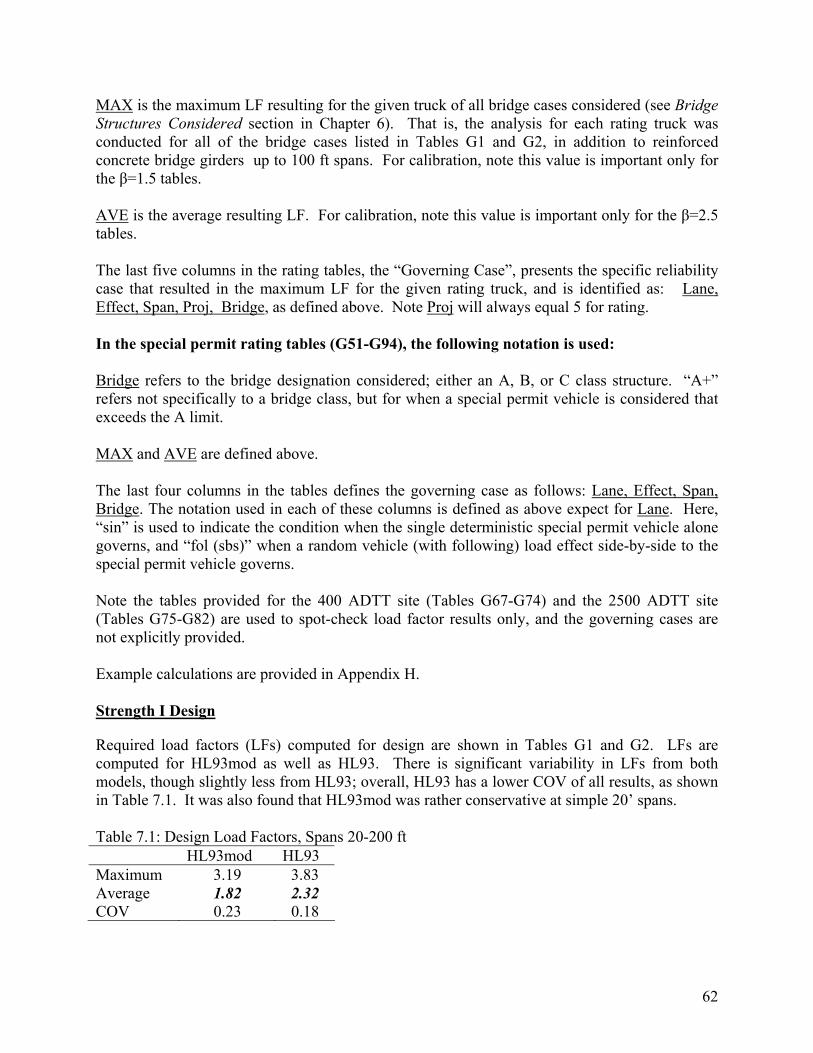
62

MAX is the maximum LF resulting for the given truck of all bridge cases considered (see Bridge Structures Considered section in Chapter 6). That is, the analysis for each rating truck was conducted for all of the bridge cases listed in Tables G1 and G2, in addition to reinforced concrete bridge girders up to 100 ft spans. For calibration, note this value is important only for the β=1.5 tables. AVE is the average resulting LF. For calibration, note this value is important only for the β=2.5 tables. The last five columns in the rating tables, the “Governing Case”, presents the specific reliability case that resulted in the maximum LF for the given rating truck, and is identified as: Lane, Effect, Span, Proj, Bridge, as defined above. Note Proj will always equal 5 for rating. In the special permit rating tables (G51-G94), the following notation is used: Bridge refers to the bridge designation considered; either an A, B, or C class structure. “A+” refers not specifically to a bridge class, but for when a special permit vehicle is considered that exceeds the A limit. MAX and AVE are defined above. The last four columns in the tables defines the governing case as follows: Lane, Effect, Span, Bridge. The notation used in each of these columns is defined as above expect for Lane. Here, “sin” is used to indicate the condition when the single deterministic special permit vehicle alone governs, and “fol (sbs)” when a random vehicle (with following) load effect side-by-side to the special permit vehicle governs. Note the tables provided for the 400 ADTT site (Tables G67-G74) and the 2500 ADTT site (Tables G75-G82) are used to spot-check load factor results only, and the governing cases are not explicitly provided. Example calculations are provided in Appendix H. Strength I Design

Required load factors (LFs) computed for design are shown in Tables G1 and G2. LFs are computed for HL93mod as well as HL93. There is significant variability in LFs from both models, though slightly less from HL93; overall, HL93 has a lower COV of all results, as shown in Table 7.1. It was also found that HL93mod was rather conservative at simple 20’ spans. Table 7.1: Design Load Factors, Spans 20-200 ft HL93mod HL93 Maximum 3.19 3.83 Average 1.82 2.32 COV 0.23 0.18

63

In all LF tables in the Appendix, both the average as well as the maximum LF for each case is given. The average result is used to determine appropriate LFs to meet the target index. However, the maximum is presented for interest and comparison. The average is computed from the results obtained by taking the maximum (governing) LF required from either a single lane loaded (fol) or two lanes loaded for each bridge case. Moreover, when the average LF is computed corresponding to the target index, note that this average is based on the mean from the number of bridge cases considered. In this regard, steel, prestressed concrete, and spread box beam bridges are equally weighted, while side-by-side box beams have fewer cases and are correspondingly weighted with a lower fraction (0.4) relative to the other cases. When reinforced concrete is considered for rating cases, it is also weighted at a slightly lower fraction of 0.80 relative to the others. When 300-400’ spans are considered, a higher LF is required, with an average of 2.24 with HL93mod. Note that for these spans, since the HL93 truck load governs over the 60k axle associated with HL93mod, the average LF associated with HL93 is simply 2.24 x 1.2 = 2.69. This significant increase is not due to the HL93 design load inaccurately modeling the load effect at longer spans; in fact, it is slightly conservative as span length increases beyond 200’, as shown in Table 7.2. Rather, the increase relative to the 20-200’ spans is primarily due to the conservatism of the model at lower spans, where the lower LFs generally occur from spans 20-50’. Removing these spans from the average taken in the 300-400’ case results in a higher required LF. Table 7.2. Comparison of HL93 and maxL

* maxL based on a 75 year projection for all vehicles, 1-lane (following) moment.

Although the maximum design LFs for the worst case bridge appear large, the results are not unexpected, based on the results presented in NCHRP 683. For example, based on WIM data from several states, NCHRP 683 presents approximate new design live load factors (for LRFD), calculated as a function of “r” values, which represent the ratio of the mean maximum load effect found from the projected WIM data to the mean maximum load effect used in the AASHTO

64

LRFD calibration. These r values are then multiplied by the existing LRFD live load factor to determine appropriate new live load factors. In the NCHRP report, it was found that the maximum (governing) r-values for the worst-case load effect were approximately 2.20, 2.05, 1.99, 1.88, 1.78, 1.79, 1.80, and 1.82, for span lengths of 20, 40, 60, 80, 100, 120, 160, and 200’, respectively. Multiplying these by the existing LRFD live load factor of 1.75 results in final live load factors ranging from 3.12-3.85, values nearly the same as the maximum design live load factors determined in this study (see Table G1). With regard to average LF, it was found that in Florida, the live load factor required an increase to 2.37 to meet the target index of 3.5. Note this is nearly the same as the value found above for HL93 in this study (2.32) as well. Strength I (Legal Load) Rating

Legal load rating results are given for a pool of sites with 1000 ADTT, ADTT ≥ 5000, as well as two individual sites; 2029 (~400 ADTT) and 5059 (2500 ADTT) for verification. These results are presented in Tables G3-G34 in Appendix G. For rating analysis, all bridge configurations (the same as in design, but with the addition of reinforced concrete bridges as well) were considered for each of 28 MI legal trucks. LFs for each bridge case considered are not given due to the extent of the output data (approximately 930 reliability indices computed per method (LFR and LRFR), per truck). Rather, in the tables, for each legal truck, two results are given: the maximum governing LF from all of the bridges considered, along with the governing bridge case, as well as the average from all bridges. The analysis is conducted for both cases of the target reliability index of 2.5 and the minimum of 1.5. For the rating target index of 2.5, the average value shown is important; the maximum value is provided for interest and to identify the worst-case considered, but is not used in the calibration. For the rating minimum index of 1.5, the minimum is required rather than the average. For the ADTT 1000 case, spans from 20-200’, it was observed that at the rating target reliability level of 2.5, for LFR, the governing case for all trucks was a single lane load effect, simple or continuous span of 200’, spread box beam bridge with spacing at 4’. This governing case generated average LFs from 3.34 (truck 1) to 1.31 (truck 22). The reason for this governing case is that the spread box beam DF is unconservative relative to the LRFD (analysis) DF for this structure (for this case, the DF for AASHTO Standard = 0.45; the DF for LRFD = 0.49). This is not surprising, as the AASHTO Standard DF formulas are known to provide lower DF results as compared to LRFD at low girder spacing. For LRFR, all governing cases were a single lane effect (fol); most are simple shear at 200’ span for a prestressed concrete girder spaced at 4’, though several were side-by-side box beam members at 20’ span in continuous shear. LRFR LFs are not only lower than LFR, but also more consistent. This improved consistency is expected since the DF used in the reliability analysis to distribute actual load effects (with the addition of appropriate bias factor) is same as that used in LRFR. Average LFs required to meet target ranged from approximately 2.43 (truck 1) to less than 1. One reason that LFR produces higher LFs is that many of the governing cases are with continuous spans; in LRFR, a more conservative 2-truck load model is used for continuous spans which increases bridge rating capacity in these cases, while LFR only uses one truck.

65

Note that although the single lane load effect is generally what was found to govern LF overall, this does not mean that single lane traffic produced a higher load effect than the side-by-side effect in every bridge case considered; in fact, in many cases side-by-side produced a greater result. These cases, however, did not produce the highest load factor overall and thus do not appear in the summary tables. That is, a bridge case with a different span, load effect, and girder type and spacing than what governed overall may have had a larger side-by-side load effect than single lane; but since this case produced a lower load factor than what governed overall, it does not appear in the table. When the minimum index imposed on all cases of 1.5 is considered, rather than an average requirement of 2.5, very high LFs result; from 5.99 for truck 1 to 1.70 for truck 17. Governing cases are simple shears at 200’ span, and typically for steel girders spaced at 4’. For LRFR, governing cases are generally the same as with LFR. Note that the maximum LF required in each case is significantly higher than the average. This indicates that one specific (or a few similarly high cases), worst-case result is governing the required LF. This is an unfortunate finding, as this indicates significant inconsistency among the different cases; for the few worst-case results to meet the minimum target, the majority of structures will be significantly penalized unnecessarily. As also found by Sivakumar et al. (2011), it is the minimum reliability index imposed which governs over the target in every case considered from spans 20-200’. For longer spans, however, the target index often governs. Which of these reliability limits governs depends on how close the rating model is to how the actual loads are distributed to the girder; the greater the discrepancy, the more likely that the minimum index will govern with extreme cases. For the longer spans, many of the extreme cases that appear for shorter spans are eliminated, producing required load factors from the two reliability limits that are much closer together. The extreme cases are reduced in the longer spans because no approximate girder distribution factor formulas (as with LFR) or varying load distribution bias factors are used (for both LFR and LRFR), which are not available for non-girder bridges. That is, as discussed in Chapter 6, it is assumed that the actual distribution factor on a long span member is identical to that used in the design/rating procedure. Distribution factor discrepancies were the cause of many of the extreme cases for the shorter spans which caused the minimum reliability level to control. A discussion of why the governing LFs are so high is given below. For spans from 300-400’, when the target index of 2.5 is considered, for LFR, it was found that for longer spans, LFR has significantly lower LFs than LRFR. This is due to the requirement in LFR to apply a train of vehicles in the lane (alongside a single vehicle in the adjacent lane), which has a tremendous impact on the rating load effect. In all cases, the governing case is a single lane load effect (i.e. in terms of the projected load effects on the span), for simple shear at the 300’ span. Prestressed concrete LFs are higher than steel in every case for the 300-400’ spans due to a higher variance of shear resistance (COV for PC shear resistance = 1.14; COV for steel shear resistance = 0.105). For LRFR, the same case as for LFR governs; the 300’ span simple shear. When the minimum index of 1.5 is considered, it was found that for LFR, LF ranges from 2.31 for truck 1 to 1.07 for truck 17. For LRFR, much higher LFs were required, ranging from 7.06

66

for truck 1 to 2.75 for truck 22. For both LFR and LRFR, the same cases governed as for when the target of 2.5 was considered. Considering the 5000 ADTT sites, overall trends are similar to the 1000 ADTT results, but with about 20% higher LFs required. Cases that governed for the 1000 ADTT results are identical for LFR, while for LRFR, several governing cases switched from the previous PC beam spaced at 4’ with 200’ span to a spread box beam member with 12’ spacing and 20’ span. For 300-400’ spans, governing cases did not change from the 1000 ADTT case, and LFs increased by approximately 34%. To illustrate why the governing LF is very high, consider an example case in LRFR with truck 1, which has the highest LF in this case of 4.22 for the minimum reliability index of 1.5 This governing case is a single lane, simple shear effect at 200’ span for a steel beam spaced at 4’. The simple reason for the high LF is a large applied load relative to the rating truck. For this case, the projected mean maximum load effect is 310 kips (which perhaps may occur in the case of several very heavy following vehicles on the 200’ span), but the rating truck nominal shear on this span length is calculated at 38 kips; approximately 1/8th (!) of the mean maximum load projection. A higher capacity rating truck will have a correspondingly lower LF. For example, if the HL93mod load were used to rate this case, with a nominal shear at this span length of 186k, the required LF drops to 1.14. Similar observations can be made for the other very high LFs as well. When site 2029 (~400 ADTT) was considered, as expected, LFs fall below the ADTT 1000 sites, with similar overall trends. On average, LFs are reduced by approximately 10% for 20-200’ spans and approximately 11-12% for 300-400’ spans. However, these reductions are not uniform. Considering site 5059 (~2500 ADTT), LF values fell between those calculated for the 1000 and 5000 ADTT sites, but were much closer to the lower values of ADTT 1000, experiencing a 1% increase on average over the ADTT 1000 values for both LFR and LRFR, but average of 15% less than the 5000 ADTT site for LFR and an average of 19% less when LRFR is considered. Therefore, it seems reasonably conservative to linearly extrapolate LFs between sites for ADTT 2500. Overall, it was found that the average LFs at the minimum reliability level of 1.5, for both 5000 and 1000 ADTT sites, were roughly at the level of the existing MDOT LFs for many vehicles. However, imposing the minimum reliability index of 1.5 on all cases resulted in significantly higher LFs. To better understand the pattern of variation of LFs, Figures G1-G20 in the Appendix present the LF required (for either the 1 or 2-lane load effect, whichever governed) for each bridge type and load case for two example legal vehicles (numbers 2 and 23) to meet the minimum reliability index of 1.5 for 5000 ADTT, for spans from 20-200 ft. Individual cases are identified by the label: “(load effect) (span)-(girder spacing)”. For example, “Ms 50-06” refers to simple moment for 50 ft span, 6 ft girder spacing. As shown in the figures, shears at the longer spans and smaller girder spacings tend to govern overall LF for most bridge types for vehicle 2, while

67

shears across shorter spans and smaller girder spacings tend to govern for vehicle 23. As expected, differences between governing and average LFs appear to be wider for LFR than LRFR, due to the different accuracy of the distribution factors used for rating. Note that the required LFs reported in the recommendations (Chapter 8, Table 8.1) to meet the minimum index of 1.5 represent the maximum LF of any case. For example, the required LF for vehicle 2 at 5000 ADTT for LFR is reported as the maximum LF of any value in Figures G1-G5 (and is shown to be 5.66 for case Vs 200-04 for steel, in Figure G1). This value can also be found in Table G12 with the same governing case identified. Because relatively high LFs are spread throughout multiple spans and bridge types, it is not clear how LFs could be practically reduced by eliminating rare cases. For example, for LFR, removing all of the 4 ft girder spacing shear checks for all bridge types for would reduce the required LF for vehicle 2 from 5.66 to 4.28; the remaining governing case is then Vs 200-06 for steel. Eliminating all 200 ft shear checks for all bridge types would reduce the required LF from 5.66 to 4.63 (remaining governing case Vs 100-04 for CS). Eliminating shear checks for both 4 ft girder spacing and all shear checks for 200 ft spans would reduce the required LF from 5.66 to 3.75 (remaining governing case Vs 100 for side-by-side box beams). Eliminating all shear checks completely would reduce the required LF from 5.66 to 3.73 (remaining governing case Mc 50-04 for spread box beams) Strength II Rating, Routine Permits

Routine permit results are presented in Tables G35-G50 in the Appendix. For the 20-200’ spans, continuous shears control for LFR and LRFR for almost all cases, generally at the shortest span lengths (20’ for most vehicles). Considering the 1000 ADTT sites, there is significant variation in resulting LFs, but overall, routine permit LFs are about 50% higher on average than legal factors for LFR, but lower than the corresponding legal factors for LRFR. This is primarily because LFR uses a 2 lane DF for legal load assessment but a 1 lane DF for permit load assessment; Rn is correspondingly lower for permit load rating. For LRFR, significant variation also exists from case to case, but overall, routine permit loads have the same average LFs (averaged across all trucks) as the legal rating factors. When the 300-400’ spans are considered, for LFR, LFs are higher for permit rating than for legal rating. This is because not only is a single lane DF used for permit loads (as opposed to a 2 lane DF for legal load rating), but a single vehicle is used (as opposed to the vehicle train for legal load rating). These changes significantly reduce the bridge rating capacity. In contrast, for LRFR, LFs for permit rating are significantly lower than for legal load rating. In LRFR, the load rating methods for permit and legal loads are not identical but closely similar. However, for permit rating, the routine permit vehicle pool results in significantly lower load effects at higher span lengths than the general vehicle pool; this is due to restricting the upper vehicle weights used in the routine vehicle load projection, as described in Chapter 6. This narrower band of vehicles also lowers COV of the resulting load, further increasing reliability. In the case of LFR, however, this lower load effect is outweighed by the changes in the rating procedure. For the 5000 ADTT sites, the overall trends from the 1000 ADTT sites are followed. Here, continuous shear controls almost all cases, which are a spread box beam member spaced at 4’ for LFR and a reinforced concrete member spaced at 4’, or a side-by-side box beam for LRFR.

68

Average LFs are only slightly higher, however (by about 2% for both LRFR and LFR), than the 1000 ADTT case. For LRFR, LFs resulting from the minimum reliability index limit case are within the range of most exiting MDOT legal LFs. For 300-400’ spans, single lane continuous moment governs with steel structures rated with LFR for all cases when considering the target index of 2.5; whereas simple shear governs all corresponding cases in LRFR. For prestressed concrete structures, 400’ shears govern all cases. When considering the minimum reliability limit of 1.5, 300’ simple shears govern all cases of LFR as well as LRFR, for both steel and PC structures. Sites 2029 (~400 ADTT) as well as 5059 (~2500 ADTT) cannot be evaluated for routine permit comparison, as both had an insufficient number of routine permit crossings for accurate analysis. As discussed in Chapter 6, it was desired to check whether routine permit load effects would be adequately accounted in rating for using legal vehicles and their corresponding LFs. For 5000 ADTT and above traffic volumes, this is true for LRFR for all cases (comparing the LFs in Tables 8.1-8.4, the governing legal LF is always higher than the routine permit factor for the same vehicle). However, note that slightly different procedures are used in LRFR to rate capacity for legal and routine permit loads, as described in Chapter 6. For 1000 ADTT in LRFR, and for both 1000 and 5000 ADTT in LFR, some routine permit factors are larger than the legal LFs (see Tables 8.1-8.4). However, for LFR, a 1-lane distribution factor is used for routine permit rating and a 2-lane factor is used for legal rating, so the LFR routine permit capacity is biased to produce a higher LF than legal for the same vehicle in the rating procedure. Even in the case of LRFR, the routine permit checking procedure is not identical to the legal load checking procedure, as noted in Chapter 6. However, if the rating procedures were kept the same; for example, by changing the routine permit rating procedure to exactly match the legal rating procedure, then in most load effects considered, legal loads would generate higher LFs, as routine permit load effects are usually less than those for legal loads (as explained earlier in the report). However, exceptions exist. These can be seen in the load projection Tables (F6-F9), by comparing the values of the three load parameters presented between the legal load and routine load projections for the same case: mLmax, Vproj, and Vsite. When any of these three values are increased, without an off-setting reduction in the remaining two values, then LF must also be increased to maintain the same level of reliability. Table 7.3 presents the specific load effect cases where any one of these three values in the routine permit load projection is higher than the corresponding value in the legal load projection (same for 1000 as well as 5000 ADTT).

69

Table 7.3. Routine Permit Load Effects Potentially Greater than Legal Load Effects

In many of the cases shown in Table 7.3, it may be that an increase in one of the values of mLmax, Vproj, or Vsite is sufficiently offset by a decrease in one of the remaining values to avoid generating a routine permit LF higher than the corresponding legal LF (assuming the rating procedure is kept identical for legal loads and routine permits). As the relationship among mLmax, Vproj, and Vsite and reliability index is not proportional, this cannot be determined based on the load values alone; the only way this can be checked conclusively is by recalculating routine permit load factors. Tables G95-G110 present the corresponding LFs. The LFs shown in these tables were determined by evaluating the routine permit load effects using the legal load rating procedure. This allows direct comparison between the legal load LFs and routine permit LFs; i.e. the only factor contributing to a difference in the results is the difference in projected legal and routine permit loads shown in Appendix F. As can be seen within the long-span Tables G97, 98, 101, 102, 105, 106, 109, and 110, all long span routine permit LFs are lower than the corresponding legal load LFs (Tables G5, 6, 9, 10, 13, 14, 17, 18). Moreover, as single lane effects control in all of the tables, the two lane cases shown in Table 7.3 are not relevant. This leaves only the first 7 rows of single lane load effects in Table 7.3 which are a potential concern for the shorter (20-200 ft) spans (i.e. where routine permit loads may possibly have higher load factors than legal loads within the legal rating system). Unfortunately, as shown in Tables G95, 96, 99, 100, 103, 104, 107, and 108, the minimum reliability index check dominates, as usual, and there are numerous cases where routine permit load factors are higher than the corresponding legal load factor (Tables G96, 100, 104, and 108, as compared to the legal load values in Tables G4, 8, 12, and 16 ). As shown in Tables G96, 100, 104, and 108, the governing load effect is usually Vc 20 (continuous shear, 20 ft span) for most trucks. Eliminating this particular load effect would not necessarily improve results, however, as the other single lane load effects shown in Table 7.3 would then govern. Therefore, although in many cases it is

70

acceptable, in all cases it is not reasonable to evaluate permit loads using legal LFs. These cases are not bridge dependent but load effect dependent, as shown in the first 7 rows of Table 7.3. Strength II Rating, Special Permits

Special Permit Crossing With Other Traffic Special permit results are presented in Tables G51-G82 in the Appendix. Here, it can be seen for the 1000 ADTT case, with target index of 2.5 considered with 20-200’ spans, for both LFR and LRFR, the average LF needed to meet the average reliability target were slightly less than 1. When the minimum index is considered for any case, however, LFR required LFs of approximately 1.4 for all bridges (A, B, C, and above A), where the governing case was 20’ simple span moment, for spread box beams at 4’ spacing. LRFR required minimum LFs of approximately 0.93 for all bridges, with governing cases of spread boxes spaced at 12’. The higher LFs required of LFR result from an unconservative LF for 4’ spaced spread box beams, which is nearly half that specified by the LRFD DF expression. For the 300-400’ spans, the differences in DFs are eliminated and the LFs are much closer, where LFR has only slightly larger factors. For LFR, LFs from 1.5-1.9 are required to meet the target index (where prestressed concrete in shear governs), while values from 1.1-1.4 are required of LRFR. The minimum reliability index is met by both LFR and LRFR with LFs less than 1. For the 5000 ADTT sites, trends are similar to the 1000 ADTT results, with governing cases nearly identical. Note that when the single permit vehicle alone controls (i.e. case “sin”), LFs are identical for all sites, as the random alongside vehicle effect does not govern. For these cases (which occur only in steel structures), LFs are only slightly (1-2%) higher than for 1000 ADTT. As expected, site 2029 has lower required LFs than the 1000 ADTT site, but with significant differences only in a few cases. LFs for site 5059 are nearly identical to 5000 ADTT values. Special Permit Escorted Across Bridge Results for an escorted special permit are given in Tables G83-G90. In this case, the rating bridge capacity is reduced by lowering impact factor to 1.05. It is assumed that the same factor will be applied during the rating process to represent the crawling speed vehicle as it is escorted across the bridge. Here, the results are identical for all sites, as no site load data is considered, as no random vehicles load the bridge while the special permit vehicle crosses. In this case, maximum LFs required from LFR are approximately 1.6 for 20-200’ structures, and slightly over 1 for LRFR. The primary reason for this difference is discussed above. For 300-400’ span structures, required LFs range from about 1.6-1.8 in LFR and are about 1.5 for LRFR.

71

CHAPTER 8: RECOMMENDATIONS

Recommended Live Load Factors As discussed previously, because there is significant variation in the required LF from one bridge case to another, generally, a small selection of extreme cases controls and sets the maximum LF across the entire set of bridges considered. This is particularly so for rating. For practical implementation, it is desirable to use the same LFs for all bridge cases or for a broad set of cases. To do this effectively and minimize penalization to non-governing structures, it is recommended that the rating procedure is formally optimized. That is, an optimization can be conducted where design variables are taken as rating procedure variables, such as how rating loads are applied and what distribution factors are used. The optimization process would then best design the rating procedure to produce the lowest discrepancies in reliability among the different bridge cases for a given LF, while under the constraints that no case falls below the minimum required reliability level, or is potentially too high. Less ideal approaches than this optimization procedure are discussed below. Live Load Factors for Design Because it was found that the AASHTO LRFD HL93 provides a lower variance in LF results, it is recommended to replace HL93mod with HL93, with a LF=2.3 for girder bridges. This will allow an average reliability index of approximately 3.5 across all girder bridge types. For longer span, non-girder bridge structures, it is similarly recommended to use HL93 with a LF=2.7, which will allow these structures to meet an average target reliability index of 3.5. Note that at these span lengths, the 60k axle of HL93mod does not govern, and HL93mod is simply a 1.2 multiple of HL93. Although variation in the results exists beyond that seen in the AASHTO LRFD code calibration, the results appear somewhat reasonably consistent. For the 20-200’ spans, a solution to further moderate the varying range of reliability indices across bridge cases considered is not clear, as with reference to the HL93 load, long span simple shears tend to have the highest LFs required, while continuous moments and shears tend to have the lowest LFs. Live Load Factors for Rating Due to the very wide variation among the different truck cases and bridge spans, the ideal case to maintain consistency in reliability as well as to avoid unnecessary traffic restrictions would be to apply individual LFs for each truck for each bridge case. However, given that hundreds of bridge cases were explored, this may become impractical. Therefore, several possibilities exist. The most conservative route, and that used in the MBE recalibration, would be to use the governing LF from either the average for the target index of 2.5 or the maximum for the minimum index of 1.5, for each rating truck. These results are summarized below, in Tables 8.1-8.6. The governing index for each case (from the target or minimum reliability limit) is given in boldface. Note that these LFs are only applicable when used in conjunction with the rating procedures as described in Chapter 6 (i.e. the default rating procedures per LFR and LRFR). It is further recommended that LFs be limited to values ≥ 1.0 (i.e. LFs in the tables less than 1.0 be raised to 1.0). However, the magnitudes of most resulting LFs in Tables 8.1-8.6 are

72

very high relative to current MDOT practice. Thus, it may not be feasible for MDOT to apply these LFs to all structures. As such, the optimization approached summarized above is particularly recommended for rating. Note that NCHRP 20-07(285), based on a procedure similar to that which was used in this report, lower LFs were generally developed than shown here. There are three main reasons for these differences: Different loads. Projected Michigan loads are generally higher, sometimes substantially, than those found in NCHRP 20-07(285), which used sites from California, Florida, Indiana, Mississippi, New York, and Texas. For example, considering a five year legal load projection for 5000 ADTT sites, the ratio of Michigan to NCHRP 20-07(285) moment averaged across all sites ranged from 1.03-1.67 (see Table 8.7). Comparing the site averaged Michigan moment to the moment found from the single highest NCHRP 20-07(285) site, the ratio peaked at 1.27 (100 ft span). Site averaged shear ratios ranged from 0.99-1.37. Different vehicles. NCHRP 20-07(285) used AASHTO legal vehicles rather than the 28 Michigan legal vehicles. Many of the Michigan legal vehicles produce significantly lower load effects than the AASHTO legal vehicles, requiring higher LFs for the same reliability level. Different project scopes. NCHRP 20-07(285) used data from 6 WIM sites totaling 11.8 million vehicles, all outside of Michigan, to construct its live load database, while this project used data from 20 WIM sites all inside Michigan with a total of approximately 66 million vehicles. Moreover, although the same range of girder spacings were analyzed (4-12 ft), NCHRP 20-07(285) considered spans no longer than 200 ft, while this study included spans up to 400 ft. For the spans, NCHRP 20-07(285) calculated simple load effects (moment and shear) only, while this study included both simple and continuous span load effects. Another difference is that NCHRP 20-07(285) included reinforced concrete girders, steel girders, and prestressed concrete girders, while this study used those girder types as well as prestressed concrete side-by-side and spaced box beam girders. Thus, in terms of different cases considered, the scope of this study is somewhat wider that that of NCHRP 20-07(285), and the additional cases considered often governed LFs (longer spans, box beams, continuous load effects). The potential impact of implementing any changes in current MDOT LFs on current truck traffic can be estimated. This can be done by multiplying the load effects of currently legal vehicles in the WIM data by the ratio of: (new LF / current LF). Those vehicles that then produce load effects that exceed the (unfactored) current legal load effect envelope may encounter route restrictions with the new LFs. Note that the “5000 ADTT” in the tables also applies for sites with ADTT > 5000 ADTT, as various sites used to develop the LFs for that case have ADTT > 5000. For sites with ADTT between 1000 and 5000, an interpolation of LFs is recommended. For sites below 1000 ADTT, it is recommended use the values for 1000 ADTT. In lieu of using the LFs above, another option is to consider a modification of the reliability targets. If the existing level of reliability on MDOT bridges is deemed reasonable, the reliability

73

targets could be lowered to better represent existing bridge reliability levels. This was conducted in New York to avoid increasing existing LFs beyond a level which was deemed practical (Sivakumar et al. 2011). It is further recommended that a switch to LRFR is made. This will provide greater consistency in reliability, primarily at lower girder spacing cases, by using the AASHTO LRFD distribution factor expressions in place of the generally less accurate AASHTO Standard expressions. Table 8.1. Governing Load Factors, Legal Load Rating, Spans 20-200 ft.

74

Table 8.2. Governing Load Factors, Legal Load Rating, Long Spans.

75

Table 8.3. Governing Load Factors, Routine Permit Rating, Spans 20-200 ft.

76

Table 8.4. Governing Load Factors, Routine Permit Rating, Long Spans.

77

Table 8.5. Governing Load Factors, Special Permit Rating.

Table 8.6. Governing Load Factors, Special Permit (Escorted) Rating.

Table 8.7. Simple Span 1-Lane, 5 Year Mean Maximum Live Load Ratios (MI/NCHRP), 5000 ADTT.

MI/NCHRP Load Effect Ratio Load Effect 20’ Span 100’ Span 200’ Span Moment (average) 1.03 1.67 1.50 Moment (max NCHRP) 0.74 1.27 1.26 Shear (average) 0.99 1.34 1.37

78

REFERENCES AASHTO LRFD Bridge Design Specifications, 5st ed. American Association of State Highway and Transportation Officials, Washington, D.C., 2010. AASHTO Manual for Bridge Evaluation, 2nd ed. American Association of State Highway and Transportation Officials, Washington, D.C., 2011. AASHTO Manual for Condition Evaluation and Load and Resistance Factor Rating (LRFR) of Highway Bridges, American Association of State Highway and Transportation Officials, Washington, D.C., 2003. AASHTO Manual for Condition Evaluation of Bridges, American Association of State Highway and Transportation Officials, Washington, D.C., 1998. Ang, A. H-S. and Tang, W.H. “Probability Concepts in Engineering.” Wiley, 2007. Au, S.K. and Beck, J.L. “Estimation of small failure probabilities in high dimensions by subset simulation.” Probabilistic Engineering Mechanics, Vol. 16, No. 4, pp. 263-277, 2001. Au, S.K., Ching, J., and Beck, J.L., “Application of subset simulation methods to reliability benchmark problems.” Structural Safety, Vol. 29, No. 3, pp. 183-193, 2007. Ayyub, B.M., and Haldar, A. “Practical Structural Reliability Techniques.” Journal of Structural Engineering, ASCE, Vol. 110, No. 8, pp. 1707-1724, 1984. Breitung, K. “Asymptotic Approximations for Multinormal Integrals.” Journal of Engineering Mechanics, ASCE, Vol. 110, No. 3, pp 357-366, 1984. Bruls A, Croce P, Sanpaolesi L, Sedlacek O. ENV1991 - Part 3: traffic loads on bridges; calibration of load models for road bridges. In: Proceedings of IABSE colloquium, Delft, The Netherlands: IABSE-AIPC-IVBH; pp. 439-53, 1996. Bucher, C.G. and Bourgund, U. “Fast and efficient response surface approach for structural reliability problems.” Structural Safety, Vol. 7, No. 1, pp. 57-66, 1990. Chen, X. and Lind, N.C. “Fast Probability Integration by Three-Parameter Normal Tail Approximation.” Structural Safety, Vol. 1, pp. 269-276, 1983. Cheng, J. and Li, Q.S. “Application of the response surface methods to solve inverse reliability problems with implicit response functions.” Computational Mechanics, Vol. 43, No. 4, pp. 451-459, 2009. Croce, P. and Salvatore, W. "Stochastic model for multilane traffic effects on bridges.” ASCE Journal of Bridge Engineering, Vol. 6, No.2, pp. 136-143, 2001. Curtis, R. and Till, R. "Recommendations for Michigan Specific Load and Resistance Factor Design Loads and Load and Resistance Factor Rating Procedures." MOOT Research Report R-1511, April 2008. Data Collection Guide for SPS WIM Sites, 1st ed. Federal Highway Administration, Turner- Fairbank Highway Research Center Pavement Performance Division, Virginia, 2001. Dawe P. Research perspectives: traffic loading on highway bridges. London: Thomas Telford, 2003. Der Kiureghian, A., Lin, H.Z., and Hwang, S.J. “Second-Order Reliability Approximations,” Journal of Engineering Mechanics, ASCE, Vol. 113, No. 8, pp. 1208-1225, 1987. Eamon, C. and Charumas, B. “Reliability Estimation of Complex Numerical Problems using Modified Conditional Expectation Method,” Computers and Structures, No. 89, pp. 181- 188, 2011.

79

Eamon, C., Thompson, M., and Liu, Z. “Evaluation of Accuracy and Efficiency of some Simulation and Sampling Methods in Structural Reliability Analysis,” Journal of Structural Safety, Vol. 27 No. 4, pp. 356-392, 2005. ECI. Eurocode 1: actions on structures. Part 2: Traffic loads on bridges. Brussels: European Standard EN 1991-2:2003: European Committee for Standardization, TC250, 2003. Elicegui, M., Stefonowicz, T., and Severns, D. “Loads and Load Factors." NDOT Structures Manual, Chapter 12, Nevada Department of Transportation, 2008. Elkins, L., and Higgins, Ch. “Development of Truck Axle Spectra from Oregon Weight-in- Motion Data for use in Pavement Design and Analysis." FHWA, Report no. OR-RD-08- 06, Oregon Department of Transportation and Federal Highway Administration, 2008. Engelund, S. and Rackwitz, R. “A benchmark study on importance sampling techniques in structural reliability, Structural Safety, Vol. 12, No. 4, pp. 255-276, 1993. Fiessler, B., Neumann, H.J., and Rackwitz, R. “Quadratic Limit States in Structural Reliability.” Journal of Engineering Mechanics, ASCE, Vol. 1095, No. 4, pp. 661-676, 1979. Folwell, M. and Stephens, Jerry. "System for Processing and Analyzing WIM and AVC Data." FHWA, Report no. MT-97/8117-3, Montana Department of Transportation 1997. Fu, G. and Hag-Elsafi, O. "Vehicular Overloads: Load Model, Bridge Safety, and Permit Checking." ASCE Journal of Bridge Engineering, Vol. 5, No.1, pp. 49-57, 2000. Fu, G., Feng, J., Dekelbab, W., Moses, F., Cohen, H., Meliz, D., and Thompson, P. "Effect of Truck Weight on Bridge Network Costs." NCHRP Report 495. Washington, D.C., Transportation Research Board, 2003. Fu, O. and Van de Lindt, 1. "LRFD Load Calibration for State of Michigan Trunkline Bridges." MDOT Research Report RC-1466, August, 2006. Fu, O. and You, J. "Truck Loads and Bridge Capacity Evaluation in China." ASCE Journal of Bridge Engineering, Vol. 14, No.5, pp. 327-335, 2009. Ghosn, M. "Development of Truck Weight Regulations Using Bridge Reliability Model." ASCE Journal of Bridge Engineering, Vol. 5, No.4, pp. 293-303, 2008. Ghosn, M. and Moses, F. "Reliability Calibration of Bridge Design Code.” Journal of Structural Engineering, Vol. 112, no. 4, 1986. Ghosn, M., Sivakumar, B., and Miao, F. "Load and Resistance Factor Rating (LRFR) in NYS, Volume II, Final Report." NYSDOT Report C-06-13., 2011. Ghosn, M., Sivakumar, B., and Moses, F. "Modeling maximum live load effects on highway bridges." Proceedings from the First International Symposium on Live-Cycle Civil Engineering, Varenna, Italy, June, pp. 335-341, 2008. Ghosn, M., Sivakumar, B., and Moses, F. "Using weigh-in-motion data for modeling maximum live load effects on highway bridges.” Proceedings of the Fifth International IABMAS Conference, Philadelphia, USA, July, 2010. Gindy, M., and Nassif, H.H. "Multiple presence statistics for bridge live load base on weigh-in- motion data." Transportation research board 86th annual meeting, Washington, D.C., 2006. Gomes, H. M. and Awruch, A. M. “Comparison of response surface and neural network with other methods for structural reliability analysis.” Structural Safety, Vol. 26, No. 1, pp. 49-67, 2004. Hohenbichler, M., Gollwitzer, S., Kruse, W., and Rackwitz, R. “New Light on First- and Second-Order Reliability Methods.“ Structural Safety, Vol. 4, pp. 267-284, 1987.

80

Iman, R.L., and Conover, W.J. “Small Sample Sensitivity Analysis Techniques for Computer Models, with an Application to Risk Assessment.” Communications in Statistics: Theory and Methods. Vol. A9 No. 17, pp. 1749-1842, 1980. Karamchandani, A., Bjerager, P., and Cornell, A.C. “Adaptive Importance Sampling.” Proceedings, International Conference on Structural Safety and Reliability (ICOSSAR), San Francisco, CA., pp. 855-862, 1989. Kwon, O-S, Kim, E., Orton, S, Salim, H., and Hazlett, T. "Calibration of the Live Load Factor in LRFD Design Guidelines", MODOT Report ORI1-003, Sept. 2010. Lee, C.E. and Garnet, J.E. “Collection and Analysis of Augmented Weight-in-Motion Data." Center for Transportation Research Bureau of Engineering Research, the University of Texas at Austin, Report no. 987-8, 1996. Lee, C.E. and Souny-Slitine, N. “Final Research Findings on Traffic-Load Forecasting Using Weight-in-Motion Data." Center for Transportation Research Bureau of Engineering Research, the University of Texas at Austin, Report no. 987-7, 1998. Lu, Q., Harvey, J., Le, J., Quinley, R., Redo, D., and Avis, J. “Truck Traffic Analysis using Weigh-In-Motion (WIM) Data in California." University of California, Berkeley Institute of Transportation Studies, Pavement Research Center, 2002. MDOT Bridge Analysis Guide, 2005 Ed, with 2009 Interim Update, Parts 1 and 2. MDOT Construction and Technology Support Area, 2009. MDOT Maximum Legal Truck Loadings and Dimensions, T-1. MDOT, 2011. Miao, T.J. and Chan. T.H.T. “Bridge live load models from WIM data.” Engineering Structures, Vol. 24, No. 8, pp. 1071-1084. 2002. Monsere, L., Higgins, Ch. and Nichols, A. “Application of WIM Data for Improved Modeling, Design, and Rating." Oregon Transportation Research and Education Consortium, Oregon Department of Transportation, 2011. Moses, F. "Calibration of load factors for LRFR bridge evaluation." NCHRP Report no. 454, Washington, D.C., Transportation Research Board, 2001. Moses, F. and Ghosn, M. "Instrumentation for Weighing Trucks-In-Motion for Highway Bridge Loads." Final Repol1, FHWAfOH-83-001 to Ohio DOT, Case Western Reserve University, August, 1983. Nowak, A.S. "Calibration of LRFD Bridge Design Code." NCHRP 368, Washington, D.C., Transportation Research Board, 1999. Nowak, A.S. “Calibration of LRFD Bridge Code.” Journal of Structural Engineering. Vol. 121, No. 8, pp. 1245-1251, 1995. Nowak, A.S. “Live load model for highway bridges.” Structural Safety, Vol. 13, pp. 53-66, 1993. Nowak, A.S., Lutomirska, M., and Sheikh Ibrahim, F.I. "The development of live load factors for long span bridges.” Bridge Structures, Vol. 6, No. 1, pp. 73-79, 2010. O'Brien, EJ. and Caprani, c.c. "Headway modeling for traffic load assessment of short to medium span bridges." The Structural Engineer, Vol. 83, No. 16, pp. 33-36, 2005. O'Brien, EJ. and Enright, B. "Modeling same-direction two-lane traffic for bridge loading." Structural Safety, No. 33, pp. 296-304, 2011. O'Brien, EJ. Enright, B., and Getacllew, A. "Importance of the Tail in Truck Weight Modeling for Bridge Assessment." ASCE Journal of Bridge Engineering, Vol. 15, No.2, pp. 210- 213, 2010.

81

O'Connor A, Jacob B, O'Brien EJ, Prat M. Report of current studies performed on normal load model of ECl Part 2. Traffic loads on bridges. Rev Francaise de Genie Civ. Vol. 5, No.4, pp. 411-33, 2001. Pelphery, J., Higgins, CH., Sivakumar, B., Groff, R.L., Hartman, B.H., Charbonneau, J.P., Rooper, J.W., and Johnson, B.V. “State-Specific LRFR Live Load Factors Using Weigh-in- Motion Data.” ASCE Journal of Bridge Engineering, Vol. 13, no. 4, pp. 339-350, 2008. Pelphrey, J. and Higgins, C. "Calibration of LRFR Live Load Factors Using Weigh-In-Motion Data, Interim Report SPR 635, June, 2006. Probability Concepts in Engineering. Ang, H-S and Tang, W.H. John Wiley & Sons, NJ, 2007. Qu, T., Lee, C.E. and Huang, L. “Traffic -Load Forecasting Using Weight-in-Motion Data." Center for Transportation Research Bureau of Engineering Research, the University of Texas at Austin, Report no. TX-99/987-6, 1997. Rackwitz, R. and Fiessler, B. “Structural Reliability Under Combined Random Load Sequences.” Computers and Structures, Vol. 9, No. 5, pp. 484-494, 1978. Raz, O., Buchheit, R., Shaw, M., Koopman, P., and Faloutsos, Ch. “Detecting Semantic Anomalies in Truck Weigh-In-Motion Traffic Data Using Data Mining.” American Society of Civil Engineers, Journal of Computing in Civil Engineering, ISSN：0887- 3801, 2004. Rubinstein, R.Y. Simulation and the Monte Carlo Method, John Wiley & Sons, New York, 1981. Sivakumar, B. “LRFR Limit States, Reliability Indices & Load Factors." Load & Resistance Factor Rating of Highway Bridge, Session 4, FHWA LRFR Seminar, HNTB Corp., 2008. Sivakuman, B. and Ghosn, M. “Recalibration of LRFR Live Load Factors in the AASHTO Manual for Bridge Evaluation.” NCHRP Project 20-07, Task 285, 2011. Sivakumar, B., Moses, F., Fu, G., and Ghosn, M. "Legal truck loads and AASHTO legal loads or posting." NCHRP Report 575, 2007. Sivakumar, B., Ghosn, M., and Moses, F. "Protocols for collecting and using traffic data in bridge design." NCHRP Report 683, Washington, D.C., Transportation Research Board, 2011. Structural Reliability Analysis and Prediction, 2nd ed. Melchers, R.E. John Wiley & Sons, NJ, 1999. Tabatabai, H., Zhao, J., and Lee, C-W. "Statistical Analysis of Heavy Truck Loads Using Wisconsin Weigh-In-Motion Data." WDOT Project CFIRE 01-02, September 2009. Traffic Monitoring Guide. FWHA-PL-Ot-021. U.S. Department of Transportation Federal Highway Administration, Office of Highway Policy Information, May 1, 2001. Tvedt, L. “Distribution of Quadratic Forms in Normal Space--Application to Structural Reliability.” Journal of Engineering Mechanics, ASCE, Vol. 116, No. 6, pp. 1183-1197, 1990. Van de Lindt, J. and Fu, G. "Investigation of the Adequacy of Current Bridge Design Loads in the State of Michigan." MDOT Research Report RC-1413, July 2002. Washington, D.C., Transportation Research Board, 2001. Wu, Y.T. “An Adaptive Importance Sampling Method for Structural Systems Analysis, Reliability Technology 1992.” Edited by T.A. Cruse, ASME Winter Annual Meeting, Vol. AD 28. Anaheim, CA, pp. 217-231, 1992. Wu, Y.T., and Wirsching, P.H. “New Algorithm for Structural Reliability Estimation.” Journal of Engineering Mechanics, ASCE, Vol. 113, No. 9, pp 1319-1336, 1987.

82

APPENDIX A. STATEWIDE MDOT WIM SENSOR LOCATIONS

Figure A.1. WIM Stations, Lower Peninsula.

83

Figure A.2. WIM Stations, Upper Peninsula.

84

Figure A.3. WIM Stations, Cities.

85

Table A.1. Description of WIM Stations.

*These stations are located on pavements classified as Flexible per the TWIS Pavement Code. All others are classified as Rigid. All stations have quartz sensors except Stations 9189 and 4249, which are Piezo BL.

86

APPENDIX B. SUMMARY OF WIM DATA Table B1. Summary of Eliminated Vehicles.

87

Table B2. Effect of Scrubbing Criteria on Heavy Weight Vehicles.

*Note that vehicles may be eliminated by multiple criteria, so percentages will not add up to 100%

Table B3. Summary of Excluded Data.

*Note that vehicles may be eliminated by multiple criteria, so percentages will not add up to 100%

88

Table B4. Summary of Top 20% of Data Excluded.

*Note that vehicles may be eliminated by multiple criteria, so percentages will not add up to 100%

Table B5. Summary of Heavy Vehicles Excluded.

*Note that vehicles may be eliminated by multiple criteria, so percentages will not add up to 100%

89

Table B6. Summary of Data By Region.

Table B7. Comparison of Original and Reduced WIM Data Statistics.

Statistic (GVW)

Original WIM

Reduced Original over 150k

Reduced over 150k

Original over 280k

Reduced over 280k

Total # of Data

66275263 66243352 52554 20643 177 146

Mean 52.08 52.03 165 176 347 346 Median 49.5 49.5 158 159 338 337 Mode 34.6 34.6 150 155 338 338 Std. Dev 20.03 19.90 20.2 27.7 54.3 54.1 COV 0.385 0.385 0.12 0.157 0.156 0.156 Min. 12.0 12.0 150 155 280.1 280.1 Max. 543 543 543 543 543 543

90

Table B8. Total Legal and Non-legal Vehicles.

*note that vehicle classes 1-3 are not included in these counts.. Table B9. Legal and Non-Legal Vehicles, k= GVW/Length