COURSE TITLE: SEMINAR IN FINANCE COURSE CODE: MPH 622

Presentation on

Rational Expectations and The Firm’s Dividend

Behavior

By

Alice Nakamura and Masao Nakamura

University of Alberta

Published in: The Review of Economics and Statistics, 1985, pp. 606-15.

May 29, 2011

Why the study is conducted?

To study a rational expectation hypothesis of

management behavior. (addition of lagged earnings &

expected sign – positive).

The motivation is the econometric specifications of

Lintner’s Model where the change in dividends is

regressed on the current earnings and lagged dividends.

Research gap, specifically between Lintner (1956)

and Fama and Babiak (FB 1968).

What motivates researcher for the study?

The research gap in the finance literature specifically

between Lintner (1956) and Fama and Babiak (FB

1968).

Lintner’s Study:

Dividend = f(current earnings and lagged dividends)

FB’s Study:

The forecasting ability of the Lintner’s Model is

increased by adding the lagged earnings as a regressor.

Thus, the study is focus on the dividend behavior of the

firms may be described by an extension of Lintner’s

model.

What is the research gap?

The econometric model of the study is designed

based on the variables specified in Lintner’s Model and

FB’s work.

The model is the extension of Linter’s specification,

and

An important empirical difference between the

rational model and FB model is that the expected sign

of the coefficient of the lagged earnings variable is

negative in the rational model while in the FB model it

is positive.

The theoretical framework of the study.

The study is based on panel data for U.S. (1964-81=18

years) and Japanese (1961-80=20 years) firms.

The study is the extension of Lintner’s model &

additional explanatory variable is based on the FB’s

study, and the R-squared comparison is made between

Linter’s & Rational model.

What methodology is used for the study?

The comparison between in-sample and out-of-

sample time periods are also designed for the study

through simulation technique.

The country-wise data are classified in to two groups

i.e. pooling & endogeneity (r - independent variable

with error term) and split the data under in-sample and

out-of-sample into subgroup 1 (industry-country group

that experienced increases in EPS for 60% or more) &

subgroup 2 (remaining firms) to confirm the results.

The Lintner’s Model: ...(1)

Where,

=changes in dividends

Dt = Dividends paid out in year t

= Target dividend payout

c = Speed of adjustment to the difference between the target dividend payout and last

year’s payout

a0 = Constant

ut = error term

and,

The its extension: …. (2)

……………………………………… . (3)Where,

= the permanent earnings of the firm as perceived by the management or,

The econometric models specification:

ttt uDDcaD )( 1

*

0

D

*D

ttt uDrycaD )( 10

t

pt ryD*

t

py )( xMVRy m

t

p

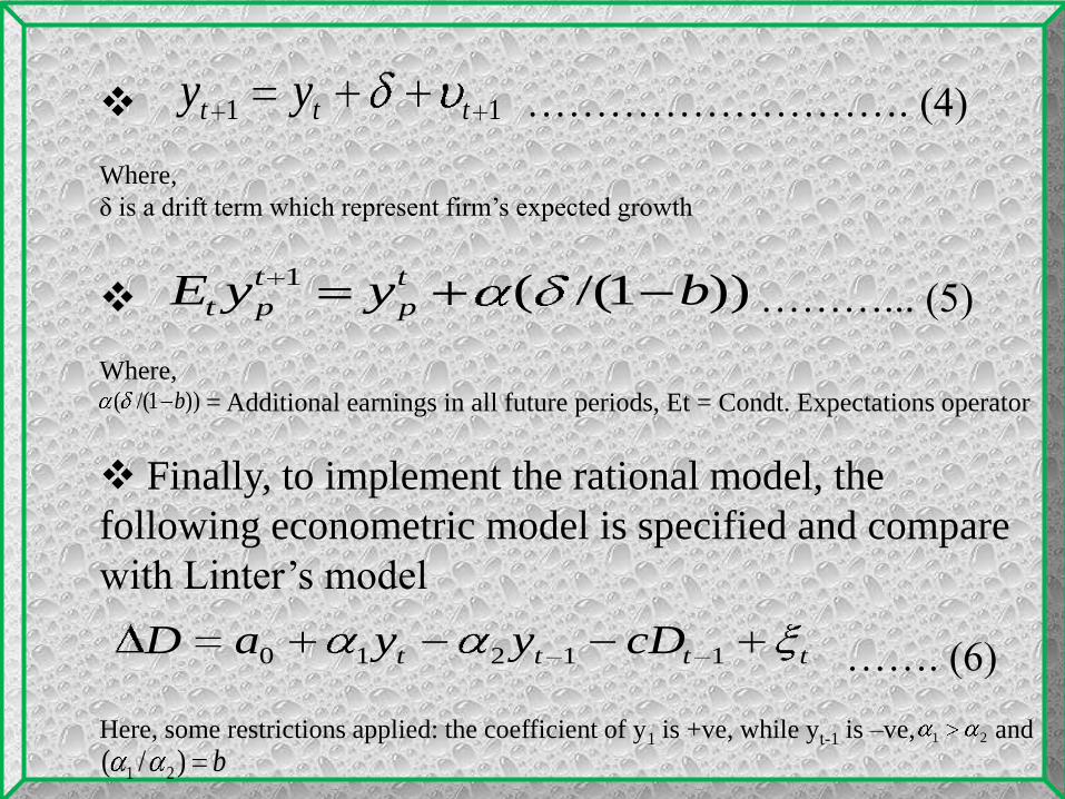
………………………. (4)

Where,

δ is a drift term which represent firm’s expected growth

………... (5)

Where,

= Additional earnings in all future periods, Et = Condt. Expectations operator

Finally, to implement the rational model, the

following econometric model is specified and compare

with Linter’s model

……. (6)

Here, some restrictions applied: the coefficient of y1 is +ve, while yt-1 is –ve, and

11 ttt yy

))1/((1 byyE t

p

t

pt

))1/(( b

tttt cDyyaD 11210

21

b)/( 21

Table 1 – Estimated coefficients for the Rational and Lintner

model for U.S. and Japanese firms in selected industriesRational

Model & t

Rational Model & t

+ - - - + - - -

Against the priori

sign

Findings:For both countries, the coefficients have as per the priori sign so that .21

For both models the constant terms numerically larger and statistically more significant for Japanese firms than for U.S. firms.

Against the priori

sign

The results support the Lintner’sarguments that constant term is non-negative that indicates gradual growth in dividend payments.

21 αα

Table 2- Predictive

comparisons of the

Rational and

Lintner models

The in-sample as

well as the out-of-

sample values for

R2 are higher for

the Rational model

than for the Lintner

model for 11 out of

12 industry groups

for both the U.S.

and Japan.

With this, the study

The major

conclusion is

Rational model

yields somewhat

better predictions

of the dividend

payouts of firms

Exception Exception

Table 3 – Predictive power tests of pooling and endogeneity

More specifically, under the pooling heading

there is clear evidence that Rational model

outperform whereas under the endogeneity

heading except 4 out of 11 industry groups, a

similar results emerges from the out-of-

sample subgroup.

The finding of the R2 comparison under the

Pooling and Endogeneity heading indicated

that Rational model outperforms the Lintner

model for both subgroups of the firms.

The study concluded that under the rational

expectations hypothesis for a firm’s management, an

econometric specification of the firm’s dividend

behavior results the inclusion of a lagged earnings

variable in the Lintner model and,

The study provided empirically testable sign and

magnitude restrictions on the estimated coefficients of

the resulting model of dividend behavior.

What concludes from the whole analysis?

StrengthThe detailed description of the methodology and procedures

Discussion of the basic assumptions of the OLS regression

model, and

Specified the additional explanatory variable in Lintner model,

and

Contribution to the literature

WeaknessConclusions are based only on the R2 comparison criteria.

(By adding one extra variable in the existing Lintner model, it

gives higher R2 because the addition of new explanatory variable

in the regression model always produce the higher coefficient of

determination!)

Critical appreciation of the study

Thank you.