Abstract

Bureau International des Poids et Mesures

Rapport BIPM -89/1

Shape Measurements of Standard Length Scales

Using Interferometry with Small Angles of Incidence

by Lennart Robertsson

An interferometric technique for surface shape measurements on standard line scales has

been developed and tested. By using small angles of incidence for the laser light to the surface

a variable sensitivity, practical dimensions on the interferograms and insensitivity to surface

roughness can be obtained. Measurements on a 300 mm line scale are included as a demon­

stration. With the optical components used an accuracy in the surface determination of about

2.5 ~m was obtained.

1 INTRODUCTION

The definition of length in tenns of propagation of electromagnetic waves allows for very

accurate length standards, limited in principle only by the accuracy to which the frequency of

the particular light sources are known at the time. More and more accurate frequency

measurements and better laser systems will yield better and better standards without having to

change the definition of the metre. The present best frequency determinations are around 10-10

in relative uncertainty (3 cr) [1],[2].

For the practical realization of the metre interferometric techniques are nonnally used and

standard lengths are transferred in the form of line scales and end gauges, as can be expected,

with a lower precision.

To determine to what precision the calibration of line scales can be done a large inter­

national comparison of length scale measurements has been organized and reported recently by

the BIPM [3]. It was concluded in this comparison that the reproducibility of length

measurements was not as good as one could expect from individual instrumental perfonnance.

The standard deviation of one laboratory with respect to the mean of the measurements of the

length of a 1 m ruled material standard was found to be of the order of 10-7, in contrast to the

corresponding estimated uncertainties given for the individual laboratories participating in the

comparison, which were, in average, around 3.10-8• Hence, systematic errors exist which have

been underestimated when calculating the uncertainties in the experimental data.

Indications of a correlation between shape and'length was mentioned in reference [3]. The

vertical deviation from a plane of the scale, given in one ofthe measurements [4], and deviations

in the relative calibration for each decimetre line are both shown in Fig. 1. Relative calibration

refers to the values of the deviations for each decimetre line from that of an ideal scale of 1 m

and perfectly divided in 1000 mm lines. It can indeed be seen from the similarity of the structures

of the curves that a correlation between these two quantities seems to exist. It can however not

be concluded whether this correlation is due to the fact that the measured values directly are

affected by the shape of the scale or if the lines actually are displaced. Such a correlated dis­

placement could have occurred in the generation process of the lines if the technique to engrave

the lines also was dependent on the scale shape.

It is anyhow of interest to be able to monitor the surface shape of standard length scales

to detect geometrical instabilities and gain control over factors causing such.

- 2-

We present below an interferometric technique for the characterization of line scale

surfaces, for long as well as for short scales. Similar techniques applied to different surfaces

have been described earlier [5]. By using a projection of the surface to be measured, instead of

the usual normal incidence of the laser light, several advantages can be obtained. This is described

in the following section.

Measurements on a 300 mm scale are included as a demonstration of the performance of this

technique.

2 MEASURING PRINCIPLE

The surface function, z (x , y), of a scale, here defined as the deviation from an average

plane trough the surface, is from experience [3] expected to be in the range of some 10-50 ~m.

Such measured deviations for the surface are the sum of two effects, the actual "straightness"

and superimposed on it variations in thickness of the scale.

This interval is in a practical working range for good mechanical probes. Unfortunately,

such probes work with mechanical contact to the surface that is being measured. This is not to

be recommended when measuring the front side of the scale since a metallic contact probe could

give surface damages, and in worst case deform some engraved lines and thereby ruin the whole

scale. It could however be used to measure the three remaining sides.

A second drawback with mechanical probes is the unavoidable pressure exerted by the probe

on the surface which, in principle, deforms the scale. This effect can however be estimated and

adjusted so as to minimize the introduced errors.

Alternatively, interferometric methods for surface measurements are known to be very

useful tools, giving immediate and contactless surface contour information with a very high

sensitivity. Unfortunately, the working range of interest here is at the upper limit of what is

practical for an interferometric technique and is therefore not optimal. Furthermore, and much

more serious, are the large dimensions of the surfaces to be covered making a straight forward

interferometric measurement practically impossible.

Realizing the advantage of interferometric techniques we have made a small variation of

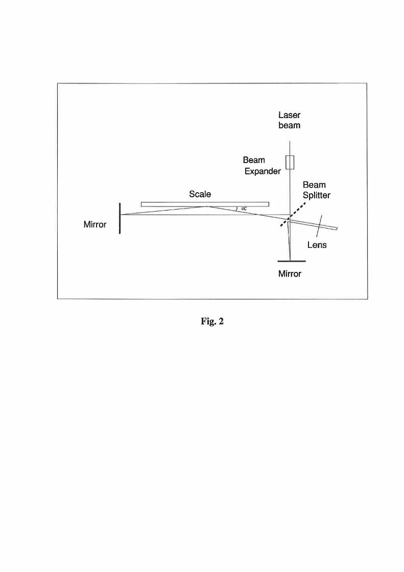
a Michelson interferometer so as to overcome the difficulties just mentioned. The schematics

of the set up used here is shown in Fig. 2. One sees here a traditional Michelson interferometer

but with an angle off-set for the returning beams in the interferometer. For the long arm of the

interferometer the beam is reflected in the surface to be studied. The projection of the surface

has to be covered by the aperture of the interferometer if an interferogram of the whole surface

- 3 -

is to be obtained.

The most important feature of this set up is that the laser beam, incident at a low angle to the

surface, sees a projection of the surface and its irregularities. This gives the following advantages:

*

*

*

practical dimensions of the projections of the surface and the interferogram.

a reduced sensitivity to surface roughness which, makes possible measurements

even on rough "non-mirror" surfaces i.e. all sides of the scale can be measured.

Light under glancing incidence will experience a much reduced surface

micro-roughness and hence a much less scatter will occur.

a reduced and variable sensitivity adaptable to the deviation expected. The

sensitivity is scaled as sine of the angle, a, used, c.f. Fig. 2. This is of limited

importance since with lower sensitivity a shorter projection is obtained in the

recording media, giving a reduced number of fringes on a smaller surface, so as

the fringe density in the interference pattern is kept constant.

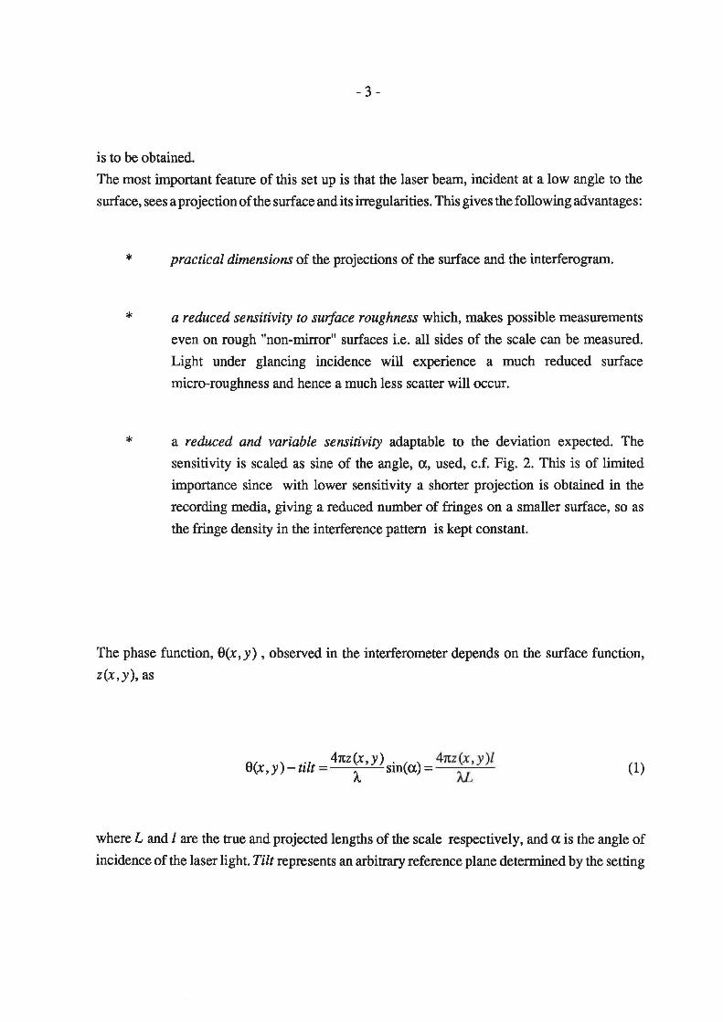
The phase function, S(x, y) , observed in the interferometer depends on the surface function,

z(x,y), as

S( ) '1 _ 41tz(x,y) . ( ) _ 41tz(x ,y )1 x,y -tl t- A. sm a - 'AL (1)

where L and I are the true and projected lengths of the scale respectively, and a is the angle of

incidence of the laser light. Tilt represents an arbitrary reference plane determined by the setting

-4-

of the reference mirror. This effect is only indicated in eq. 1 and not later equations since it is

eliminated in the data evaluation step by the fitting and subtraction of a plane to the surface

function.

For incidence at right angles this gives a fringe distance of 'Ai2 as expected. For an angle of

incidence a we get the fringe distance 'Ai(2sin(a». This can be expressed as an effective

wavelength

2.1 Error estimation

A. A.cJf = ~( ) = ALII sm a

(2).

For the use in section 3.3 we already here derive some relations for the estimation of

uncertainties in the determination of the surface function. Using eq. 1, one can, given the

phase function, determine the surface function. To be able to estimate the accuracy in this

determination let us differentiate eq. 1:

(3).

de is then the phase resolution in the evaluation of the interferograms. More difficult is to

determine the error in the effective wavelength, dA.cJf. In eq. 2 one can see that a direct

measurement of a or a determination of the projected length gives the effective wavelength.

Here we have deduced the projected length from the interferogram using the aperture of the

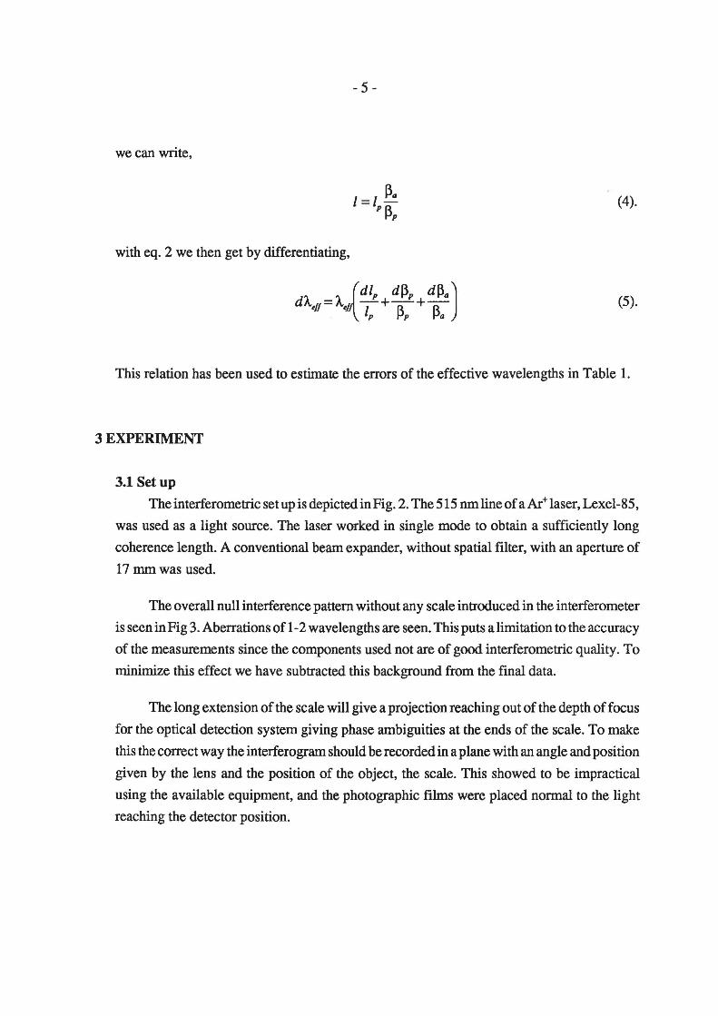
interferometer as a reference length. Using the following notations,

~p - interferometer aperture on

photograph

~a - true interferometer aperture

lp - projected length on photo

- 5 -

we can write,

(4).

with eq. 2 we then get by differentiating,

(5).

This relation has been used to estimate the errors of the effective wavelengths in Table 1.

3 EXPERIMENT

3.1 Set up

The interferometric setupis depicted in Fig. 2. TheSIS nmlineofaAr+laser, Lexel-85,

was used as a light source. The laser worked in single mode to obtain a sufficiently long

coherence length. A conventional beam expander, without spatial filter, with an aperture of

17 mm was used.

The overall null interference pattern without any scale introduced in the interferometer

is seen in Fig 3. Aberrations of 1-2 wavelengths are seen. This puts a limitation to the accuracy

of the measurements since the components used not are of good interferometric quality. To

minimize this effect we have subtracted this background from the final data.

The long extension of the scale will give a projection reaching out of the depth of focus

for the optical detection system giving phase ambiguities at the ends of the scale. To make

this the correct way the interferogram should be recorded in a plane with an angle and position

given by the lens and the position of the object, the scale. This showed to be impractical

using the available equipment, and the photographic films were placed normal to the light

reaching the detector position.

- 6-

3.2 Measurements

As a test of the measuring principle and set up, measurements on a 300 mm H-bar

scale have been perfonned.

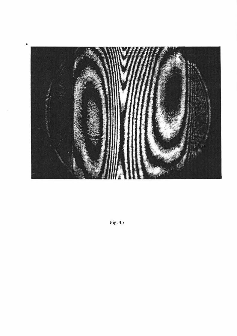
In Figs. 4 a-c. interferograms are shown recorded on photographic films positioned in the

plane of projection in the detection arm for a point on the middle of the scale. The most

smooth and nice interference pattern was, as expected, obtained from the front surface of

the scale, 4a. In figures 4b and 4c one can see that also the sides of the scale give with this

technique interference patterns of good qUality. An attempt to obtain interference fringes at

nonnal incidence to the side surfaces gave no usable results.

The ambiguity in the sign of the phase variations were resolved by observing the movements

in the interference pattern when slightly moving the reference mirror.

3.3 Evaluation and results

As was mentioned above the aperture of the interferometer is 17 mm, set by the beam

expander. This diameter of the circular reference beam serve as a reference distance on the

recorded interferograms , which can be used to determine the projected length of the scale,

c.f. Fig. 4c. With the projected length and the true length (here 300 mm) known, the angle

of incidence and the effective wavelength can be calculated using eq. 2. These values are

collected in Table 1. For the recordings made here the effective wavelength were about 12

Jlm corresponding to a angle of incidence of some 2 deg.

The estimated uncertainties in the effective wavelength, using eq. 5, and the value d~a=O.1

mm, are included in the parentheses in the fifth column in Table 1.

Phase maps ofthe interference area were evaluated in a 11x11 matrix giving 121 data

points. Since the phase function is evaluated in discrete points a numerical low pass filter

step has been applied to filter out surface function frequencies contained under the Nyquist

frequency. If the surface function does contain higher frequencies these will be lost in this

step and a certain alaising will occur.

For the purpose of demonstration we assume rapid changes in the surface function to be

small and we will make no further considerations about such effects here in this report.

The corresponding surface functions obtained using equation 1, the effective wave­

length and the phase maps are shown in Figs. 5a-c.

-7-

In Fig. 6a-c are shown profiles of the surface functions taken at the middle of the scale in

the length direction. For these diagrams also the curved null surface, given in the interfer­

ometer, has been subtracted, giving more accurate data. One can see that the deviations are

of the order of some tens of micrometers, as expected.

The phase determination in the evaluation of the phase function can be made with an

absolute error of de = 27t15 which then at each point give an maximum error of about 1 ~m

using eq. 3. This is an effect of the limitations in manual evaluation. Electronic techniques

would here improve the accuracy with at least a factor of ten.

Furthermore, the uncertainties in the effective wavelengths, around 0.3 ~m, give for

large values of e = 207t, a maximum error of about 1.5 ~m Thus the total maximum uncer­

tainty, according to eq. 3, for the determination of the surface function is 2.5 ~m.

4 CONCLUSION

It has been demonstrated that the technique using a projection of the studied surface indeed

is a good way to determine the shape of standard scales. With the technique described here a

measurement of the shape of the different sides of the scale can be made in some few minutes,

provided a fixed set up and computerized data evaluation. The uncertainty in this measurement

is limited by the manual evaluation of the interferogram and the determination of the effective

wavelength to around 2.5 ~m.

Shape measurements ought to be done on a regular basis; possibly every time the scale is

calibrated to be able to make more firm conclusions in the case of unexpected values of the

measured length. In principle this type of measurements could be done simultaneously with the

length measurements (in our case inside the comparator chamber) to defmitely determine the

shape in the position and environment where the accurate length measurement is made. For

instance, effects like "bad holders" ,position instability, and alike could in this way be identified,

at the same time as the surface function is determined and compared to earlier measurement to

see if any geometrical change has occurred, possibly caused by improper handling routines.

Several improvements of the set up described above can be made. Both the quality of the

optics and size of the aperture in the interferometer should be improved. This would increase

the working range and the accuracy. To further improve the dynamic range and to definitely

resolve the phase ambiguities, a phase shifting technique would be well suited. Phase shifting

- 8 -

interferometry for surface covering interferometers involve a large number of data processing

and it is therefore almost necessary to use a computer. Digitalization of the interference pattern

and transfer to a computer then gives better performance, result storage and presentation.

September 1989

- 9 -

REFERENCES

[1] "Documents Concerning the New Definition of the Meter", Metrolo~ia. 19, 1984,

pp. 163-177.

[2] "The Continuity of the Meter: The Redefinition of the Meter and the Speed Of

Visible Light", 1. of Res. of the National Bureau of Standards. 92, 1987, p. 11.

[3] RAMON J., GIACOMO P. and CARRE P., International Comparison of

Measurements of Line Scales 1976-1984, Metrolo~a. 24, 1987, pp. 187-194.

[4] see reference [3], table 6a, data N° 12.

[5] ARCHBOLD E., BURCH J.M. and ENNOS A.E.,

I. Scir InstIum .. 44, 1967, pp. 489-494.

- 10-

Table 1 Evaluation of effective wavelength for the three recordings 4a, 4b and 4c.

Diameter

photo

[mm]

125(1)

142(1)

130(1)

Length

photo

[mm]

100(1)

100(1)

94(1)

Projected

length

I

[mm]

13.6

12.0

12.3

Angle of

incidence

[deg]

2.60

2.29

2.35

Effective

wavelength

11.34(27)

12.88(30)

12.55(30)

- 11 -

FIGURE CAPTIONS

Fig. 1.

Fig. 2.

Fig. 3.

Fig.4a

Fig.4b

Fig.4c

Fig.5a

Fig.5b

Fig.5c

Fig.6a

Fig.6b

Fig.6c

The dotted curve shows the deviation in height from a line crossing the two end

points of the surface.

The solid curve gives the relative calibration (see text) forthe ten decimetre lines.

The interferometric set up.

Null surface measured in the interferometer. A curved background is seen as a

result of limitations in the optical components used.

Photographic recording of the interference pattern of the front side of the scale.

Photographic recording of the interference pattern of one side of the scale.

Photographic recording of the interference pattern of the other side of the scale.

Surface function corresponding to the interferogram in Fig. 4a.

Surface function corresponding to the interferogram in Fig. 4b.

Surface function corresponding to the interferogram in Fig. 4c.

Profile of the surface function taken at the middle of the scale in the length

direction. Front side.

Profile of the surface function taken at the middle of the scale in the length

direction. Side.

Profile of the surface function taken at the middle of the scale in the length

direction. Side.

1,000 r----------------------------..., 100

800 80

"A ......... "',; .........

'" .... " If'" \\ "A / ,/ \

I \ " \ I ,,, \

/ '.'tf" \ I \

I \ I \

//"~ \ , \

600

400

200

60

40

20 \

" , '" " o~--~~--~--~--~----~--~----~--~----~--~~o o 2 3 4 5 6 7 8 9 10

Decimetre line

Fig. 1

length

• height

---tr--

Laser beam

Beam [ Expander ~

Beam Scale Splitter

~

~ #

# #

I Mirror ~ i:--#

I~

Lens

Mirror

Fig. 2

1,000 ._---------------------------. 100 length

• height

800 80 ---0---

600 60

40

200 20

o~--~~--~-~-~~-~-~--~-~--~-__ ~o o 2 3 4 5 6 7 8 9 10

Decimetre line

Fig. 1

Laser beam

,

Beam [ Expander 0

Beam Scale Splitter

• #

~ # #

~ ~ J Mirror #

I -..J

Lens

Mirror

Fig. 2

•

Fig. 3

•

Fig.4b

Fig.4a

•

Fig.4c

Fig. Sa

Fig.5b

Fig. Se

Height [JAm]

~r--------------------------------------------------,

40

30

20

10

o~----~--~----~--~--~----~--~--~----~--__ ~ o 1 2 3 4 5 6 7 8 9 10

Decimetre line

Fig.6a

Height [pm]

10r-------------------------------------------------,

o

(10)

(20)

(30)

(~)~~--~--~----~--~--~----~--~--~----~--~~ o 1 2 3 4 5 6 7 8 9 10

Decimetre line

Fig.6b

Height [pm]

~r-----------------------------------------------------~

40

30

20

10

o~~--~----~--~----~--~----~--~----~--~----~~ o 1 2 3 4 5 6 7 8 9 10

Decimetre line

Fig.6c