rapid monitoring and assessment of drought in papua new
TRANSCRIPT

Rapid Monitoring and Assessment of Drought in Papua New Guinea using
Satellite Imagery
Final Report
to
United Nations Development Program
Port Moresby
Papua New Guinea
by
Phil N. Bierwirth1 and Tim R. McVicar
2
September 1998
1 Australian Geological Survey Organisation, PO Box 378, Canberra 2601, Australia.
2 CSIRO Land and Water, PO Box 1666, Canberra 2601, Australia.

D:\PNG\PNG_DGHT.DOC 2/11/2013 ii
© 1998 Australian Geological Survey Organisation and CSIRO Australia, All Rights
Reserved
This work is copyright. It may be reproduced in whole or in part for study, research or
educational training purposes subject to the inclusion of an acknowledgment of the source.
Reproduction for commercial usage (including commercial training courses) or sale purposes
requires written permission of Australian Geological Survey Organisation and CSIRO
Australia.
Authors
Phil N. Bierwirth1 and Tim R. McVicar
2
1 Australian Geological Survey Organisation, PO Box 378, Canberra 2601, Australia.
[email protected] 61-2-6249-9231
2 CSIRO Land and Water, PO Box 1666, Canberra 2601, Australia.
[email protected] 61-2-6246-5741
ISBN
For bibliographic purposes, this document may be cited as:
Bierwirth, P. N. and McVicar, T. R. (1998) Rapid Monitoring and Assessment of Drought in
Papua New Guinea using Satellite Imagery. Consultancy Report to United Nations
Development Program, Port Moresby, Papua New Guinea, pp. 60.
For additional copies of this publication please contact:
Publication Enquires
CANBERRA
ACT 2601
AUSTRALIA
enquiries@
http://www

D:\PNG\PNG_DGHT.DOC 2/11/2013 i
Executive Summary
Remotely sensed data from the Advanced Very High Resolution Radiometer (AVHRR)
sensor was used to rapidly monitor and assess the 1997 drought experienced in Papua New
Guinea (PNG). Data was purchased for a normal year (1996), the drought (1997) and for the
year of recovery (1998). To overcome the problem of high amounts of cloud coverage
experienced in the tropics, 4-week and 8-week composite data were used. The processing
pathway developed in this project, which has been transferred to local scientists, is fully
documented in this report. The Normalised Difference Vegetation Index (NDVI) and surface
temperature (Ts) were both used. To utilise the negative correlation exhibited between these
two variables the ratio of Ts/NDVI was plotted as a time series and mapped as time
difference images. This provided a rapid indicator of drought, which does not require
ancillary meteorological data.

D:\PNG\PNG_DGHT.DOC 2/11/2013 ii
Institutional Acronyms
ACRES Australian Centre for REmote Sensing
AGSO Australian Geological Survey Organisation
CSIRO Commonwealth Scientific Industrial Research Organisation
DAL Department of Agriculture and Livestock (PNG)
NASA National Aeronautics and Space Administration (USA)
NOAA National Oceanographic and Atmospheric Administration (USA)
PNGGS Papua New Guinea Geological Survey
UNDP United Nations Development Program
Scientific Acronyms
AE Available Energy
AVHRR Advanced Very High Radiometric Resolution
BIL Band Interleaved by Line
BRDF Bidirectional Reflectance Distribution Function
CWSI Crop Water Stress Index
DEM Digital Elevation Model
EMS Electromagnetic Spectrum
ENSO El Nino Southern Oscillation
ERS Earth Resource Satellite
ET Evapotranspiration
GAC Global Area Coverage
GIS Geographic Information System
GMS Geostationary Meteorological Satellite
JERS Japanese Earth Resources Satellite
LAC Local Area Coverage
LAI Leaf Area Index
MODIS MODerate-resolution Imaging Spectroradiometer
MSS Multi-Spectral Sensor
NDTI Normalised Difference Temperature Index
NDVI Normalised Difference Vegetation Index
NIR Near InfraRed
RADAR RAdio Detection And Ranging
SAR Synthetic Aperture RADAR
SEB Surface Energy Balance
SOI Southern Oscillation Index
TM Thematic Mapper
Ts Surface Temperature
VISSR Visible and Infrared Spin Scan Radiometer
VITT Vegetation Index Temperature Trapezoid

D:\PNG\PNG_DGHT.DOC 2/11/2013 iii
1.0 INTRODUCTION ............................................................................................................................ 1
2.0 PAPUA NEW GUINEA AND THE 1997 DROUGHT .................................................................. 1
3.0 BACKGROUND OF REMOTE SENSING ................................................................................... 3
3.1 REFLECTIVE REMOTE SENSING ............................................................................................................ 5
3.2 THERMAL REMOTE SENSING ............................................................................................................... 7
3.3 MICROWAVE REMOTE SENSING ........................................................................................................... 9
4.0 METHODS ...................................................................................................................................... 12
4.1 SELECTION OF REMOTELY SENSED DATA TO ASSESS THE PNG DROUGHT ........................................ 12
4.2 ESTABLISHING THE AVHRR TIME SERIES ......................................................................................... 12
4.3 DESCRIPTION OF THE AVHRR TIME SERIES. ..................................................................................... 15
5.0 TECHNICAL PROCEDURES FOR IMPLEMENTING PNG_DATS ..................................... 19
5.1 DATA LOCATIONS .............................................................................................................................. 19
5.2 RECEIVING NOAA AVHRR DATA FROM TASMANIA ......................................................................... 19
5.3 IMPORTING INTO ER-MAPPER AND USING FORMULAS TO EXTRACT INFORMATION ............................. 20
5.4 CREATING AN NDVI ALGORITHM FROM NOAA/AVHRR 4 WEEK COMPOSITE IMAGES ..................... 22
5.5 USING THE AGSO/CSIRO ER-MAPPER ALGORITHM SYSTEM DEVELOPED AT THE PNGGS .............. 24
5.5.1 Creating a data-set for new AVHRR data ................................................................................. 25
5.5.2 Adding to and creating 4 week composite display and printing algorithms. ............................. 27
5.5.3 Adding to and creating 4- week difference image display and printing algorithms. ................. 28
5.5.4. Adding to and creating 8-week composite display and printing algorithms. ........................... 29
5.5.5 Adding to and creating 8-week difference image display and printing algorithms. ................. 29
5.6 MAKING A POSTER ALGORITHM ......................................................................................................... 31
6.0 ANALYSIS OF THE REMOTELY SENSED IMAGERY ......................................................... 34
6.1 INITIAL ANALYSIS AND VISUALIZATION OF PNG_DATS ................................................................... 34
6.2 EXPLORING THE DATA AT THE PROVINCE LEVEL ............................................................................... 38
6.3 COMBINING THE DATA WITH METEOROLOGICAL DATA SETS ............................................................... 44
7.0 RECOMMENDATIONS: OPPORTUNITIES & IMPROVEMENTS ...................................... 46
7.1 OPPORTUNITIES ................................................................................................................................. 46
7.2 RECOMMENDED FUTURE IMPROVEMENTS ......................................................................................... 47
8.0 CONCLUSIONS ............................................................................................................................. 48
9.0 ACKNOWLEDGMENTS .............................................................................................................. 48
10.0 REFERENCES ............................................................................................................................. 49
11.0 APPENDIX 1 ORGANISATIONS AND INDIVIDUALS CONSULTED. .............................. 54
12.0 APPENDIX 2: LISTING OF LOOK-UP-TABLES (LUT) ....................................................... 55

D:\PNG\PNG_DGHT.DOC 2/11/2013 1
1.0 Introduction
This report demonstrates how hi-frequency remote sensing has been used to monitor and
assess the 1997 drought in Papua New Guinea (PNG). This project was funded by the United
Nations Development Program (UNDP). The funds allowed for suitable satellite imagery to
be acquired, and for a short visit (2 weeks) by the two authors of this report to PNG. This
report documents the establishment of the remote sensing data base, the technology transfer
and the data analysis that was undertaken during the course of this project.
The stated aims of this project are to:
1. determine if hi-frequency remotely sensed data allows drought conditions in PNG to be
monitored;
2. transfer the technology, if monitoring of drought is possible, so that Officials from several
PNG National Government Departments have the ability to undertake the analysis of hi-
frequency remote sensing data;
3. provide assistance with the scientific interpretation of the remotely sensed data of the
drought experienced by PNG in 1997; and
4. provide recommendations, based on the findings of 2 and 3 above, on operational systems
that could be established, using readily available data to assist PNG in monitoring and
assessing the 1997 drought. Consideration is given to developing an early warning of
future drought situations. The monitoring of actual, rather than potential conditions, is still
considered important.
In undertaking this project visits were made to organisations that had first hand experience in
dealing with the assessment and response to the 1997 drought. These included the:
• Papua New Guinea Geological Survey (PNGGS)
• Papua New Guinea Department of Agriculture and Livestock (DAL)
• Papua New Guinea Meteorological Office
• Australian National University, Department of Human Geography
• Australian National University, Centre for Resources and Environmental Studies
For a comprehensive listing of individuals contacted during this project, refer to Appendix 1.
An introduction to PNG and the drought of 1997 is given in the following section. A
background to remote sensing is provided in Section 3. Specialists in any of these areas need
not wade through this material; they provide full context.
2.0 Papua New Guinea and the 1997 Drought
Papua New Guinea is comprised of the eastern half of the island of New Guinea and the
archipelago extending to the East of the main island. The western portion of the island of
New Guinea is Irian Jaya, Indonesia. PNG extends from the equator to 12 degrees South and
longitudes 141 to 156 degrees East. The total land area is over 460,000 km2. The main island
of PNG is 1,100 km east-west and 900 km north-south, see Fig. 1.

D:\PNG\PNG_DGHT.DOC 2/11/2013 2
Drought is a complex natural event. A universally accepted definition of drought does not
exist (Wilhite, 1993). It is acknowledged that the major cause of drought is lower than
average rainfall. The rainfall deficit will have different impacts depending on other factors
including, meteorological conditions, ecosystem type, and social and economic
circumstances. Currently, there are four major types of drought which are broadly defined and
agreed upon in the scientific literature (WMO, 1975, Wilhite and Glantz, 1985, White, 1990,
Alley, 1984, Alley, 1985). These are:
1. meteorological drought, which is generally regarded as being lower than average
precipitation for some time period. In some cases air temperature and precipitation
anomalies may be combined;
2. agricultural drought, occurs when plant available water, from precipitation and water
stored in the soil, falls below that required by a plant community during a critical growth
stage. This leads to below average yields in both pastoral and crop producing regions;
3. hydrologic drought is generally defined by one or a combination of factors such as stream
flow, reservoir storage and groundwater; and
4. socioeconomic drought is defined in terms of loss from an average or expected return. It
can be measured by both social and economic indicators, of which profit is only one.
We consider drought to be a period when lower than average rainfall was received and
agricultural production systems fell below capacity. This definition is a hybrid between the
classic meteorological and agricultural drought definitions. In this study we are looking for
broad indicators of drought from hi-frequency remotely sensed data; we are not attempting to
use this data to define and map drought conditions for legislative measures.
Drought conditions in PNG may be defined as occurring when rainfall was lower than
average for periods greater than 10 weeks (Bourke pers. comm.). There is a long and well
documented history of drought events occurring in PNG, often associated with El Nino events
(Nicholls, 1973, Allen, 1989, Allen et al., 1989). In PNG drought conditions affect the food
supply to the subsistence based agricultural communities in two ways: (I) decrease of plant
available water; and (II) frost occurrence in the highlands. The lack of rainfall decreases the
plant available water, which in turn may result in reduction of plant cover. This affects the
production of food relied upon by the subsistence agricultural communities. This reduction in
plant cover is one parameter that is observed using remotely sensed data, see section 3.1.
During dry conditions more incoming short-wave radiation reaches the ground (due to there
being less cloud cover) and more of this is partitioned into the sensible heat flux (rather than
the latent heat flux), resulting in higher land surface temperatures, see section 3.2. The
response of land surface temperatures (an increase) is slight faster than the response of plant
cover (a decrease) due to reduced moisture availability associated with drought conditions.
Within the PNG highlands there is a belt of dense human habitation between the altitudes of 1
400m to 2 850m above sea level (Brookfield and Allen, 1989). Drought conditions are
associated with low amounts of cloud cover. Due to the cloudless nights and the consequent
loss of long-wave radiation, surface cooling results in frosts. The highland agricultural
systems are subsistence-based; relying heavily on the frost intolerant sweet potato. If frost is
experienced prior to tuber bulking the crop may be delayed by several months, however, if
frost occurs during or after the bulking phase the subsequent tubers are inedible (Bourke,
1989). Recently some frost tolerant crops have been introduced.

D:\PNG\PNG_DGHT.DOC 2/11/2013 3
During the 1997 drought, low plant water availability and frosts were experienced (Bourke,
1998, Allen et al., 1997, Allen and Bourke, 1997, Allen, 1998). This meant that populations
relying on subsistence-based agriculture needed supplementary food supplies. Some 1.2
million rural villagers suffered a severe, and in some cases fatal, food shortage during the
1997 drought event in PNG. This is almost 40 percent of the rural population (Allen and
Bourke, 1997, Allen, 1998). The 1997 event is considered to the the “drought of the century”
(Bourke, 1998), the associated food and water shortages strained emergency services beyond
their limits (Bourke, 1998, Allen, 1998). The onset of drought can cause both immediate food
shortages (due to frosts) and longer term food shortages (due to decreased plant water
availability). Both the onset of drought conditions and the recovery from drought are
important factors in a drought event; both phases are considered in this report.
The percent divergence from monthly average rainfall, shown in Fig. 2, reveals that many
stations during 1997 received below average rainfall for several months. Large areas of PNG
have no reliable meteorological ground recording facilities (Fig. 2). Some of these areas are
sparsely populated. However, the number of ground based stations has been decreasing over
the last 20 years. A characteristic of remote sensing is its synoptic coverage which provides
vast opportunities for monitoring the 1997 drought event in PNG.
3.0 Background of Remote Sensing
Remote sensing is the acquisition of digital data in the gamma, reflective, thermal or
microwave portions of the electromagnetic spectrum (EMS). Fig. 3 is a schematic diagram of
electromagnetic radiation. Measurements of the EMS are be made either from satellite,
aircraft or ground-based systems, but it is characteristically at a distance (or “remote”) from
the target. Due to the large spatial extent of PNG, this paper will focus on data gathered from
satellite remote sensing systems.
Remotely sensed images are recorded digitally by sensors on board the satellites. A schematic
of satellite based remote sensing is shown in Fig. 4. The resulting images can be manipulated
by computers to highlight features of soils, vegetation and clouds. Each pixel, or picture
element, contributing to the image is a measurement of a particular wavelength of
electromagnetic radiation at a particular spatial scale for a particular location at a specific
time. The most common display of remotely sensed data is a single overpass, which non-
remote sensing specialists may think of as a ‘satellite photo’.
Electric field
Magnetic field
Directionof travel
E
H
λ

D:\PNG\PNG_DGHT.DOC 2/11/2013 4
Fig. 3: An electromagnetic wave comprises two sinusoidal waves: an electric and a magnetic
wave. Wavelength (λ ) is the distance between successive wave peaks. Adapted from
(Harrison and Jupp, 1989).
Remotely sensed data are spatially dense. This means that for the extent of the image it is a
census at a particular spatial scale and electromagnetic wavelength. It is not a point sample.
There may be distances of 200 kilometers between meteorological stations, or field sites.
Remotely sensed data are measurements at, say, 1 km spatial resolution for each and every
one of the 200 km separating the stations.
Pixel depth 1.1 km
NOAASatellite
Spacecraft path direction
Swath width 2 700 km
θ
Earth su
rface
Pixel width5.5 km
Pixel width1.1 km
Altitude ~700 km
Fig. 4: Schematic of satellite operation. The data acquisition of the Advanced Very High
Resolution Radiometer (AVHRR) sensor operates onboard the United State Federal Agency
National Oceanographic and Atmospheric Administration (NOAA) series of satellites.
Adapted from (Harrison and Jupp, 1989).
When dealing with remotely sensed images, the extent, resolution (or integration) and density
of the spectral, spatial and temporal characteristics need to be kept in mind. Information for
current reflective and thermal satellite remote sensing systems is presented in Table 1 and for
current RADAR satellite based systems in Table 2.
Spectral:
• Spectral extent describes what portion of the electromagnetic spectrum is being sampled,
for example, is it just visible or does the range extend into the thermal.
• Spectral resolution refers to the bandwidths of each channel.
• Spectral density indicates the number of band in a particular portion of the EMS, for
example hyperspectral sensors have higher spectral density than broadband instruments.
D:\PNG\PNG_DGHT.DOC 2/11/2013 5
Spatial:
• Spatial extent is the area covered by the image.
• Spatial resolution refers to the smallest pixel or picture element acquired.
• Spatial density is complete, compare this with the spatial density of rainfall stations in the
example above.
Temporal:
• Temporal extent is the recording period over which the data is available, for some systems
data has been recorded for 25 years.
• Temporal resolution is the time that the data is acquired over, usually this is a matter of
seconds, compare this to the daily rainfall totals.
• Temporal density is the repeat characteristics of the satellite and for some applications the
availability of cloud free data.
The extent, resolution and density of remotely sensed data and other data sources, such as
ground based meteorological data, needs to be understood to be used in drought mapping and
monitoring systems.
Remote sensing of the land surface occurs at wavelengths of the EMS where the light can
pass through the Earth’s atmosphere with no, or little, interaction with the atmosphere. These
bands of the EMS are called ‘atmospheric windows’ and refer to the spectral extent in which
radiation reaching remote sensing instruments carries information about the Earth’s surface
conditions. These ‘atmospheric windows’ are defined by the transmittance of the constituents
of the Earth’s atmosphere. There are some gases which absorb all electromagnetic radiation in
certain wavelengths preventing these areas of the EMS being used for remote sensing. The
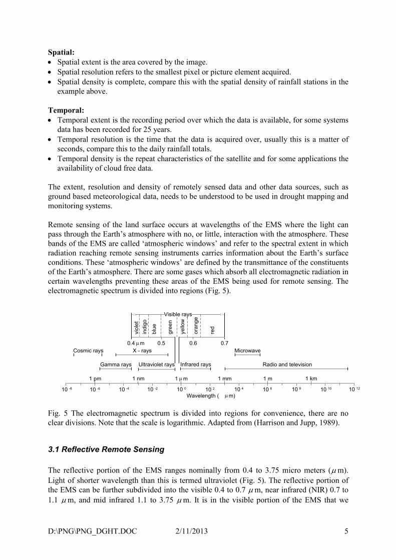
electromagnetic spectrum is divided into regions (Fig. 5).
Visible rays
violet
indigo
blue
green
yellow
orange
red
Cosmic rays X - rays Microwave
Gamma rays Ultraviolet rays Infrared rays Radio and television
1 pm 1 nm 1 µm 1 mm 1 m 1 km
10 -8 10 -6 10 -4 10 -2 10 0 10 2 10 4 10 6 10 8 10 10 10 12
0.70.60.50.4 µm
Wavelength ( µm)
Fig. 5 The electromagnetic spectrum is divided into regions for convenience, there are no
clear divisions. Note that the scale is logarithmic. Adapted from (Harrison and Jupp, 1989).
3.1 Reflective Remote Sensing
The reflective portion of the EMS ranges nominally from 0.4 to 3.75 micro meters (µm).
Light of shorter wavelength than this is termed ultraviolet (Fig. 5). The reflective portion of
the EMS can be further subdivided into the visible 0.4 to 0.7 µm, near infrared (NIR) 0.7 to
1.1 µm, and mid infrared 1.1 to 3.75 µm. It is in the visible portion of the EMS that we

D:\PNG\PNG_DGHT.DOC 2/11/2013 6
sense with our remote sensing device (eyes) which allow us to see. Different surface
reflective properties allow us to distinguish colour in the visible region of the EMS.
Chlorophyll pigments that are present in leaves absorb red light. In the NIR portion, radiation is
scattered by the internal spongy mesophyll leaf structure which leads to higher values in the NIR
channels. This interaction between leaves and the light that strikes them is one determinant of
the different responses in the red and NIR portions of reflective light (Fig. 6). Most vegetation
indices are combinations of these two reflective bands. The most common linear combinations
are the simple ratio (NIR/Red) and Normalised Difference Vegetation Index (NDVI) = (NIR-
Red)/(NIR+Red). Previous research has shown positive correlations exist between foliage
presence, including measurements of LAI (Tucker, 1979), and plant condition (Sellers, 1985),
and vegetation indices such as the simple ratio and NDVI. For a comprehensive listing of
vegetation indices refer to Tian (1989), Kaufman and Tanre (1992), Thenkabail et al. (1994)
and Leprieur et al. (1996).
Sun
Highly reflected infrared lig
ht
Reflecte
d green lig
ht
Green light
Blue light
Red light
Infrared light
Leafcellstructure
Remote sensor
Fig. 6: Schematic reflectance of a typical green leaf in cross section. The chloroplasts reflect the
green light absorb the red and blue wavelength for use on photosynthesis. The near infrared light
is highly scattered by water in the spongy mesophyll cells. Adapted from (Harrison and Jupp,
1989).

D:\PNG\PNG_DGHT.DOC 2/11/2013 7
While the amount of leaf is one determinant of the signal strength in the reflective portion of
the EMS there are several other important factors which control the acquired value. These
include the sun-target-sensor geometry. This will control the amount of shadow contributing
to the signal; the shadow may be driven by insolation effects due to regional topography and
may also be influenced by vegetation shadowing. This effect, termed the bidirectional
reflectance distribution function (BRDF) (Burgess and Pairman, 1997, Deering, 1989), is
characteristic of vegetation structure. Other effects in the reflective portion of the EMS
include changes in soil colour and changes in the observed signal due to changes in the
atmospheric component of the signal, including atmospheric precipitable water (Choudhury
and DiGirolamo, 1995, Hobbs, 1997), and changes in the response of the sensor over time.
The uses of the reflective portion of the EMS for drought assessment and monitoring are
reviewed by McVicar and Jupp (1998).
3.2 Thermal Remote Sensing
The thermal portion of the EMS ranges nominally from 3.75 to 12.5 micro meters (Fig. 5).
The radiant energy observed by sensors is emitted by the surface, be it land, ocean or cloud
top, and is a function of surface temperature. Models have been developed to allow surface
temperature to be extracted from thermal remote sensing. Prata (1994) and Prata et al. (1995)
review the algorithms and issues involved in the calculation of land surface temperatures.
Thermal remote sensing is an instantaneous observation of surface temperature which in turn
is related to the status of the surface energy balance (SEB). The SEB is driven by the net
radiation at the surface. During the daytime this is usually dominated by incoming short-wave
radiation from the sun, the amount reflected depending on the albedo of the surface. There are
also up and down welling long-wave components. At the ground surface the net allwave
radiation is balanced between the sensible, latent and ground heat fluxes. Over long periods
of time the ground heat flux averages out, and the SEB represents the balance with the
sensible and latent heat fluxes. During the day the measured surface temperature at the
Earth’s surface is, in part, dependent on the relative magnitude of the sensible and latent heat
fluxes.
The surface energy balance at any instant is given by:
where:
Rn is net all wavelength radiation (Wm-2);
E is the evapotranspiration (ET) flux (m sec-1) of water vapor;
λ is latent heat of vaporisation of water (J m-3);
H is sensible heat flux (W m-2), or the energy involved in the movement of the air and its
transfer to other objects (such as trees, grass etc); and
G is the ground heat flux into the soil or other storages (W m-2).
λE denotes the amount of energy needed to change a certain volume of water from liquid to
vapor, either by transpiration or evaporation. The combination of these two fluxes is called
nR = E+H+Gλ

D:\PNG\PNG_DGHT.DOC 2/11/2013 8
evapotranspiration. The net available energy (AE) at the Earth's surface, which is available for
conversion to other forms, can be written as AE R G E Hn= − = +λ
where the terms are defined as above. A key factor determining the observed surface
temperature is the partitioning of the AE into the latent and sensible heat fluxes. This is
governed by the amount of water available and the ease with which it is transferred from the
surface to the atmosphere, via ET. For given meteorological conditions there will also be a
potential ET which could occur if water was not limiting. The ratio of the actual to potential ET
is termed the moisture availability.
Thermal remotely sensed data can also be recorded at night. During the night, the SEB is
dominated by the release of heat from the ground, which was absorbed during the daylight
hours. The release of heat during the night is governed by how much was absorbed during the
day and the rate at which it is released after sunset. This is a function of the environment’s
capacity to store heat, which also depends on the amount of water stored in the environment.
The uses of the thermal portion of the EMS for drought assessment and monitoring are also
reviewed by McVicar and Jupp (1998).
Table 1. General description of current satellite sensors which acquire reflective and / or
thermal data which are useful for monitoring all of PNG for drought.
Satellite: Sensor Channel
#
Spectral
Resolution
Spatial
Resolution
(m) at nadir
Sample
Swath
Repeat
Cycle
Lifetime
GMS:VISSR1 1 500-750 nm 1250 hemisphere Hourly 1978 -
2 10.5-12.5 µm 5000 present
NOAA:AVHRR2 1 580-680 nm 1100 2700 km Every 1981 -
2 725-1100 nm " 12 present
3 3.55-3.93 µm " hours
4 10.5-11.3 µm "
5 11.5-12.5 µm "
LANDSAT:MSS3 4 500-600 nm 80 185 km Every 1972 -
5 600-700 nm " 16 present
6 700-800 nm " days
7 800-1100 nm "
LANDSAT:TM4 1 450-520 nm 30 185 km Every 1983 -
2 520-600 nm " 16 present
3 630-690 nm " days
4 769-900 nm "
5 1.55-1.75 µm "
7 2.08-2.35 µm "
6 10.4-12.5 µm 120

D:\PNG\PNG_DGHT.DOC 2/11/2013 9
1 GMS:VISSR is the Geostationary Meteorological Satellite (GMS) launched by Japan
provides images for Australasia. It is located above the equator at 1400E at an altitude of
some 36 000 km. The Visible and Infrared Spin Scan Radiometer (VISSR) is the main sensor
used for meteorological remote sensing. In other parts of the globe similar data are available
(Petty, 1995). The U.S. Geostationary Operational Satellite (GOES) series has a spatial
resolution at nadir similar to the VISSR. The European Meteosat, which carries the Meteosat
radiometer, has a spatial resolution at nadir of 2.5 km for the visible channel and 5 km for the
thermal IR. The Indian INSAT carries the VHRR radiometer which a spatial resolution at
nadir of 2.75 km for the visible channel and 11 km for the thermal IR.
2 NOAA:AVHRR refers to a series of satellites operated by the United State Federal Agency,
NOAA, National Oceanographic and Atmospheric Administration. The Advanced Very High
Resolution Radiometer (AVHRR) sensor operates on this platform. From 1978 to 1981 only
the first 4 channels were acquired. The NOAA series of satellites are polar orbiting at a height
of some 700 km, similar to the height of the LANDSAT series of satellites. AVHRR data are
acquired over a large swath width, compared to the LANDSAT data, due to the wide scan
angle, ± 55o, of the AVHRR sensor. The Local Area Coverage (LAC) pixel size is 1100 m at
the sub-satellite point, becoming 5400 m at the of edge of the swath. Global Area Coverage
(GAC) data are also recorded by the AVHRR sensor. GAC is a sub-sampling of the LAC data
and nominally has a 5 by 3 kilometer resolution. GAC data are recorded on board the satellite
and recorded at the NASA Goddard Space Flight Centre.
Soon AVHRR data will be superseded Moderate-Resolution Imaging Spectroradiometer
(MODIS) data. This is planned for launch in 1998 aboard EOS AM-1 and is the key
instrument in NASA’s Earth Observing System (EOS). A fleet of satellites is to be launched
over the next two decades. MODIS is anticipated to continue and enhance the high temporal
frequency coverage of remotely sensed data offered by the AVHRR sensor. MODIS has 36
bands with differing spatial resolutions (2 are 250m, 5 are 500m and the remaining 29 are 1
km) details of the increased spectral resolution of the bands can be found at the following
WWW address: http://modarch.gsfc.nasa.gov/MODIS/MODIS.html
3 LANDSAT:MSS refers to the multispectral sensor (MSS) on board the LANDSAT series of
satellites. From 1972 to 1983, for LANDSAT 1 - 3 the repeat cycle was 18 days. LANDSAT
is a polar orbiting sun synchronous satellite, which passes a given latitude at the same solar
time, it operates at a height of 700 km.
4 LANDSAT:TM refers to the thematic mapper (TM) sensor on board LANDSAT 4 and 5.
Channels and wavelengths are not ascending due to the late inclusion of channel 7.
3.3 Microwave Remote Sensing
The microwave portion of the EMS ranges nominally from 0.75 to 100 centimeters (Fig. 5).
Radio signals have wavelengths which are included in these bands. These systems can either
be active (the sensor sends its own signal) or passive (the background signal from the Earth’s
surface is observed). There are five smaller sections of this range which are used for remote
sensing. These are :
P band 100 - 30 cm;
L band 30 - 15 cm;

D:\PNG\PNG_DGHT.DOC 2/11/2013 10
S band 15 - 7.5 cm;
C band 7.5 - 3.75 cm; and
X band 3.75 - 2.4 cm.
Both passive and active microwave observations have been related to near surface soil
moisture for a number of experimental field sites. RADAR (RAdio Detection And Ranging),
is an active system based upon sending a pulse of microwave energy and then recording the
strength, and sometimes polarization, of the return pulses. The way the signal is returned
provides information to determine characteristics of the landscape. RADAR has been used in
the determination of near surface soil moisture. Technical specifications for current satellite
RADAR systems are listed in Table 2.
Table 2. Technical specifications of current satellite based RADAR systems.
Sensor Wavelength Pixel
Size
(m2)
Incidence
Angle
Polarization Swath
Width
(km)
Date
recorded
since
Current
Repeat
Cycle
JERS1 L-band 18 35
o HH 75 June 1993 44 days
ERS2 C-band 12.5 23
o VV 102.5 Sept 1991 35 days
RADARSAT3 C-band 100 20-49
o HH 500 Nov 1995 3 days
1 JERS is the Japanese Earth Resources Satellite-1. It observes the Earth's surface using 8
spectral bands in the reflective portion of the EMS and the L-band synthetic aperture RADAR
(SAR).
2 ERS is the Earth Resource Satellite launched and operated by the European Space Agency.
The SAR operates in the C-band.
3 RADARSAT is a Synthetic Aperture RADAR on board a Canadian Satellite. The Scansar
Wide mode is reported here, as it has the largest swath width and therefore has the most
potential for PNG drought applications. The large incidence angle means that the repeat cycle
is only a few days. However, the entire 30 degree range may not be suitable for the accurate
estimation of soil moisture. ACRES offer a RADARSAT Scansar narrow mosaic for all PNG,
made of 11 scenes. This is not time series data. RADARSAT data is recorded on demand by
ACRES and a limited data archive exists for PNG. However, images can be ordered and
acquired for any portion of PNG from ACRES.
To date only few studies have used satellite RADAR data to estimate soil moisture. Cognard
et al. (1995) used data from ERS-1 to estimate soil moisture for a small catchment in France.
Results show that stratifying vegetation cover into different classes provided a more reliable
relationship. However, the most promising relationship was for cereals, for which ERS-1 data
explained 20% of the variance observed in soil moisture over the study period. Reasons for
this low predictive capability is that soil roughness and vegetation density as well as soil
moisture, determine the observed RADAR signal. This is in part due to the unfavorable
incidence angle of ERS-1 (Cognard et al., 1995). It appears that RADAR data needs to be
multi-frequency and multi-polarized to allow the interactions of soil roughness, vegetation
density and soil moisture to be solved simultaneously. Currently, RADAR data with these
characteristics is only available from special missions using the NASA aircraft based
synthetic aperture RADAR system, AIRSAR.

D:\PNG\PNG_DGHT.DOC 2/11/2013 11
McVicar and Jupp (1998) concluded that current satellite borne RADAR provided little
operational potential for use in drought monitoring and assessment in Australia. Similar
problems will exist in PNG. The reasons for this are:
1. L-band data penetrates the soil to a greater depth and is only available on JERS;
2. the JERS instrument has a small swath width and large repeat cycle which precludes
monitoring all of PNG every month;
3. fixed incidence significantly limits the use of satellite based RADAR systems for the
determination of soil moisture.
D:\PNG\PNG_DGHT.DOC 2/11/2013 12
4.0 Methods
4.1 Selection of Remotely Sensed Data to Assess the PNG Drought
To rapidly assess and monitor the drought situation for all of PNG, it was decided to use
AVHRR data. AVHRR data offers two main advantages: a frequent repeat cycle (so there are
more opportunities to obtain cloud free imagery), and a complete coverage of PNG allowing
drought conditions to be monitored (Table 1). The large spatial extent of PNG precluded
using RADAR images as several images would need to be mosaiced to cover the entire
country (Table 2). This data source was deemed to be too expensive, both in purchase costs
(to develop a suitable time series with the appropriate spatial extent and repeat
characteristics), and in terms of processing requirements. In addition to suffering the same
problems as RADAR data, LANDSAT TM also suffers from the additional problem of cloud
cover. This means that developing a suitable time series of LANDSAT TM imagery with the
appropriate spatial extent and repeat characteristics was not possible (Table 1). Data from
GMS covers the entire country; however there is only one reflective band and one thermal
band. The varying pixel sizes also presents problems for drought analysis (Table 1).
To overcome the problems of cloud contaminated pixels, some AVHRR receiving stations
process the images by compositing several AVHRR images together. The aim of the
compositing procedure is to remove cloud effects (either pixels observing cloud or in cloud
shadow) from the images. Cloud affected pixels and those with large off nadir viewing angles
have depressed NDVI values. To avoid using these pixels in the composite image, data with
the maximum NDVI are selected from a time period (e.g. fortnightly) of AVHRR images and
used in the resultant composite image. Using the maximum NDVI means that data with poor
atmospheric conditions and those that have large off nadir acquisition angles are not selected
for the compositing procedure. Using linear band combination such as the NDVI also reduces
some of the BRDF and other angular effects in the resulting images, however some residual
noise may be still present after normalisation.
4.2 Establishing the AVHRR Time Series
Composite AVHRR data was purchased from CSIRO Marine Research based in Hobart,
Australia. The original LAC data covering PNG was recorded at the Australian Centre for
Remote Sensing (ACRES) satellite receiving station located at Alice Springs. The data from
Alice Springs is sent to Hobart where compositing algorithms are applied to the data. For this
project CSIRO Marine Research developed suitable compositing algorithms to cover PNG.
Data from this process is available from CSIRO Marine Reseach in Hobart by using the
WWW, an example of this is provided in Section 5.2.
Both 2-week and 4-week composite images starting in January 1996 were purchased from
CSIRO Marine Research in Hobart. The project has funds available to continue to purchase
imagery until the end of 1998, through the recovery phase of the drought event. The start date
and end date of the 2 week composite period is listed in Table 3. The system developed and
transferred to local agencies during this project is called PNG Drought AVHRR Time Series,
which is shortened to PNG_DATS in this report.

D:\PNG\PNG_DGHT.DOC 2/11/2013 13
Table 3. Lists the 2-week AVHRR composites from CSIRO Marine Research, Hobart. The
date code has the format YYYYMMDD, where YYYY is the year, MM is the month, and DD
is the date. The Hobart Mosaic Number is a relevant to the processing stream data
documentation internal to CSIRO Marine Research, Hobart and is listed to ensure complete
data flow documentation.
Hobart
Mosaic #
Start Date End Date Hobart
Mosaic #
Start Date End Date
129 19951230 19960112 169 19970712 19970725
130 19960113 19960126 170 19970726 19970808
131 19960127 19960209 171 19970809 19970822
132 19960210 19960223 172 19970823 19970905
133 19960224 19960308 173 19970906 19970919
134 19960309 19960322 174 19970920 19971003
135 19960323 19960405 175 19971004 19971017
136 19960406 19960419 176 19971018 19971031
137 19960420 19960503 177 19971101 19971114
138 19960504 19960517 178 19971115 19971128
139 19960518 19960531 179 19971129 19971212
140 19960601 19960614 180 19971213 19971226
141 19960615 19960628 181 19971227 19980109
142 19960629 19960712 182 19980110 19980123
143 19960713 19960726 183 19980124 19980206
144 19960727 19960809 184 19980207 19980220
145 19960810 19960823 185 19980221 19980306
146 19960824 19960906 186 19980307 19980320
147 19960907 19960920 187 19980321 19980403
148 19960921 19961004 188 19980404 19980417
149 19961005 19961018 189 19980418 19980501
150 19961019 19961101 190 19980502 19980515
151 19961102 19961115 191 19980516 19980529
152 19961116 19961129 192 19980530 19980612
153 19961130 19961213 193 19980613 19980626
154 19961214 19961227 194 19980627 19980710
155 19961228 19970110 195 19980711 19980724
156 19970111 19970124 196 19980725 19980807
157 19970125 19970207 197 19980808 19980821
158 19970208 19970221 198 19980822 19980904
159 19970222 19970307 199 19980905 19980918
160 19970308 19970321 200 19980919 19981002
161 19970322 19970404 201 19981003 19981016
162 19970405 19970418 202 19981017 19981030
163 19970419 19970502 203 19981031 19981113
164 19970503 19970516 204 19981114 19981127
165 19970517 19970530 205 19981128 19981211
166 19970531 19970613 206 19981212 19981225
167 19970614 19970627 207 19981226 19990108
168 19970628 19970711

D:\PNG\PNG_DGHT.DOC 2/11/2013 14
Two 2-week AVHRR composites have been merged, based on the maximum NDVI into a 4-
week composite, the period is listed in Table 4. Fig. 7 (fold-out) is an example of the 4-week
NDVI images for a selected portion for a time series.
Table 4. AVHRR 4-week composite image names, composite start and end date periods and
the Hobart internal processing number.
Image Name Start Date End Date Hobart Mosaic #
Jan96 19951230 19960126 129 & 130
Feb96 19960127 19960223 131 & 132
Mar96 19960224 19960322 133 & 134
Apr96 19960323 19960419 135 & 136
May96 19960420 19960517 137 & 138
MJ96 19960518 19960614 139 & 140
June96 19960615 19960712 141 & 142
July96 19960713 19960809 143 & 144
Aug96 19960810 19960906 145 & 146
Sep96 19960907 19961004 147 & 148
Oct96 19961005 19961101 149 & 150
Nov96 19961102 19961129 151 & 152
Dec96 19961130 19961227 153 & 154
Jan97 19961228 19970124 155 & 156
Feb97 19970125 19970221 157 & 158
Mar97 19970222 19970321 159 & 160
Apr97 19970322 19970418 161 & 162
May97 19970419 19970516 163 & 164
MJ97 19970517 19970613 165 & 166
June97 19970614 19970627 167 & 168
July97 19970712 19970808 169 & 170
Aug97 19970809 19970905 171 & 172
Sep97 19970906 19971003 173 & 174
Oct97 19971004 19971031 175 & 176
Nov97 19971101 19971128 177 & 178
Dec97 19971129 19971226 179 & 180
Jan98 19971227 19980123 181 & 182
Feb98 19980124 19980220 183 & 184
Mar98 19980221 19980320 185 & 186
Apr98 19980321 19980417 187 & 188
May98 19980418 19980515 189 & 190
MJ98 19980516 19980612 191 & 192
June98 19980613 19980710 193 & 194
July98 19980711 19980807 195 & 196
Aug98 19980808 19980904 197 & 198
Sep98 19980905 19981002 199 & 200
Oct98 19981003 19981030 201 & 202
Nov98 19981031 19981127 203 & 204
Dec98 19981128 19981225 205 & 206

D:\PNG\PNG_DGHT.DOC 2/11/2013 15
In Table 4 the composite period is 4 weeks. There are thirteen 4-week periods in a year and
only 12 months. To provide meaningful image names we have created a period denoted MJ,
which is a period that straddles the end of May and the beginning of June for each year.
Two 4-week composites have been merged based on the maximum NDVI into a 8-week
composite, this is listed in Table 5. Fig. 8 (fold-out) is an example of the 4-week NDVI
images for a selected portion for a time series.
Table 5. AVHRR 8-week composite image names, composite start and end date periods and
the Hobart internal processing number.
Image Name Start Date End Date Hobart Mosaic #
JanFeb96 19951230 19960223 129, 130, 131 & 132
MarApr96 19960224 19960419 133, 134, 135 & 136
MayMJ96 19960420 19960614 137, 138, 139 & 140
JuneJuly96 19960615 19960809 141, 142, 143 & 144
AugSept96 19960810 19961004 145, 146, 147 & 148
OctNov96 19961005 19961129 149, 150, 151 & 152
Dec96Jan97 19961130 19970124 153, 154, 155 & 156
FebMar97 19970125 19970321 157, 158, 159 & 160
AprMay97 19970322 19970516 161, 162, 163 & 164
MJJune97 19970517 19970627 165, 166, 167 & 168
JulyAug97 19970712 19970905 169, 170, 171 & 172
SepOct97 19970906 19971031 173, 174, 175 & 176
NovDec97 19971101 19971226 177, 178, 179 & 180
JanFeb98 19971227 19980220 181, 182, 183 & 184
MarApr98 19980221 19980417 185, 186, 187 & 188
MayMJ98 19980418 19980612 189, 190, 191 & 192
JuneJuly98 19980613 19980807 193, 194, 195 & 196
AugSep98 19980808 19981002 197, 198, 199 & 200
OctNov98 19981003 19981127 201, 202, 203 & 204
Next we describe the format of the AVHRR data. In Section 5 we show how to process the
AVHRR data using the teaching manual, specific to ER-Mapper, developed and transferred
as part of PNG_DATS.
4.3 Description of the AVHRR Time Series.
This section expands on the notes provided by CSIRO Marine Research when AVHRR
composite imagery is purchased from them.
The AVHRR composites are supplied as 11-channel images with 8 bits per pixel, this is
referred to as byte data. The data is band interleaved by line or BIL. There is a 512 byte
header. Each image for the PNG area contains 11 channels.
The contents of the 11 channels are:
channel 1 bits 7-0 Albedo band 1

D:\PNG\PNG_DGHT.DOC 2/11/2013 16
channel 2 bits 7-0 Albedo band 2
channel 3 bits 7-0 NDVI
channel 4 bits 7-3 day of the month
channel 4 bits 2-0 cloud indication
channel 5 bits 7-0 satellite direction cosine east
channel 6 bits 7-0 satellite direction cosine north
channel 7 bits 7-0 solar direction cosine north
channel 8 bits 7-0 solar direction cosine Z
channel 9 bits 7-0 Brightness Temp Band 3 - Brightness Temp Band 4
channel 10 bits 7-0 Brightness Temp Band 4
channel 11 bits 7-0 Brightness Temp Band 4 - Brightness Temp Band 5
Channel 1 & Channel 2
These are the albedo for the AVHRR red and NIR channels respectively, see Table 1 for the
specific bandwidths, of these AVHRR channels. The interpretation of digital number (DNs)
in these channels is listed Appendix 2.
Channel 3
The Normalised Difference Vegetation Index (NDVI), see section 3.1 for a discussion of the
form and relationship between NDVI to vegetation parameters, is recovered from channel 3
by using the procedure:
NDVI = (Chn3_DN - 51) / 200.0
The NDVI values can only range between -1.0 and 1.0, due to the form of the equation see
section 3.1. However, this data is scaled between -0.25 to 1.0, very little data actually has
values between -1 to -0.25.
Channel 4
Contains two parameters in the one channel, these are a cloud mask and the day of the month
that contributed the data values for that particular pixel in the composite. These two
parameters were placed into one channel to reduce the size of the overall image.
Cloud = modulus (Chn4_DN / 8) the resulting number is between 0 and 7 and is interpreted
as
0 clear
1 possibly cloudy
2 (spare)
3-6 cloudy
7 null
Day_of_month = (Chn4_DN / 8) - (modulus [Chn4_DN / 8] /8).
This can be replaced using the Floor arithmetic operator in ER-Mapper, which is given by the
following:

D:\PNG\PNG_DGHT.DOC 2/11/2013 17
Day_of_month = floor(Chn4_DN / 8), this provides the integer part of the number
To fully understand the packing of these two parameters into the one channel lets look at an
example, given in Table 6.
Table 6. Example of how to unpack the two parameters stored in Channel 4 and how to
interpret each parameter.
Chn_4 DN Day_of_month
When divided by 8
Modulus when
divided by 8
Cloud Interpretation
96 12 0 Clear
97 12 1 Possibly Cloud
98 12 2 Spare
99 12 3 Cloudy
100 12 4 Cloudy
101 12 5 Cloudy
102 12 6 Cloudy
103 12 7 Null
104 13 0 Clear
105 13 1 Possibly Cloud
Only pixels which had a cloud flag of 0 (clear) were used in this analysis. Hobart use the
cloud flagging algorithm of Saunders and Kriebel (1988), with several minor operational
changes (some threshold values are changed and the spatial coherence test is not used;
Tildesley pers. comm.).
Channel 5,6,7 & 8
Provide direction cosines are recovered from the 8-bit data values by using the procedure:
cosine = ( ChnX_DN - 128 ) / 128, where X equals 5,6,7 or 8 depending on the cosine
direction which is being calculated.
For either the spacecraft or the sun, the third direction cosine can be calculated from the given
two if required. The direction cosines included in the data were selected so as to retain
maximum accuracy.
These channels allow the sun-target-sensor geometry to be accurately determined. They have
not been used in this project.
Channel 9,10 & 11
Brightness Temperature for Band 4 (in degrees Celsius) is recovered from the 8-bit data value
by using the procedure:
Tb4 = Chn10_DN * 0.5 - 63.75

D:\PNG\PNG_DGHT.DOC 2/11/2013 18
where if the Chn10_DN = 0 then the Tb4 is less than -63.5 (°C), and if Chn10_DN = 255
then this represents a null value. Thus the precision of Tb4 is 0.5 °C for each digital number.
The Chn10_DN = 146 converts to Tb4 of 9.25 °C, the actual data range represented by this
DN is from 9.25 °C to 9.74 °C. Originally AVHRR data is recorded as 10-bit data (0 to 1023
is the possible range of numbers, this can be represented with no loss of precision by an
integer image, 2 bytes per pixel per channel) this allows greater precision than the 8-bit data
(0 to 255 is the possible range of numbers, this can be represented by a byte image, one byte
per pixel per channel). So while there is a loss of precision in using the byte data the hard disk
requirements are halved in comparison to integer data.

D:\PNG\PNG_DGHT.DOC 2/11/2013 19
5.0 Technical Procedures for Implementing PNG_DATS
5.1 Data Locations
At PNGGS, the AVHRR data is in the form of Ermapper algorithms, datasets and virtual
datasets. The original CSIRO processed AVHRR data with Ermapper extension files are
located on four CD’s:
CD #1: 1996 2-week composites
CD #2: 1997 2-week composites
CD #3: 1996 4-week composites
CD #4: 1997 4-week composites, 1998 2-week composites
Functional Ermapper algorithms and virtual datasets are found on PNGGS PC-Dell at the file
location: C:\AVHRR and master copies of these in C:\AGSO.
This document is called manual.doc located at: C:\AVHRR\training
A projection file lamcon2.txt is found on CD #4 F:\text.
For full functionality of the established AGSO/CSIRO data system, the file allreal should be
loaded from CD #3 F:\data. This file is 239Mb and can be deleted when the system is not in
use.
5.2 Receiving NOAA AVHRR data from Tasmania
1. Login to Netscape
2. In the file menu select open location
3. Type in: ‘ftp://ftp.marine.csiro.au’
4. Click on pub then tildesley then bierwirth
5. See Table 4 for desired 4 week data set
6. Click on the desired filename with the right button and select save link as ..
7. Choose an appropriate directory and save file
AVHRR data sets are large (22MB) and took more than two hours to receive during testing
on the PNGGS system. The 4-week composite naming and start and end dates are listed in
Table 4, above.

D:\PNG\PNG_DGHT.DOC 2/11/2013 20
5.3 Importing into ER-Mapper and using formulas to extract information
The data file imported in section 1 via the internet is the 4 week AVHRR composite product
from CSIRO Marine Research. The format is:
Band interleaved by line
Rows = 1170
Columns = 1800
Bands = 11
Datatype = Unsigned 8 bit integer
Header = 512 bytes
Projection = Lambert conformal
1. Use Windows Explorer to rename the received file to an appropriate month name,
e.g.apr98.
2. Load CD # 3
3. Use Windows Explorer to copy F:\dat4wk96\jan96.ers to C:\AVHRR\data and rename to
filename.ers, e.g. apr98.ers.
All 4 week Ermapper .ers files are the same and contain the image and projection
information described above.
4.Open a new algorithm window:
5. From the menu above, select Open
6. From C:\AVHRR\algs, select layers.alg
7. From the menu above, select view then algorithm
8. In algorithm window, load dataset:

D:\PNG\PNG_DGHT.DOC 2/11/2013 21
9. Select primary data-set, e.g, apr98 from C:\AVHRR\data
Various layers are now visible from the AVHRR data:
a) cloud index
b) day of month
c) albedo 1 (derived from AVHRR band 1)
d) albedo 2 (derived from AVHRR band 2)
e) NDVI
f) brightness temperature (AVHRR band 4)
Check the formulas by clicking on formula icon:
to see how these layers are derived
Information on the primary data layers is contained in Section 4.3. Albedo, NDVI and
brightness-temperature are influenced by cloud and the next section deals with masking cloud
areas.
D:\PNG\PNG_DGHT.DOC 2/11/2013 22
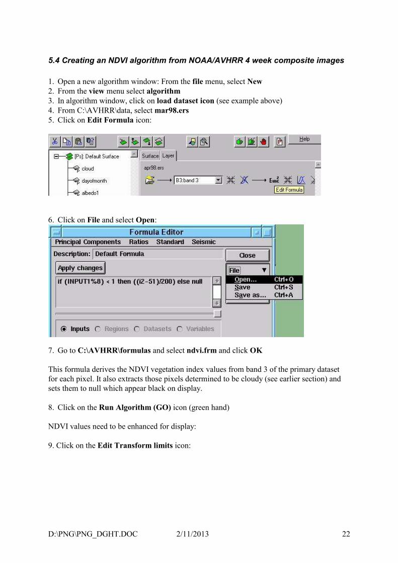
5.4 Creating an NDVI algorithm from NOAA/AVHRR 4 week composite images
1. Open a new algorithm window: From the file menu, select New
2. From the view menu select algorithm
3. In algorithm window, click on load dataset icon (see example above)
4. From C:\AVHRR\data, select mar98.ers
5. Click on Edit Formula icon:
6. Click on File and select Open:
7. Go to C:\AVHRR\formulas and select ndvi.frm and click OK
This formula derives the NDVI vegetation index values from band 3 of the primary dataset
for each pixel. It also extracts those pixels determined to be cloudy (see earlier section) and
sets them to null which appear black on display.
8. Click on the Run Algorithm (GO) icon (green hand)
NDVI values need to be enhanced for display:
9. Click on the Edit Transform limits icon:

D:\PNG\PNG_DGHT.DOC 2/11/2013 23
10. Click on Limits and select Limits to Actual
11. Click on the Run Algorithm (GO)
12. Manipulate transform breakpoints to adjust display colours
13. From the algorithm window select surface and then Color Table - Experiment with
look up tables.

D:\PNG\PNG_DGHT.DOC 2/11/2013 24
5.5 Using the AGSO/CSIRO ER-Mapper algorithm system developed at the PNGGS
Fig. 9 shows how the files are structured to create display and printing algorithms for 4 and 8-
week composites and difference images. This is done through a series of Ermapper virtual
datasets and algorithms. Formulas for the various steps are embedded in the files.
Because 8-week composite images require a specific data value for cloud areas a new dataset
(not virtual) must be created from the primary data sets. To use all the 8-week algorithms and
data, the dataset allreal.ers and allreal must be loaded from CD # 3.
ALL8WK.ALG
C:\AVHRR\ALGS
8WKREALV.ERS
C:\AVHRR\DATA
ALL4WK.ALG
C:\AVHRR\ALGS
4WKDIFF.ALG
C:\AVHRR\ALGS
8WKDIFF.ERS
C:\AVHRR\DATA
8WKNDVI
C:\AVHRR\ALGS\
PRINTALG
8WKDIFF
C:\AVHRR\ALGS\
PRINTALG
4WKNDVI
C:\AVHRR\ALGS\
PRINTALG
4WKDIFF
C:\AVHRR\ALGS\
PRINTALG
SOURCE DATADISPLAY ALGORITHMS &VIRTUAL DATA SETS
PRINTALGORITHMS
CD #3
CD #4
96CD.ALG
C:\AVHRR\ALGS
97CD.ALG
C:\AVHRR\ALGS
ALLREAL.ERS
CD #3 &
C:\AVHRR\DATA
4WKNEW_V.ERS
C:\AVHRR\DATA
4WKNEW.ERS
C:\AVHRR\DATA
Fig. 9: Flow chart of file structure.

D:\PNG\PNG_DGHT.DOC 2/11/2013 25
5.5.1 Creating a data-set for new AVHRR data
1. From the file menu select Open from Virtual Dataset
2. Go to C:\AVHRR\data and select 4wknew_v
This is a virtual dataset to be added to containing the march98 dataset
3. From the view menu, select algorithm
4. Click on the duplicate icon:
5. Click on Load Dataset
6. Select file from C:\AVHRR\data, e.g.apr98.ers and OK this layer only
7. Make sure all layers are turned on and rename the bottom layer on the left-hand side from
mar98 to the new name.
8. Click on the Run Algorithm (GO) icon (green hand)
9. Click on the Edit Transform limits icon:
10. Click on the Limits button and then select Limits to actual:

D:\PNG\PNG_DGHT.DOC 2/11/2013 26
11. Click on the Limits button and then select Set Output Limits to Input Limits (this
ensures that clouds are saved as a data value of -9999).
12. From the file menu, select Save as Virtual Dataset
13. Save as 4wknew_v.ers
14. From the file menu, select Save as Dataset
15. In the Save as Dataset window choose the following:

D:\PNG\PNG_DGHT.DOC 2/11/2013 27
5.5.2 Adding to and creating 4 week composite display and printing algorithms.
1. From the file menu select Open
5. From C:\AVHRR\algs, select all4wk.alg
6. From the menu above, select view then algorithm
7. Click on the Duplicate icon
8. Click on Load Dataset
9. Choose C:\AVHRR\data\4wknew.ers
10. Load desired monthly NDVI data e.g. apr98:
11. Change layer name to new name, eg apr98
12. Turn other layers off with the Turn On/Off icon
13. From the file menu, select Save as
14. C:\AVHRR\algs\all4wk.alg
15. Click yes to overwrite the file (original algorithms can be found in C:\AGSO\algs)
16. From the file menu, select Save as
17. Go to C:\AVHRR\algs\printalg\4wkndvi
18. Save as filename, eg apr98.alg

D:\PNG\PNG_DGHT.DOC 2/11/2013 28
5.5.3 Adding to and creating 4- week difference image display and printing algorithms.
1. From the file menu select Open
2. From C:\AVHRR\algs, select 4wkdiff.alg
3. From the menu above, select view then algorithm
4. Click on the Duplicate icon
5. Click on Load Dataset
6. Choose C:\AVHRR\data\4wknew.ers and OK this layer only
7. Load desired monthly NDVI data for differencing e.g. mar98 and apr98 to subtract
apr98 from mar98:
1. Change layer name to new name, eg marapr98
2. Turn other layers off with the Turn On/Off icon
Note: It is important not to change the transform for one image only as this is used as a
standard for image comparisons.
3. From the file menu, select Save as
4. C:\AVHRR\algs\4wkdif.alg
5. Click yes to overwrite the file (original algorithms can be found in C:\AGSO\algs)
6. From the file menu, select Save as
7. Go to C:\AVHRR\algs\printalg\4wkdiff
8. Save as filename, eg marapr98.alg

D:\PNG\PNG_DGHT.DOC 2/11/2013 29
5.5.4. Adding to and creating 8-week composite display and printing algorithms.
1. From the file menu select Open
2. From C:\AVHRR\algs, select all8wk.alg
3. From the menu above, select view then algorithm
4. Turn all layers off and go to the bottom 8 week layer, eg janfeb98
5. Click on the Duplicate icon
6. Click on Load Dataset
7. Choose C:\AVHRR\algs\4wknew.ers
8. Load desired monthly NDVI data for 2 month composites e.g. mar98 and apr98 to
composite apr98 and mar98. The formula is set up so that the highest NDVI value is
taken so that there is less cloud than in the individual months.
9. Change layer name to new name, eg marapr98
10. From the file menu, select Save as
11. C:\AVHRR\algs\all8wk.alg
12. Click yes to overwrite the file (original algorithms can be found in C:\AGSO\algs)
13. From the file menu, select Save as
14. Go to C:\AVHRR\algs\printalg\8wkndvi
15. Save as filename, eg marapr98.alg
5.5.5 Adding to and creating 8-week difference image display and printing algorithms.
5.5.5.1. Adding to the 8 week composite virtual data-set
1. From the file menu select open from virtual data-set
2. Go to C:\AVHRR\data and select 8wkrealv.ers
3. From the menu above, select view then algorithm
4. Go to the bottom 8 week layer, eg janfeb98
5. Click on the Duplicate icon
6. Click on Load Dataset
7. Choose C:\AVHRR\algs\4wknew.ers
8. Load desired monthly NDVI data for 2 month composites e.g. mar98 and apr98 to
composite apr98 and mar98. The formula is set up so that the highest NDVI value is
taken so that there is less cloud than in the individual months.
9. Change layer name to new name, eg marapr98
10. From the file menu, select Save as Virtual Dataset
11. C:\AVHRR\algs\8wkrealv.ers
12. Click yes to overwrite the file (original algorithms can be found in C:\AGSO\algs)

D:\PNG\PNG_DGHT.DOC 2/11/2013 30
5.5.5.2. Adding to the 8 week difference algorithm
1. From the file menu select Open
2. From C:\AVHRR\algs, select 8wkdiff.alg
3. From the menu above, select view then algorithm
4. Turn all layers off and go to the bottom 8 week layer, eg novdec97-janfeb98
5. Click on the Duplicate icon
6. Load desired monthly NDVI 2 month composites e.g. janfeb98 and marapr98 to produce
a difference. The formula is set up so that marapr98 will be subtracted from janfeb98.
7. Change layer name to new name, eg janfeb-marapr98
8. From the file menu, select Save as
9. C:\AVHRR\algs\8wkdiff.alg
10. Click yes to overwrite the file (original algorithms can be found in C:\AGSO\algs)
11. From the file menu, select Save as
12. Go to C:\AVHRR\algs\printalg\8wkndvi
13. Save as filename, eg jf98-ma98.alg

D:\PNG\PNG_DGHT.DOC 2/11/2013 31
5.6 Making a poster algorithm
1. Open a new algorithm window: From the file menu, select New
2. From the view menu select algorithm
3. In Algorithm window click on Edit and then Add Vector Layer, then Annotation Map
Composition:
4. Click on Load Dataset icon
5. Go to C:\avhrr\vectors and select a .erv file. Eg. 8wkdiff.erv
6. Click on Annotate Vector Layer icon:
7. Tool icons appear. Click on Select and Move/Resize Mode
8. Double click on any square in the image

D:\PNG\PNG_DGHT.DOC 2/11/2013 32
Map Object Attributes and Map Object Select boxes appear. Make sure that Map Object
Select Category equals Algorithm
9. Click on Open Dataset icon next to Algorithm Name:
10. Load algorithm to be displayed in selected box. 4 week NDVI data, for example, can be
loaded from C:\AVHRR\algs\printalg\4wkndvi
11. Select Close on Tools icon bar
12. Save the vector file
13. Select Save as from the File menu and save the algorithm.
Image boxes can be resized to fit the image and text can be added in this or another
annotation layer. It may be difficult to print a large poster file as large amounts of disk space
are required to create a temporary postscript file. One way to get around this is to print to a
file:
14. From the file menu choose print
15. In the print window, load the algorithm and choose the output name ER_Mapper.hc

D:\PNG\PNG_DGHT.DOC 2/11/2013 33
16. Select hardcopy control Files and fit page to output device
17. Click on Setup;
18. Type pathname to dataset in Filter Program
19. Insert appropriate image dimensions in Page dots across and down, e.g, 2000 x 2500.
20. Click Ok, then Print
The resulting dataset will be 3 band and can be printed when loaded into a standard RGB
algorithm
D:\PNG\PNG_DGHT.DOC 2/11/2013 34
6.0 Analysis of the Remotely Sensed Imagery
6.1 Initial Analysis and Visualization of PNG_DATS
After visually inspecting the different composite images purchased from CSIRO Marine
Research Hobart, it was decided that too much cloud was present in the 2-week AVHRR
composite for it to be of use in the time series analysis. Consequently, in June 1998 it was
recommended to CSIRO Marine Research that 2-week composites for PNG not be produced
in the future.
Posters for 4-week data were produced in ER-Mapper, (Fig. 7 and Section 5.6). Visual
analysis of the 4-week AVHRR composite data led to a decision to create 8-week composites
(Fig. 8 and Section 5.6). These provided promising images.
A difference image is calculated by subtracting the values of one image from another image
(Fig. 10 fold out). If there is null data (due to cloud cover) in either image, then this is null in
the resulting difference image. Fig. 10a is the 8-week composite data for Sept/Oct period and
Fig. 10b is the 8-week composite data for Nov/Dec period. These are the two input images
and high NDVI values in both are coloured red and low NDVI values are coloured blue. Fig.
10c is the difference image, red areas indicate a decrease in the NDVI value between the two
images and blue areas an increase in the NDVI between the two times. Drought and the
associated decrease in vegetation cover is one reason why the NDVI would decrease through
time. There are several other factors which causes change in the NDVI signal these include
land cover changes and that cloud flagging algorithms may not have sucessfully identified all
cloud affected pixels, especially sub-pixel cloud. For example, in Fig. 10c in New Britain
some of the small areas where there NDVI values has decreased quickly (the small red areas)
may be due to logging operations (McAlpine pers. comm.). Field assessments would be
needed to confirm this. Also in Fig 10c in Western Province the complex patterns of a high
increases and decreases in NDVI are probably due to complex hydrology of that area
(Bellamy, 1995).
When dealing with a time series of images it is possible to monitor the trends though time
(e.g. time1 minus time2; time2 minus time3; time3 minus time4, and so on). To highlight
changes in the NDVI signal between consecutive images, difference images were calculated
for both the 4-week composite and 8-week composite data (Fig. 11 and 12, respectively both
are fold outs). Fig. 12 shows the relative stability of the NDVI signal during 1996 and that
there is a large decrease in various locations for different times in the later half of 1997. An
increase of the NDVI values, which may be interpreted as a recovery from the drought event
is illustrated late in 1997 (Fig. 12). Whether this actually constitutes recovery depends on the
definition of drought and may be seen as precurrsive to the subsistence-based agricultural
communities having access to normal food supplies. To confirm that food production has
returned to normal levels field surveys must be undertaken (Allen and Bourke, 1997, Allen,
1998). Fig. 11 (4-week data) shows a similar trend to Fig. 12 (8-week data). While there is a
higher temporal resolution in the 4-week data, there is more cloud present when compared to
the 8-week data (Figs 11 and 12).

D:\PNG\PNG_DGHT.DOC 2/11/2013 35
The mean NDVI and Ts were calculated from the 8-week AVHRR composites for the PNG
land area. The mean Ts increases slightly earlier than the mean NDVI decreases at the height
of the 1997 drought event; which occurred in the later half of 1997 (Fig. 13.1). In the early
part of 1997 the mean NDVI actually increases. During 1996, a year which received average
rainfall, the NDVI also increased slightly early in the year. However, these perturbations are
minor compared to the large increase in Ts and decrease in NDVI associated with the 1997
drought event (Fig. 13.1). The date for each composite image plotted on the x-axis of the time
series plot is the central date of the composite period.
To provide a finer time step when focusing on drought onset and recovery we explored the
use of the 4-week composite data from 1997. Using a longer composite period causes the
amplitude in the signal of NDVI and Ts to be dampened (compare Figs 13.1 and 13.2). Based
on these results we decided to use the 8-week AVHRR data for 1996 and the 4-week data for
1997 and 1998. This pragmatic approach uses AVHRR data with a shorter composite period,
when low amounts of cloud cover existed due to drought. An analysis over a longer time
period of the drought recovery phase may require using 8-week composite data during 1998.
During Jan97 and Feb97 AVHRR data collected had high amounts of cloud contaminated
pixels. The percentage of valid data for the 4-week composites during the rest of 1997 is
similar to that for the 8-week composite data (Fig. 14.1 and 14.2).
Fig. 13.1 shows that local maxima of Ts coincide with the equinox (March and September)
for both 1996 and 1997. This is due to increased solar loading at these times in equatorial
countries, like PNG. The Normalised Difference Temperature Index (NDTI), jointly
developed by McVicar et al. (1992) and Jupp et al. (1998), provides a means to normalise for
both daily (changes in atmospheric transmittance) and seasonal (earth-sun distances)
influences of net radiation. The NDTI requires daily rainfall and extremes of air temperature;
this daily meteorological data was not available for this study. During 1997 both Figs 13.1
and 13.2 show a lag between the time of maximum Ts and the time of minimum NDVI. This
pattern is due to Ts being influenced by both net radiation and available soil moisture and the
NDVI reflecting a lag between vegetation response of conditions (Goetz, 1997). The NDTI
provides a method for separating the influence of net radiation and moisture availability in Ts.
McVicar and Jupp (1998) suggest that using the resource availability and resource utilisation
can be mapped using the NDTI and NDVI, respectively.

D:\PNG\PNG_DGHT.DOC 2/11/2013 36
Fig. 13.1 and 13.2 show that Ts and NDVI are negatively correlated. Many previous
researchers have related this to estimating ET, partitioning of energy balance components,
estimation of surface moisture status and land cover classification. General applications of the
combined use of Ts and NDVI are referred to by Goetz (1997); and for discussion of the
combined use of Ts and NDVI relevant to drought refer to McVicar and Jupp (1998). Goetz

D:\PNG\PNG_DGHT.DOC 2/11/2013 37
(1997) reported that the negative correlation between Ts and NDVI, observed at several
remotely sensed scales (25 m2 to 1.2 km
2), was largely due to changes in vegetation cover and
soil moisture. Held et al. (1995) used a ratio of Ts/NDVI as the spatial backbone to
extrapolate a single ground based measurement of ET to a LANDSAT TM quarter scene (90
km2). For complete canopies, the slope of the Ts/NDVI relationship has been related to
canopy resistance (Nemani and Running, 1989, Sellers, 1987, Hope, 1988). Nemani et al.
(1993) found the slope of Ts/NDVI to be negatively correlated to crop-moisture index.
Currently, advances are being made that use the Ts/NDVI plot, combined with meteorological
data and process based models to provide a more mechanistic interpretation of the remotely
sensed data. There are two methods currently being put forward. The first, is a progression
from the slope of Ts/NDVI approach, which describes the data as falling into a triangle
(Gillies and Carlson, 1995, Gillies et al., 1997, Carlson et al., 1990, Carlson et al., 1994,
Price, 1990). The second, the Vegetation Index / Temperature Trapezoid (VITT) (Moran et
al., 1994, Moran et al., 1996, Yang et al., 1997), is an evolution of the Crop Water Stress
Index (CWSI), which promotes the idea of data falling into a trapezoid. Both of these
techniques require ancillary meteorological data to spatially distribute inferences about the
surface energy balance fluxes, or moisture availability. Full descriptions of each of these
approaches, and their advantages and disadvantages for operational drought assessment are
given in a review by McVicar and Jupp (1998).
For this study in PNG, which was aimed at providing a rapid assessment of the 1997 drought
conditions, daily meteorological data was not available. Consequently we had to develop a
system which could be based primarily on remotely sensed data. To perform this, and to utlise
the negative correlation between Ts and NDVI data, we divided Ts by NDVI. This ratio
(Ts/NDVI) becomes higher during times of stress, due to the decrease in NDVI associated
with lower plant cover, and the increase in Ts associated with more of the ground surface
available energy being partitioned into the sensible heat flux (Fig. 15.1 and 15.2). The time
series of Ts/NDVI is an indicator of environmental stress, associated with the 1997 drought
conditions in PNG. It does not attempt to provide estimates of the Bowen ratio (the ratio of
the sensible heat flux divided by the latent energy heat flux) or provide an input parameter to
regional ET modelling.
Longer composite periods dampens the signal of the Ts/NDVI ratio. To observe this
dampening effect, compare 1997 in Fig. 15.1 (8-week composites) with 1997 in Fig. 15.2 (4-
week composites). In both Fig. 15.1 and 15.2 there is an increase in Ts/NDVI associated with
the 1997 drought event. However, in Fig. 15.2 the increase of Ts/NDVI is larger. This
increase results because composites are formed based on the maximum NDVI during the
period (Section 4.1). Consequently a shorter composite period (in which a lower NDVI data
that is cloud free is acquired) means that higher Ts/NDVI values associated with the 1997
drought in PNG will be observed.
During the height of the drought an individual cloud free image may have been acquired
which had lower NDVI value than the image used in the composite. However, due to
compositing based on the maximum NDVI, this hypothetical image would not be used in the
composite. This means that there may be an individual image with a higher Ts/NDVI ratio
than is presented here using the composite data.
The next task was to asses differences in the intensity and timing of the 1997 drought event,
as monitored by the Ts/NDVI ratio, for different regions within PNG. The regions selected
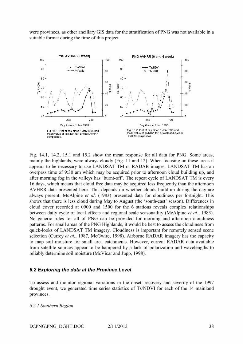
D:\PNG\PNG_DGHT.DOC 2/11/2013 38
were provinces, as other ancillary GIS data for the stratification of PNG was not available in a
suitable format during the time of this project.
Fig. 14.1, 14.2, 15.1 and 15.2 show the mean response for all data for PNG. Some areas,
mainly the highlands, were always cloudy (Fig. 11 and 12). When focusing on these areas it
appears to be necessary to use LANDSAT TM or RADAR images. LANDSAT TM has an
overpass time of 9:30 am which may be acquired prior to afternoon cloud building up, and
after morning fog in the valleys has ‘burnt-off’. The repeat cycle of LANDSAT TM is every
16 days, which means that cloud free data may be acquired less frequently than the afternoon
AVHRR data presented here. This depends on whether clouds build-up during the day are
always present. McAlpine et al. (1983) presented data for cloudiness per fortnight. This
shows that there is less cloud during May to August (the ‘south-east’ season). Differences in
cloud cover recorded at 0900 and 1500 for the 6 stations reveals complex relationships
between daily cycle of local effects and regional scale seasonaility (McAlpine et al., 1983).
No generic rules for all of PNG can be provided for morning and afternoon cloudiness
patterns. For small areas of the PNG Highlands, it would be best to assess the cloudiness from
quick-looks of LANDSAT TM imagery. Cloudiness is important for remotely sensed scene
selection (Currey et al., 1987, McGwire, 1998). Airborne RADAR imagery has the capacity
to map soil moisture for small area catchments. However, current RADAR data available
from satellite sources appear to be hampered by a lack of polarization and wavelengths to
reliably determine soil moisture (McVicar and Jupp, 1998).
6.2 Exploring the data at the Province Level
To assess and monitor regional variations in the onset, recovery and severity of the 1997
drought event, we generated time series statistics of Ts/NDVI for each of the 14 mainland
provinces.
6.2.1 Southern Region

D:\PNG\PNG_DGHT.DOC 2/11/2013 39
There are five provinces which comprise the Southern Region. These are Western, Gulf,
Central, Milne Bay and Northern (Fig. 1). Western Province (Fig. 16.1) was the worst
affected province, as measured by the Ts/NDVI ratio. Central Province (Fig. 16.3) was also
badly affected by the 1997 drought event. During 1997 it appears that Milne Bay (Fig. 16.4)
may have suffered a longer period of dry conditions compared with the response recorded for
Gulf Province (Fig. 16.2). This agrees with the finding of of ground based drought assessment
(Allen et al., 1997).
Milne Bay Province (Fig. 16.4) also experienced a slight increase in stress in the middle of
1996, a year during which most of PNG received average rainfall. The increase in Ts/NDVI
for Milne Bay Province for 1996 may be associated with marked rainfall seasonality.
Frequently small perturbations of Ts/NDVI occur when the proportion of valid data for the
province decreases below 10%. This can especially be seen in the plot for Northern Province
(16.5). For the first year of data, the ratio is fairly stable (indicating that drought conditions
were not experienced during that year as average rainfall was received in 1996) and the
proportion of valid data is generally larger than 30%. However, early in the second year of
analysis, a small decrease can be seen associated with a very low proportion of valid data for
that province. When the proportion of valid data is low for other Southern Provinces small
perturbations can also be seen.
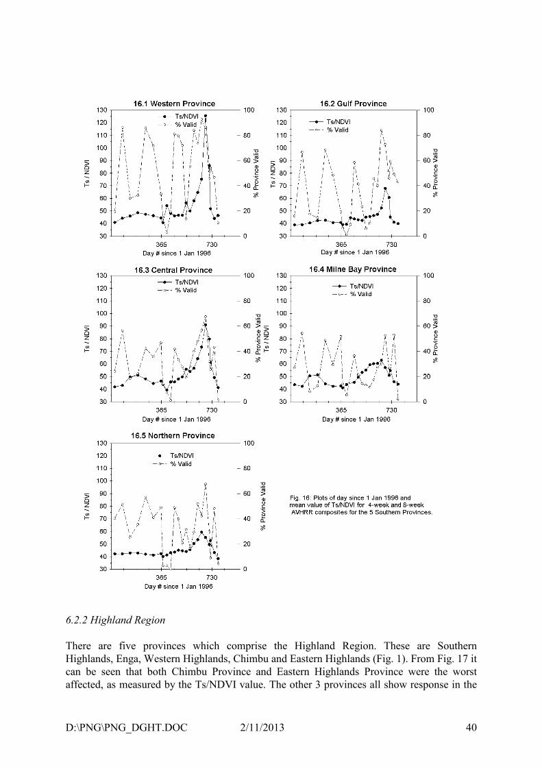
D:\PNG\PNG_DGHT.DOC 2/11/2013 40
6.2.2 Highland Region
There are five provinces which comprise the Highland Region. These are Southern
Highlands, Enga, Western Highlands, Chimbu and Eastern Highlands (Fig. 1). From Fig. 17 it
can be seen that both Chimbu Province and Eastern Highlands Province were the worst
affected, as measured by the Ts/NDVI value. The other 3 provinces all show response in the

D:\PNG\PNG_DGHT.DOC 2/11/2013 41
Ts/NDVI ratio during the 1997 drought event. For all of the Provinces there is a slight
increase in the Ts/NDVI ratio during August - November 1996. Rainfall seasonality
experienced in the provinces is primarily a Jan-Apr maxima (McAlpine, 1995), which agrees
with the trends shown in Fig. 17. It is also interesting to note that for Eastern Highlands
Province the base value of Ts/NDVI is higher when compared to the other 4 Highland
Provinces. This indicates that this province generally receive less rainfall than the other
Highland Provinces (Bourke, 1988). The increase is stress, revealed by the baseline during
1996 of Ts/NDVI and by the magnitude of the ratio during 1997 for both Eastern Highlands
Province and Chimbu Province is confirmed by the rainfall being lower in the eastern
Highlands and tending to increase in a westerly direction (Bourke, 1988, p.10). The main
other environmental factors which could control this response soils (mainly ash) and
topography (ranging from flat valley to very steep slopes) are generally the same over the
entire highland region (Bourke pers. comm.).

D:\PNG\PNG_DGHT.DOC 2/11/2013 42
6.2.3 Mamose Region
There are four provinces which comprise the Mamose Region. These are Morobe, Madang,
East Sepik and West Sepik (Fig. 1). Morobe Province (Fig. 18.1) suffered a more intense (the
Ts/NDVI value was higher) and longer (the Ts/NDVI value is higher than 50 for a longer

D:\PNG\PNG_DGHT.DOC 2/11/2013 43
period) drought in 1997 than the other provinces in this region. Madang (Fig. 18.2)
experienced stress, due to the 1997 drought, as indicated by the Ts/NDVI value increasing
sharply in the later half of 1997. East Sepik Province (Fig. 18.3) was moderately affected, and
West Sepik Province (Fig. 18.4) only slightly influenced, by the 1997 drought, as measured
by the Ts/NDVI ratio. This agrees with the finding of of ground based drought assessment
(Allen et al., 1997).
6.2.4 Provinces of Interest
The vast differences in the response of Ts/NDVI for 4 provinces of interest is shown in Fig.
19. From this plot it can be seen that Western Province experienced the most intense drought
during 1997 (Fig. 19.1). Milne Bay Province (Fig. 19.2) suffered a prolonged period in 1997
where dry conditions occurred. However, Milne Bay Province also seemed to have
experienced a dry period in 1996, which may have been associated with rains occurring late
in the May-August rainfall maxima (McAlpine, 1995). East Highlands Province (Fig. 19.3)
experienced drought in 1997 as indicated by the long period when the Ts/NDVI signal is

D:\PNG\PNG_DGHT.DOC 2/11/2013 44
high. West Sepik Province (Fig. 19.4) did not experience severe drought conditions in 1997,
demonstrated by the low values of the Ts/NDVI signal.
6.3 Combining the data with meteorological data sets
Monthly rainfall recorded at the meteorological stations shown in Fig. 1 was available from
Jan 1997 until April 1998. However, during this period not all stations had complete monthly
rainfall records. Several of the stations that experienced severe drought conditions, not
providing data (Miaha pers. comm). This provides strong support for field visits and the use
of remotely sensed data to assess the drought conditions. At the meteorological stations we
were able to extract the Ts/NDVI values for an area 99 by 99 pixels, with the station being
centrally in this area.
Fig. 20.1, 21.1 and 22.1 are plots of Ts/NDVI (left hand Y-axis) for the area surrounding the
station and monthly rainfall (right hand Y-axis) against time for Kiunga, Wewak and Nadzab,
respectively. The plots show that Kiunga received more rainfall than Wewak and Nadzab
during 1997. The integral under the plot of Ts/NDVI is a reciprocal of this. Figs 20.2, 21.2

D:\PNG\PNG_DGHT.DOC 2/11/2013 45
and 22.2 are plots of Ts/NDVI (left hand Y-axis) for the area surrounding the station and
percent monthly average rainfall (right hand Y-axis) against time. These plots do not show
the same strong relationship as the monthly rainfall plots.

D:\PNG\PNG_DGHT.DOC 2/11/2013 46
7.0 Recommendations: Opportunities & Improvements
7.1 Opportunities
There are a number of opportunities which would allow full use of the composite AVHRR
data for assessment and monitoring of the 1997 PNG drought situation. These are:
• Assessing the recovery phase of the drought during 1998 would be achieved by comparing
the satellite data from 1998 with that recorded in 1996. UNDP have already committed
funds for the project to purchase AVHRR composite data from CSIRO Marine Research in
Hobart until the end of 1998. What is needed is the opportunity to allow analysts from
PNG and Australia to work together to fully explore this.
• Working more closely with staff, with the appropriate technical skills (remote sensing and
spatial information) and discipline training (agriculture), from PNG Department of
Agriculture and Livestock would be of value. To date PNG_DATS has been installed in
PNGGS, where they have ER-Mapper, the image processing system that the analysis is
built around. It would be useful if PNG Department of Agriculture and Livestock also had
ER-Mapper. Selected staff within the Department would require training for the package.
An advantage of using ER-Mapper as the basis for PNG_DATS is that images do not need
to be stored on disk after every processing option. Having “virtual datasets” greatly
reduces the need for large hard disk space. Currently each of the 4-week composite images
are 22 Megabytes (Mb) and over the three years there will be 39 base images in the time
series. This totals 858 Mb of base data. If another image processing system was installed at
PNG Department of Agriculture and Livestock then disk space would become an issue and
large disks would be required.

D:\PNG\PNG_DGHT.DOC 2/11/2013 47
• If would be beneficial to have access to a map, in digital format, of agricultural regions.
Currently such exists with DAL, however due to a number of reasons including computer
networking, we could access this for PNG_DATS which is currently located at PNGGS. If
we could get access to this map this would allow analysis to be performed for only
agricultural areas within each province. This level of detail would have been more useful
to assess the drought situation for different agricultural production systems.
• A post-graduate degree candidate, possibly from within PNG Department of Agriculture,
could fully establish the reasons for different responses within the context of the PNG
1997 drought. There is the opportunity to assess how to use remotely sensed data (which
does not cover all of PNG area due to clouds) with generated surfaces of rainfall. It may be
appropriate that this person be enrolled with ANU CRES and have contact with AGSO
and CSIRO Land and Water staff.
Independent of the AVHRR time series data set developed here there are several
opportunities that may in increase the understanding of drought in PNG. These are:
• Of direct relevance to developing a system for early prediction of drought in PNG Nicholls
(1973) showed that weakened “Walker Circulation” sometimes corresponds to severe
droughts in PNG. More recently, in Australia, rainfall (McBride and Nicholls, 1983,
Nicholls, 1989) and crop yields of sorghum (Nicholls, 1986) and wheat (Rimmington and
Nicholls, 1993) have been related to the El Niño Southern Oscillation (ENSO). ENSO can
be thought of as a refinement of the weakened “Walker Circulation” introduced by
(Nicholls, 1973). Examining historical trends of ENSO and drought occurrence in PNG
may provide a drought early warning system. Some rules may be developed, possibly
based on a combination of the magnitude, rate of change and the timing of the ENSO
signal to indicate that PNG may soon experience drought conditions. When these
hypothetical rules are met, it may be necessary to monitor both ground based
meteorological data and hi-frequency remotely sensed data, as introduced in this report, to
monitor development of the potential drought conditions. Ground based rainfall data can
be in a root crop water balance model, with some probabilities of future rainfall amounts,
to provide estimates of when crop failure may occur up to 8 weeks prior to the actual event
(McApline pers. comm.). Southern Oscillation Index (SOI), which is based upon air
pressure difference between Darwin and Tahiti provides a means of tracking changes in
ENSO. SOI values can be obtained from the following WWW address:
http://www.BoM.GOV.AU/climate/current/soihtm1.shtml
• In the Highlands, during the height of the drought, frost mapping could be attempted using
night time thermal GMS data, which is recorded at hourly intervals. This could be
combined with a DEM (to determine possible paths of cold air drainage) and maps of
population distribution. This may show where drought affected the food supply to the
subsistence based agricultural communities. This remote and synoptic study, would have
to be validated by on ground field studies. Fig. 23 illustrates the type data visulation that
can be performed when there is access to a DEM.
7.2 Recommended Future Improvements

D:\PNG\PNG_DGHT.DOC 2/11/2013 48
Some improvements would have greatly helped in the establishment, transfer and analysis of
PNG_DATS.
• At present the AVHRR composite period is 4-week. It would be preferable if the data was
monthly (that is a composite period from the 1st of each month until the last day of the
month). Monthly composites would allow easier transfer and extension to agricultural and
relief staff. This may be accomplished by CSIRO Marine Research reprocessing the data to
these periods. If that data is reprocessed, there is the opportunity to have digital data over
the ocean parts of the image, not just the land. This may allow other applications to make
use of this time series of AVHRR data.
• Access to ancillary digital data covering all of PNG would have been useful for the
analysis within PNG_DATS. Possible sources of ancillary data could include PNGRIS, the
digital elevation model (DEM) recently delivered to PNG DEC, and the improved
vegetation polygons. The vegetation polygons required for this study would be based on a
broad level of classification (not species or harvestable volumes) present in the PNG
Forestry Authority Forest Information System (FIM). At the PNG Departmental level data
custodian and transfer agreements are currently being addressed. Having an established
protocol and point of contact for various data sets would have been extremely useful to
this project.
8.0 Conclusions
Composite AVHRR imagery can be used to assess and monitor drought development and
recovery in PNG. Cloud is a problem in PNG for reflective and thermal remotely sensed data,
however, useful information was gained from this data set.
Transforming the AVHRR to the Ts/NDVI ratio provided a direct measure of environmental
stress. This does not require ancillary meteorological data, and may be a useful data
transformation to monitor drought conditions in other countries and regions. The Ts/NDVI
ratio can be obtained from remotely sensed data alone. Not requiring ancillary ground based
meteorological data may be an advantage for other countries.
9.0 Acknowledgments
This project was funded by the Papua New Guinea office of the United Nations Development
Program (UNDP). Thanks are extended to all who willingly provided help and assistance in
getting the project going in a short time frame. Paul Tildesley and Kim Badcock processed
the AVHRR time series data base that was central to the project. Sam Maiha provided
monthly rainfall data. AGSO SIMS staff (Ross Hill and Chris Fitzgerald) produced figures
and the associated poster, CSIRO Land and Water staff (Heinz Buettikofer and Tony
Tatarow) also produced some of the figures. Thanks are extended to all for wonderful
graphics. Jim Mollison, ACRES, clarified RADAR data acquisition over PNG. Thanks to Drs
D:\PNG\PNG_DGHT.DOC 2/11/2013 49
Bryant Allen, Mike Bourke, Alex Held, Gerry Jacobson, and John McAlpine for reviewing
and making suggestions on an earlier draft that improved this final version.
10.0 References
Allen, B. (1989). Frost and Drought Through Time and Space, Part I: The Climatological
Record. Mountain Research and Development, 9, 252-278.
Allen, B., Brookfield, H. and Byron, Y. (1989). Frost and Drought Through Time and Space,
Part II: The Written, Oral, and Proxy Records and their meaning. Mountain Research
and Development, 9, 252-278.
Allen, B.J. (1998). The 1997-98 Papua New Guinea Drought: Perceptions of Disaster. The
Australian Centre for International and Tropical Health and Nutrition, University of
Queensland, Brisbane, pp. 14.
Allen, B.J. and Bourke, R.M. (1997). Report of an Assessment of the Impacts of Frost and
Drought in Papua New Guinea. Papua New Guinea Department of Provincial and
Local Government Affairs, Canberra, pp. 20.
Allen, B.J., Bourke, R.M., Burton, J., Flew, S., Gaupu, B., Heia, S., Igua, P., Ivahupa, S.,
Kanua, M., Kokoa, P., Lillicrap, S., Ling, G., Lowe, M., Lutulele, R., Nongkas, A.,
Poienou, M., Risimeri, J., Sheldon, R., Sowei, J., Ukegawa, K., Willson, N., Wissink,
D. and Woruba, M. (1997). Report of an Assessment of the Impacts of Frost and
Drought in Papua New Guinea - Phase 2. Papua New Guinea Department of
Provincial and Local Government Affairs, Canberra, pp. 27.
Alley, W.M. (1984). The Palmer Drought Severity Index: Limitations and Assumptions.
Journal of Climate and Applied Meteorology, 23, 1100-1109.
Alley, W.M. (1985). The Palmer Drought Severity Index as a Measure of Hydrologic
Drought. Water Resources Bulletin, 21, 105-114.
Bellamy, J.A. (1995). Landform Type. In Papua New Guinea Inventory of Natural Resources,
Population Distribution and Land Use Handbook, Vol. 6 (Eds, Bellamy, J. A. and
McAlpine, J. R.) AusAID, Canberra, pp. 162.
Bourke, R.M. (1988). Taim hangre: variation in subsistence food supply in the Papua New
Guinea highlands. In Department of Human Geography Australian National
University, Canberra.
Bourke, R.M. (1989). The Influence of Soil Moisture on Sweet Potato Yield in the Papua
New Guinea Highlands. Mountain Research and Development, 9, 322-321.

D:\PNG\PNG_DGHT.DOC 2/11/2013 50
Bourke, R.M. (1998). Impact of the 1997 drought and frosts in Papua New Guinea. The
Australian Centre for International and Tropical Health and Nutrition, University of
Queensland, Brisbane, pp. 10.
Brookfield, H. and Allen, B. (1989). High-Altitude Occupation and Environment. Mountain
Research and Development, 9, 201-209.
Burgess, W. and Pairman, D. (1997). Bidirectional reflectance effects in NOAA AVHRR
data. International Journal of Remote Sensing, 18, 2815-2825.
Carlson, T.N., Gillies, R.R. and Perry, E.M. (1994). A method to make use of thermal
infrared temperatures and NDVI measurements to infer soil water content and
fractional vegetation cover. Remote Sensing Reviews, 9, 161-173.
Carlson, T.N., Perry, E.M. and Schmugge, T.J. (1990). Remote Estimation of Soil Moisture
Availability and Fractional Vegetation Cover for Agricultural Fields. Agricultural and
Forest Meteorology, 52, 45-69.
Choudhury, B.J. and DiGirolamo, N.E. (1995). Quantifying the Effect of Emissivity on the
Relation between AVHRR Split Window Temperature Difference and Atmospheric
Precipitable Water over Land Surface. Remote Sensing of Environment, 54, 313-323.
Cognard, A.-L., Loumagne, C., Normand, M., Olivier, P., Ottle, C., Vidal-Madjar, D.,
Louahala, S. and Vidal, A. (1995). Evaluation of the ERS1 synthetic aperture radar
capacity to estimate surface soil moisture: Two-year results over the Naizin
watershed. Water Resources Research, 31, 975-982.
Currey, B., Fraser, A.S. and Bardsley, K.L. (1987). How useful is Landsat monitoring?
Nature, 328, 587-589.
Deering, D.W. (1989). Field Measurements of Bidirectional Reflectance. In Theory and
Application of Optical Remote Sensing(Ed, Asrar, G.) John Wiley and Sons, New
York, pp. 14-65.
Gillies, R.R. and Carlson, T.N. (1995). Thermal remote sensing of surface soil water content
with partial vegetation cover for incorporating into climate models. Journal of Applied
Meteorology, 34, 745-756.
Gillies, R.R., Carlson, T.N., Cui, J., Kustas, W.P. and Humes, K.S. (1997). A verification of
the ‘triangle’ method for obtaining surface soil water content and energy fluxes from
the remote measurements of the Normalized Difference Vegetation Index (NDVI) and
surface radiant temperature. International Journal of Remote Sensing, 18, 3145-3166.
Goetz, S.J. (1997). Multi-sensor analysis of NDVI, surface temperature and biophysical
variables at a mixed grassland site. International Journal of Remote Sensing, 18, 71-
94.
Harrison, B.A. and Jupp, D.L.B. (1989). Introduction to Remotely Sensed Data, CSIRO
Publications.

D:\PNG\PNG_DGHT.DOC 2/11/2013 51
Held, A.A., Pidsley, D., Hatton, T.J. and Jupp, D.L.B. (1995). Use of Landsat TM data to
scale measurements of evapotranspiration in the Northern Territory of Australia. In
Proceedings of the 2nd North Australian Remote Sensing and GIS forum , Vol.
AURISA Monograph No. 11 jointly by the Supervising Scientist and AURISA,
Darwin, Australia, pp. 102-110.
Hobbs, T.J. (1997). Atmospheric correction of NOAA-11 NDVI data in the arid rangelands of
Central Australia. International Journal of Remote Sensing, 18, 1051-1058.
Hope, A.S. (1988). Estimation of wheat canopy resistance using combined remotely sensed
spectral reflectance and thermal observations. Remote Sensing of Environment, 24,
369-383.
Jupp, D.L.B., Tian, G., McVicar, T.R., Qin, Y. and Fuqin, L. (1998). Monitoring Soil
Moisture Effects And Drought Using AVHRR Satellite Data I: Theory. CSIRO Earth
Observation Centre, Canberra, pp. 89.
Kaufman, Y.J. and Tanre, D. (1992). Atmospherically Resistant Vegetation Index (ARVI) for
EOS-MODIS. IEEE Transactions on Geoscience and Remote Sensing, 30, 261-270.
Leprieur, C., Kerr, Y.H. and Pichon, J.M. (1996). Critical assessment of vegetation indices
from AVHRR in a semi-arid environment. International Journal of Remote Sensing,
17, 2549-2563.
McAlpine, J.R. (1995). Climate. In Papua New Guinea Inventory of Natural Resources,
Population Distribution and Land Use Handbook, Vol. 6 (Eds, Bellamy, J. A. and
McAlpine, J. R.) AusAID, Canberra, pp. 162.
McAlpine, J.R., Keig, G. and Falls, R. (1983). Climate of Papua New Guinea, ANU Press,
Canberra.
McBride, J.L. and Nicholls, N. (1983). Seasonal relationships between Australian rainfall and
the Southern Oscillation. Monthly Weather Review, 111, 1998-2004.
McGwire, K. (1998). Improving Landsat Scene Selection Systems. Photogrammetric
Engineering and Remote Sensing, 64, 717-722.
McVicar, T.R. and Jupp, D.L.B. (1998). The current and potential operational uses of remote
sensing to aid decisions on Drought Exceptional Circumstances in Australia: A
Review. Agricultural Systems, 57, 399- 468.
McVicar, T.R., Jupp, D.L.B., Yang, X. and Tian, G. (1992). Linking Regional Water Balance
Models with Remote Sensing. In Proceedings of the 13th Asian Conference on
Remote Sensing Ulaanbaatar, Mongolia, pp. B.6.1-B.6.6.
Moran, M.S., Clarke, T.R., Inoue, Y. and Vidal, A. (1994). Estimating crop water deficit
using the relation between surface-air temperature and spectral vegetation index.
Remote Sensing of Environment, 49, 246-263.

D:\PNG\PNG_DGHT.DOC 2/11/2013 52
Moran, M.S., Rahman, A.F., Washburne, J.C., Goodrich, D.C., Weltz, M.A. and Kustas,
W.P. (1996). Combining the Penman-Monteith equation with measurements of
surface temperature and reflectance to estimate evaporation rates of semiarid
grassland. Agriculture and Forest Meteorology, 80, 87-109.
Nemani, R.R., Pierce, L.L., Running, S.W. and Goward, S.N. (1993). Developing Satellite
Derived Estimates of Surface Moisture Status. Journal of Applied Meteorology, 32,
548-557.
Nemani, R.R. and Running, S.W. (1989). Estimation of Regional Surface Resistance to
Evapotranspiration from NDVI and Thermal-IR AVHRR Data. Journal of Applied
Meteorolgy, 28, 276-284.
Nicholls, N. (1973). The Walker Circulation and Papua New Guinea Rainfall. Australian
Bureau of Meterology, , pp. 13.
Nicholls, N. (1986). Use of Southern Oscillation to predict Australian sorghum yield.
Agricultural and Forest Meteorology, 38, 9-15.
Nicholls, N. (1989). Sea surface temperature and Australian winter rainfall. Journal of
Climate, 2, 965-973.
Petty, G.W. (1995). The Status of Satellite-Based Rainfall Estimation Over Land. Remote
Sensing of Environment, 51, 125-137.
Prata, A.J. (1994). Land Surface Temperature. In AVHRR Workshop Proceedings, 28
February , Vol. 67-78 (Ed, Prata, A. J.) CSIRO Division of Atmospheric Research,
Melbourne, Australia.
Prata, A.J., Caselles, V., Coll, C., Ottle, C. and Sobrino, J. (1995). Thermal remote sensing of
land surface temperature from satellites: Current status and future prospects. Remote
Sensing Reviews, 12, 175-224.
Price, J.C. (1990). Using Spatial Context in Satellite Data to Infer Regional Scale
Evapotranspiration. IEEE Transactions on Geoscience and Remote Sensing, GE-28,
940-948.
Rimmington, G.M. and Nicholls, N. (1993). Forecasting Wheat Yields in Australia with the
Southern Oscillation Index. Austustralian Journal of Agricultural Research, 44, 625-
632.
Saunders, R.R. and Kriebel, K.T. (1988). An Improved method for detecting clear sky and
cloudy radiances from AVHRR data. International Journal of Remote Sensing, 9,
123-150.
Sellers, P.J. (1985). Canopy reflectance, photosynthesis and transpiration. International
Journal of Remote Sensing, 6, 1335-1372.

D:\PNG\PNG_DGHT.DOC 2/11/2013 53
Sellers, P.J. (1987). Canopy reflectance, photosynthesis and transpiration. II. The role of
biophysics in the linearity of their interdependence. Remote Sensing of Environment,
21, 143-183.
Thenkabail, P.S., Ward, A.B., Lyon, J.G. and Merry, C.J. (1994). Thematic Mapper
vegetation indices for determining soybean and corn growth parameters.
Photogrammetric Engineering and Remote Sensing, 60, 437-442.
Tian, G. (1989). Spectral Signatures and Vegetation Indices of Crops. CSIRO Division of
Water Resources, Canberra, ACT, .
Tucker, C.J. (1979). Red and photographic infrared linear combinations for monitoring
vegetation. Remote Sensing of Environment, 8, 127-150.
White, D.H. (1990). A Study of the Feasibility of Using Simulation Models and Mathematical
Programs as Aids to Drought Monitoring and Management. Bureau of Rural
Resources, Canberra, .
Wilhite, D.A. (Ed.) (1993). Drought Assessment, Management, and Planning: Theory and
Case Studies, Kluwer Academic Publishers, Boston.
Wilhite, D.A. and Glantz, M.H. (1985). Understanding the drought phenomenon: The role of
definitions. Water International, 10, 111-120.
WMO (1975). Droughts and Agriculture. World Meteorological Organization, .
Yang, X., Zhou, Q. and Melville, M. (1997). Estimating local sugarcane evapotranspiration
using LANDSAT TM image and a VITT concept. International Journal of Remote
Sensing, 18, 453-459.

D:\PNG\PNG_DGHT.DOC 2/11/2013 54
11.0 Appendix 1 Organisations and Individuals Consulted.
Australian Geological Survey Organisation Gerry Jacobson 61-2-6249-9758
Australian National University - Bryant Allen 61-2-6249-4347
Deptartment of Human Geography Mike Bourke 61-2-6249-4345
Janine Conway 61-2-6249-2246
Robin Grau 61-2-6249-3830
Luke Hanson 61-2-6249-4344
Australian National University - Michael Hutchinson 61-2-6249-4783
Centre for Resource and Environmental Studies Henry Nix 61-2-6249-4588
Mike Hedermark 675-325-4900
Bureau of Meteorology Research Centre Neville Nicholls 61-3-9669-4407
CSIRO Land and Water Alex Held 61-2-6246-5718
CSIRO Marine Research Kim Badock 61-3-6232-5398
Paul Tildesley 61-3-6232-5251
Private Consultant John McAlpine 61-7-3371-3989
PNG Agriculture and Livestock Balthazar Wayi 675-320-0658
Michael Siri 675-321-4458
Francias Diank 675-321-4458
Regina Kiele 675-321-4458
Joseph Silki 675-321-4673
PNG Environment and Conservation Kembi Watoki 675-301-1607
PNG Forestry Authority Martin Golman 675-327-7874
PNG Geological Survey Joe Buleka 675-325-4424
Elizabeth Michael 675-325-4425
Gabriel Kuna 675-325-4425
PNG National Mapping Bureau David Freyne 675-327-6529
PNG National Weather Service Sam Maiha 675-325-2788
United Nations Development Program Benard Choulai 675-321-2877
Finn Reske-Nielsen 675-321-2877
Peter Witham 675-321-2877

D:\PNG\PNG_DGHT.DOC 2/11/2013 55
12.0 Appendix 2: Listing of look-up-tables (LUT)
These LUT are used to convert between digital number and physical units for 5 of the
11 channels of the CSIRO Marine Research composite AVHRR images.
Chn_1 Chn_2 Chn_9 Chn_10 Chn_11
Digital
Number
Albedo
Channel 1
(%)
Albedo
Channel 2
(%)
BT3-BT4
(°C)
BT4
(°C)
BT4-BT5
(°C)
0 0 0 -2 < -63.5 -2.95
1 0 0 -2 -63.25 -2.9
2 0.1 0.1 -1.9 -62.75 -2.79
3 0.2 0.2 -1.8 -62.25 -2.67
4 0.3 0.3 -1.7 -61.75 -2.57
5 0.41 0.41 -1.6 -61.25 -2.46
6 0.51 0.51 -1.49 -60.75 -2.36
7 0.61 0.61 -1.39 -60.25 -2.27
8 0.72 0.72 -1.29 -59.75 -2.17
9 0.83 0.83 -1.18 -59.25 -2.08
10 0.93 0.93 -1.08 -58.75 -1.99
11 1.04 1.04 -0.97 -58.25 -1.91
12 1.15 1.15 -0.87 -57.75 -1.82
13 1.26 1.26 -0.76 -57.25 -1.74
14 1.37 1.37 -0.66 -56.75 -1.66
15 1.48 1.48 -0.55 -56.25 -1.59
16 1.59 1.59 -0.44 -55.75 -1.51
17 1.71 1.71 -0.33 -55.25 -1.44
18 1.82 1.82 -0.23 -54.75 -1.37
19 1.94 1.94 -0.12 -54.25 -1.31
20 2.05 2.05 -0.01 -53.75 -1.24
21 2.17 2.17 0.1 -53.25 -1.18
22 2.29 2.29 0.21 -52.75 -1.12
23 2.41 2.41 0.33 -52.25 -1.06
24 2.53 2.53 0.44 -51.75 -1
25 2.65 2.65 0.55 -51.25 -0.95
26 2.77 2.77 0.66 -50.75 -0.89
27 2.89 2.89 0.78 -50.25 -0.84
28 3.01 3.01 0.89 -49.75 -0.79
29 3.14 3.14 1.01 -49.25 -0.74
30 3.26 3.26 1.12 -48.75 -0.69
31 3.39 3.39 1.24 -48.25 -0.65
32 3.52 3.52 1.35 -47.75 -0.6
33 3.65 3.65 1.47 -47.25 -0.56
34 3.78 3.78 1.59 -46.75 -0.52
35 3.91 3.91 1.71 -46.25 -0.48
36 4.04 4.04 1.82 -45.75 -0.44
37 4.17 4.17 1.94 -45.25 -0.4
38 4.31 4.31 2.06 -44.75 -0.36
39 4.44 4.44 2.18 -44.25 -0.33
40 4.58 4.58 2.31 -43.75 -0.29
41 4.71 4.71 2.43 -43.25 -0.26
42 4.85 4.85 2.55 -42.75 -0.23
43 4.99 4.99 2.67 -42.25 -0.2
44 5.13 5.13 2.8 -41.75 -0.17

D:\PNG\PNG_DGHT.DOC 2/11/2013 56
45 5.27 5.27 2.92 -41.25 -0.14
46 5.42 5.42 3.05 -40.75 -0.11
47 5.56 5.56 3.17 -40.25 -0.08
48 5.71 5.71 3.3 -39.75 -0.05
49 5.85 5.85 3.42 -39.25 -0.03
50 6 6 3.55 -38.75 0
51 6.15 6.15 3.68 -38.25 0.03
52 6.3 6.3 3.81 -37.75 0.05
53 6.45 6.45 3.94 -37.25 0.08
54 6.6 6.6 4.07 -36.75 0.1
55 6.75 6.75 4.2 -36.25 0.13
56 6.91 6.91 4.33 -35.75 0.15
57 7.06 7.06 4.46 -35.25 0.18
58 7.22 7.22 4.6 -34.75 0.21
59 7.38 7.38 4.73 -34.25 0.23
60 7.54 7.54 4.86 -33.75 0.26
61 7.7 7.7 5 -33.25 0.28
62 7.86 7.86 5.13 -32.75 0.31
63 8.03 8.03 5.27 -32.25 0.34
64 8.19 8.19 5.41 -31.75 0.37
65 8.36 8.36 5.54 -31.25 0.39
66 8.53 8.53 5.68 -30.75 0.42
67 8.69 8.69 5.82 -30.25 0.45
68 8.86 8.86 5.96 -29.75 0.48
69 9.04 9.04 6.1 -29.25 0.5
70 9.21 9.21 6.24 -28.75 0.53
71 9.38 9.38 6.38 -28.25 0.56
72 9.56 9.56 6.52 -27.75 0.59
73 9.74 9.74 6.67 -27.25 0.62
74 9.91 9.91 6.81 -26.75 0.65
75 10.1 10.1 6.95 -26.25 0.68
76 10.28 10.28 7.1 -25.75 0.71
77 10.46 10.46 7.25 -25.25 0.74
78 10.64 10.64 7.39 -24.75 0.77
79 10.83 10.83 7.54 -24.25 0.79
80 11.02 11.02 7.69 -23.75 0.82
81 11.21 11.21 7.84 -23.25 0.86
82 11.4 11.4 7.99 -22.75 0.89
83 11.59 11.59 8.14 -22.25 0.92
84 11.78 11.78 8.29 -21.75 0.95
85 11.98 11.98 8.44 -21.25 0.98
86 12.17 12.17 8.59 -20.75 1.01
87 12.37 12.37 8.75 -20.25 1.04
88 12.57 12.57 8.9 -19.75 1.07
89 12.77 12.77 9.05 -19.25 1.1
90 12.98 12.98 9.21 -18.75 1.14
91 13.18 13.18 9.37 -18.25 1.17
92 13.39 13.39 9.52 -17.75 1.2
93 13.59 13.59 9.68 -17.25 1.23
94 13.8 13.8 9.84 -16.75 1.27
95 14.02 14.02 10 -16.25 1.3
96 14.23 14.23 10.16 -15.75 1.33
97 14.44 14.44 10.32 -15.25 1.37
98 14.66 14.66 10.48 -14.75 1.4
99 14.88 14.88 10.65 -14.25 1.43
100 15.1 15.1 10.81 -13.75 1.47
101 15.32 15.32 10.97 -13.25 1.5
102 15.54 15.54 11.14 -12.75 1.54
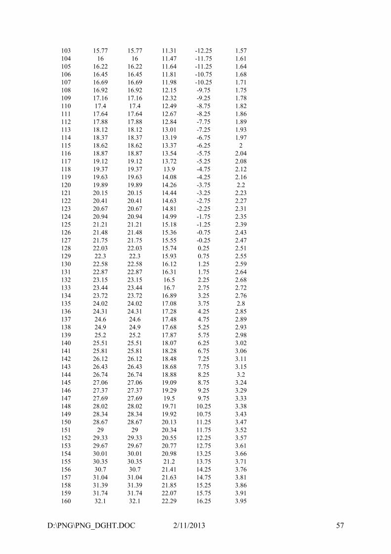
D:\PNG\PNG_DGHT.DOC 2/11/2013 57
103 15.77 15.77 11.31 -12.25 1.57
104 16 16 11.47 -11.75 1.61
105 16.22 16.22 11.64 -11.25 1.64
106 16.45 16.45 11.81 -10.75 1.68
107 16.69 16.69 11.98 -10.25 1.71
108 16.92 16.92 12.15 -9.75 1.75
109 17.16 17.16 12.32 -9.25 1.78
110 17.4 17.4 12.49 -8.75 1.82
111 17.64 17.64 12.67 -8.25 1.86
112 17.88 17.88 12.84 -7.75 1.89
113 18.12 18.12 13.01 -7.25 1.93
114 18.37 18.37 13.19 -6.75 1.97
115 18.62 18.62 13.37 -6.25 2
116 18.87 18.87 13.54 -5.75 2.04
117 19.12 19.12 13.72 -5.25 2.08
118 19.37 19.37 13.9 -4.75 2.12
119 19.63 19.63 14.08 -4.25 2.16
120 19.89 19.89 14.26 -3.75 2.2
121 20.15 20.15 14.44 -3.25 2.23
122 20.41 20.41 14.63 -2.75 2.27
123 20.67 20.67 14.81 -2.25 2.31
124 20.94 20.94 14.99 -1.75 2.35
125 21.21 21.21 15.18 -1.25 2.39
126 21.48 21.48 15.36 -0.75 2.43
127 21.75 21.75 15.55 -0.25 2.47
128 22.03 22.03 15.74 0.25 2.51
129 22.3 22.3 15.93 0.75 2.55
130 22.58 22.58 16.12 1.25 2.59
131 22.87 22.87 16.31 1.75 2.64
132 23.15 23.15 16.5 2.25 2.68
133 23.44 23.44 16.7 2.75 2.72
134 23.72 23.72 16.89 3.25 2.76
135 24.02 24.02 17.08 3.75 2.8
136 24.31 24.31 17.28 4.25 2.85
137 24.6 24.6 17.48 4.75 2.89
138 24.9 24.9 17.68 5.25 2.93
139 25.2 25.2 17.87 5.75 2.98
140 25.51 25.51 18.07 6.25 3.02
141 25.81 25.81 18.28 6.75 3.06
142 26.12 26.12 18.48 7.25 3.11
143 26.43 26.43 18.68 7.75 3.15
144 26.74 26.74 18.88 8.25 3.2
145 27.06 27.06 19.09 8.75 3.24
146 27.37 27.37 19.29 9.25 3.29
147 27.69 27.69 19.5 9.75 3.33
148 28.02 28.02 19.71 10.25 3.38
149 28.34 28.34 19.92 10.75 3.43
150 28.67 28.67 20.13 11.25 3.47
151 29 29 20.34 11.75 3.52
152 29.33 29.33 20.55 12.25 3.57
153 29.67 29.67 20.77 12.75 3.61
154 30.01 30.01 20.98 13.25 3.66
155 30.35 30.35 21.2 13.75 3.71
156 30.7 30.7 21.41 14.25 3.76
157 31.04 31.04 21.63 14.75 3.81
158 31.39 31.39 21.85 15.25 3.86
159 31.74 31.74 22.07 15.75 3.91
160 32.1 32.1 22.29 16.25 3.95

D:\PNG\PNG_DGHT.DOC 2/11/2013 58
161 32.46 32.46 22.51 16.75 4
162 32.82 32.82 22.73 17.25 4.05
163 33.18 33.18 22.96 17.75 4.11
164 33.55 33.55 23.18 18.25 4.16
165 33.92 33.92 23.41 18.75 4.21
166 34.29 34.29 23.64 19.25 4.26
167 34.67 34.67 23.87 19.75 4.31
168 35.05 35.05 24.1 20.25 4.36
169 35.43 35.43 24.33 20.75 4.42
170 35.81 35.81 24.56 21.25 4.47
171 36.2 36.2 24.79 21.75 4.52
172 36.59 36.59 25.03 22.25 4.57
173 36.99 36.99 25.26 22.75 4.63
174 37.39 37.39 25.5 23.25 4.68
175 37.79 37.79 25.74 23.75 4.74
176 38.19 38.19 25.98 24.25 4.79
177 38.6 38.6 26.22 24.75 4.85
178 39.01 39.01 26.46 25.25 4.9
179 39.42 39.42 26.7 25.75 4.96
180 39.84 39.84 26.95 26.25 5.01
181 40.26 40.26 27.19 26.75 5.07
182 40.68 40.68 27.44 27.25 5.13
183 41.11 41.11 27.69 27.75 5.18
184 41.54 41.54 27.94 28.25 5.24
185 41.97 41.97 28.19 28.75 5.3
186 42.41 42.41 28.44 29.25 5.36
187 42.85 42.85 28.69 29.75 5.42
188 43.3 43.3 28.94 30.25 5.48
189 43.75 43.75 29.2 30.75 5.54
190 44.2 44.2 29.46 31.25 5.6
191 44.65 44.65 29.71 31.75 5.66
192 45.11 45.11 29.97 32.25 5.72
193 45.57 45.57 30.23 32.75 5.78
194 46.04 46.04 30.5 33.25 5.84
195 46.51 46.51 30.76 33.75 5.9
196 46.99 46.99 31.02 34.25 5.96
197 47.46 47.46 31.29 34.75 6.02
198 47.94 47.94 31.56 35.25 6.09
199 48.43 48.43 31.82 35.75 6.15
200 48.92 48.92 32.09 36.25 6.21
201 49.41 49.41 32.37 36.75 6.28
202 49.91 49.91 32.64 37.25 6.34
203 50.41 50.41 32.91 37.75 6.41
204 50.92 50.92 33.19 38.25 6.47
205 51.43 51.43 33.46 38.75 6.54
206 51.94 51.94 33.74 39.25 6.6
207 52.46 52.46 34.02 39.75 6.67
208 52.98 52.98 34.3 40.25 6.74
209 53.5 53.5 34.58 40.75 6.81
210 54.04 54.04 34.87 41.25 6.87
211 54.57 54.57 35.15 41.75 6.94
212 55.11 55.11 35.44 42.25 7.01
213 55.65 55.65 35.73 42.75 7.08
214 56.2 56.2 36.02 43.25 7.15
215 56.75 56.75 36.31 43.75 7.22
216 57.31 57.31 36.6 44.25 7.29
217 57.87 57.87 36.89 44.75 7.36
218 58.43 58.43 37.19 45.25 7.43

D:\PNG\PNG_DGHT.DOC 2/11/2013 59
219 59 59 37.49 45.75 7.5
220 59.58 59.58 37.78 46.25 7.57
221 60.16 60.16 38.08 46.75 7.65
222 60.74 60.74 38.38 47.25 7.72
223 61.33 61.33 38.69 47.75 7.79
224 61.92 61.92 38.99 48.25 7.87
225 62.52 62.52 39.3 48.75 7.94
226 63.12 63.12 39.6 49.25 8.02
227 63.73 63.73 39.91 49.75 8.09
228 64.34 64.34 40.22 50.25 8.17
229 64.96 64.96 40.54 50.75 8.24
230 65.58 65.58 40.85 51.25 8.32
231 66.21 66.21 41.16 51.75 8.4
232 66.84 66.84 41.48 52.25 8.48
233 67.48 67.48 41.8 52.75 8.55
234 68.12 68.12 42.12 53.25 8.63
235 68.77 68.77 42.44 53.75 8.71
236 69.42 69.42 42.76 54.25 8.79
237 70.08 70.08 43.09 54.75 8.87
238 70.74 70.74 43.41 55.25 8.95
239 71.41 71.41 43.74 55.75 9.03
240 72.08 72.08 44.07 56.25 9.12
241 72.76 72.76 44.4 56.75 9.2
242 73.45 73.45 44.74 57.25 9.28
243 74.14 74.14 45.07 57.75 9.36
244 74.83 74.83 45.41 58.25 9.45
245 75.53 75.53 45.74 58.75 9.53
246 76.24 76.24 46.08 59.25 9.62
247 76.95 76.95 46.42 59.75 9.7
248 77.67 77.67 46.77 60.25 9.79
249 78.4 78.4 47.11 60.75 9.87
250 79.13 79.13 47.46 61.25 9.96
251 79.86 79.86 47.81 61.75 10.05
252 80.61 80.61 48.16 62.25 10.14
253 81.35 81.35 48.51 62.75 10.23
254 82.11 82.11 48.86 63.25 10.28
255 null null null null null