rapid identification of virtual cnc drives

Rapid Identification of

Virtual CNC Drives

by

Wilson Wai-Shing Wong

A thesis

presented to the University of Waterloo

in fulfillment of the

thesis requirement for the degree of

Master of Applied Science

in

Mechanical Engineering

Waterloo, Ontario, Canada, 2007

©Wilson Wai-Shing Wong, 2007

ii

AUTHOR'S DECLARATION FOR ELECTRONIC SUBMISSION OF A THESIS

I hereby declare that I am the sole author of this thesis. This is a true copy of the thesis,

including any required final revisions, as accepted by my examiners.

I understand that my thesis may be made electronically available to the public.

Wilson Wai-Shing Wong

iii

Abstract

Virtual manufacturing has gained considerable importance in the last decade. To obtain

reliable predictions in a virtual environment, the factors that influence the outcome of a

manufacturing operation need to be carefully modeled and integrated in a simulation

platform. The dynamic behavior of the Computer Numerical Control (CNC) system, which

has a profound influence on the final part geometry and tolerance integrity, is among these

factors. Classical CNC drive identification techniques are usually time consuming and need

to be performed by an engineer qualified in dynamics and control theory. These techniques

require the servo loop or the trajectory interpolator to be disconnected in order to inject the

necessary identification signals, causing downtime to the machine. Hence, these techniques

are usually not practical for constructing virtual models of existing CNC machine tools in a

manufacturing environment.

This thesis presents an alternative strategy for constructing virtual drive models with

minimal intervention and downtime to the machinery. The proposed technique, named “rapid

identification”, consists of executing a short G-code experiment and collecting input/output

data using the motion capture feature available on most CNC controllers. The data is then

processed to reverse engineer the equivalent tracking and disturbance transfer functions and

friction characteristics of the machine. It is shown that virtual drive models constructed this

way can be used to predict the real machine’s contouring performance for large class of drive

systems, controlled with different control techniques.

In the proposed scheme, the excitation is delivered by smoothly interpolated motion

commands. Hence, convergence of parameters to their true values is not guaranteed. When

the real system contains pole-zero cancellations, namely due to feedforward control action,

this also results in a loss of identifiability. In order to guarantee the stability of the identified

drive models, the pole locations are constrained with frequency and damping ratio limits.

Hence, the rapid identification task is cast as a constrained minimization problem.

Two solution strategies have been developed. In the first approach, Lagrange Multipliers

(LM) technique is applied, which yields successful estimation results. However,

iv

implementation of LM is computationally intensive and requires the use of a dedicated

symbolic solver. This limits the portability for industrial implementation. In the second

approach, a Genetic Algorithm (GA) search technique is developed, which is a more

practical but slightly approximate alternative. The GA allows parameter bounds to be

incorporated in a natural manner and converges to 2-3% vicinity of the LM solution in one-

tenth of the computation time. The GA solution can be easily ported to different computation

platforms.

Both LM and GA identification techniques were validated in simulations and

experiments conducted on virtual and real machine tool drives. It is shown that although the

parameters estimated using the rapid identification scheme do not always match their true

values, the key tracking and disturbance rejection characteristics of the drives are

successfully captured in the frequency range of the CNC motion commands. Therefore, the

drive models constructed with rapid identification can be used to predict the contouring

accuracy of real machine tools in a virtual process planning environment.

v

Acknowledgements

I would like to express my sincerest gratitude towards my advisor Dr. Kaan Erkorkmaz

for his invaluable support and encouragement throughout my graduate study. I consider it a

great privilege to work with him. Without his guidance, patience and wisdom this work

would not have been possible. I am indeed indebted to him for all that he has done for me.

I would also like to think my reading committee members, Drs. Michael Mayer and

William Melek who took the time to read my thesis and gave me advantageous

feedback.

Furthermore, I would like to thank my colleagues in the Precision Control Laboratory,

my friends, as well the faculty and staff, especially Robert Wagner, Andy Barber, and Steve

Hitchman, at the University of Waterloo – Department of Mechanical and Mechatronics

Engineering, who have made my experience at UW very enjoyable.

Finally, I would like to thank my beloved family for their unwavering support and

patience regarding my graduate study I dedicate this work to them.

vi

Table of Contents

Author’s Declaration ........................................................................................................ ii

Abstract ............................................................................................................................. iii

Acknowledgements .......................................................................................................... iii

Table of Contents ............................................................................................................. vi

List of Figures ................................................................................................................. viii

List of Tables ..................................................................................................................... x

Chapter 1

Introduction ....................................................................................................................... 1

1.1 Introduction ............................................................................................................... 1

Chapter 2

Literature Review ............................................................................................................. 4

2.1 Introduction ............................................................................................................... 4

2.2 Virtual CNC .............................................................................................................. 4

2.3 Modeling and Identification of Feed Drives ............................................................. 7

2.4 Evolutionary Computation ...................................................................................... 11

2.5 Summary ................................................................................................................. 13

Chapter 3

Rapid Identification Problem and Lagrange Multipliers Solution ............................ 14

3.1 Introduction ............................................................................................................. 14

3.2 Generalized Model for Closed Loop Axis Dynamics ............................................. 14

3.3 Constrained Parameter Identification using Lagrange Multipliers ......................... 18

3.4 Simulation and Experimental Results ..................................................................... 25

3.4.1 Simulation Results ............................................................................................ 26

3.4.2 Experimental Results ........................................................................................ 36

3.5 Conclusions ............................................................................................................. 39

Chapter 4 Constrained Parameter Estimation using a Genetic Algorithm .............. 40

4.1 Introduction ............................................................................................................. 40

vii

4.2 Genetic Algorithm Solution .................................................................................... 40

4.2.1 Initial (Parent) Population ................................................................................ 41

4.2.2 Crossover Operation ......................................................................................... 41

4.2.3 Mutation............................................................................................................ 43

4.2.4 Constraint Checking ......................................................................................... 44

4.2.5 Selection ........................................................................................................... 44

4.3 Simulation and Experimental Results ..................................................................... 47

4.3.1 Validation on a Virtual Machine Tool .............................................................. 48

4.3.2 Validation on a Ball Screw Drive ..................................................................... 50

4.3.3 Validation on a Machining Center .................................................................... 55

4.4 Conclusions ............................................................................................................. 59

Chapter 5

Conclusions ...................................................................................................................... 61

Chapter 6

References ........................................................................................................................ 63

Appendix A

Simulation and Experiment Results .............................................................................. 68

viii

List of Figures

Figure 2.1. Simulation of a machining path in CAD/CAM software. ...................................... 4

Figure 2.2. SimuCN® interface. ............................................................................................... 5

Figure 2.3. Overview of the Virtual CNC system. ................................................................... 6

Figure 2.4. Simplified drive dynamic model. ........................................................................... 7

Figure 2.5. General feed drive model in Virtual CNC. ............................................................. 8

Figure 2.6. Overview of rapid identification technique. ......................................................... 10

Figure 2.7. A Schematic of the Genetic Algorithm. ............................................................... 12

Figure 3.1. General representation of closed loop dynamics. ................................................. 15

Figure 3.2. Common control structures used in CNC drives. ................................................. 16

Figure 3.3. Allowable locations for (a) real, (b) complex poles. ............................................ 20

Figure 3.4. Identification trajectory captured in VCNC. ........................................................ 29

Figure 3.5. Estimated and actual tracking and disturbance frequency response functions

(FRF’s) for P-PI controlled servo system (simulation). .................................................. 30

Figure 3.6. Predicted and actual contouring of P-PI controlled servo system (simulation). .. 31

Figure 3.7. Predicted and actual contouring of P-PI controlled servo system (simulation). .. 32


(FRF’s) for PID controlled servo system (simulation). .................................................. 33

Figure 3.9. Predicted and actual contouring of PID controlled system (simulation). ............. 34


(FRF’s) for sliding mode controlled servo system (simulation). .................................... 35

Figure 3.11. Predicted and actual contouring performance of sliding mode controlled servo

system (simulation). ........................................................................................................ 36

Figure 3.12. Setup of one axis ballscrew system. ................................................................... 37

Figure 3.13. ZPETC + PPC + KF control scheme implemented on ball screw drive. ........... 38

Figure 3.14. Predicted and experimentally verified contouring performance for servo system

controlled with (a) pole placement, (b) zero phase error tracking control. ..................... 38

ix

Figure 4.1. Solution search space for GA identification. ........................................................ 41

Figure 4.2. Simulated binary crossover (SBX) operation. ...................................................... 42

Figure 4.3. Selection of best solution candidates. ................................................................... 45

Figure 4.4. Estimated parameters for PID controlled virtual drive. ........................................ 49

Figure 4.5. Predicted and actual tracking performance of virtual feed drive (simulation). .... 50

Figure 4.6. Estimated parameters for ZPETC + PPC + KF controlled ball screw drive

(experimental). ................................................................................................................ 51

Figure 4.7. Predicted and experimentally verified contouring performance of ball screw drive.

......................................................................................................................................... 54

Figure 4.8. Experimentally collected identification data from Heidenhain TNC 430 controller.

......................................................................................................................................... 58

Figure 4.9. Predicted and experimentally verified contouring performance of machining

center for a diamond toolpath (feedrate: 200 [mm/sec]). ............................................... 59


center for a circular toolpath (feedrate: 200 [mm/sec]). ................................................. 60

x

List of Tables

Table 3.1. Possible cases of constraint activation (cases 10, 12, 14, and 16 are infeasible). . 25

Table 3.2. Identification NC code. .......................................................................................... 27

Table 3.3.Actual and estimated closed loop parameters for P-PI controlled drive system. ... 30

Table 3.4. Actual and estimated closed loop parameters for PID controlled drive system. ... 33

Table 3.5. Actual and estimated closed loop parameters for SMC controlled drive system. . 35

Table 4.1. Actual and estimated parameters for PID controlled virtual drive. ....................... 49

Table 4.2. Actual and estimated parameters for ZPETC + PPC + KF controlled ball screw

drive. ............................................................................................................................... 52

Table 4.3. G-code used for generating low speed movements. .............................................. 56

Table 4.4. G-code used for generating high speed movements. ............................................. 56

Table 4.5. Estimated virtual drive parameters for Deckel Maho 80P hi-dyn machining center.

......................................................................................................................................... 58

1

Chapter 1

Introduction

1.1 Introduction

Virtual manufacturing has gained considerable importance in the last decade, with the

increasing availability of computational power which enables accurate simulation of complex

phenomena that govern manufacturing operations [1], [2]. The ability to predict, evaluate,

and optimize the performance of production machines and processes, without having to build

costly prototypes or run production trials, is highly appealing to both machine tool builders

and end users. The ultimate objective of virtual manufacturing is to achieve the shortest

possible cycle time and lowest cost, while maintaining the desired product quality from the

very first part onwards. The time, money, and engineering effort that could be saved through

sidestepping the prototyping and testing stages also promises shorter turnaround times for

putting new products on the market, in response to changing demands.

To obtain reliable predictions in a virtual environment, the factors that influence the

outcome of a manufacturing operation need to be carefully modeled and integrated into a

simulation platform. These factors typically originate from the process, the machine

dynamics, and the interaction between the two. Among factors pertaining to the machine tool,

the dynamic behavior of the Computer Numerical Control (CNC) system has a profound

influence on the final part geometry, as well as the tolerance integrity and surface quality.

When axis servo errors become excessive, the part geometry gets distorted and tolerances

may be violated. If the tool motion is not smooth, this would cause noticeable feed marks on

the machined part. In either case, the part may become unacceptable.

In order to predict the impact of the CNC system on the final part quality, a Virtual CNC

(VCNC) simulator was developed in [3]. The VCNC enables the contouring performance of

Chapter 1. Introduction 2

a real machine tool to be predicted and optimized in a virtual process planning environment.

However, its prediction accuracy relies strongly on the validity of feed drive models that are

identified from the actual machine. Standard identification tests are usually time consuming

and need to be performed by an engineer who is qualified in dynamics and control theory.

Sometimes, these experiments require the servo loop or the trajectory interpolator to be

disconnected, so special identification signals like sine or square waves, random noise, or

sine wave speeds can be injected into the servo system. When these factors are considered,

building even basic virtual models of CNC systems may require significant downtime to the

production machines, which is usually not practical in a manufacturing environment.

In this thesis, an alternative identification strategy is developed for constructing virtual

models of machine tool drives. The proposed technique, named “rapid identification”,

consists of executing a short G-code experiment and collecting input and output data using

the motion capture feature available on most CNC systems. The rapid identification test can

be conducted quickly, as if running a diagnostic routine, without any hardware or software

modification to the machine. The collected data is then processed with the intention of

reverse engineering the equivalent tracking and disturbance transfer functions of the closed

loop drive system, as well as the guideway friction. It is shown that a virtual drive model

constructed this way enables accurate prediction of the real machine’s contouring accuracy

for a variety of feed drive systems controlled with different control techniques.

The excitation input, in rapid identification, is delivered through motion commands

interpolated by trajectory generator. These signals are typically smooth up to the acceleration

level (i.e. 2C continuity) and lack the persistence of excitation to allow accurate estimation

of a large number of parameters. On the other hand, if the real servo system contains pole-

zero cancellations, which usually occur when feedforward action is employed in the

controller, this also results in incorrect estimation of the closed loop dynamics. Deviations

between the true and identified drive models are acceptable as long as the virtual model

captures the dynamics of the real drive system with sufficient closeness in the frequency

range of the CNC motion commands as observed in Section 3.4. In extreme cases, the non-

Chapter 1. Introduction 3

convergence of parameters can also result in the identification of critically stable or even

unstable virtual models, which have limited practical value. In order to avoid this problem,

bounds are imposed on the closed loop pole locations, which results in the identification

problem to assume the form of a constrained optimization problem.

Two solution strategies have been developed in this thesis. In the first approach,

Lagrange Multipliers (LM) technique is applied, which yields successful estimation results.

However, implementation of LM is found to be computationally intensive, and also requires

the use of a dedicated symbolic solver, like Matlab’s Symbolic Toolbox, to construct and

solve a system of nonlinear equations for each constraint activation case (i.e. Kuhn-Tucker

switching conditions [4]). These factors significantly limit the portability of the LM

technique for industrial implementation. As a more practical but slightly approximate

approach, a Genetic Algorithm search technique has also been developed. The GA’s ability

to constrain the search space allows the parameter bounds to be incorporated in a natural

manner. Computational speed of the GA has been streamlined by decoupling all a priori

calculations from the terms that need to be recomputed for each iterative cycle. It is shown

that the GA solution converges to 2-3% vicinity of the LM solution in one-tenth of the

computational time with a repeatable rate of 100%. The developed rapid identification

scheme has been verified in simulations and experiments conducted on virtual and real

machine tool drives. It is shown that the identified drive models can be successfully used for

predicting the contouring accuracy of real machine tools in a virtual process planning

environment.

4

Chapter 2

Literature Review

2.1 Introduction

This chapter presents a review of literature and industrial state-of-the-art in the areas of

virtual manufacturing, feed drive identification, and evolutionary programming. Section 2.2

introduces the concept of virtual manufacturing and the Virtual CNC framework. Various

techniques dedicated to the modeling and identification of feed drives are surveyed in

Section 0. Evolutionary programming, which is the basis of the Genetic Algorithm solution,

is introduced in Section 2.4. Conclusions for the chapter are presented in Section 2.5.

2.2 Virtual CNC

Many companies involved in manufacturing have started developing new technologies

and products that exploit modern computers’ ability to simulate manufacturing operations in

a virtual environment. CAD/CAM packages such as MasterCam® and ESPRIT® provide

toolpath visualization and analysis modules to help avoid potential collisions, which might

Figure 2.1. Simulation of a machining path in CAD/CAM software.

Chapter 2. Literature Review 5

occur during the machining process. A snapshot of such an interface is shown in Figure 2.1.

One disadvantage of these analysis tools is that they typically lack the dynamic information

about the machine or the manufacturing process, and provide only a geometric visualization

of what happens in the “ideal case”. Recently drive manufacturers like Omron™, Jtekt™,

and Schneider Electric™ have provided simulation software which allows the user to

simulate the dynamic behavior of a drive system, by providing NC code as the input. Such

software usually yields accurate predictions, since the drive parameters are known by the

manufacturer. An example application, SimuCN® developed by NUM™ CNC, is shown in

Figure 2.2. Other companies such as Siemens [5], Mori Seiki [6], and Ford Automotive [7]

have also been contributing the development of virtual manufacturing technologies, by

researching simulation systems that can predict and emulate the behavior of machining

centers and Computer Numerical Control (CNC) systems.

The overall objective of virtual manufacturing is to be able to combine the effect of

machine tool dynamics, manufacturing process, and the interaction between the two in a

common simulation platform. The Virtual CNC (VCNC) shown in Figure 2.3 was developed

Figure 2.2. SimuCN® interface.


at the University of British Columbia for this purpose; as a module to facilitate the simulation

of a real CNC system in a virtual environment. The Virtual CNC allows the performance of

machine tools to be optimized during design, development and end user stages [8], [9]. The

user can prototype a real CNC by selecting standard modules out of libraries of feed drive

models, control laws, trajectory generation algorithms, and feedback devices.

After the virtual CNC is configured, the contouring performance can be predicted and

optimized for different part programs. The VCNC can be used as a design and testing

platform by machine tool builders and controller developers [8], or as a process planning tool

by end users [10]. The prediction accuracy of the VCNC was verified in experiments

performed on real machinery, which matched the simulation results within less than 10%

error. Such prediction accuracy was only achievable after scrupulous modeling and

identification of the real machine’s feed drive dynamics, indicating the importance of having

a reliable model to obtain accurate predictions.

The structure of the VCNC is composed of three main functions: 1) The toolpath

interpolation; 2) Simulation of the drives’ response; 3) Performance evaluation. In the

toolpath interpolation, the trajectory commands are generated using a Cutter Location (CL)

CAD ModelCAD/CAM

System.....LOADTL/2FEDRAT/ 10000.00, MMPMRAPIDGOTO / 0.000, 0.000, 50.000

CL File Tool Path Geometry

sy

xPi

y

x

Pi+1

Pi

Pi+1

Pc

CL File Interpretation

ts

st

t

t

Displacement

Feedrate

Acceleration

Jerk

TrajectoryGeneration

r(t), r(t), r(t)

Feed Profiling

AxisCommands

Feed Drive Servo Dynamics

Axis MotionTracking Control

Feedback

Actual Axis Position

Axis Servo Loop

Tracking and Contour Error Estimation

Actual Tool Position with Servo Errors

s

s

Figure 2.3. Overview of the Virtual CNC system.


file which is obtained from a CAD/CAM package like Unigraphics® or CATIA®. The user

can select what type of feed profile (trapezoidal or S-curved velocity) will be used.

Simulation of the drive’s response considers the interaction between the open loop drive

dynamics and the servo controller. The user can configure a detailed drive model using

modules for ball screw (geared) or linear (direct driven) feed drives, available in a library.

The controller library contains a wide range of control laws ranging from simple P, PID, P-PI

cascade controllers to more complex techniques proposed in literature such as Pole-

Placement [11], Generalized Predictive [12], Adaptive Sliding Mode [13] and feedforward

[14], [15] control. Sensor noise, quantization, actuator saturation, backlash, and

computational delays can also be defined for each virtual CNC model. During performance

evaluation, important variables such as the contour error history, drive torque and current

signals are presented to the user in context of the commanded toolpath, which allows critical

regions to be easily identified. This enables corrective actions to be taken either by

modifying the part program or improving the CNC design. The Virtual CNC is currently a

module of CutPro machining process simulation software which is commercialized through

Manufacturing Automation Laboratories Inc., a UBC spin-off company.

2.3 Modeling and Identification of Feed Drives

The Virtual CNC is a promising tool towards achieving the overall objective of

simulating a complete digital factory in the virtual environment. However, the prediction

accuracy of the VCNC is strongly dependent on the correctness of the drive models that are

identified from real machinery. There has been extensive research in literature dedicated to

building models of feed drive systems, as reviewed in the following.

iTd-

Tu

ControlInput

Kt

MotorGain

Tm

Js+B1

Inertia andViscous Damping

s1 rg

ActualPosition

Disturbance Torque

Ka

CurrentAmplifier

xl

Figure 2.4. Simplified drive dynamic model.


One of the basic models which is widely used was proposed by Koren [16]. This model

considers only the linear rigid body dynamics, as shown in Figure 2.4. The current command

u injected into the current amplifier ( aK ) results in the armature current i , which is then

converted into actuation torque mT through the motor ( tK ). Part of the actuation torque is

consumed by disturbances ( dT ) originating from nonlinear guideway friction and possibly

the cutting process. The remaining torque actuates the drive system, which is represented by

an equivalent inertia J and viscous friction B reflected on the actuator. The motor angular

velocity ω is integrated to obtain angular position θ , which is then converted into linear axis

movement x through the gear ratio gr . Models have also been proposed that capture and

integrate the nonlinear effect of friction in the feed drive. Armstrong et al. [17] has presented

a very broad survey of the available techniques used to model and compensate friction in

servo systems. They have proposed a seven parameter model which adequately captures the

effect of pre-sliding displacement, static friction, and the full Streibeck curve describing how

the friction force changes with the relative sliding velocity between two surfaces in contact.

Later, Lee and Tomizuka [18] and Erkorkmaz and Altintas [19] have applied simpler

versions of this model to identify the friction dynamics in CNC drives. These models focus

primarily on the static, Coulomb, and viscous friction regimes.

iua Kt

MotorGain

s1 rg

Actual AxisPosition

Ka

CurrentAmplifier

xaJs+B1

Inertia andViscous Damping

Tc

-Tm

Disturb

ance D

ue to Cutting

forces

T+

Tf-+Ta

Non-Linear FrictionDynamics

Ta

uc

DACQuantization

with ZOH

uS

VoltageSaturation

xl

Backlash

Leadscrew & GearRatio

From Controller

ForceTransmissio nF (Cutting Force)

Tc

FrictionTorque, Tf

AngularVelocity, ω

+

+

D

input

output+ve-ve

xl

xa

Db2-

Db2

+0

Figure 2.5. General feed drive model in Virtual CNC.


The main disadvantage of rigid body type models is that they fail to capture the effect of

structural vibrations which becomes prevalent when high bandwidths are demanded in the

control law. To address these issues, Varanasi and Nayfeh [20] and Erkorkmaz and

Kamalzadeh [21] have worked on building Finite Element models and conducting frequency

response experiments to identify the torsional and axial vibrations of ball screw drives. The

backlash and motion loss in the nut interface have been identified by Kao et al. [22] and

Cuttino et al. [23], with models of varying complexity. The volumetric and thermal errors,

which influence the final tool positioning accuracy, were modeled by researchers at NIST in

[24]. Several of the listed models have successfully been incorporated into the general feed

drive template in the Virtual CNC shown in Figure 2.5.

Depending on circumstances, some of the dynamic factors listed above play a more

dominant role than the others in determining the final accuracy of a feed drive system. In

overall, experimental identification of models that capture the relevant dynamics is usually

time consuming and needs to be performed by an engineer who is competent in control

theory and sometimes metrology. The identification experiments may require the servo loop

or the interpolator to be disconnected, in order to inject particular excitation signals to the

drive system. When these factors are considered, building even basic virtual models of CNC

drives can result in considerable downtime to the actual production machines, which is not

always practical in a manufacturing environment.


To address these issues, a rapid identification strategy has been developed in this thesis,

which has been reported in [25], [26], and [27]. The rapid identification technique, shown in

Figure 2.6, consists of executing a short G-code experiment and collecting input and output

data using the “motion capture” feature available on most CNC systems. The data is

processed with the intention of reverse engineering the equivalent tracking and disturbance

transfer functions of the closed loop drive system, and the guideway friction. It is shown that

accurate prediction of the real machine’s contouring capability for a variety of feed drive

systems can be achieved through such virtual drive model.

One drawback of the rapid identification scheme is that the motion commands generated

by the interpolator are smooth, typically up to the acceleration level (i.e. 2C continuity), and

therefore lack the persistence of excitation to allow accurate estimation of all model

parameters using data captured for a short period of time. Furthermore, when feedforward

control is used to widen the effective tracking bandwidth, majority of the stable axis

Actual Machine Tool

Virtual DriveModel

CNCInterpolator

Feed DriveSystem

FeedbackMeasurement

ControlLaw

IdentificationNC Code

N10 G01X0.0 F12000N20 X0.258N30 X-0.790N40 X-2.992 ...

xref

xmeas

xact

xpredpred.error

--

+

d/dt

Gtrack(s)

Gdist(s) FrictionDisturbanceResponse

TrackingResponse

Figure 2.6. Overview of rapid identification technique.


dynamics are cancelled out by placing poles and zeros inside a trajectory pre-filter [14], [15].

This cancellation renders the identification of closed loop dynamics very difficult. In either

case, there is high likelihood that the identified parameters will not converge to their true

values. Such a deviation is normally acceptable, as long as the identified model captures the

dynamics of the real drive system with sufficient closeness in the frequency range of the

CNC motion commands. In extreme cases this non-convergence can also result in the

identification of critically stable or even unstable virtual drive models, which have very

limited practical value.

In order to guarantee stability of the identified model, bounds need to be imposed on the

closed loop pole locations. This results in the identification task to assume the form of a

constrained minimization problem, which has been solved using the Lagrange Multipliers

(LM) technique in [25], [26] and a Genetic Algorithm in [27]. LM theoretically yields the

best possible parameter estimates for the collected data, and this strategy was found to be

successful in identifying virtual drive parameters. However, it is a computationally lengthy

approach and requires the use of a specialized symbolic solver like Matlab’s Symbolic Math

Toolbox [28], which significantly limits its portability for industrial implementation. On the

other hand, the Genetic Algorithm (GA) is a slightly less exact approach but converges much

faster than the LM solution, and can be easily be ported to different platforms as it does not

require the use of a symbolic solver. The two approaches are explained in detail in Chapter 3

and Chapter 4.

2.4 Evolutionary Computation

Artificial Intelligence has been finding widespread use in solving complex engineering

problems which are difficult to solve using traditional algebraic or gradient based

optimization methods. There are three major areas of interest to engineers in the field of

artificial Intelligence; these are fuzzy logic, neural networks, and evolutionary programming

[29]. Fuzzy logic is used when the system does not have a direct relationship between the

inputs and outputs. Fuzzy logic is usually used for transferring existing expert knowledge

into automated decision making processes. Neural networks are used for mimicking


processes where the relationship between inputs and outputs are not exactly known, but can

be “learned” through observation, expert knowledge or pattern recognition. Genetic

Algorithms (GA’s) relate to an evolutionary programming technique which applies the

Principle of Natural Selection to find the best solution out of a large pool of candidates which

undergo several cycles of evolution. This concept was pioneered by Holland in his book in

1975 [30]; however it is Fogel who made this technique practical in the 1980’s, as an

alternative to classical approaches, by mimicking the evolutionary process in organ cells [31].

The ability to constrain the search space with desired bounds lends Genetic Algorithms to be

suitable for solving complex optimization problems in controller design and identification

which are constrained, nonlinear, multivariable, and typically non-convex [32].

A schematic of the GA is shown in Figure 2.7, which cycles through five main processes.

The first part of the cycle starts with a Parent Population of solution candidates. This

population is used to produce a new generation in the Crossover phase, which inherits

characteristics from the parent pairs. Randomness is introduced by perturbing the new

solutions in the Mutation phase. After ensuring compliance with the given constraints [32],

the solution candidates are evaluated for how well they minimize an overall objective. The

best solutions are then carried forward to spawn the next generation using the Selection

process. This cycle is repeated until the solution pool converges to the optimal result.

The main advantage of the Genetic Algorithm is the ease at which it can be adopted to

solve different kinds of problems. The designer only requires to supply the objective function

CROSSOVER

MUTATION INITIAL POPULATIONINITIAL (PARENT)

POPULATION

CONSTRAINT

SELECTION

Figure 2.7. A Schematic of the Genetic Algorithm.


and the constraints. Afterwards, the GA iteratively converges toward the optimal result. This

allows problems which are difficult to solve by algebra or conventional numerical techniques

to be efficiently handled. Although GA’s have been around since the 1980’s, it is with the

recent increase in the availability of computational power that they have become more

widespread. By restructuring the problem to streamline the computations and casting the

search in terms of the right parameters, Genetic Algorithms can provide solutions at a rate

which are comparable to deterministic calculations [33]. Problems such as airport traffic

control [34], shortest traveling distance between multiple points [35], operation planning of

NC processes [36], and AC motor modeling [37] have been successfully solved using GA’s.

Other applications in which GA’s have been applied are identifying the dynamics of

generators [38], [39], bearing stiffness and damping values in rotor assemblies [40], friction

models in precision linear stages [41], and robotic applications [42][43][44].

. In this thesis, the GA is used to identify the equivalent command following and

disturbance rejection properties and guideway friction in CNC machine tool drives, as

explained in Chapter 4.

2.5 Summary

This chapter has presented a survey of academic literature and industrial practice relevant

to virtual simulation of CNC systems, identification of feed drives, and the use of

evolutionary programming to solve complex engineering problems. It is shown that virtual

production simulations, as promising as they are, rely on the accuracy of the machine and

process models that are available. Hence, there is a strong need to identify dynamic models

of existing machine tools in a practical and reliable manner, while causing minimal

disruption to their operation. To address these issues, the concept of rapid identification has

been introduced, which will be further explained in the next two chapters.

14

Chapter 3

Rapid Identification Problem and Lagrange Multipliers Solution

3.1 Introduction

In this chapter, a mathematical framework is presented for solving the rapid identification

problem. In Section 3.2, a generalized model is developed which captures the key dynamics

of a large class of CNC drive systems. Based on this model, the constrained identification

problem is constructed and the solution is formulated in Section 3.3, using the Lagrange

Multipliers (LM) technique. Simulation and experimental results demonstrating the

effectiveness of the LM solution are presented in Section 3.4. The conclusions are presented

in Section 3.5.

3.2 Generalized Model for Closed Loop Axis Dynamics

In this section a dynamic model is developed which is applicable to a large class of CNC

drives. This model can be used to describe the overall closed loop behavior of ball screw or

linear drives, controlled with various feedback techniques such as P, PI, PD, PID, and P-PI

cascade control, with or without feedforward dynamic or friction compensation. The model

also considers the existence of nonlinear Coulomb friction, hence enabling the prediction of

quadrant glitches and tracking errors that arise from sudden changes in the friction field

during motion reversals. The main assumptions made in developing the model are: 1) Rigid

body motion is dominant (i.e. flexible modes are not excited); 2) Actuator saturations are

avoided; and 3) The effect of nonlinearities like torque ripples, backlash, and lead errors, are

minor in comparison to the servo errors that originate from the interaction between the

controller dynamics and the drive’s rigid body motion. These conditions are typically

realized on most feed drive systems.

Chapter 3. Rapid Identification Problem and Lagrange Multipliers Solution 15

Two of the most common control structures used in CNC drives are shown in Figure 3.2.

In Figure 3.2(a), the velocity loop is closed using proportional–integral (PI) control, and the

position loop is closed using proportional (P) control. In Figure 3.2(b), the position loop is

directly closed using a proportional-integral-derivative (PID) controller, which typically

results in motor torque commands. In both cases, feedforward compensation of axis

dynamics can be applied to widen the servo tracking bandwidth, in order to improve the

positioning accuracy. In the figure, J [kgm2] is the equivalent inertia and B [kgm2/sec] is

the viscous damping coefficient. u [V] is the torque command applied to the current

amplifier, K [Nm/V] is the product of the amplifier gain ( ampK [A/V]), motor torque

constant ( tK [Nm/A]), ball screw transmission gain ( gr [mm/rad]), and the gear ratio ( n ), if

there is one, between the motor and ball screw ( nrKKK gtamp= ). rx [mm] is the

commanded and x [mm] is the actual axis position. In both cases, the equivalent closed loop

dynamics can be represented in the form:

)(1

/)(1

1

)(

)(

3212

)(

3212

3210sd

saasas

JKsx

saasas

sabsbsb

sx

sGdist

r

sGtrack

⋅+++

−⋅+++

+++=

2

444 3444 21444 3444 21

(3.1)

Above )(sGtrack and )(sGdist are the equivalent tracking and disturbance transfer

functions. The most dominant source of nonlinear friction in feed drives is Coulomb and

static friction. A full model to describe the Stribeck curve requires extensive testing and

identification procedures to be carried out [17]. In this work, Coulomb friction is considered

Tracking TF

xr x

x-s2+a1s+a2+a3s-1

b0s2+b1s+b2+a3s-1

Scaled Disturbance TF Scaled Friction Model

s2+a1s+a2+a3s-1

1 ddt

d0 x>0

d1 x<0

Figure 3.1. General representation of closed loop dynamics.


as the main contributor to contouring and tracking errors during motion reversals. The

friction model is expressed in the form:

)NV()PV( xdxdd && ⋅+⋅= −+ (3.2)

where )PV(x& is a binary function which assumes a value of “1” when the axis velocity is

positive and “0” otherwise. )NV(x& takes a value of “1” when the axis velocity is negative

and “0” otherwise. +d and −d are the control signal equivalent values of Coulomb friction

for positive and negative directions of motion. Substituting the friction model in Eq. (3.2)

into the closed loop linear dynamics in Eq. (3.1) yields the general axis model shown in

Figure 3.1:

])NV()[PV()(]1[

)(]1[

103210

3212

dxdxsxs

absbsb

sxs

aasas

r ⋅+⋅−⋅+++=

⋅+++

2 && (3.3)

Kas2+Kvs+1 Kpxr x

d

PI Velocity Control LoopFeedforwardCompensation

FeedforwardCompensation

Frictiona) P-PI + Feedforward Control

P Position Control Loop

-

--

xuxr*

Kd +Kis

KJs+B

1s

xr

xr xd

Kas2+Kvs

Friction

b) PID + Feedforward Control

PID Position Control Loop

-

-

xuKd s + Kp + Ki

sK

Js+B1s

Figure 3.2. Common control structures used in CNC drives.


For the P-PI structure, the model parameters are obtained as:

⎪⎪⎪

⎭

⎪⎪⎪

⎬

⎫

==+

=

+==

=+

=+

=

−+ dJKdd

JKd

JKKKKK

b

JKKKKKK

bJ

KKKKb

JKKK

aJ

KKKKa

JKKB

a

ivdp

iavdpadp

ipipdd

102

10

321

,,)(

)(,

,)(

,

(3.4)

In the PID structure, the parameters become:

⎪⎪⎭

⎪⎪⎬

⎫

====+

=

===+

=

−+ dJKdd

JKd

JKK

abJ

KKKb

JKK

bJ

KKa

JKK

aJKKB

a

pvd

aipd

10221

0321

,,,)(

,,, (3.5)

It should be noted that the derived model in Eq. (3.3) allows the closed loop dynamics for

a large class of feed drive systems to be represented with only 8 parameters (3 poles, 3 zeros,

and 2 friction amplitudes). This model can also be used to capture the dominant dynamics of

drive systems controlled with more complex controllers such as state feedback and pole-

placement control. The time-dependent terms correspond to physically meaningful variables

such as commanded and actual axis position ( rx , x ), velocity ( rx& , x& ), acceleration ( rx&& , x&& ),

and integrated tracking error ( ∫ ττ−τt

r dxx0

)]()([ ). These profiles can be captured on the fly in

most CNC systems. If necessary, velocity and acceleration and integrated tracking error

profiles can be constructed through numerical differentiation or integration of discrete-time

position signals (i.e. )2/()(ˆ11 skkk Txxx −+ −=& , )2/()ˆˆ(ˆ

11 skkk Txxx −+ −= &&&& ,

∑ =−= k

m mmrski xxTe 1 ,, )( where sT : sampling period). The derived model can also capture

the response of simpler control structures, which may or may not contain feedforward,

integral, or derivative action. If feedforward friction compensation is used in the control law,

this results in lower values to be estimated for the remaining Coulomb friction. Finally, the


closed loop model is linear with respect to its parameters, allowing Least Squares type of

identification techniques to be applied [45].

3.3 Constrained Parameter Identification using Lagrange Multipliers

As shown in Figure 2.6 in Chapter 2, the rapid identification experiment is conducted by

executing a series of NC instructions comprised of short random linear movements, to deliver

as much excitation as possible to the drive system. The maximum feed and acceleration

values are set below the physical limits of the drives, in order to avoid actuator saturation.

The overall displacement range is selected such that the maximum feed can only be reached

when traveling from one end of the motion range to the other. The commanded displacement

between consecutive NC blocks is generally too short to reach the desired maximum feedrate,

which enables the performance of the drive to be observed for a wide range of feeds within

the machine’s working envelope. The execution of multiple back and forth movements at

different velocities allow for the effect of Coulomb friction, which brings amplitude

dependence into the drive model, to be clearly observed. In order to deliver the excitation in

as high frequency range as possible, smooth acceleration profiling (i.e. “S-curve”

functionality) should be disabled in the interpolator, if possible. This results in trapezoidal

and triangular velocity transitions, which provide higher frequency content, as opposed to

parabolic velocity transitions.

The axis position commands and encoder measurements ( krx , and kx ) are collected

while running the identification NC code. The data collection is carried out at the control

loop period sT for a total of N samples. The objective is to find the parameters ( 1a , 2a , 3a ,

0b , 1b , 2b , 0d , 1d ) for the dynamic model in Eq. (3.3) such that the discrepancy between

measured ( kx ) and predicted ( kx̂ ) axis movements is minimized in a least squares sense:

∑=

−=N

kkk xxf

1

2]ˆ[21 Minimize :Objective

(3.6)


The motion commands generated by the interpolator are relatively smooth and generally

lack the persistence of excitation for all estimated parameters to converge to their true values,

even though only rigid body motion is considered. This is not a major problem, as long as the

identified drive model captures the key dynamics of the real system within the frequency

range of the CNC motion commands. However, incorrect estimation of the drive dynamics

may also result in unstable or poorly damped pole locations, which have limited practical

value for conducting virtual manufacturing simulations. In order to avoid this problem and

guarantee stability of the identified drive models, bounds need to be imposed on the

frequency and damping ratio values of the closed loop poles. The characteristic polynomial

in Eq. (3.3) and its pole locations are:

23,21

31

2232

21

3

1 ,

)()2)((

ζ−ω±ζω−=−=

−=ω+ζω++=+++ ∏ =

nn

k knn

jppp

pssspsasasas

(3.7)

As the damping ratio becomes large ( 1>>ζ ), the third closed loop pole starts

approaching zero (i.e. −→ 03p ), which is undesirable. In order to guarantee the necessary

stability margins, the closed loop pole frequencies need to be constrained with lower bounds

and the damping ratio needs to be constrained with lower and upper bounds, resulting in the

below statement of identification constraints:

⎭⎬⎫

≤≥≥≥

:,::,:

:sConstraintmax4min3

min,2min1

ζζζζωω

hhhpph nn

(3.8)

where 0min >p , 0min. >ωn , and 0minmax >ζ>ζ . Assuming that 1max >ζ , the

allowable pole locations are shown in Figure 3.3. In the following, the identification problem

is solved as a constrained minimization problem using Lagrange Multipliers technique with

Kuhn-Tucker switching conditions [4], in order to handle the inequality constraints.


Assuming that the commanded position ( krx , ), velocity ( krx ,& ), acceleration ( krx ,&& ),

measured velocity ( kx& ) and acceleration ( kx&& ), and integrated tracking error

( ∑ =−= k

m mmrsi xxTe 1 , )( ) are available at the kth sample, the axis position can be predicted

by taking the inverse Laplace transform of Eq. (3.3): −+ δ⋅−δ⋅−β+β+β+α−α−α= )NV()PV(ˆ ,2,1,021, kkkrkrkrkkkiik xxxxxxxex &&&&&&&& (3.9)

The model parameters, normalized with respect to 2a (i.e. coefficient for axis position)

are obtained as:

⎪⎭

⎪⎬

⎫

========

−+ /,//,/,//,/,/1

2120

220211202

2321122

adadabababaaaaa i

δδβββααα

(3.10)

The identification problem is solved to determine the vector of normalized model

parameters ( θ ). Clustering the axis position measurements into an output vector: Y and

defining the regressor matrix Φ ,

Im

Re2−pmin

p1 p2 p3

ImAllowableRegion

(b)(a)

Re

Figure 3.3. Allowable locations for (a) real, (b) complex poles.


TNxxx ][ 21 K=Y

⎥⎥⎥⎥

⎦

⎤

⎢⎢⎢⎢

⎣

⎡

−−−−

−−−−−−−−

=

)NV()PV(

)NV()PV()NV()PV(

,,,,

222,2,2,222,

111,1,1,111,

NNNrNrNrNNNi

rrri

rrri

xxxxxxxe

xxxxxxxexxxxxxxe

&&&&&&&&

MMMMMMMM

&&&&&&&&

&&&&&&&&

Φ

Ti ][ 21021

−+ δδβββααα=θ

(3.11)

the objective function in Eq. (3.6) is re-expressed as:

)()(21 Minimize :Objective ΦθYΦθY −−= Tf (3.12)

The inequality constraints in Eq. (3.8) are transformed into equality constraints using the

slacking variables 1σ , 2σ , 3σ , ℜ∈σ4 :

⎪⎪⎭

⎪⎪⎬

⎫

=−+−=⇒≥+−=−−=⇒≥−=−−=⇒≥−

=−−=⇒≥−

00:00:

00:00:

:sConstraint

24max4max4

23min3min3

22min,2min,2

21min1min1

σζζζζσζζζζσωωωω

σ

hhhhhh

pphpph

nnnn

(3.13)

Considering Eq. (3.7) and (3.10), the first three optimization variables ( iα , 1α , 2α ) are

related to the constraint variables ( p , nω , ζ ) as:

nnnn

n

nn

ni

papp

aa

pp

aa

ζω+ω==α

ζω+ω

ζω+==α

ζω+ω

ω==α

211 ,

22 ,

2 22

222

112

2

2

3

(3.14)

The differential relationship between these variables can be constructed as by taking the

total differential of the expressions in Eq. (3.14):


2

2

222222

222

222

111

2

1

)2(/2/)(2/2

/)(2/)(24122

:where

/////////

ζωωωζωωζ

ωωωζωζωζωζω

ζω

ζω

ζαωααζαωααζαωαα

ααα

pppppp

pp

dddp

dddp

ppp

ddd

n

nnnn

nnnnn

nn

nn

n

n

iniii

+

⎥⎥⎥

⎦

⎤

⎢⎢⎢

⎣

⎡

−+−−−−++−−

−

=

⎥⎥⎥

⎦

⎤

⎢⎢⎢

⎣

⎡⋅=

⎥⎥⎥

⎦

⎤

⎢⎢⎢

⎣

⎡⋅

⎥⎥⎥

⎦

⎤

⎢⎢⎢

⎣

⎡

∂∂∂∂∂∂∂∂∂∂∂∂∂∂∂∂∂∂

=⎥⎥⎥

⎦

⎤

⎢⎢⎢

⎣

⎡

G

G

(3.15)

The inverse gradient can then be obtained by inverting the matrix G :

)2/()2(2

)2(2

)(2

22/)2(2/2/)2(

: where, //////

///

22

222

32

32

1

2

11

2

1

21

21

21

ζωωζω

ωζωζωωζω

ωωζζωζωωζω

ωωω

ααα

ααα

αζαζαζαωαωαω

ααα

ζω

ppp

ppppppp

pp

ddd

dddppp

dddp

nnn

nnnn

n

nn

nnnn

nnn

ii

i

nnin

i

n

++−

⎥⎥⎥⎥⎥

⎦

⎤

⎢⎢⎢⎢⎢

⎣

⎡

−−−−

+−−

−−−−

=

⎥⎥⎥

⎦

⎤

⎢⎢⎢

⎣

⎡⋅=

⎥⎥⎥

⎦

⎤

⎢⎢⎢

⎣

⎡⋅

⎥⎥⎥

⎦

⎤

⎢⎢⎢

⎣

⎡

∂∂∂∂∂∂∂∂∂∂∂∂

∂∂∂∂∂∂=

⎥⎥⎥

⎦

⎤

⎢⎢⎢

⎣

⎡

−

−

G

G

(3.16)

The constrained optimization problem is solved by constructing the augmented objective

function ),,,,,,,,(' 43214321 σσσσλλλλθf and setting its partial derivatives with respect to

the optimization variables (θ ), Lagrange multipliers ( 4321 ,,, λλλλ ) and slacking variables

( 4321 ,,, σσσσ ) to zero:

⎩⎨⎧

=∂∂=∂∂=∂∂=∂∂=∂∂=∂∂=∂∂=∂∂=∂∂

−+−+−−+

−−+−−+−−=

0/' ,0/' ,0/' ,0/'0/' ,0/' ,0/' ,0/' ,/'

:Solution

)()(

)()()()(21'

4321

4321

24max4

23min3

22min,2

21min1

4433

2211

σσσσλλλλ

σζζλσζζλ

σωωλσλ

λλ

λλ

fffffffff

ppf

hh

h

nn

hf

T

0θ

ΦθYΦθY

444 3444 2144 344 21

444 3444 2144 344 21444 3444 21

(3.17)


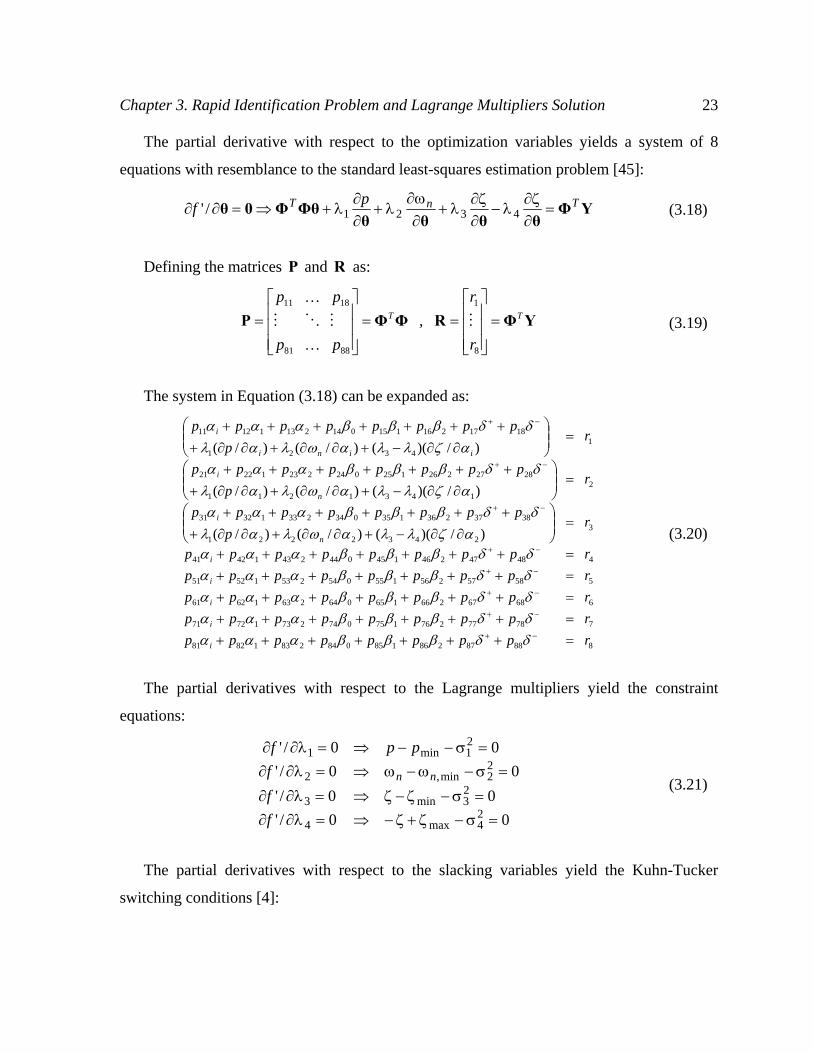
The partial derivative with respect to the optimization variables yields a system of 8

equations with resemblance to the standard least-squares estimation problem [45]:

YΦθθθθ

ΦθΦ0θ TnT pf =∂ζ∂

λ−∂ζ∂

λ+∂ω∂

λ+∂∂

λ+⇒=∂∂ 4321/'

(3.18)

Defining the matrices P and R as:

YΦRΦΦP TT

r

r

pp

pp=

⎥⎥⎥

⎦

⎤

⎢⎢⎢

⎣

⎡==

⎥⎥⎥

⎦

⎤

⎢⎢⎢

⎣

⎡=

8

1

8881

1811

, M

K

MOM

K

(3.19)

The system in Equation (3.18) can be expanded as:

8888728618508428318281

7787727617507427317271

6686726616506426316261

5585725615505425315251

4484724614504424314241

32432221

383723613503423313231

21431211

282722612502422312221

14321

181721611501421311211

)/)(()/()/(

)/)(()/()/(

)/)(()/()/(

rpppppppprpppppppprpppppppprpppppppprpppppppp

rp

pppppppp

rp

pppppppp

rp

pppppppp

i

i

i

i

i

n

i

n

i

iini

i

=+++++++=+++++++=+++++++=+++++++=+++++++

=⎟⎟⎠

⎞⎜⎜⎝

⎛

∂∂−+∂∂+∂∂++++++++

=⎟⎟⎠

⎞⎜⎜⎝

⎛

∂∂−+∂∂+∂∂++++++++

=⎟⎟⎠

⎞⎜⎜⎝

⎛

∂∂−+∂∂+∂∂++++++++

−+

−+

−+

−+

−+

−+

−+

−+

δδβββαααδδβββαααδδβββαααδδβββαααδδβββααα

αζλλαωλαλδδβββααα



(3.20)

The partial derivatives with respect to the Lagrange multipliers yield the constraint

equations:

00/'00/'

00/'00/'

24max4

23min3

22min,2

21min1

=σ−ζ+ζ−⇒=λ∂∂=σ−ζ−ζ⇒=λ∂∂

=σ−ω−ω⇒=λ∂∂=σ−−⇒=λ∂∂

fff

ppf

nn

(3.21)

The partial derivatives with respect to the slacking variables yield the Kuhn-Tucker

switching conditions [4]:


020/'020/'020/'

020/'

444

333

222

111

=σλ−⇒=σ∂∂=σλ−⇒=σ∂∂=σλ−⇒=σ∂∂=σλ−⇒=σ∂∂

ffff

(3.22)

These equations imply that the ith constraint is either active ( 0=σi , equality state), or

inactive ( 0=λ i , inequality state) [4]. Considering that there are four constraints, this leads

to 1624 = possible constraint activation scenarios, which have been shown in Table 3.1.

Among these, Cases 10, 12, 14, and 16 are infeasible, since they correspond to maxζ=ζ and

minζ=ζ holding at the same time, which is not possible if minmax ζ>ζ . Case 1 corresponds

to the unconstrained solution of Eq. (3.12), which is the result of the standard Least Squares

technique [45]. If the solution for this case violates the bounds in Eq. (3.8), then the

remaining 11 cases need to be evaluated one by one. For each feasible case, the system in

Eqs. (3.20)-(3.21) is reconstructed and solved by substituting in the known values of

Lagrange multipliers and slacking variables from Table 3.1, the partial derivatives ( ip α∂∂ / ,

1/ α∂∂p , 2/ α∂∂p , in α∂ω∂ / , 1/ α∂ω∂ n , 2/ α∂ω∂ n , iα∂ζ∂ / , 1/ α∂ζ∂ , 2/ α∂ζ∂ ) from Eq.

(3.16), and replacing the iα , 1α , 2α terms with their expressions in terms of p , nω , and ζ

from Eq. (3.14). Each nonlinear equation system is solved using Matlab’s Symbolic Math

Toolbox [28], resulting in a solution (or in some cases, multiple solutions) for p , nω , ζ , 0β ,

1β , 2β , +δ , −δ , the unknown Lagrange multipliers and the slacking variables. The

normalized denominator parameters iα , 1α , 2α , are computed using Eq. (3.14). Each

solution is checked for constraint feasibility (Eq. (3.13)) and feasible solutions are evaluated

for how well they minimize the objective function (Eq. (3.12)). The feasible solution that

yields the lowest value for the objective is selected as the optimal parameter set ( 1a , 2a , 3a ,

0b , 1b , 2b , 0d , 1d ) for the dynamic model in Eq.(3.3).


3.4 Simulation and Experimental Results

The effectiveness of the proposed identification strategy has been verified in simulations

and experimental case studies conducted on virtual and actual feed drives. Since virtual axis

dynamics are already known, the simulations allow a comparison between the true and

identified drive parameters. The experiments were conducted to validate practical

effectiveness of the rapid identification strategy.

The NC code used in the tests is shown in Table 3.2, which consists of 200 random linear

movements commanded within a range of ±10 [mm] with a maximum feedrate of 200

[mm/sec]. Due to the short travel distance between consecutive position commands, this

velocity is not reached. Instead, the drive’s response is observed for a wide range of

Table 3.1. Possible cases of constraint activation (cases 10, 12, 14, and 16 are infeasible).

Case 1λ 1σ 2λ 2σ 3λ 3σ 4λ 4σ 1 0 0 0 0

2 0 0 0 0

3 0 0 0 0

4 0 0 0 0

5 0 0 0 0

6 0 0 0 0

7 0 0 0 0

8 0 0 0 0

9 0 0 0 0

10 0 0 0 0

11 0 0 0 0

12 0 0 0 0

13 0 0 0 0

14 0 0 0 0

15 0 0 0 0

16 0 0 0 0


velocities, as intended. The maximum acceleration and deceleration values for the

interpolator were set to 2000 [mm/sec2], which correspond to the limits of the drive system.

The S-curve functionality in the interpolator was disabled, which produced trapezoidal

velocity profiles with sharper motion transients. This was done to improve the parameter

convergence. The data was collected at a sampling period of sT =1 [msec] for a duration of

22 [sec]. A sample data set captured for a window of 1 [sec] is shown in Figure 3.4. The

signals comprise of commanded, measured, and modeled (identified) position profiles.

In applying the Lagrange Multipliers solution, the pole location bounds were selected as

minp = min,nω =6.28 [rad/sec] (1 [Hz]), minζ =0.2 [ ], and maxζ =2.0 [ ]. The LM solution was

implemented in Matlab on a Pentium IV computer. The use of the Symbolic Math Toolbox

brought significant overhead to the computation of the solution, which sometimes took up to

15-20 minutes when all constraint activation scenarios needed to be checked. Nevertheless,

the models identified with the LM technique were quite successful in replicating the real

drive systems’ dynamic response, as demonstrated in the following subsections.

3.4.1 Simulation Results

In the simulations, a virtual model of a Fadal VMC 2216 machining center was used,

which was constructed through careful identification of the rigid body dynamics, nonlinear

guideway friction, amplifier current limits, nut backlash, DAC quantization, and encoder

measurement noise This model had been thoroughly verified in tracking and contouring

experiments conducted on the real machine using different control schemes in earlier work

[8]. The simulations were conducted considering different control structures to be

implemented on the machine, such as P-PI cascade, PID, and adaptive sliding mode control.


Table 3.2. Identification NC code. N0000 G00 X0.000 F12000 N0010 G01 X 0.258 N0020 G01 X-0.790 N0030 G01 X-2.992 N0040 G01 X-8.099 N0050 G01 X-1.327 N0060 G01 X 4.185 N0070 G01 X-7.681 N0080 G01 X-8.438 N0090 G01 X-2.615 N0100 G01 X-9.327 N0110 G01 X-6.157 N0120 G01 X-0.573 N0130 G01 X-7.102 N0140 G01 X 4.357 N0150 G01 X 3.234 N0160 G01 X-1.363 N0170 G01 X-1.079 N0180 G01 X 0.167 N0190 G01 X 0.562 N0200 G01 X 1.458 N0210 G01 X-2.784 N0220 G01 X-3.270 N0230 G01 X-6.535 N0240 G01 X-8.278 N0250 G01 X-2.133 N0260 G01 X 6.087 N0270 G01 X-9.778 N0280 G01 X-5.338 N0290 G01 X 8.677 N0300 G01 X-5.464 N0310 G01 X 5.719 N0320 G01 X-1.785 N0330 G01 X-7.612 N0340 G01 X 2.687 N0350 G01 X 7.248 N0360 G01 X-6.835 N0370 G01 X 2.024 N0380 G01 X-7.648 ...

... N1630 G01 X-8.131 N1640 G01 X-5.721 N1650 G01 X 1.918 N1660 G01 X-8.511 N1670 G01 X 8.689 N1680 G01 X-0.193 N1690 G01 X-0.128 N1700 G01 X-4.498 N1710 G01 X 1.432 N1720 G01 X 7.033 N1730 G01 X 3.820 N1740 G01 X 6.886 N1750 G01 X-5.564 N1760 G01 X 7.172 N1770 G01 X-2.652 N1780 G01 X 0.551 N1790 G01 X 4.521 N1800 G01 X-9.637 N1810 G01 X-1.713 N1820 G01 X 8.878 N1830 G01 X9.849 N1840 G01 X-5.730 N1850 G01 X-4.483 N1860 G01 X 0.362 N1870 G01 X 5.308 N1880 G01 X-7.907 N1890 G01 X-5.381 N1900 G01 X-3.796 N1910 G01 X 2.959 N1920 G01 X-3.515 N1930 G01 X-1.919 N1940 G01 X 4.187 N1950 G01 X 9.234 N1960 G01 X 3.739 N1970 G01 X 6.345 N1980 G01 X-6.731 N1990 G01 X 9.038 N2000 G01 X-2.641 N2010 G01 X 0.000


P-PI Cascade Controlled System

The rapid identification strategy was first evaluated on a P-PI cascade controlled drive

system. The identification converged to the unconstrained solution without any of the

stability constraints (Eq.(3.21)) becoming active. The true and estimated closed loop

parameters are summarized in Table 3.3. A comparison between the true and estimated

tracking and disturbance frequency response functions (FRF’s) is presented in Figure 3.5. As

can be noted in the table, there is discrepancy between the true and estimated pole locations.

Although the slowest pole ( 3p ) at 4.68 [Hz] is captured with reasonable closeness at 4.88

[Hz] in x and y axes, the complex conjugate poles ( 1p and 2p ) which actually have a

frequency of 36.26 [Hz] are estimated as a pair of real poles at 368.80 and 47.84 [Hz] for x,

and 436.91 and 45.52 [Hz] for y axes. The zero ( 3z ) at 21.88 and 21.90 [Hz] in the x and y

axes is closely estimated at 23 and 22.81 [Hz] respectively. In addition, there is around 16.9×

and 18.4× mismatch between the estimated and true friction parameters ( 0d and 1d ) in x and

y axes.


Considering the FRF’s shown in Figure 3.5 (a) and (b) it is seen that the identified

transfer functions are able to represent the tracking characteristics of the x and y axes

accurately up to a frequency range of 30 [Hz], which is reasonably wide for tracking most

CNC motion commands.

0

0.1

0

10

0

200

0 0.1 0.2 0.3 0.4 0.5 0.6 0.7 0.8 0.9 1.0

0

5000

Sample Data Collected for Identification

Trac

king

Err

or [m

m]

Pos

ition

[mm

]V

eloc

ity[m

m/s

ec]

Time [sec]

Acc

eler

atio

n[m

m/s

ec2 ]

Axis CommandMeasured ResponseModeled Response

Figure 3.4. Identification trajectory captured in VCNC.


Table 3.3.Actual and estimated closed loop parameters for P-PI controlled drive system.

X Axis Y Axis Actual Estimated Actual Estimated

Para

met

ers

1a 372.76 2648.46 372.76 3061.862a 62009.83 776813.58 61999.31 878064.603a 1527104.87 21349028.29 1527104.86 24070716.710b 0 1.08 0 1.191b 0 -415.03 0 -472.932b 11106.33 65194.67 11095.82 75718.610d 441 7210 409 75231d -302 -5277 -388 -7160

Poles and Zeros

Frequency [Hz]

Damping [ ]

Frequency[Hz]

Damping[ ]

Frequency[Hz]

Damping[ ]

Frequency [Hz]

Damping [ ]

Pole

s 1p 36.26 0.75 368.80 1.00 36.26 0.75 436.91 1.002p 36.26 0.75 47.84 1.00 36.26 0.75 45.52 1.003p 4.68 1.00 4.88 1.00 4.68 1.00 4.88 1.00

Zero

s 1z − − 58.91 -0.72 − − 59.74 -0.722z − − 58.91 -0.72 − − 59.74 -0.723z 21.88 1.00 23.00 1.00 21.90 1.00 22.81 1.00

100 101Frequency [Hz]

102

-200-150-100

-50

-250

10-4

10-5

10-6

10-7

0Actual

Estimated(dashed)

Actual

Estimated(dashed)

(a) X Axis Tracking Transfer Function

(c) X Axis Disturbance FRF

(b) Y Axis Tracking Transfer Function

(d) Y Axis Disturbance FRF

Pha

se[d

eg]

Mag

nitu

de[m

m/m

m]

Mag

nitu

de[m

m/V

]

101

100

10-1


102


102 100 101Frequency [Hz]

102

-100-50

050

-150

100

Pha

se[d

eg]

ActualEstimated(dashed)

ActualEstimated(dashed)

Figure 3.5. Estimated and actual tracking and disturbance frequency response

functions (FRF’s) for P-PI controlled servo system (simulation).


In addition, considering the real and estimated disturbance transfer functions (Figure

3.5 (c) and (d)), it can be seen that there is close agreement in the phase shift up to 10 [Hz]

and a D.C. amplitude difference of 13.9× for x and 15.7× for y axes, which compensates for

the discrepancy between true and estimated friction parameters to a large extent. In overall, it

can be said that the estimated transfer functions are successful in capturing the key dynamic

characteristics required to predict the tracking and contouring performance of the actual

drives with reasonable closeness. The actual and identified axis dynamics have been

compared in tracking circular and diamond shaped toolpaths at 200 [mm/sec] feed with 2000

[mm/sec2] trapezoidal acceleration transients. The comparison results are shown in Figure

3.6 and Figure 3.7, which are seen to be in close agreement.

Tracking Errors Contour Error [mm]

X A

xis

[mm

]

0 0.1 0.2 0.3 0.4 0.5 0.6 0.7Time [sec]

05

10Actual

Predicted(dashed)0

0.51.01.5

0 0.1 0.2 0.3 0.4 0.5 0.6 0.7

Y A

xis

[mm

]

Time [sec]

05

10

0 5 10 15 200

5

10

15

20

25

30

35

40Toolpath

X Axis [mm]

Toolpath (Zoomed View)

X Axis [mm]

Y A

xis

[mm

]

Y A

xis

[mm

]

19 20 2118

19

20

21 CommandedToolpath

ActualToolpath

PredictedToolpath(dashed)

Figure 3.6. Predicted and actual contouring of P-PI controlled servo system

(simulation).


PID Controlled System

The second simulation study was conducted for a PID controlled drive system, which

does not have an inner velocity control loop. The actual and estimated drive parameters are

summarized in Table 3.4.

As seen from the table, there is close match in this case between the actual and identified

pole and zero locations. This is verified by the consistency in the actual and estimated

frequency response functions (Figure 3.8), both for tracking and disturbance. The tracking

transfer functions are in close agreement up to 30 [Hz]. The disturbance transfer functions

appear to be in agreement up to 80 [Hz]. When averaged, there is 15 [%] discrepancy

between the actual and estimated friction parameters ( 0d and 1d ).

Tracking Errors Contour Error [mm]

X A

xis

[mm

]

Time [sec]

Y A

xis

[mm

]

Time [sec]

0 5 10 15 200

5

10

15

20

25

30

35

40Toolpath

X Axis [mm]


X Axis [mm]

Y A

xis

[mm

]

Y A

xis

[mm

]

19 20 2118

19

20

21

CommandedToolpath

ActualToolpath Predicted

Toolpath(dashed)

0 0.2 0.4 0.6 0.8 1.0

0 0.2 0.4 0.6 0.8 1.0

05

05

00.10.20.3

ActualPredicted(dashed)

Figure 3.7. Predicted and actual contouring of P-PI controlled servo system (simulation).


Table 3.4. Actual and estimated closed loop parameters for PID controlled drive system.


Para

met

ers

1a 192.65 214.13 178.75 123.02

2a 44356.23 60040.19 41031.98 40099.88

3a 316830.21 685295.65 293085.57 146558.19

0b 0 -0.35 0 -0.08

1b 190.10 203.86 175.85 123.16

2b 44356.23 60043.78 41031.98 40089.20

0d 441 620 409 478

1d -302 -280 -388 -428Poles

and Zeros Frequency

[Hz] Damping

[ ] Frequency

[Hz] Damping

[ ] Frequency

[Hz] Damping

[ ] Frequency

[Hz] Damping

[ ]

Pole

s 1p 33.00 0.45 38.21 0.42 31.74 0.43 31.69 0.302p 33.00 0.45 38.21 0.42 31.74 0.43 31.69 0.303p 1.17 1.00 1.89 1.00 1.17 1.00 0.59 1.00

Zero

s 1z − − 129.50 -1.00 − − 270.83 -1.002z 35.96 1.00 32.88 1.00 35.96 1.00 42.98 1.003z 1.17 1.00 1.89 1.00 1.17 1.00 0.59 1.00


102

-100-50

050

-150

10-4

10-5

10-6

Actual

Estimated (dashed)

Actual

Estimated (dashed)

Estimated (dashed)





Pha

se[d

eg]

Mag

nitu

de[m

m/m

m]

Mag

nitu

de[m

m/V

]

101

100

10-1


102



102-200

0100

Pha

se[d

eg]

Actual

Estimated(dashed)

-100

Actual


(FRF’s) for PID controlled servo system (simulation).


The circular and diamond contouring results for the actual and estimated transfer

functions are shown in Figure 3.9, which are also in close agreement.

Adaptive Sliding Mode Controlled System

The third control structure which was evaluated is adaptive sliding mode control. When

adaptation is conducted only for the unknown disturbance, the control law assumes a PID-

like structure with feedforward velocity and acceleration terms [13]. The true and estimated

drive parameters are summarized in Table 3.5. Due to the existence of feedforward control

action, there is full pole-zero cancellation in both axes, resulting in a tracking transfer

function equal to unity with zero phase shift in the ideal case. This makes the accurate

identification of drive parameters very difficult. It is seen that the identified poles and zeros

do not match their true values. However, the near-cancellation effect can be observed

between poles at 7.04 and 93.76 [Hz] and zeros at 7.05 and 101.62 [Hz] in the x axis, and

poles at 7.86 and 108.50 [Hz] and zeros at 7.87 and 116.02 [Hz] in the y axis, yielding

reasonably flat tracking transfer functions up to 50 [Hz] range, as seen in Figure 3.10(a) and

(b). There is 5.8× and 5.1× inconsistency between actual and estimated friction model

parameters, in x and y axes, which is compensated by the 4.0× and 3.9× D.C. gain difference

in the real and estimated disturbance transfer functions (Figure 3.10 (c) and (d)), which are in

close phase agreement up to 10 [Hz].

0 0.1 0.2 0.3 0.4 0.5 0.6 0.7 0 0.2 0.4 0.6 0.8 1.0

(a) Circular Toolpath (b) Diamond ToolpathTracking Errors

Actual

Predicted (dashed)

Contour Error

Tracking ErrorsX

Axi

s [u

m]

Y A

xis

[um

]C

onto

ur

Err

or [u

m]

Time [sec]

Contour Error

Time [sec]

050

050

020406080

05

101520

050

050

Figure 3.9. Predicted and actual contouring of PID controlled system (simulation).


Table 3.5. Actual and estimated closed loop parameters for SMC controlled drive system.


Para

met

ers

1a 390.10 566.95 493.09 449.092a 57029.44 370137.94 87925.67 484496.303a 3801962.50 15346572.85 5861711.35 22962987.980b 1.00 0.85 1.00 0.871b 390.10 574.83 493.09 455.362b 57029.44 370142.25 87925.67 484500.130d 441 2367 409 20231d -302 -1858 -388 -2016

Poles and Zeros

Frequency[Hz]

Damping [ ]

Frequency[Hz]

Damping[ ]

Frequency[Hz]

Damping[ ]

Frequency [Hz]

Damping [ ]

Pole

s 1p 31.83 1.00 93.76 0.44 31.83 1.00 108.50 0.292p 21.94 0.69 93.76 0.44 27.25 0.86 108.50 0.293p 21.94 0.69 7.04 1.00 27.25 0.86 7.86 1.00

Zero

s 1z 31.83 1.00 101.62 0.50 31.83 1.00 116.02 0.322z 21.94 0.69 101.62 0.50 27.25 0.86 116.02 0.323z 21.94 0.69 7.05 1.00 27.25 0.86 7.87 1.00


102

-10-505

-15

10-4

10-5

10-6

10-7

Actual

Estimated(dashed)

Actual

Estimated(dashed)





Pha

se[d

eg]

Mag

nitu

de[m

m/m

m]

Mag

nitu

de[m

m/V

]

101

100

10-1


102



102

050

-50

100

Pha

se[d

eg]

Actual

Estimated(dashed)

Estimated(dashed)

-100-150

Actual

Figure 3.10. Estimated and actual tracking and disturbance frequency response

functions (FRF’s) for sliding mode controlled servo system (simulation).


The contouring results obtained with the actual and estimated drive models for the two

toolpaths are shown in Figure 3.11, which are again in agreement.

The simulation results validate the proof of concept for the proposed rapid identification

strategy. They show that theoretically it is possible to construct virtual models of existing

feed drives, using data captured during a short G-code experiment. Although the identified

models may not exactly have the same parameters as the actual drive system, they are still

successful in predicting the tracking and contouring accuracies of CNC machine tools for

different part programs.

3.4.2 Experimental Results

Following successful concept validation in simulation results, the rapid identification

technique was tested experimentally on a ball screw drive, to demonstrate its practical

effectiveness. The ball screw drive setup, controlled with a dSPACE motion controller, is

shown in Figure 3.12. Position measurements were obtained from the encoder mounted on

the motor, which provides a resolution equivalent to 1.25 [um] of table motion. Due to the

availability of only a single drive, the x and y axis trajectories were tested separately and the

results were synchronized by overlapping the command trajectories, which enabled the

estimation of equivalent contour error profiles.

010

010

0 0.1 0.2 0.3 0.4 0.5 0.6 0.7

51015

0 0.2 0.4 0.6 0.8 1.0

(a) Circular Toolpath (b) Diamond Toolpath

0

010

010

51015

0

Tracking Errors

ActualPredicted (dashed)

Contour Error

Tracking Errors

X A

xis

[um

]Y

Axi

s [u

m]

Con

tour

E

rror

[um

]

Time [sec]

Contour Error

Time [sec] Figure 3.11. Predicted and actual contouring performance of sliding mode controlled

servo system (simulation).


Two control cases have been considered: In the first case, the control loop is closed using

a Pole Placement Controller (PPC) [11] with a Kalman Filter (KF) [46] for disturbance

observation and cancellation. In the second case, a Zero Phase Error Tracking Controller

(ZPETC) [14] is added to the scheme, to widen the tracking bandwidth with feedforward

control action. The implemented control scheme is shown in Figure 3.13. The ZPETC

improves the tracking accuracy by widening the overall command following bandwidth. In

order to achieve this, it cancels out all of the poles and stable (or well damped) zeros of the

closed loop system achieved with the pole-placement controller. Considering Figure 3.13, the

discrete-time transfer function between the filtered position commands )(* zxr and the final

axis position )(zx can be expressed as,

)()()(

)()()(

)()(

* zAzBzB

zAzBzG

zxzx

r

−+===

(3.23)

In the numerator, )(zB+ contains all of the stable and well-damped, and )(zB− contains

the unstable or poorly damped zeros. The expression for the ZPETC is given as [14],

2

1*

)]1()[()()(

)()()(

−+

−−==

BzBzBzA

zxzxzG

r

rZPETC

(3.24)

Figure 3.12. Setup of one axis ballscrew system.


It can be shown that this results in an overall tracking transfer function of

2

1

)]1([)()()()(

)()(

−

−−− ⋅=⋅=

BzBzBzGzG

zxzx

ZPETCr

(3.25)

which has zero phase shift at all frequencies, and a gain very close to one for a wide

frequency range. After conducting the rapid identification, the axis models were verified by

running the circular toolpath in Figure 3.6 at 100 [mm/sec] feed with 600 [mm/sec2]

trapezoidal acceleration transients. The actual and predicted tracking and contour error

profiles are shown in Figure 3.14, which are in close agreement for both the low bandwidth

(PPC + KF) and high bandwidth (PPC + KF + ZPETC) controllers, thus demonstrating the

practicality and effectiveness of the proposed identification scheme.

ZPETCPole

PlacementControl

KalmanFilter

Ball ScrewDrive

xr u u, xd

Feedback

Disturbance

d ̂DisturbanceEstimation &Cancellation

++

-PositionTrajectory

xr *

Figure 3.13. ZPETC + PPC + KF control scheme implemented on ball screw drive.

00.01

(a) PPC + KF (b) ZPETC + PPC + KFTracking Errors Tracking Errors

X A

xis

[mm

]Y

Axi

s [m

m]

Con

tour

E

rror [

um]

Time [sec]

Contour Error

Time [sec]

00.01

0 0.2 0.4 0.6 0.8 1.0 1.2 1.4 1.605

1015

00.51.0

00.51.0

0 0.2 0.4 0.6 0.8 1.0 1.2 1.4 1.605

1015

Actual Predicted(dashed)

Contour Error

Figure 3.14. Predicted and experimentally verified contouring performance for servo

system controlled with (a) pole placement, (b) zero phase error tracking control.


3.5 Conclusions

This chapter has provided a basic mathematical framework for the rapid identification

strategy. It has presented a solution which utilizes Lagrange Multipliers for solving the

constrained identification problem. This guarantees the stability of identified drive models,

regardless of the lack of excitation in the command signals, or presence of pole-zero

cancellations in the drive dynamics. The practicality and effectiveness of the proposed

identification scheme has been demonstrated in simulation and experimental results, in which

the tracking and contouring accuracy of a real drive system could be successfully predicted in

a virtual process planning environment. One major downfall of the Lagrange Multipliers

technique was found to be its mathematical complexity, which required the use of a

dedicated symbolic math solver in order to handle different constraint activation cases. This

resulted in a computationally lengthy solution, which sometimes took up to half an hour on a

Pentium IV Personal Computer. The dependence on a symbolic solver also limits the

portability of the LM solution for industrial implementation. In the next chapter, these issues

have been addressed by developing an alternative strategy to solve the constrained

identification problem more efficiently, using a Genetic Algorithm.

40

Chapter 4

Constrained Parameter Estimation using a Genetic Algorithm

4.1 Introduction

In this chapter, a Genetic Algorithm (GA) approach is developed for solving the

constrained identification problem defined in earlier Chapter 3. The structure of the GA is

explained in detail in Section 4.2. This is followed by simulation and experimental results

that validate the practicality and effectiveness of the GA identification scheme. The

conclusions are presented in Section 4.4.

4.2 Genetic Algorithm Solution

The structure of the proposed Genetic Algorithm (GA) is shown in Figure 2.7. It is

similar to the one proposed by Fogel et al. [33]. The first part of the cycle starts with a Parent

Population of solution candidates. This population is used to produce a new generation in the

Crossover phase, which inherits its characteristics from the parent pairs. Randomness is

introduced by perturbing the new solutions in the Mutation phase. After ensuring compliance

with the stability constraints [32], the solution candidates are evaluated for how well they

minimize the objective in Eq. (3.12). The best solutions are carried forward to spawn the next

generation using the Selection process. This cycle is repeated until the solution pool

converges to an optimal set of parameters which best replicate the observed feed drive

response. In setting up the GA identification, the solution search is conducted directly in

terms of the closed loop pole frequency ( pn ,ω ) and damping )(ζ values, as shown in Figure

4.1. Adopting this strategy simplifies the incorporation of stability constraints expressed in

Eq. (3.8). The upper bounds for pole frequencies ( maxmax, , pnω ) are set to half of the

Chapter 4. Constrained Parameter Estimation using a Genetic Algorithm 41

sampling frequency (i.e. Nyquist frequency) used in the data collection process. The

following notation is adopted in describing the GA identification framework:

⎩⎨⎧

=Number Candidate :Number Generation :

where),,( , it

pti

ti

tin

ti

ti ζωυυ

(4.1)

It should be noted that the GA identification technique can easily be generalized to

handle more complex problems with a larger number of parameter constraints. In this case,

each constrained parameter would be introduced as an additional bounded variable, resulting

in the search space to assume the form of a hyperprism. In the following, phases of the GA

identification scheme are explained in detail.

4.2.1 Initial (Parent) Population

The initial population is generated with a uniform distribution within the highlighted

search space in Figure 4.1. After the first cycle is complete, the new parent generation is

determined through a selection process applied on the mutated solution candidates from the

earlier generation.

4.2.2 Crossover Operation

The crossover operation spawns the next generation of candidates by combining pairs

from the current generation. It has a smoothening effect on the solution pool, which

facilitates convergence. Every solution candidate ( tiυ ) is randomly matched with another

p

pmin

pmax

ζ

ζmin

ζmax

ωn

ωn,min

ωn,max

SearchSpace

Figure 4.1. Solution search space for GA identification.


candidate ( tjυ ). These pairs are then used to produce two new candidates in the next

generation: 1+tiυ and 1+t

jυ . Since the solution candidates are made up of real numbers, the

crossover operation needs to be conducted in the domain of real numbers instead of binary.

To achieve this, the Simulated Binary Crossover (SBX [47]) operation was adopted with a

slight modification which prevents the divergence of the new generation away from the

parents. The process of SBX is shown in Figure 4.2. The implemented SBX has the

following mathematical expression [47],

⎩⎨⎧

≥−<

=

++

−=

−+

+=

+

+

++

5.0,)]1(2[5.0,)2(

:where

21

21 ,

21

21

1/1

1/1

11

rrrr

n

n

tj

ti

tj

tj

ti

ti

α

αααα υυυυυυ

(4.2)

The specific case use in this thesis is n = 2,

⎩⎨⎧

≥−<

=

++

−=

−+

+= ++

5.0,)]1(2[5.0,)2(

:where

21

21 ,

21

21

3/1

3/1

11

rrrr

tj

ti

tj

tj

ti

ti

α

αααα υυυυυυ

(4.3)

A) B) 0 0.5 1

Parent 1

Parent 2

Offspring 1

Offspring 2

Random Weight (r)

Sol

utio

n C

andi

date

Figure 4.2. Simulated binary crossover (SBX) operation.


Above, r is a random weighting factor with a uniform distribution between zero and one,

which determines the closeness of the offspring to one of the parents. Possible outcomes of

the SBX operation are illustrated in Figure 4.2.

4.2.3 Mutation

Mutation is used to randomly perturb the candidates in the new generation. This helps

prevent the Genetic Algorithm from converging to local minima. Each candidate is perturbed

in the form:

)1,0(]'[ 11iii

ti

ti NRη+= ++ υυ (4.4)

Above, )1,0(iN is a random number generated with a normal distribution which has zero

mean and unit variance. This variable is computed separately for each candidate. iR is a

scaling factor defined as,

⎩⎨⎧

>−≤−

=+

+

0)1,0(,3/)(0)1,0(,3/)(

1max

min1

iti

iti

i NN

Rυυυυ

(4.5)

Considering that 99.73% of the values generated by )1,0(iN will be in the range of -3 to

+3 (i.e. three standard deviations), the scaling factor iR maps these outcomes such that the

perturbed solutions span the search space in Figure 4.1 bounded by the corners points

),,( minminminmin pζωυ and ),,( maxmaxmaxmax pζωυ . The iη term represents a momentum

step size, which is employed in evolutionary programming to facilitate larger perturbation in

initial cycles. As iterations continue, iη converges to a stationary random sequence around

“1”. Its mathematical expression is given as [31],

tt

NN iti

2/1' , 2/1 :where

))1,0()1,0('exp(

==

+=

ττ

ττη

(4.6)


Above, )1,0(tN is generated from a normally distributed random sequence,

independently from )1,0(iN . )1,0(tN is updated only once for each generation. Essentially,

)1,0(iN represents individual mutations which can affect each candidate separately while

)1,0(tN represents an overall mutation affecting the whole generation. τ and 'τ ensure that

the step size is different for each iteration.

4.2.4 Constraint Checking

Each candidate is checked for compliance with the constraints. If any value of nω , ζ , or

p is outside the valid search range, it is replaced by the closest bound:

⎪⎭

⎪⎬

⎫

=⇒>=⇒<=⇒>=⇒<=⇒>=⇒<

maxmaxminmin

maxmaxminmin

max.,max.,min.,min.,

]'[]'[if,]'[]'[if]'[]'[if,]'[]'[if]'[]'[if,]'[]'[if

pppppppp ti

ti

ti

ti

ti

ti

ti

ti

nt

innt

innt

innt

in

ζζζζζζζζωωωωωωωω

(4.7)

4.2.5 Selection

Selection of successful candidates is carried out using a hybrid approach which combines

Top Percent and Random Tournament techniques, as shown in Figure 4.3. Top Percent

ensures that solutions which yield the lowest value for the objective in Eq. (3.12) are

included in the crossover process. Random Tournament, on the other hand, arbitrarily

matches pairs out of the mutated pool and selects the superior candidate out of each pair.

This approach may lead to the same candidate being chosen more than once, as seen with

4'υ for example in Figure 4.3.

During implementation of the GA, numerical evaluation of the cost function was found to

bring the largest computational load. Naming N as the number of collected data samples,

computing the objective function using the form in Eq. (3.12) would require 239 +N

multiplications, 169 +N additions, and 1 division. Typically N is larger than 1000 and in

our experimental results 8192=N . In order to avoid this computational bottleneck,


calculation of the objective function was realized in a more efficient manner as explained in

the following paragraphs.

The parameter vector θ in Eq. (3.11) can be separated into two parts as:

TTTT

iTT

][][ 2121021

21

θθθθθ

== −+

444 3444 2143421δδβββααα

(4.8)

Given the pole frequency and damping values for a particular solution candidate

),,( ,ti

ti

tin

ti pζωυ , the normalized denominator parameters T

i ][ 211 ααα=θ can be

determined using Eq. (3.14). The remaining parameters T][ 2102−+ δδβββ=θ can

then be uniquely calculated by constructing a Least Squares sub-problem [45], assuming that

the inverse for 22 ΦΦ T exists. Hence,

( )1121

2221122 )( θΦYΦΦΦθθΦYθΦ −=⇒−= − TT (4.9)

Using this idea, and modifying the notation to represent each solution candidate as

)( ti

ti υμ where,

Ti

ti

ti ]1[)( 21 ααα=υμ (4.10)

,,,,,,

,,

... ......

TopPercentSelection

RandomTournamentSelection

MutatedSolutions

SurvivingSolutions

,,

,,,

,,

,,

Figure 4.3. Selection of best solution candidates.


the normalized drive parameters can be solved in the form:

⎪⎪⎪⎪

⎭

⎪⎪⎪⎪

⎬

⎫

⎥⎥⎥

⎦

⎤

⎢⎢⎢

⎣

⎡

⎥⎥⎥

⎦

⎤

⎢⎢⎢

⎣

⎡=

⎥⎥⎥

⎦

⎤

⎢⎢⎢

⎣

⎡

⎥⎥⎥

⎦

⎤

⎢⎢⎢

⎣

⎡=⎥

⎦

⎤⎢⎣

⎡−

=

−

−

838281

4342411

8884

4844

8

41

8884

48443

* and

* where, **

0

ppp

ppp

pp

pp

r

r

pp

ppti

ti

MMM

L

MOM

L

M

L

MOM

L

P

RμPRI

θ

(4.11)

It should be noted that the matrix terms ijp and kr are directly the individual entries of

P and R matrices defined in Eq. (3.19). The value of the objective function (i.e. fitness) for

each candidate can then be evaluated by expanding Eq. (3.12) using Eqs. (4.10) and (4.11),

which results in:

⎪⎪⎪

⎭

⎪⎪⎪

⎬

⎫

=

⎥⎦

⎤⎢⎣

⎡−

−=⎥⎦

⎤⎢⎣

⎡−⎥

⎦

⎤⎢⎣

⎡

−=

++=

×

××

YYΓ

PRΙ

RΒPRΙ

PPΙ

RΑ

ΓΒμΑμμυ

T

TT

T

ti

ti

Tti

tif

11

314

3

344

, **

02 ,

**0

**0

where

)]([21)(

(4.12)

Above, matrices Α , B , and Γ depend solely on the experimental data and are computed

only once prior to running the Genetic Algorithm. Given ),,( ,ti

ti

tin

ti pζωυ for a solution

candidate, evaluation of the objective function using Eq. (4.12) requires only 32

multiplications, 22 additions and 1 division, hence reducing the computational load by 2-3

orders of magnitude. It should be noted that a similar reduction can also be obtained in more

complex problems with a larger number of constrained variables. This step, which improves

the numerical efficiency, was crucial in realizing a practically viable Genetic Algorithm for

solving the constrained identification problem. This numerical simplification is also one of

the contributions in this thesis.


4.3 Simulation and Experimental Results

The Genetic Algorithm identification technique was validated in simulations and

experiments conducted on virtual and real feed drive systems. Simulations were conducted

on a virtual machine tool model to verify the parameter convergence and servo error

prediction capability. Experiments were conducted on a ball screw drive and a 5-axis

machining center, to demonstrate the practicality and effectiveness of the GA. Where

applicable, the GA has been compared to the LM technique described in Chapter 3.

The GA was configured to have a population size of 4000 candidates in each generation.

The parameter search ranges were set as min,nω = minp =0.2 [Hz], max,nω = maxp =500 or 800

[Hz] (depending on the sampling frequency), minζ =0.2, and maxζ =2.0. The crossover rate is

0.5 and the mutation rate is 0.05. The selection operation was carried out by choosing the

best 5 solutions (i.e. 0.125%) using the Top Percent approach, and the remaining using the

Random Tournament approach, as explained in Section 4.2.5. The GA was implemented in

Matlab on a Pentium IV computer. The implementation did not require the use of any

specialized toolboxes and was written in a manner that could be directly ported into C++ or

any other programming language. The Lagrange Multipliers solution was also implemented

in Matlab on the same PC platform, but required the use of the Symbolic Math Toolbox, as

mentioned in Chapter 2, to handle cases where the unconstrained solution of Eq. (3.12)

violated the parameter bounds in Eq. (3.8).

The LM solution represents the best theoretical estimate that could be obtained with the

collected data and given parameter constraints. When all constraint activation cases need to

be checked, the solution takes around 15-20 minutes to compute. On the other hand, the

Genetic Algorithm was observed to converge within 2-3% closeness of the LM solution in

about 2-3 minutes, making the GA a more practical alternative to the LM approach, even if it

is slightly less exact. Sample results are presented in the following.


4.3.1 Validation on a Virtual Machine Tool

In the first example, the Genetic Algorithm is compared to the Lagrange Multipliers (LM)

solution in simulation results obtained using the virtual machine tool model (Fadal VMC

2216) reported in Section 3.4.1. The drive’s axes were controlled using PID controllers tuned

to provide a bandwidth of 57 [Hz]. The rapid identification data generated by running the G-

code in Table 3.2 was used.

The identification results obtained with the two schemes are shown in Figure 4.4 and

Table 4.1. Figure 4.4 shows the convergence of GA parameter estimates to the LM solution.

Table 4.1 presents the actual and estimated values of the search variables, model parameters,

and tracking transfer function zeros. Considering Figure 4.4, it can be seen that in about 300

iterations, the Genetic Algorithm converges closely to the LM solution. The actual solutions

are captured at 500 iterations with a repeatability rate of 100%. All the test cases result are

documented in Appendix A.


0246

p [H

z]

0.350.400.450.50

0 50 100 150 200 250 300

36384042

Iteration

Genetic Algorithm (solid)Lagrange Multipliers Solution (dashed)

Figure 4.4. Estimated parameters for PID controlled virtual drive.

Table 4.1. Actual and estimated parameters for PID controlled virtual drive.

Search variables Actual Lagrange Multipliers

Estimate Genetic Algorithm

Estimate nω [Hz] 33 38.21 38.20

ζ [ ] 0.45 0.42 0.42 p [Hz] 1.17 1.89 1.94

Model Parameters Actual Lagrange Multipliers


Estimate 1a 192.65 214.13 214.41

2a 44356.23 60040.19 60072.73

3a 316830.21 685295.65 703594.29

0b 0 -0.35 -0.34

1b 190.1 203.86 203.74

2b 44356.23 60043.78 60076.41

0d 441 620 627

1d -302 -280 -277Zero

Locations Actual Lagrange Multipliers Estimate

Genetic Algorithm Estimate

1z [Hz] -35.96 127.32 129.58

2z [Hz] -1.17 -32.72 -32.87

3z [Hz] - -1.89 -1.95


As shown in Table 4.1, the natural frequency and damping ratio are estimated in a

consistent manner between both solutions ( LMn,ω =38.21, GAn,ω =38.20 [Hz] and

LMζ = GAζ =0.42), and the estimates are reasonably close to their true values ( Actualn,ω =33

[Hz], Actualζ =0.45). The estimates for the real pole are also consistent among each other

( LMp =1.89, GAp =1.94 [Hz]), but slightly different from the actual pole location

( Actualp =1.17 [Hz]). Considering that the real pole is cancelled by a zero in all cases

( Actualz ,2 = −1.17, LMz ,3 = −1.89, GAz ,3 = −1.95 [Hz]), this pole does not have any effect on

the command following properties but it influences the response of axis position to

disturbances, as can be inferred from the block diagram in Figure 3.1. The GA identified

model was validated in a tracking simulation using a trajectory of ±20 [mm] of forward and

backward motion commanded at a feedrate of 70.71 [mm/sec] with acceleration transients of

424.26 [mm/sec2]. The simulation result is shown in Figure 4.5, in which the tracking error,

using the reference trajectory, predicted with the GA identified model is generally within 10-

15% closeness of the actual tracking error.

4.3.2 Validation on a Ball Screw Drive

20100

-10-20

50

0

-50

5

0

-5

Posi

tion

[mm

]Tr

acki

ngEr

ror [

um]

Pred

ictio

nD

iscr

epan

cy[u

m]

0 0.2 0.4 0.6Time [sec]

0.8 1.0

GA Identified Model (solid)

Actual Tracking (dashed)

Figure 4.5. Predicted and actual tracking performance of virtual feed drive (simulation).


In the second example, the GA is tested on the ball screw drive controlled with the

ZPETC + PPC + KF scheme, explained in Section 3.4.2. As mentioned earlier, in this control

configuration accurate identification of the closed loop dynamics is very difficult, due to the

pole-zero cancellations that take place between the feedback loop and the ZPETC. The

parameter convergence obtained using experimental identification data is shown in Figure

4.6. As can be seen, the GA estimates converge closely to the LM solution in less than 50

iterations. The actual discrete-time controller design parameters and model estimates

obtained with GA and LM techniques are shown in Table 4.2. The control system was

designed at a sampling period of sT = 1 [msec] and the closed loop poles were placed at

2,1p =0.86846+j0.11762 in the z-domain, corresponding to a natural frequency of

Actualn,ω =30 [Hz] and a damping ratio of Actualζ =0.7. These poles are cancelled out by the

zeros of the ZPETC at 4,3z =0.86846+j0.11762, and replaced by two deadbeat delay terms

4,3p =0. The closed loop zero at 1z =-0.99937, which is very close to -1, is not directly

cancelled out but its phase lag is removed by incorporating another zero at 2z = −1.0006

3456

0.1

0.2

0.3

76788082 Genetic Algorithm (solid)

Lagrange Multipliers Solution (dashed)

p [H

z]

0 50 100 150 200 250 300Iteration

Figure 4.6. Estimated parameters for ZPETC + PPC + KF controlled ball screw drive (experimental).


through spectral factorization (i.e. 1/−0.99937= −1.0006) and adding an additional delay term

5p =0 to make the ZPETC causal.

It was shown in [48] that additional closed loop poles contributed by the Kalman filter do

not affect the tracking transfer function, as they get cancelled out by collocated zeros. Hence,

their effect is ignored, which simplifies the ZPETC design and analysis. During parameter

identification and model validation the command trajectory was shifted forward in time by 2

samples, which is the preview horizon of the designed ZPETC [14]. One shift accounts for

the pole excess and the other for the number of unstable zeros, in the closed loop system.

Table 4.2. Actual and estimated parameters for ZPETC + PPC + KF controlled ball screw drive.

Actual Parameters (discrete-time system)

Search Variables

Lagrange Multipliers Estimate

Genetic Algorithm Estimate

Sampling Period nω [Hz] 77.83 77.30

sT = 0.001 [sec] ζ [ ] 0.203 0.202 PPC + KF (closed loop) p [Hz] 4.36 4.39

Poles 2,1p =0.86846+j0.11762 Model

ParametersLagrange Multipliers


Estimate ( nω =30 [Hz], ζ =0.7)

Zeros 1z =-0.99937 1a 225.94 223.76ZPETC (feedforward filter) 2a 244579.87 241310.90Poles 3a 6551189.40 6510957.51

5,4,3p = 0 (3 delays) 0b 0.75 0.76Zeros 1b 240.24 238.13

2z = -1.0006

4,3z = 0.86846 + j0.11762

2b 244452.20 241460.26

0d 1032.57 1024.55Overall Transfer Function 1d -996.03 -987.61

Poles Zero Locations

Lagrange Multipliers Estimate

Genetic Algorithm Estimate 3,2,1p′ = 0 (3 delays)

Zeros 1z [Hz] -4.37 -4.39

2,1z′ = -1.0006, -0.99937 3,2z ω =89.76 [Hz], ζ =0.26 ω =88.65 [Hz], ζ =0.26


Considering the LM and GA estimates, it is seen that the natural frequency, damping

ratio, and real poles are estimated consistently between the two techniques: LMn,ω =77.83,

GAn,ω =77.30, LMp =4.36, GAp =4.39 [Hz], LMζ =0.203, GAζ =0.202. The identified natural

frequency and damping ratio, however, are very different from their actual closed loop values

of Actualn,ω =30 [Hz] and Actualζ =0.7. Furthermore, the damping estimate is very close to its

minimum acceptable limit minζ =0.2. The identified zero locations are also close to the pole

estimates LMz ,1 = −4.37, GAz ,1 = −4.39, LMz ,3,2ω =89.76, GAz ,3,2

ω =88.65 [Hz], LMz ,3,2 ζ =0.26,

GAz ,3,2ζ =0.26, thus emulating the effect of “cancelled dynamics” observed in the real system.

In this example, the dominant closed loop poles were estimated at significantly different

locations than their actual values, which resulted in the identified model to have marginal

stability characteristics. The non-convergence of parameters was caused by the cancellation

of closed loop dynamics with a feedforward filter, which resulted in a loss of identifiability.

In other cases involving different control structures or identification signals, parameter

convergence can also be hampered by the lack of excitation in smoothly interpolated motion

commands. In either case there is no guarantee over the locations at which the closed loop

poles will be estimated unless bounds are imposed, as done here, to ensure the stability of

identified virtual drive models.


The prediction accuracies of the estimated models were verified in tracking and

contouring experiments. The drive’s position measurements were obtained from the encoder

mounted on the motor, which provided a resolution equivalent to 1.25 [um] of linear table

motion. Due to the availability of only a single drive, the x and y axis trajectories were tested

separately and the results were synchronized by overlapping the command trajectories. This

enabled the equivalent contour error profiles to be estimated. It was seen that the identified

models were quite successful in predicting the tracking quality of the actual drive, even

during velocity reversals. Predictions obtained with the LM model were presented in 3.4.2

and will not be repeated here. The GA identified model, being very close to the LM solution,

displayed a similar performance. A sample result for contouring a 40 [mm] diameter circular

toolpath at 200 [mm/sec] feed is shown in Figure 4.7. As can be seen, the GA identified

model is reasonably successful in predicting the experimental tracking and contouring

accuracy, in spite of the reported mismatch between the true and estimated parameters. This

is due to the identified model displaying similar dynamic characteristics to the real drive

system in the frequency range of the motion commands, as discussed earlier.

GA Identified Model (dashed)

Actual Tracking (solid)100

X A

xis

[um

]Y

Axi

s[u

m]

Com

bine

d[u

m]

-10

100

-10

10500 0.2 0.4 0.6 0.8 1.0 1.2 1.4 1.6

Time [sec]

Contour Error

Tracking Errors

Figure 4.7. Predicted and experimentally verified contouring performance of ball screw

drive.


4.3.3 Validation on a Machining Center

In the third example, the practicality and effectiveness of the GA identification scheme is

demonstrated with experimental results obtained on a commercial machine tool. A Deckel

Maho 80P hi-dyn 5-axis machining center was used in the experiments [49]. The x and y axis

dynamics were identified, which enabled a comparison between the actual and predicted

contouring performance. The same identification procedure can also be applied for the z

(vertical), A (tilt), and C (rotary) axes. The machining center is controlled with a Heidenhain

TNC 430M controller which has a built-in oscilloscope feature that allows the commanded

and measured axis position data to be captured during the machine’s operation [50]. The data

capture window is 4096 samples over a period of 2.4576 [sec], corresponding to a sampling

period of 0.6 [msec]. The feedback is obtained through linear encoders which provide a

measurement resolution of 0.1 [um]. The experiments took only a couple of minutes to

perform and no hardware or software modification was required to the machine.

The identification was conducted by running two sets of G-code files; the first one which

caused the machine’s drives to move at very slow speeds by commanding short travel

distances up to 30 [um], and the second one which generated high speed movements by

commanding relatively larger travel distances up to 10 [mm]. The maximum feedrate was set

to 250 [mm/sec]. This allowed the drives’ response to be observed for a wide range of feeds

that span the machine’s operating envelope, including very slow movements which are

encountered during motion reversals. The G-codes used in identifying the x axis are shown in

Table 4.3 and Table 4.4 Measurements collected from the two experiments were

concatenated into a single data vector, which was processed by the Genetic Algorithm. The

position and velocity profiles for the collected data from the x axis are shown in Figure 4.8.

Identification of the y axis follows an identical procedure. The identified parameters are

summarized in Table 4.5. As can be seen, the x and y axes have well matched natural

frequency values ( xn,ω = yn,ω =13.14 [Hz]), which is essential for minimizing the contouring


errors during linear and circular tool movements. The damping ratios are reasonably close as

well xζ =1.14, yζ =1.09.

Estimation of the 3rd real pole at high frequencies ( xp =439.27, yp =612.75 [Hz])

indicates the dominance of 2nd order dynamics.

The identified virtual drive models were validated in contouring experiments conducted

on the same machine. Diamond and circular toolpaths were used, as shown in Figure 4.9 and

Figure 4.10. The contouring experiments were conducted at a feedrate of 200 [mm/sec]. The

command trajectory captured from the machine’s interpolator was passed through the virtual

drive models to predict the tracking and contouring errors for the toolpaths. The virtual

predictions have been overlaid on top of the experimental measurements in the figures. As

Table 4.3. G-code used for generating low speed movements. 0 BEGIN PGM RAPIDIDENT MM ;Rapid Identification on TNC 430 5 axis machine 1 BLK FORM 0.1 Z X-50.000 Y-50.000 Z-50.000 2 BLK FORM 0.2 X+50.000 Y+50.000 Z+50.000 3 TOOL CALL 0 Z 4 L Z+200.000 F MAX 5 L X+0.000 Y+0.000 R0 F MAX M3 7 L X-0.000 F 15000.000 8 L X+0.000 9 L X-0.002 10 L X-0.002 11 L X-0.004 12 L X-0.001 13 L X-0.006

14 L X-0.001 15 L X-0.008 16 L X+0.002 17 L X-0.012 ...

... ... ... ... ...

... 200 L +0.009 201 L +0.007 202 L X-.001 203 L +0.012

204 L X+0.028 205 L X+0.000 206 M30 207 END PGM RAPIDIDENT MM

Table 4.4. G-code used for generating high speed movements.

0 BEGIN PGM RAPIDIDENT MM ;Rapid Identification on TNC 430 5 axis machine 1 BLK FORM 0.1 Z X-50.000 Y-50.000 Z-50.000 2 BLK FORM 0.2 X+50.000 Y+50.000 Z+50.000 3 TOOL CALL 0 Z 4 L Z+200.000 F MAX 5 L X+0.000 Y+0.000 R0 F MAX M3 6 L Z+0.000 F MAX 7 L X-9.375 F 15000.000 8 L X+9.375 9 L X-5.280 10 L X-5.552 11 L X+0.158 12 L X+6.539 13 L X-1.538

14 L X+0.482 15 L X+0.117 16 L X-1.579 17 L X+3.552 ...

... ... ... ... ...

... 101 L X-.158 102 L +5.552 103 L +5.280 104 L X-.375

105 L X+9.375 106 L X+0.000 107 M30 108 END PGM RAPIDIDENT MM


can be seen, the drive models are quite successful in predicting the actual tracking and

contouring errors during linear movements, circular arcs, as well as sharp corners, thus

validating the effectiveness of the proposed GA identification technique.


0.0

[mm]

1.0 2.0 3.0 4.0 5.0

50100150

0-5

-10

510

0-0.1-0.2

0.10.2

0.1 0.2 0.3 0.4 0.5 0.6 0.7 0.8 0.9 1.0

Axis Position (Zoomed View)

Axis Position [mm]

Axis Velocity [mm/sec]

Time [sec]

Time [sec]

0

Commanded (CNC Interpolator)Measured (encoder)

Figure 4.8. Experimentally collected identification data from Heidenhain TNC 430

controller.

Table 4.5. Estimated virtual drive parameters for Deckel Maho 80P hi-dyn machining center.

Search Variables X Axis Y Axis nω [Hz] 13.14 13.14

ζ [ ] 1.14 1.09 p [Hz] 439.27 612.75 Model Parameters X Axis Y Axis 1a 2948.25 4030.00

2a 526359.32 699755.18

3a 18813165.66 26243010.58

0b 0.83 0.82

1b -2027 -2540.3

2b 289780 370630

0d 4443.5 1801

1d 832.84 -2711.6 Zero Locations X Axis Y Axis

1z [Hz] 363.67 468.00

2z [Hz] 32.69 33.33

3z [Hz] -7.69 -8.27


4.4 Conclusions

This chapter has presented a Genetic Algorithm (GA) for solving the constrained

parameter identification problem. The problem formulation has been cast to exploit the GA’s

inherent ability to constrain the search space, which ensures the stability of identified drive

models. Evaluation of the cost function has been streamlined by separating all a priori

calculations from the terms that are dependent on individual solution candidates. The

proposed methodology can also be extended to handle more complex identification problems

02

-2

02

-2

0 0.5 1.0 1.5 2.0 2.505

10

50 um

Tracking Errors Contour Error [um]

X A

xis

[mm

]

Time [sec]

Y A

xis

[mm

]

Time [sec]

0 20 40 4060 80

0

1010

-10

-20

-30

-40

20

30

40Toolpath

X Axis [mm]


X Axis [mm]

Y A

xis

[mm

]

Y A

xis

[mm

]

Commanded Toolpath(from CNC interpolator)

Actual Toolpath(from encoders)



0 0.5 1.0 1.5 2.0 2.5

0


center for a diamond toolpath (feedrate: 200 [mm/sec]).


with a larger number of constrained variables. The practicality and effectiveness of the GA

identification scheme has been verified in simulations and experiments conducted on virtual

and real machine tools. It is shown that the GA can be used for estimating stable models of

existing machine tool drives in a practical and efficient manner, it is easy to implement on

different computing platforms, and drive models identified with the GA can be employed in

predicting the contouring accuracy of real machine tools in a virtual process planning

environment.

05

-5

05

-5

0 0.5 1.0 1.5 2.0 2.5

50

1015

20 um

Tracking Errors Contour Error [um]

X A

xis

[mm

]

Time [sec]

Y A

xis

[mm

]

Time [sec]

0 20 40 8060 80

0

1010

-10

-20

-30

-40

20

30

40Toolpath

X Axis [mm]


X Axis [mm]

Y A

xis

[mm

]

Y A

xis

[mm

] Commanded Toolpath(from CNC interpolator)

Actual Toolpath(from encoders)



0 0.5 1.0 1.5 2.0 2.5

0


center for a circular toolpath (feedrate: 200 [mm/sec]).

61

Chapter 5

Conclusions

This thesis has presented a rapid identification strategy for constructing virtual models of

existing CNC drive systems with minimal intervention to the production machinery. The

proposed technique consists of executing a short G-code experiment and collecting input and

output data using the motion capture feature available on most CNC systems. The collected

data is then processed with the intention of reverse engineering the equivalent tracking and

disturbance transfer functions of the closed loop drive system, and also the effect of

guideway Coulomb friction. It is shown that a virtual drive model constructed this way

enables accurate prediction of the real machine’s contouring accuracy for large class of feed

drive systems controlled with different control techniques.

The excitation input is delivered through motion commands interpolated by the trajectory

generator. Since the motion commands are smooth, they lack the persistence of excitation to

allow all model parameters to be estimated accurately. Furthermore, if the real servo system

contains pole-zero cancellations, which typically occur when feedforward control action is

used, this also results in incorrect estimation of the closed loop dynamics. The non-

convergence problem brings the risk of identifying critically stable or even unstable virtual

drive models, which have limited or no practical value. To address this issue, the rapid

identification task has been cast as a constrained minimization problem in which frequency

and damping ratio bounds are imposed on the closed loop pole locations.

Two solution strategies have been developed. In the first approach, Lagrange Multipliers

(LM) technique is used, which yields successful estimation results. However, implementation

of LM is computationally intensive and requires the use of a dedicated symbolic solver for

handling the constraint activation scenarios that need to be considered when the

Chapter 5. Conclusions 62

unconstrained solution is computed to be infeasible. These factors significantly limit the

portability and practicality of the LM technique for industrial implementation.

In the second approach, a Genetic Algorithm (GA) search technique has been developed,

which is a more practical but slightly approximate alternative. The GA’s ability to constrain

the search space allows parameter bounds to be incorporated in a natural manner. The

computation of the GA has been streamlined by decoupling all a priori calculations from the

terms that need to be recomputed for each solution candidate. This results in 2-3 orders of

magnitude reduction in the computational load, compared to using the objective function in

its original form for evaluating the fitness of each candidate. It is shown that the GA

converges within 2-3% vicinity of the LM solution in one-tenth of the computation time, and

can be easily ported to different platforms for industrial implementation.

Both LM and GA identification techniques have been validated in simulations and

experiments conducted on virtual and real machine tool drives. It is shown that although the

parameters estimated with the rapid identification scheme do not always match their true

values, the key tracking and disturbance rejection characteristics of the drives are

successfully captured in the frequency range of the CNC motion commands. Therefore, the

drive models constructed with rapid identification can be used to predict the contouring

accuracy of real machine tools in a virtual process planning environment.

Due to the time limitation, the actual convergence of the system has not been studied and

it should be investigated further, in order to determine the maximum number of iteration

cycles for the genetic algorithm. Furthermore, the NC trajectories used in this thesis are

based on trial and error, more tests should be conducted in order to obtain the most optimal

trajectory. Finally, volumetric error modeling can be incorporated to achieve better

prediction of the machine’s final contouring accuracy.

63

Chapter 6

References

[1] Ehmann K.F., DeVor R.E., DeMeter E.C., Dornfeld D., Kapoor S., Ni J., Rajurkar K., Shin Y., Sutherland J., 1997, “A Framework for a Virtual Machine Tool (VMT).” Technical Papers of NAMRI/SME, pp. 143-148.

[2] Altintas Y., Brecher C., Weck M., Witt S., 2005, “Virtual Machine Tool,” Annals of CIRP, Vol. 54, No. 2, pp. 651-673.

[3] Erkorkmaz K., Altintas Y., Yeung C.-H., 2006, “Virtual Computer Numerical Control System,” Annals of CIRP, Vol. 55, pp. 399-402.

[4] Kuhn H.W., Tucker A.W., 1951, “Nonlinear Programming,” Proceedings of the Second Berkeley Symposium on Mathematical Statistics and Probability, pp. 481-492.

[5] Schaffers E., 2006, “Advanced 5 Axis Simultaneous Machining with Sinumerik 840D,” Proc. CIRP 2nd Intl. Conf. on High Performance Cutting (HPC'06), Vancouver, BC, June 12-13.

[6] Mori M., Fujishima M., 2006, “Innovative Machining Process for Complex Parts using Newly Developed Integrated Mill Turn Center,” Proc. CIRP 2nd Intl. Conf. on High Performance Cutting (HPC'06), Vancouver, BC, June 12-13.

[7] Waller A.P., Ladbrook J., 2002, “Experiencing Virtual Factories of the Future,” Proceedings of the Winter Simulation Conference, Vol. 1 pp.513-517.

[8] Yeung C.-H., Altintas Y., Erkorkmaz K., 2006, “Virtual CNC System - Part I: System Architecture,” International Journal of Machine Tools and Manufacture, Vol. 46, No. 10, pp. 1107-1123.

[9] Chang T.-C., Wysk R.A., Wang H.-P., Computer-Aided Manufacturing 2nd Edition, Prentice-Hall, 1998.

Chapter 6. References 64

[10] Erkorkmaz K., Yeung C.-H., Altintas Y., 2006, “Virtual CNC System - Part II: High Speed Contouring Application,” International Journal of Machine Tools and Manufacture, Vol. 46/10, pp. 1124-1138.

[11] Astrom K.J., Wittenmark B., 1997, Computer-Controlled Systems: Theory and Design, Third Edition, Prentice-Hall Inc., NJ.

[12] Boucher P., Dumur D., Rahmani K.F., 1990, “Generalized Predictive Cascade Control (GPCC) for Machine Tools Drives,” Annals of CIRP, Vol. 39, No. pp. 357-360.

[13] Altintas Y., Erkorkmaz K., Zhu W.-H., “Sliding Mode Controller Design for High-Speed Drives,” Annals of CIRP, Vol. 49, No. 1, 2000, pp. 265–270.

[14] Tomizuka M., 1987, “Zero Phase Error Tracking Algorithm for Digital Control”, Transactions of ASME, Journal of Dynamic Systems, Measurement, and Control, Vol. 109, pp. 65-68.

[15] Pritschow G., Philipp W., 1992, “Research on the Efficiency of Feedforward Controllers in Direct Drives”, Annals of CIRP, Vol. 41, No. 1, pp. 411-415.

[16] Koren Y., 1983, Computer Control of Manufacturing Systems, McGraw-Hill, NY.

[17] Armstrong H.B., Dupont P., Canudas De Wit C., 1994, “A Survey of Models, Analysis Tools and Compensation Methods for the Control of Machines with Friction,” Automatica, Vol. 30, No. 7, pp. 1083-1138.

[18] Lee H.S., Tomizuka M., 1996, “Robust Motion Controller Design for High-Accuracy Positioning Systems,” IEEE Transactions on Industrial Electronics, Vol. 43, No. 1, pp. 48-55.

[19] Erkorkmaz K., Altintas Y., 2001, “High Speed CNC System Design: Part II - Modeling and Identification of Feed Drives,” International Journal of Machine Tools and Manufacture, Vol. 41, No. 10, pp. 1487-1509.

[20] Varanasi K.K., Nayfeh S.A., 2004, “Dynamics of Lead-Screw Drives: Low-Order Modeling and Experiments,” Transactions of ASME, Journal of Dynamic Systems, Measurement, and Control, Vol. 126, No. 2, pp. 388-396.

[21] Erkorkmaz K., Kamalzadeh A., 2006, “High Bandwidth Control of Ball Screw Drives,” Annals of CIRP, Vol. 55, No. 1, pp. 393-398.

[22] Kao J.Y., Yeh Z.M., Tarng Y.S., Lin Y.S., 1996, “A Study of Backlash on the Motion Accuracy of CNC Lathes,” International Journal of Machine Tools and Manufacture, Vol. 36, No. 5, pp. 539–550.


[23] Cuttino J.F., Dow T.A., Knight B.F., 1997, “Analytical and Experimental Identification of Nonlinearities in a Single-Nut Preloaded Ball Screw”, Transactions of ASME Journal of Mechanical Design, Vol. 119, No. 1, pp. 15-19.

[24] Donmez M. A., Blomquist D. S., Hocken R. J., Liu C. R., Barash M. M., 1986, “A General Methodology for Machine Tool Accuracy Enhancement by Error Compensation,” Precision Engineering, Vol. 8, No. 4, pp. 187-196.

[25] Erkorkmaz K., Wong W., 2006, “Rapid Identification Technique for Virtual CNC Drives,” Proc. CIRP 2nd Intl. Conf. on High Performance Cutting (HPC'06), Vancouver, BC, June 12-13.

[26] Erkorkmaz K., Wong W., 2007, “Rapid Identification Technique for Virtual CNC Drives”, International Journal of Machine Tools and Manufacture, Vol. 47, pp. 1381-1392.

[27] Wong W., Erkorkmaz K., 2007, “Constrained Identification of Virtual Drive Models Using a Genetic Algorithm”, Proc. CIRP Sponsored International Conference on Smart Machining Systems, National Institute of Standards and Technology (NIST), USA, March 13-15.

[28] 1998, Symbolic Math Toolbox User’s Guide, The MathWorks Inc., Natick, MA.

[29] Karray F. O. and Silva C. De, 2004, Soft Computing and Intelligent Systems Design: Theory, Tools, and Application, Addison Wesley.

[30] Holland J. H. ,1975, Adaptation in Natural and Artificial Systems, University of Michigan Press, Ann Arbor.

[31] Fogel, D.B., 2006, Evolutionary Computation: Toward a New Philosophy of Machine Intelligence 3rd Edition, IEEE Press.

[32] Fogel, D.B., 1991, System Identification through Simulated Evolution: A Machine Learning Approach to Modeling, Needham, Ginn Press.

[33] Fogel D.B., Fogel L.J., Atmar J.W., 1991, “Meta-Evolutionary Programming,” Conference Record - Asilomar Conference on Circuits, Systems & Computers, Vol. 1, pp. 540-545.

[34] Fogel D.B., Fogel L.J., 1998, “Route Optimization Through Evolutionary Programming,” Proceeding of 22nd Asilomar Conference on Signals, Systems & Computers, Pacific Grove, California, pp. 679-680.


[35] Fogel D.B., 1990, “A Parallel Processing Approach to a Multiple Traveling Salesman Problem Using Evolutionary Programming,” Proceeding of the Fourth Annual Symposium on Parallel Processing, Fullerton, CA, pp. 318-326.

[36] Kovacic M., Brezocnik M., Pahole I., Balic J., Kecelj B., 2005, “Evolutionary Programming of CNC Machines,” Journal of Materials Processing Technology, Vol. 164-165, AMPT/ANMEOS Part 2, pp. 1379-1387.

[37] Bruzzese C., Corti F., Nistico E., Santini E., 2004, “Numerical Identification of Parameters for Dynamic Analysis of Single-Cage Induction Motors Starting from Data-Sheet Quantities,” Proceedings of the IASTED International Conference on Applied Simulation and Modelling, pp 195-200

[38] Ma J.T., Lai L.L., 1995, “Determination of Operational Parameters of Electrical Machines Using Evolutionary Programming,” Electrical Machines and Drives, IEEE Conference Publication, No. 412, pp. 116-120.

[39] Aliprantis D. C., Sudhoff S.D., Kuhn B.T., 2006, “Genetic Algorithm-Based Parameter Identification of a Hysteretic Brushless Exciter Model,” IEEE Transactions on Energy Conversion, Vol. 21, No. 1, pp. 148-154.

[40] Kim Y.-H., Yang B.-S., Tan A.C.-C., 2007, “Bearing Parameter Identification of Rotor-Bearing System Using Clustering-Based Hybrid Evolutionary Algorithm,” Structural and Multidisciplinary Optimization, Vol. 33, No. 6, Special Issue on Industrial Applications, pp. 493-506.

[41] Low K.S., Keck M.T., Tseng K.J., 2001, “Parameter Identification and Controller Optimization Using GA for a Precision Stage,” IEEE Proceedings of the International Conference on Power Electronics and Drive Systems, Vol. 2, pp. 694-698.

[42] Kwok N. M., Liu D. K., Dissanayake G., 2006, “Evolutionary computing based mobile robot localization,” Engineering Applications of Artificial Intelligence, Vol. 19/ 8, pp. 857-868.

[43] Mabu S., Hatakeyamay H., Thu M. T., Hirasawa K., Hu J., 2006, “Genetic network programming with reinforcement learning and its application to making mobile robot behavior,” IEEJ Transactions on Electronics, Information and Systems, Vol. 126/ 8, pp. 1009-1015.

[44] Moreno L., Garrido S., Munoz M. L., 2006, “Evolutionary filter for robust mobile robot global localization,” Robotics and Autonomous Systems, Vol. 54/7, pp. 590-600.


[45] Ljung L., 1998, System Identification: Theory for the User, 2nd Edition, Prentice-Hall of Canada Ltd.

[46] Kalman R. E., 1960, “A New Approach to Linear Filtering and Prediction Problems,” Journal of Basic Engineering, Vol. 82, pp. 35-44.

[47] Dek, K., Beyer H.-G., 2001, “Self-Adaptive Genetic Algorithms with Simulated Binary Crossover,” Evolutionary Computation, Vol. 9 No. 2, pp. 197-221.

[48] Erkorkmaz, K., Altintas, Y., 2001, “High Speed CNC System Design: Part III - High Speed Tracking and Contouring Control of Feed Drives,” International Journal of Machine Tools and Manufacture, Vol. 41, No. 11, pp. 1637-1658.

[49] 2001, Deckel Maho 80P Hi-dyn Operation Manual, Gildemeister Aktiengesellschaft.

[50] 2001, Heidenhain TNC 430M Operation Manual, Heidenhain Corporation.

68

Appendix A

Simulation and Experiment Results

Appendix A. Simualtion and Experiment Results 69

PID Result

X Axis

P = 0.07 -2943.87 4884.02 3.32 2895.29 -5040.32 -19.13 13.23

-2943.87 129192050.83 5217.94 -5974.88 -127038376.58 44541892.45 694583.52 -694548.72

4884.02 5217.94 104569710956.76 127038383.55 -44550970.54 -87613857788.65 2747.25 8547.00

3.32 -5974.88 127038383.55 515631.00 0.00 -125195411.85 3110.73 3620.41

2895.29 -127038376.58 -44550970.54 0.00 125195400.24 125.45 -686005.85 686343.74

-5040.32 44541892.45 -87613857788.65 -125195411.85 125.45 85689028883.82 776371.32 -719047.54

-19.13 694583.52 2747.25 3110.73 -686005.85 776371.32 11334.00 0.00

13.23 -694548.72 8547.00 3620.41 686343.74 -719047.54 0.00 10419.00

RT

= 3.29 -0.60 129191932.30 518523.76 -5974.97 -127038271.30 3153.24 3580.59

A = 521456.90 6.57 -1733.08 257863340.00

6.57 0.28 -11766.35 17086.81

-1733.08 -11766.35 516027544.81 -3616974.58

257863340.00 17086.81 -3616974.58 373857684362.75

B = 1042913.81 13.16 -1734.29 516247204.61

Γ = 521465.16


CASE 1 CASE 2 CASE 3 CASE 4 CASE 5 CASE 6 CASE 7 CASE 8 CASE 9 CASE 10

a1 = 213.42 213.04 212.82 212.54 213.04 213.68 213.83 212.90 212.72 213.64

a2 = 59913.85 59903.18 59907.42 59821.44 59799.41 60047.11 59941.51 59903.53 59871.84 59862.96

a3 = 658081.59 678264.79 634723.36 687813.17 681554.05 669815.31 685088.91 652840.15 651192.92 676122.73

b0 = -0.34 -0.34 -0.34 -0.34 -0.34 -0.34 -0.34 -0.34 -0.34 -0.34

b1 = 203.75 202.90 203.67 202.17 202.82 203.75 203.55 203.33 203.18 203.56

b2 = 59917.32 59906.85 59910.85 59825.21 59803.04 60050.69 59945.10 59907.06 59875.38 59866.48

d0 = 610.67 616.58 602.99 618.62 616.88 615.40 619.49 608.62 607.77 616.05

d1 = -284.95 -280.06 -289.78 -276.95 -278.53 -283.47 -279.32 -285.71 -285.72 -280.63

p1 [Hz] = 38.20 38.17 38.23 38.14 38.13 38.23 38.18 38.20 38.20 38.16

p1 zeta = 0.42 0.42 0.42 0.42 0.42 0.42 0.42 0.42 0.42 0.42

p2 [Hz] = 38.20 38.17 38.23 38.14 38.13 38.23 38.18 38.20 38.20 38.16

p2 zeta = 0.42 0.42 0.42 0.42 0.42 0.42 0.42 0.42 0.42 0.42

p3 [Hz] = 1.82 1.88 1.75 1.91 1.89 1.85 1.90 1.80 1.80 1.87

p3 zeta = 1.00 1.00 1.00 1.00 1.00 1.00 1.00 1.00 1.00 1.00

z1 [Hz] = 129.79 130.05 129.46 130.58 130.70 129.21 130.03 129.72 129.85 130.34

z1 zeta = -1.00 -1.00 -1.00 -1.00 -1.00 -1.00 -1.00 -1.00 -1.00 -1.00

z2 [Hz] = 32.92 32.99 32.96 33.06 32.99 32.91 32.91 32.97 32.99 32.91

z2 zeta = 1.00 1.00 1.00 1.00 1.00 1.00 1.00 1.00 1.00 1.00

z3 [Hz] = 1.82 1.88 1.75 1.91 1.89 1.85 1.90 1.81 1.80 1.87

z3 zeta = 1.00 1.00 1.00 1.00 1.00 1.00 1.00 1.00 1.00 1.00


PID Result

Y Axis

A

P = 0.10 -3447.74 9463.67 23.64 3365.96 -9714.41 -21.90 16.27

-3447.74 130069619.39 5963.36 -10823.24 -127382858.57 54354573.69 696432.12 -696396.10

9463.67 5963.36 106863835287.21 127382865.83 -54364257.41 -87631279510.00 -23504.25 20451.75

23.64 -10823.24 127382865.83 515631.00 0.00 -125195411.85 3152.01 3578.37

3365.96 -127382858.57 -54364257.41 0.00 125195400.24 125.45 -685442.48 685858.06

-9714.41 54354573.69 -87631279510.00 -125195411.85 125.45 85689028883.82 819702.12 -741320.32

-21.90 696432.12 -23504.25 3152.01 -685442.48 819702.12 11323.00 0.00

16.27 -696396.10 20451.75 3578.37 685858.06 -741320.32 0.00 10439.00

RT

= 23.60 -0.65 130069485.21 518992.09 -10823.33 -127382749.65 3235.11 3497.60

A = 522411.10 47.17 -2423.57 259272491.56

47.17 0.39 -13732.27 34346.01

-2423.57 -13732.27 519047603.91 -2847469.15

259272491.56 34346.01 -2847469.15 376204258511.42

B = 1044822.20 94.37 -2424.87 519411461.99

Γ = 522435.07



a1 = 121.57 121.84 121.91 122.65 122.42 123.17 121.56 121.97 122.76 121.72

a2 = 39969.80 39846.50 40142.58 40086.61 40058.68 40059.37 40016.60 40012.55 40115.43 39934.88

a3 = 108746.02 141620.89 125602.84 145565.69 140617.89 141574.65 124697.04 137145.86 136197.90 140358.38

b0 = -0.08 -0.08 -0.09 -0.09 -0.08 -0.09 -0.08 -0.08 -0.09 -0.08

b1 = 122.62 122.07 122.55 122.80 122.69 123.43 122.21 122.32 123.16 121.98

b2 = 39960.67 39836.12 40132.88 40076.03 40048.31 40048.81 40006.94 40002.37 40105.17 39924.61

d0 = 460.25 472.27 469.40 477.27 474.78 475.62 467.30 472.55 473.88 472.76

d1 = -430.14 -424.67 -430.53 -427.76 -427.88 -428.17 -428.80 -427.46 -429.34 -425.91

p1 [Hz] = 31.69 31.60 31.74 31.69 31.69 31.68 31.69 31.67 31.71 31.64

p1 zeta = 0.30 0.30 0.30 0.30 0.30 0.30 0.30 0.30 0.30 0.30

p2 [Hz] = 31.69 31.60 31.74 31.69 31.69 31.68 31.69 31.67 31.71 31.64

p2 zeta = 0.30 0.30 0.30 0.30 0.30 0.30 0.30 0.30 0.30 0.30

p3 [Hz] = 0.44 0.57 0.50 0.58 0.56 0.57 0.50 0.55 0.55 0.57

p3 zeta = 1.00 1.00 1.00 1.00 1.00 1.00 1.00 1.00 1.00 1.00

z1 [Hz] = 276.44 289.85 266.53 271.96 273.47 272.81 275.22 276.69 268.79 283.04

z1 zeta = -1.00 -1.00 -1.00 -1.00 -1.00 -1.00 -1.00 -1.00 -1.00 -1.00

z2 [Hz] = 43.29 43.55 43.16 43.10 43.17 42.93 43.37 43.33 42.98 43.50

z2 zeta = 1.00 1.00 1.00 1.00 1.00 1.00 1.00 1.00 1.00 1.00

z3 [Hz] = 0.44 0.57 0.50 0.58 0.56 0.57 0.50 0.55 0.55 0.57

z3 zeta = 1.00 1.00 1.00 1.00 1.00 1.00 1.00 1.00 1.00 1.00


P-PI Result

X Axis

P = 470.09 -4071.20 2870766.34 14192.22 -91039.96 -2890937.30 57.32 169.14

-4071.20 86720098.35 336557.31 -2871335.33 -85519746.33 1244415212.90 587514.04 -588333.94

2870766.34 336557.31 39539797957.15 85519810.22 -1244492060.95 -35770419680.63 12515.25 17704.50

14192.22 -2871335.33 85519810.22 515631.00 0.00 -125195411.85 -16912.78 23769.26

-91039.96 -85519746.33 -1244492060.95 0.00 125195400.24 125.45 -574922.75 574271.46

-2890937.30 1244415212.90 -35770419680.63 -125195411.85 125.45 85689028883.82 7494600.14 -7494805.89

57.32 587514.04 12515.25 -16912.78 -574922.75 7494600.14 11411.00 0.00

169.14 -588333.94 17704.50 23769.26 574271.46 -7494805.89 0.00 10469.00

RT

= 14144.32 -336.04 86741367.80 423145.38 -2871333.32 -85522171.59 2582.35 4249.24

A = 420321.47 27934.08 -336968.54 184852741.97

27934.08 1863.02 -32726.88 12039171.10

-336968.54 -32726.88 331261744.49 529475198.27

184852741.97 12039171.10 529475198.27 135678452754.28

B = 840642.93 56222.72 -337640.62 358335477.57

Γ = 425759.61



a1 = 2929.18 2712.31 2701.78 2404.89 2612.99 3209.30 2706.45 2711.81 2822.79 2564.27

a2 = 850140.42 788900.46 759604.52 705031.17 736974.73 929338.15 783826.63 785805.65 815595.43 748602.00

a3 = 23331825.09 21658797.19 20778800.53 19376364.04 20159946.08 25493241.90 21509954.91 21560995.56 22368683.97 20563535.84

b0 = 1.17 1.09 0.99 0.99 0.99 1.30 1.07 1.11 1.16 1.03

b1 = -457.60 -422.38 -404.20 -374.69 -393.00 -504.63 -418.79 -422.59 -440.31 -398.81

b2 = 72427.97 66954.45 66990.37 59162.32 64987.22 79573.68 66844.77 67111.14 69976.04 63165.58

d0 = 7904.28 7332.26 6480.63 6564.67 6855.57 8684.10 7265.97 7356.78 7650.53 6945.79

d1 = -5793.03 -5371.80 -6167.68 -4809.69 -5031.68 -6377.88 -5319.21 -5405.13 -5626.12 -5083.99

p1 [Hz] = 414.83 379.65 379.94 329.23 365.39 460.10 378.96 379.79 397.91 355.42

p1 zeta = 1.00 1.00 1.00 1.00 1.00 1.00 1.00 1.00 1.00 1.00

p2 [Hz] = 46.49 47.15 45.18 48.65 45.60 45.80 46.91 46.93 46.47 47.82

p2 zeta = 1.00 1.00 1.00 1.00 1.00 1.00 1.00 1.00 1.00 1.00

p3 [Hz] = 4.88 4.88 4.88 4.88 4.88 4.88 4.88 4.88 4.88 4.88

p3 zeta = 1.00 1.00 1.00 1.00 1.00 1.00 1.00 1.00 1.00 1.00

z1 [Hz] = 59.18 59.10 60.87 58.58 60.19 58.85 59.51 58.58 58.52 59.09

z1 zeta = -0.72 -0.72 -0.72 -0.71 -0.72 -0.72 -0.72 -0.71 -0.71 -0.71

z2 [Hz] = 59.18 59.10 60.87 58.58 60.19 58.85 59.51 58.58 58.52 59.09

z2 zeta = -0.72 -0.72 -0.72 -0.71 -0.72 -0.72 -0.72 -0.71 -0.71 -0.71

z3 [Hz] = 22.86 22.92 22.78 23.01 22.72 22.75 22.93 22.81 22.74 22.99

z3 zeta = 1.00 1.00 1.00 1.00 1.00 1.00 1.00 1.00 1.00 1.00


P-PI Result

Y Axis

A

P = 470.19 -4111.67 2871445.60 14194.53 -91026.85 -2891623.62 56.45 169.77

-4111.67 86737552.74 336557.31 -2872022.28 -85521047.94 1244786004.30 587578.14 -588398.65

2871445.60 336557.31 39498613482.35 85521111.83 -1244862852.35 -35752401389.19 9157.50 19536.00

14194.53 -2872022.28 85521111.83 515631.00 0.00 -125195411.85 -16944.71 23770.86

-91026.85 -85521047.94 -1244862852.35 0.00 125195400.24 125.45 -574245.18 574187.70

-2891623.62 1244786004.30 -35752401389.19 -125195411.85 125.45 85689028883.82 7513729.53 -7494801.99

56.45 587578.14 9157.50 -16944.71 -574245.18 7513729.53 11414.00 0.00

169.77 -588398.65 19536.00 23770.86 574187.70 -7494801.99 0.00 10477.00

RT

= 14146.61 -336.53 86758837.85 423158.15 -2872020.26 -85523474.41 2552.46 4247.27

A = 420378.85 27939.09 -336827.69 184906495.50

27939.09 1863.44 -32875.61 12042568.40

-336827.69 -32875.61 331331882.55 530544222.16

184906495.50 12042568.40 530544222.16 135605585879.44

B = 840757.69 56232.31 -337500.75 358424171.20

Γ = 425812.46



a1 = 2978.66 3148.44 2601.89 3164.07 3058.17 2714.60 2628.40 3524.97 2648.60 2763.19

a2 = 859306.79 886908.54 760283.07 892518.75 853168.10 777013.34 753886.31 1006658.79 742619.21 791177.89

a3 = 23574778.15 24255172.27 20886320.94 24415910.58 23307185.67 21300652.15 20671422.26 27578184.45 20308056.49 21688001.70

b0 = 1.17 1.22 1.05 1.20 1.15 1.04 1.02 1.36 0.97 1.07

b1 = -461.62 -481.12 -405.44 -482.33 -460.85 -414.06 -401.50 -546.51 -394.46 -422.90

b2 = 73494.09 78400.98 64087.75 78661.87 76263.40 67004.92 64848.79 87400.24 65696.24 68255.02

d0 = 7347.17 7680.82 7052.70 7674.78 7364.81 6629.09 6449.82 8622.69 6334.34 6770.33

d1 = -6991.16 -7315.86 -5161.75 -7307.58 -7014.61 -6307.37 -6137.24 -8207.91 -6028.51 -6442.77

p1 [Hz] = 423.16 451.85 361.47 454.29 437.86 380.97 366.89 511.60 371.50 388.81

p1 zeta = 1.00 1.00 1.00 1.00 1.00 1.00 1.00 1.00 1.00 1.00

p2 [Hz] = 46.03 44.36 47.75 44.41 43.99 46.19 46.55 44.54 45.16 46.09

p2 zeta = 1.00 1.00 1.00 1.00 1.00 1.00 1.00 1.00 1.00 1.00

p3 [Hz] = 4.88 4.88 4.88 4.88 4.88 4.88 4.88 4.88 4.88 4.88

p3 zeta = 1.00 1.00 1.00 1.00 1.00 1.00 1.00 1.00 1.00 1.00

z1 [Hz] = 59.67 59.52 59.09 60.10 60.19 60.13 59.78 59.99 61.00 59.86

z1 zeta = -0.72 -0.72 -0.72 -0.72 -0.72 -0.72 -0.72 -0.72 -0.72 -0.72

z2 [Hz] = 59.67 59.52 59.09 60.10 60.19 60.13 59.78 59.99 61.00 59.86

z2 zeta = -0.72 -0.72 -0.72 -0.72 -0.72 -0.72 -0.72 -0.72 -0.72 -0.72

z3 [Hz] = 22.88 22.55 22.99 22.64 22.54 22.90 22.90 22.72 22.77 22.86

z3 zeta = 1.00 1.00 1.00 1.00 1.00 1.00 1.00 1.00 1.00 1.00


SMC Result

X Axis

P = 0.00 -117.97 364.71 1.51 117.71 -368.27 -1.12 0.59

-117.97 125308741.73 2981.68 -395.10 -125248516.57 -541727.78 688575.59 -688579.25

364.71 2981.68 89501877010.05 125248525.00 538027.84 -86592829873.57 -22588.50 25335.75

1.51 -395.10 125248525.00 515631.00 0.00 -125195411.85 2828.33 3933.74

117.71 -125248516.57 538027.84 0.00 125195400.24 125.45 -688486.44 688519.97

-368.27 -541727.78 -86592829873.57 -125195411.85 125.45 85689028883.82 157140.20 -145273.66

-1.12 688575.59 -22588.50 2828.33 -688486.44 157140.20 11522.00 0.00

0.59 -688579.25 25335.75 3933.74 688519.97 -145273.66 0.00 10327.00

RT

= 1.51 0.00 125308749.18 515748.52 -395.10 -125248525.02 2841.36 3920.73

A = 515866.16 3.02 -2.21 250605803.85

3.02 0.00 -471.18 1423.66

-2.21 -471.18 501213818.66 -7392.41

250605803.85 1423.66 -7392.41 352065377427.18

B = 1031732.32 6.05 -2.21 501223302.21

Γ = 515866.31



a1 = 563.15 562.88 566.27 565.16 566.77 557.07 565.39 565.66 567.23 554.92

a2 = 370078.01 369425.59 370273.55 369708.69 370307.33 369741.98 369332.67 370403.09 370735.66 366241.68

a3 = 15304659.73 15221615.16 15306266.62 15218798.31 15310818.53 15243434.15 15188121.80 15342178.68 15333310.44 15144283.54

b0 = 0.85 0.85 0.85 0.85 0.85 0.85 0.85 0.85 0.85 0.85

b1 = 571.04 570.76 574.16 573.06 574.66 564.96 573.28 573.54 575.13 562.72

b2 = 370082.44 369430.21 370278.02 369713.36 370311.79 369746.54 369337.39 370407.45 370740.11 366246.10

d0 = 2363.07 2354.40 2363.99 2355.19 2364.49 2356.77 2351.59 2367.22 2367.64 2337.89

d1 = -1856.36 -1851.08 -1857.34 -1852.14 -1857.66 -1852.55 -1849.73 -1859.03 -1860.01 -1836.48

p1 [Hz] = 93.78 93.70 93.79 93.73 93.79 93.78 93.68 93.80 93.84 93.31

p1 zeta = 0.44 0.44 0.44 0.44 0.44 0.44 0.44 0.44 0.44 0.44

p2 [Hz] = 93.78 93.70 93.79 93.73 93.79 93.78 93.68 93.80 93.84 93.31

p2 zeta = 0.44 0.44 0.44 0.44 0.44 0.44 0.44 0.44 0.44 0.44

p3 [Hz] = 7.02 6.99 7.02 6.98 7.02 6.99 6.98 7.03 7.02 7.01

p3 zeta = 1.00 1.00 1.00 1.00 1.00 1.00 1.00 1.00 1.00 1.00

z1 [Hz] = 101.65 101.55 101.66 101.58 101.66 101.65 101.52 101.68 101.73 101.04

z1 zeta = 0.49 0.49 0.49 0.49 0.50 0.49 0.49 0.49 0.50 0.49

z2 [Hz] = 101.65 101.55 101.66 101.58 101.66 101.65 101.52 101.68 101.73 101.04

z2 zeta = 0.49 0.49 0.49 0.49 0.50 0.49 0.49 0.49 0.50 0.49

z3 [Hz] = 7.03 7.00 7.03 7.00 7.03 7.00 6.99 7.04 7.03 7.03

z3 zeta = 1.00 1.00 1.00 1.00 1.00 1.00 1.00 1.00 1.00 1.00


SMC Result

Y Axis

A

P = 0.00 -81.79 260.09 1.07 81.67 -262.84 -0.65 0.54

-81.79 125274029.74 4286.17 -281.27 -125231986.86 -500602.46 688617.11 -688620.77

260.09 4286.17 89430596188.28 125231996.50 495692.86 -86537664103.28 -43956.00 36324.75

1.07 -281.27 125231996.50 515631.00 0.00 -125195411.85 2673.09 4056.03

81.67 -125231986.86 495692.86 0.00 125195400.24 125.45 -688466.71 688502.47

-262.84 -500602.46 -86537664103.28 -125195411.85 125.45 85689028883.82 186183.12 -168015.78

-0.65 688617.11 -43956.00 2673.09 -688466.71 186183.12 11522.00 0.00

0.54 -688620.77 36324.75 4056.03 688502.47 -168015.78 0.00 10322.00

RT

= 1.07 0.00 125274038.68 515712.54 -281.27 -125231995.31 2682.03 4047.09

A = 515794.13 2.14 -0.21 250538937.71

2.14 0.00 -326.87 1014.79

-0.21 -326.87 501079809.17 27059.46

250538937.71 1014.79 27059.46 351662868848.43

B = 1031588.26 4.27 -0.22 501087015.07

Γ = 515794.20



a1 = 442.30 443.25 436.91 447.82 443.85 445.83 442.77 441.21 448.34 439.90

a2 = 480536.47 484304.21 478035.86 484129.76 485913.06 481396.94 480154.88 481773.67 483551.01 482670.90

a3 = 22720934.07 22894600.41 22540962.86 22924951.87 22869843.60 22793081.37 22629030.48 22704767.25 22905249.08 22815922.91

b0 = 0.87 0.87 0.88 0.87 0.87 0.87 0.87 0.87 0.87 0.87

b1 = 448.52 449.52 443.11 454.09 450.17 452.06 449.00 447.46 454.60 446.15

b2 = 480540.39 484308.13 478039.89 484133.62 485917.18 481400.81 480158.95 481777.73 483554.86 482674.82

d0 = 2003.31 2019.10 1989.85 2020.17 2021.40 2008.43 1998.38 2005.18 2018.07 2012.05

d1 = -1997.31 -2013.08 -1984.27 -2013.92 -2016.05 -2002.23 -1992.90 -1999.67 -2011.78 -2006.04

p1 [Hz] = 108.08 108.52 107.83 108.47 108.71 108.16 108.04 108.24 108.39 108.35

p1 zeta = 0.29 0.29 0.29 0.29 0.29 0.29 0.29 0.29 0.29 0.29

p2 [Hz] = 108.08 108.52 107.83 108.47 108.71 108.16 108.04 108.24 108.39 108.35

p2 zeta = 0.29 0.29 0.29 0.29 0.29 0.29 0.29 0.29 0.29 0.29

p3 [Hz] = 7.84 7.84 7.82 7.86 7.80 7.85 7.82 7.81 7.86 7.84

p3 zeta = 1.00 1.00 1.00 1.00 1.00 1.00 1.00 1.00 1.00 1.00

z1 [Hz] = 115.50 116.04 115.18 115.98 116.28 115.60 115.45 115.69 115.89 115.83

z1 zeta = 0.32 0.32 0.32 0.32 0.32 0.32 0.32 0.32 0.32 0.32

z2 [Hz] = 115.50 116.04 115.18 115.98 116.28 115.60 115.45 115.69 115.89 115.83

z2 zeta = 0.32 0.32 0.32 0.32 0.32 0.32 0.32 0.32 0.32 0.32

z3 [Hz] = 7.85 7.85 7.83 7.87 7.81 7.87 7.83 7.82 7.87 7.85

z3 zeta = 1.00 1.00 1.00 1.00 1.00 1.00 1.00 1.00 1.00 1.00


ZPETC Result

X Axis & Y Axis

P = 0.00 -118.56 -1528.07 -19.66 118.01 1520.83 -2.04 1.30

-118.56 68626328.38 1953.18 1512.75 -68596051.33 -163841.70 688761.89 -688766.26

-1528.07 1953.18 17779812744.34 68596059.75 160130.98 -14237423606.37 -312.51 -1875.04

-19.66 1512.75 68596059.75 936273.62 0.01 -68580241.80 5973.05 6436.56

118.01 -68596051.33 160130.98 0.01 68580233.74 1762.09 -688590.80 688601.35

1520.83 -163841.70 -14237423606.37 -68580241.80 1762.09 14239627660.71 17928.25 -11003.66

-2.04 688761.89 -312.51 5973.05 -688590.80 17928.25 21071.00 0.00

1.30 -688766.26 -1875.04 6436.56 688601.35 -11003.66 0.00 18877.00

RT

= -19.66 -0.01 68626336.58 936392.39 1512.76 -68596059.18 5970.43 6439.29

A = 936511.26 -39.33 -0.17 137223898.45

-39.33 0.00 -472.76 -6098.70

-0.17 -472.76 274461954.36 7866.57

137223898.45 -6098.70 7866.57 60485755382.95

B = 1873022.52 -78.65 -0.18 274476571.62

Γ = 936511.72



a1 = 223.83 222.09 223.54 222.08 225.16 224.29 219.71 217.25 220.75 222.27

a2 = 244080.43 243437.35 244569.07 242804.79 243886.93 244059.06 243124.83 243689.80 242957.87 243084.85

a3 = 6519729.61 6474942.92 6514641.21 6469218.71 6501997.31 6537475.37 6460137.65 6356067.32 6403613.72 6438261.09

b0 = 0.75 0.75 0.75 0.76 0.75 0.75 0.76 0.76 0.76 0.76

b1 = 238.37 236.60 238.12 236.56 239.70 238.83 234.21 231.80 235.24 236.77

b2 = 244230.16 243586.13 244718.74 242953.41 244036.29 244209.15 243273.29 243836.20 243105.18 243232.86

d0 = 1030.65 1025.55 1031.15 1023.83 1028.74 1032.14 1023.67 1015.79 1018.47 1021.70

d1 = -994.32 -989.74 -995.03 -987.95 -992.64 -995.53 -988.01 -981.90 -983.65 -986.37

p1 [Hz] = 77.76 77.67 77.84 77.56 77.72 77.75 77.63 77.74 77.60 77.61

p1 zeta = 0.20 0.20 0.20 0.20 0.20 0.20 0.20 0.20 0.20 0.20

p2 [Hz] = 77.76 77.67 77.84 77.56 77.72 77.75 77.63 77.74 77.60 77.61

p2 zeta = 0.20 0.20 0.20 0.20 0.20 0.20 0.20 0.20 0.20 0.20

p3 [Hz] = 4.35 4.33 4.33 4.34 4.34 4.36 4.32 4.24 4.29 4.31

p3 zeta = 1.00 1.00 1.00 1.00 1.00 1.00 1.00 1.00 1.00 1.00

z1 [Hz] = 89.47 89.31 89.58 89.15 89.41 89.47 89.24 89.34 89.17 89.21

z1 zeta = 0.26 0.26 0.26 0.26 0.26 0.26 0.25 0.25 0.25 0.26

z2 [Hz] = 89.47 89.31 89.58 89.15 89.41 89.47 89.24 89.34 89.17 89.21

z2 zeta = 0.26 0.26 0.26 0.26 0.26 0.26 0.25 0.25 0.25 0.26

z3 [Hz] = 4.35 4.34 4.34 4.34 4.35 4.37 4.33 4.25 4.29 4.32

z3 zeta = 1.00 1.00 1.00 1.00 1.00 1.00 1.00 1.00 1.00 1.00

Appendix A. Simulation and Experience Results 83

DMG Test Case

X Axis

P = 13.61 -559.81 97838.56 1078.50 -674.93 -97921.56 -24.32 -21.60

-559.81 7804138.00 26759.26 -97900.30 -7703285.94 18728888.89 69932.83 -70140.50

97838.56 26759.26 4285841049.38 7701547.22 -18757222.22 -3773640046.30 2569.44 -6458.33

1078.50 -97900.30 7701547.22 85860.82 28.24 -7841693.60 -2367.51 -1203.34

-674.93 -7703285.94 -18757222.22 28.24 7842614.10 7500.00 -68558.17 68763.42

-97921.56 18728888.89 -3773640046.30 -7841693.60 7500.00 4620891203.70 131875.00 -128472.22

-24.32 69932.83 2569.44 -2367.51 -68558.17 131875.00 3070.00 0.00

-21.60 -70140.50 -6458.33 -1203.34 68763.42 -128472.22 0.00 3734.00

RT

= 1078.13 -12.87 7802964.06 85155.97 -97862.16 -7702664.44 -1489.14 -2084.26

A = 85680.48 2156.18 -1449.60 15625692.09

2156.18 54.42 -2253.42 391511.11

-1449.60 -2253.42 30923560.66 5566719.92

15625692.09 391511.11 5566719.92 13742276547.57

B = 171360.95 4312.44 -1475.34 31231620.20

Γ = 85686.06



a1 = 2950.11 2935.88 3000.83 2948.34 2954.44 2940.28 2955.44 2955.70 2826.85 2960.94

a2 = 527085.54 525284.51 535812.19 527256.56 526615.78 523626.18 528361.84 528457.66 503377.86 528545.90

a3 = 18790850.41 18871992.20 19152858.80 18874094.34 18664746.89 18537748.45 18916647.44 18951127.44 17823895.98 18839665.28

b0 = 0.84 0.83 0.83 0.83 0.84 0.83 0.83 0.83 0.83 0.83

b1 = -2029.44 -2013.98 -2056.88 -2026.09 -2030.33 -2018.06 -2029.20 -2027.15 -1939.40 -2032.78

b2 = 290211.06 287388.91 294378.29 289333.20 291333.10 289945.91 289903.05 289565.18 278695.82 291058.44

d0 = 4432.02 4441.98 4512.93 4446.92 4408.03 4378.82 4456.42 4462.39 4210.40 4442.91

d1 = 826.64 839.38 850.08 834.63 818.48 813.72 837.90 842.11 781.92 831.59

p1 [Hz] = 439.54 437.23 447.66 439.23 440.31 438.07 440.37 440.41 419.95 441.30

p1 zeta = 1.00 1.00 1.00 1.00 1.00 1.00 1.00 1.00 1.00 1.00

p2 [Hz] = 22.23 22.19 22.14 22.21 22.21 22.20 22.20 22.18 22.27 22.19

p2 zeta = 1.00 1.00 1.00 1.00 1.00 1.00 1.00 1.00 1.00 1.00

p3 [Hz] = 7.75 7.84 7.79 7.80 7.69 7.68 7.80 7.82 7.68 7.76

p3 zeta = 1.00 1.00 1.00 1.00 1.00 1.00 1.00 1.00 1.00 1.00

z1 [Hz] = 360.56 362.22 370.85 361.73 361.65 361.05 363.50 364.79 347.18 363.93

z1 zeta = -1.00 -1.00 -1.00 -1.00 -1.00 -1.00 -1.00 -1.00 -1.00 -1.00

z2 [Hz] = 32.70 32.73 32.69 32.71 32.72 32.75 32.71 32.72 32.85 32.72

z2 zeta = -1.00 -1.00 -1.00 -1.00 -1.00 -1.00 -1.00 -1.00 -1.00 -1.00

z3 [Hz] = 7.67 7.75 7.70 7.71 7.61 7.60 7.72 7.73 7.60 7.67

z3 zeta = 1.00 1.00 1.00 1.00 1.00 1.00 1.00 1.00 1.00 1.00


DMG Test Case

Y Axis

A

P = 13.62 -571.93 97978.46 1079.15 -666.56 -98073.92 -23.91 -20.83

-571.93 7801379.62 260092.59 -98014.91 -7701580.69 18618258.10 69913.50 -69791.25

97978.46 260092.59 4294762731.48 7699445.90 -18893072.92 -3776089891.98 -1041.67 -25208.33

1079.15 -98014.91 7699445.90 85860.10 4.36 -7840347.22 -2365.63 -1195.25

-666.56 -7701580.69 -18893072.92 4.36 7841475.56 72592.59 -68629.67 68676.83

-98073.92 18618258.10 -3776089891.98 -7840347.22 72592.59 4608371913.58 135486.11 -119097.22

-23.91 69913.50 -1041.67 -2365.63 -68629.67 135486.11 3092.00 0.00

-20.83 -69791.25 -25208.33 -1195.25 68676.83 -119097.22 0.00 3607.00

RT

= 1078.78 -8.90 7804371.01 85164.14 -98027.11 -7703165.13 -1486.08 -2074.31

A = 85701.06 2157.49 -1444.03 15627391.94

2157.49 54.48 -2300.13 391991.89

-1444.03 -2300.13 30913032.10 6260242.17

15627391.94 391991.89 6260242.17 13785770661.54

B = 171402.12 4315.04 -1461.83 31236133.95

Γ = 85706.64



a1 = 4023.51 3964.03 4004.31 3926.62 4022.65 4000.84 3921.56 3859.27 3909.74 3936.78

a2 = 698963.09 688630.48 693679.16 681890.21 698577.95 693794.78 681298.95 669456.58 678941.92 683774.53

a3 = 25998712.54 25641533.20 25651291.00 25441918.25 25947315.82 25682465.44 25373127.34 24825331.70 25247096.69 25493432.57

b0 = 0.81 0.81 0.80 0.80 0.81 0.81 0.81 0.81 0.81 0.80

b1 = -2534.65 -2494.82 -2517.44 -2464.65 -2535.10 -2519.58 -2468.10 -2428.55 -2461.12 -2473.74

b2 = 371117.16 365289.16 370219.98 361068.71 371380.27 369939.46 361341.95 356409.26 360574.59 362302.29

d0 = 1791.01 1764.90 1773.70 1747.71 1789.44 1775.24 1746.34 1714.01 1739.65 1752.57

d1 = -2688.47 -2649.65 -2652.89 -2623.49 -2684.75 -2658.43 -2622.10 -2568.29 -2610.40 -2631.04

p1 [Hz] = 611.70 602.22 608.72 596.26 611.57 608.14 595.44 585.55 593.57 597.88

p1 zeta = 1.00 1.00 1.00 1.00 1.00 1.00 1.00 1.00 1.00 1.00

p2 [Hz] = 20.17 20.17 20.16 20.14 20.18 20.18 20.18 20.21 20.19 20.15

p2 zeta = 1.00 1.00 1.00 1.00 1.00 1.00 1.00 1.00 1.00 1.00

p3 [Hz] = 8.50 8.51 8.43 8.54 8.48 8.44 8.51 8.46 8.49 8.53

p3 zeta = 1.00 1.00 1.00 1.00 1.00 1.00 1.00 1.00 1.00 1.00

z1 [Hz] = 471.75 466.15 473.81 466.22 471.06 470.07 460.95 453.99 459.32 465.56

z1 zeta = -1.00 -1.00 -1.00 -1.00 -1.00 -1.00 -1.00 -1.00 -1.00 -1.00

z2 [Hz] = 33.33 33.37 33.37 33.41 33.33 33.36 33.39 33.43 33.40 33.40

z2 zeta = -1.00 -1.00 -1.00 -1.00 -1.00 -1.00 -1.00 -1.00 -1.00 -1.00

z3 [Hz] = 8.21 8.22 8.15 8.25 8.19 8.16 8.22 8.18 8.21 8.24

z3 zeta = 1.00 1.00 1.00 1.00 1.00 1.00 1.00 1.00 1.00 1.00

rapid identification of virtual cnc drives

Documents