random graphs - stanford...

Random Graphs

CS224W

Network models

¤  Why model? ¤ simple representation of complex network ¤ can derive properties mathematically ¤ predict properties and outcomes

¤ Also: to have a strawman ¤  In what ways is your real-world network

different from hypothesized model? ¤ What insights can be gleaned from this?

Downloading NetLogo

¤ https://ccl.northwestern.edu/netlogo/

¤ Models specific to this class: http://web.stanford.edu/class/cs224w/NetLogo/

Erdös and Rényi

Erdös-Renyi: simplest network model

¤  Assumptions ¤  nodes connect at random ¤  network is undirected

¤  Key parameter (besides number of nodes N) : p or M ¤ p = probability that any two nodes share and

edge ¤ M = total number of edges in the graph

what they look like

after spring layout

Degree distribution

¤  (N,p)-model: For each potential edge we flip a biased coin ¤ with probability p we add the edge ¤ with probability (1-p) we don’t

¤ Alternate notation: Gnp

Quiz Q:

¤ As the size of the network increases, if you keep p, the probability of any two nodes being connected, the same, what happens to the average degree ¤ a) stays the same ¤ b) increases ¤ c) decreases

http://web.stanford.edu/class/cs224w/NetLogo/ErdosRenyiDegDist.nlogo

http://web.stanford.edu/class/cs224w/NetLogo/ErdosRenyiDegDist.nlogo

Degree distribution

¤ What is the probability that a node has 0,1,2,3… edges?

¤ Probabilities sum to 1

How many edges per node?

¤  Each node has (N – 1) tries to get edges

¤  Each try is a success with probability p

¤  The binomial distribution gives us the probability that a node has degree k:

B(N −1;k; p) = N −1k

"

#$

%

&' pk (1− p)N−1−k

Quiz Q:

¤ The maximum degree of a node in a simple (no multiple edges between the same two nodes) N node graph is ¤ a) N ¤ b) N - 1 ¤ c) N / 2

Explaining the binomial distribution

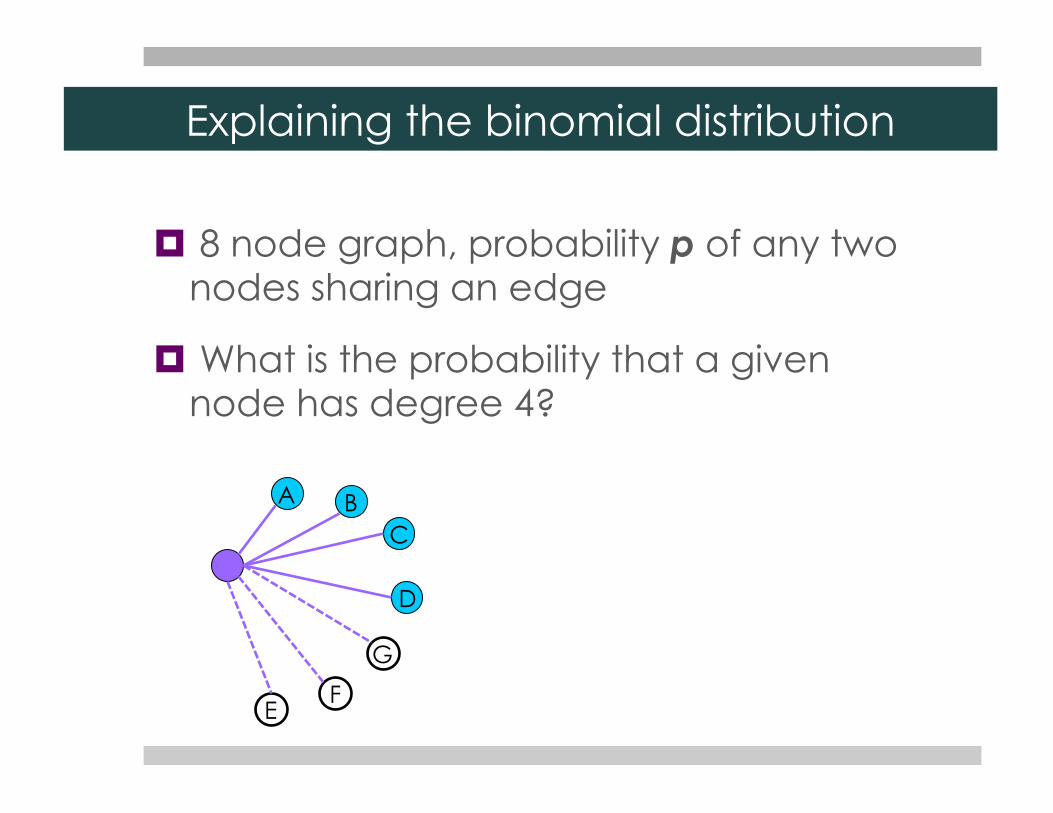
¤  8 node graph, probability p of any two nodes sharing an edge

¤  What is the probability that a given node has degree 4?

A B C

D

E F

G

Binomial coefficient: choosing 4 out of 7

A B C D E F G

Suppose I have 7 blue and white nodes, each of them uniquely marked so that I can distinguish them. The blue nodes are ones I share an edge with, the white ones I don’t.

A B C D E F G

How many different samples can I draw containing the same nodes but in a different order (the order could be e.g. the order in which the edges are added (or not)? e.g.

binomial coefficient explained

If order matters, there are 7! different orderings: I have 7 choices for the first spot, 6 choices for the second (since I’ve picked 1 and now have only 6 to choose from), 5 choices for the third, etc. 7! = 7 * 6 * 5 * 4 * 3 * 2 * 1

A B C D E F G

A B C D

Suppose the order of the nodes I don’t connect to (white) doesn’t matter. All possible arrangements (3!) of white nodes look the same to me. A B C D E F G

A B C D E G F

A B C D F E G

A B C D F G E

A B C D G F E

A B C D G E F

Instead of 7! combinations, we have 7!/3! combinations

binomial coefficient

F E G

The same goes for the blue nodes, if we can’t tell them apart, we lose a factor of 4!


= ----------------------------------------------------------------- number of ways of arranging n-1 items

(# of ways to arrange k things)*(# ways to arrange n-1-k things)

= ----------------- n-1! k! (n-1-k)!

Note that the binomial coefficient is symmetric – there are the same number of ways of choosing k or n-1-k things out of n-1


number of ways of choosing k items out of (n-1)

Quiz Q:

¤  What is the number of ways of choosing 2 items out of 5? ¤ 10 ¤ 120 ¤ 6 ¤ 5

Now the distribution

¤ p = probability of having edge to node (blue) ¤ (1-p) = probability of not having edge (white) ¤ The probability that you connect to 4 of the 7 nodes in

some particular order (two white followed by 3 blues, followed by a white followed by a blue) is P(white)*P(white)*P(blue)*P(blue)*P(blue)*P(white)*P(blue) = p4*(1-p)3

Binomial distribution

¤ If order doesn’t matter, need to multiply probability of any given arrangement by number of such arrangements:

+ ….

B(7;4; p) = 74

!

"#

$

%& p4 (1− p)3

if p = 0.5

p = 0.1

What is the mean?

¤ Average degree <k>= z = (n-1)*p

¤ in general µ = E(X) = Σx p(x)

0 * + 1 * + 2 * + 3 * + 4 * + 5 * + 6 * + 7 *

0.00

0.

05

0.10

0.

15

0.20

0.

25

probabilities that sum to 1

µ = 3.5

Quiz Q:

¤ What is the average degree of a graph with 10 nodes and probability p = 1/3 of an edge existing between any two nodes? ¤  1 ¤  2 ¤  3 ¤  4

What is the variance?

¤  variance in degree σ2=(n-1)*p*(1-p)

¤  in general σ2 = E[(X-µ)2] = Σ (x-µ)2 p(x)

(-3.5)2 * + + + + + +

0.00

0.

05

0.10

0.

15

0.20

0.

25

probabilities that sum to 1

(-2.5)2 *

+

(-1.5)2 *

(-0.5)2 * (0.5)2 *

(1.5)2 *

(2.5)2 * (-3.5)2 *

Approximations

knkk pp

kn

p −−−⎟⎟⎠

⎞⎜⎜⎝

⎛ −= 1)1(

1Binomial

Poisson

Normal

limit p small

limit large n

!kezpzk

k

−

=

pk =1

σ 2πe−(k−z)2

2σ 2

Poisson distribution

Poisson distribution

What insights does this yield? No hubs

¤  You don’t expect large hubs in the network

Insights

¤  Previously: degree distribution / absence of hubs

¤ Emergence of giant component

¤ Average shortest path

Emergence of the giant component

(standard model in NetLogo library) http://ccl.northwestern.edu/netlogo/models/GiantComponent

Quiz Q:

¤ What is the average degree z at which the giant component starts to emerge? ¤ 0 ¤ 1 ¤ 3/2 ¤ 3

Percolation on a 2D lattice

http://web.stanford.edu/class/cs224w/NetLogo/LatticePercolation.nlogo

Quiz Q:

¤ What is the percolation threshold of a 2D lattice: fraction of sites that need to be occupied in order for a giant connected component to emerge? ¤ 0 ¤ ¼ ¤ 1/3 ¤ 1/2

average degree

size

of g

iant

com

pone

nt

Percolation threshold

av deg = 0.99 av deg = 1.18 av deg = 3.96

Percolation threshold: how many edges need to be added before the giant component appears? As the average degree increases to z = 1, a giant component suddenly appears

“Evolution” of the Gnp

What happens to Gnp when we vary p?

Back to Node Degrees of Gnp

¤ Remember, expected degree

¤ If want E[Xv] be independent of n

let: p=c/(n-1)

pnXE v )1(][ −=

Probability of a node being isolated

¤ Observation: If we build random graph Gnp with p=c/(n-1) we have many isolated nodes

¤ Why?

38

c

n

nn e

ncpvP −

∞→

−− →⎟

⎠

⎞⎜⎝

⎛−

−=−=1

1

11)1(]0 degree has [

c

cx

x

cxn

ne

xxnc −

−−

∞→

⋅−−

∞→

=⎥⎥⎦

⎤

⎢⎢⎣

⎡⎟⎠

⎞⎜⎝

⎛ −=⎟⎠

⎞⎜⎝

⎛ −=⎟⎠

⎞⎜⎝

⎛−

−1111

11 limlim

1

11

−=nc

xUse substitution e (by definition)

No Isolated Nodes ¤ How big do we have to make p before we

are likely to have no isolated nodes?

¤ We know: P[v has degree 0] = e-c

¤ Event we are asking about is: ¤ I = some node is isolated ¤  where Iv is the event that v is isolated

¤ We have:

39

∪Nv

vII∈

=

( ) ( )∑∈∈

−=≤⎟⎟⎠

⎞⎜⎜⎝

⎛=

Nvv

Nvv

cneIPIPIP ∪

Union bound

∑≤i

ii

i AA∪

Ai

No Isolated Nodes

¤ We just learned: P(I) = n e-c

¤ Let’s try: ¤ c = ln n then: n e-c = n e-ln n =n⋅1/n= 1 ¤ c = 2 ln n then: n e-2 ln n = n⋅1/n2 = 1/n

¤ So if: ¤ p = ln n then: P(I) = 1 ¤ p = 2 ln n then: P(I) = 1/n → 0 as n→∞

Jure Leskovec, Stanford CS224W: Social and Information Network Analysis, http://cs224w.stanford.edu 40

“Evolution” of a Random Graph

¤ Graph structure of Gnp as p changes:

¤ Emergence of a Giant Component:

avg. degree k=2E/n or p=k/(n-1) ¤ k=1-ε: all components are of size Ω(log n) ¤ k=1+ε: 1 component of size Ω(n), others have size Ω(log n)

Jure Leskovec, Stanford CS224W: Social and Information Network Analysis, http://cs224w.stanford.edu 41

0 1 p

1/(n-1) Giant component

appears

c/(n-1) Avg. deg const. Lots of isolated

nodes.

log(n)/(n-1) Fewer isolated

nodes.

2*log(n)/(n-1) No isolated nodes.

Empty graph

Complete graph

Giant component – another angle

¤  How many other friends besides you does each of your friends have?

¤  By property of degree distribution ¤ the average degree of your friends, you

excluded, is z ¤ so at z = 1, each of your friends is expected to

have another friend, who in turn have another friend, etc.

¤ the giant component emerges

Giant component illustrated

Why just one giant component?

¤ What if you had 2, how long could they be sustained as the network densifies?

http://web.stanford.edu/class/cs224w/NetLogo/ErdosRenyiTwoComponents.nlogo

Quiz Q:

¤ If you have 2 large-components each occupying roughly 1/2 of the graph, how long does it typically take for the addition of random edges to join them into one giant component ¤ 1-4 edge additions ¤ 5-20 edge additions ¤ over 20 edge additions

Average shortest path

¤  How many hops on average between each pair of nodes?

¤  again, each of your friends has z = avg. degree friends besides you

¤  ignoring loops, the number of people you have at distance l is

zl

Average shortest path

friends at distance l

Nl=zl

scaling: average shortest path lav

lav ~logNlog z

What this means in practice

¤  Erdös-Renyi networks can grow to be very large but nodes will be just a few hops apart

0 200000 400000 600000 800000 1000000

05

1015

20

num nodes

aver

age

shor

test

pat

h

Logarithmic axes ¤ powers of a number will be uniformly spaced

1 2 3 10 20 30 100 200

n  20=1, 21=2, 22=4, 23=8, 24=16, 25=32, 26=64,….

Erdös-Renyi avg. shortest path

1 100 10000 1000000

05

1015

20

num nodes

aver

age

shor

test

pat

h

Quiz Q:

¤ If the size of an Erdös-Renyi network increases 100 fold (e.g. from 100 to 10,000 nodes), how will the average shortest path change ¤  it will be 100 times as long ¤  it will be 10 times as long ¤  it will be twice as long ¤  it will be the same ¤  it will be 1/2 as long

Realism

¤  Consider alternative mechanisms of constructing a network that are also fairly “random”.

¤  How do they stack up against Erdös-Renyi?

¤ http://web.stanford.edu/class/cs224w/NetLogo/RandomGraphs.nlogo

Introduction model

¤  Prob-link is the p (probability of any two nodes sharing an edge) that we are used to

¤  But, with probability prob-intro the other node is selected among one of our friends’ friends and not completely at random

Introduction model

Quiz Q:

¤  Relative to ER, the introduction model has: ¤ more edges ¤ more closed triads ¤  longer average shortest path ¤ more uneven degree ¤ smaller giant component at low p

Static Geographical model

¤  Each node connects to num-neighbors of its closest neighbors

¤  use the num-neighbors slider, and for comparison, switch PROB-OR-NUM to ‘off’ to have the ER model aim for num-neighbors as well

¤  turn off the layout algorithm while this is running, you can apply it at the end

static geo

Quiz Q:

¤  Relative to ER, the static geographical model has : ¤  longer average shortest path ¤ shorter average shortest path ¤ narrower degree distribution ¤ broader degree distribution ¤ smaller giant component at a low number of

neighbors ¤  larger giant component at a low number of

neighbors

Random encounter

¤ People move around randomly and connect to people they bump into


¤  turn off the layout algorithm while this is running (you can apply it at the end)

random encounters

Quiz Q:

¤  Relative to ER, the random encounters model has : ¤ more closed triads ¤ fewer closed triads ¤ smaller giant component at a low number of


neighbors

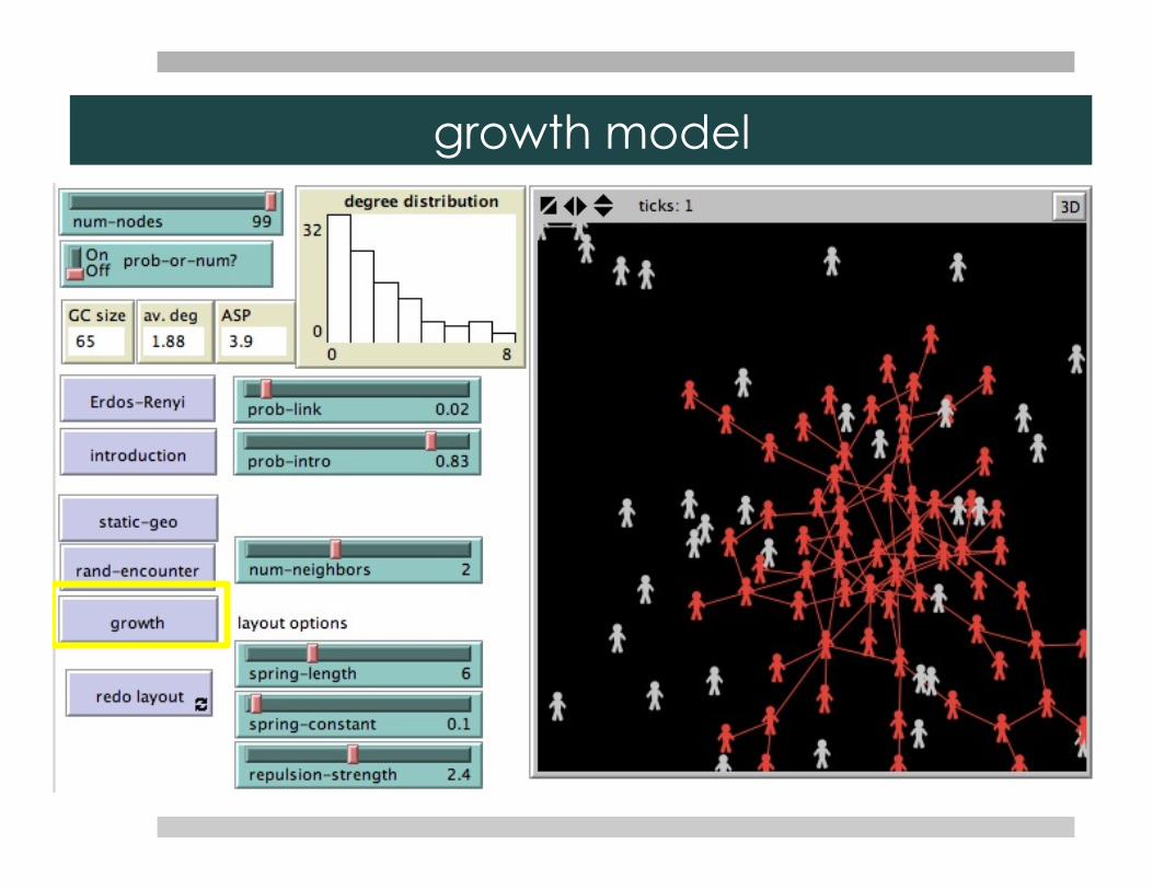
Growth model

¤ Instead of starting out with a fixed number of nodes, nodes are added over time


growth model

Quiz Q:

¤  Relative to ER, the growth model has : ¤ more hubs ¤ fewer hubs ¤ smaller giant component at a low number of


neighbors

other models

¤  in some instances the ER model is plausible

¤  if dynamics are different, ER model may be a poor fit

random graphs - stanford...

Documents