INVERSE PROBLEMS IN

IMAGE PROCESSING

Ramesh Neelamani

Thesis: Doctor of PhilosophyElectrical and Computer EngineeringRice University, Houston, Texas (June 2003)

RICE UNIVERSITY

Inverse Problems in Image Processing

by

Ramesh Neelamani

A THESIS SUBMITTED

IN PARTIAL FULFILLMENT OF THE

REQUIREMENTS FOR THE DEGREE

Doctor of Philosophy

APPROVED, THESIS COMMITTEE:

Richard Baraniuk, Professor, ChairElectrical and Computer Engineering

Robert Nowak, Associate ProfessorElectrical and Computer Engineering

Michael Orchard, ProfessorElectrical and Computer Engineering

Steven J. Cox, ProfessorComputational and Applied Mathematics

HOUSTON, TEXAS

JUNE 2003

Inverse Problems in Image Processing

Ramesh Neelamani

Abstract

Inverse problems involve estimating parameters or data from inadequate observations; the obser-

vations are often noisy and contain incomplete information about the target parameter or data due

to physical limitations of the measurement devices. Consequently, solutions to inverse problems

are non-unique. To pin down a solution, we must exploit the underlying structure of the desired so-

lution set. In this thesis, we formulate novel solutions to three image processing inverse problems:

deconvolution, inverse halftoning, and JPEG compression history estimation for color images.

Deconvolution aims to extract crisp images from blurry observations. We propose an effi-

cient, hybrid Fourier-Wavelet Regularized Deconvolution (ForWaRD) algorithm that comprises

blurring operator inversion followed by noise attenuation via scalar shrinkage in both the Fourier

and wavelet domains. The Fourier shrinkage exploits the structure of the colored noise inherent in

deconvolution, while the wavelet shrinkage exploits the piecewise smooth structure of real-world

signals and images. ForWaRD yields state-of-the-art mean-squared-error (MSE) performance in

practice. Further, for certain problems, ForWaRD guarantees an optimal rate of MSE decay with

increasing resolution.

Halftoning is a technique used to render gray-scale images using only black or white dots. In-

verse halftoning aims to recover the shades of gray from the binary image and is vital to process

scanned images. Using a linear approximation model for halftoning, we propose the Wavelet-

based Inverse Halftoning via Deconvolution (WInHD) algorithm. WInHD exploits the piece-wise

smooth structure of real-world images via wavelets to achieve good inverse halftoning perfor-

mance. Further, WInHD also guarantees a fast rate of MSE decay with increasing resolution.

We routinely encounter digital color images that were previously JPEG-compressed. We aim to

retrieve the various settings—termed JPEG compression history—employed during previous JPEG

operations. This information is often discarded en-route to the image’s current representation. We

discover that the previous JPEG compression’s quantization step introduces lattice structures into

the image. Our study leads to a fundamentally new result in lattice theory—nearly orthogonal sets

of lattice basis vectors contain the lattice’s shortest non-zero vector. We exploit this insight along

with other known, novel lattice-based algorithms to effectively uncover the image’s compression

history. The estimated compression history significantly improves JPEG recompression.

Acknowledgments

I am indebted to my energetic advisor and mentor Prof. Richard Baraniuk for making my Rice

experience truly enjoyable and enlightening. I am also grateful to my other thesis committee mem-

bers Prof. Robert Nowak, Prof. Michael Orchard, and Prof. Steven Cox for stimulating discussions

and valuable comments.

All my research collaborators, including Richard Baraniuk, Kathrin Berkner, Hyeokho Choi,

Sanjeeb Dash, Zhigang Fan, Robert Nowak, Ricardo de Queiroz, Rudolf Riedi, and

Justin Romberg, have played a critical role in broadening my research horizons. I truly ap-

preciate the enthusiasm and the seemingly-infinite patience they displayed while interacting with

me.

Thanks to all my friends and the Rice ECE group of professors and students for keeping me

bright and sunny. I now have a home away from home.

I lack words to express my gratitude to amma, appa, and Anu for their unconditional love and

support.

Sandhya has made this journey worthwhile.

Contents

Abstract ii

Acknowledgments iv

1 Introduction 1

1.1 ForWaRD: Fourier-Wavelet Regularized Deconvolution . . . . . . . . . . . . . . . 2

1.2 WInHD: Wavelet-based Inverse Halftoning via Deconvolution . . . . . . . . . . . 3

1.3 JPEG Compression History Estimation (CHEst) for Color Images . . . . . . . . . 4

2 ForWaRD: Fourier-Wavelet Regularized Deconvolution 6

2.1 Introduction . . . . . . . . . . . . . . . . . . . . . . . . . . . . . . . . . . . . . . 6

2.1.1 Problem statement . . . . . . . . . . . . . . . . . . . . . . . . . . . . . . 6

2.1.2 Transform-domain shrinkage . . . . . . . . . . . . . . . . . . . . . . . . . 8

2.1.3 Fourier-Wavelet Regularized Deconvolution (ForWaRD) . . . . . . . . . . 11

2.1.4 Related work . . . . . . . . . . . . . . . . . . . . . . . . . . . . . . . . . 14

2.1.5 Chapter organization . . . . . . . . . . . . . . . . . . . . . . . . . . . . . 15

2.2 Sampling and Deconvolution . . . . . . . . . . . . . . . . . . . . . . . . . . . . . 15

2.3 Fourier-based Regularized Deconvolution (FoRD) . . . . . . . . . . . . . . . . . 18

2.3.1 Framework . . . . . . . . . . . . . . . . . . . . . . . . . . . . . . . . . . 18

2.3.2 Strengths of FoRD . . . . . . . . . . . . . . . . . . . . . . . . . . . . . . 20

vi

2.3.3 Limitations of FoRD . . . . . . . . . . . . . . . . . . . . . . . . . . . . . 20

2.4 Wavelet-Vaguelette Deconvolution (WVD) . . . . . . . . . . . . . . . . . . . . . 21

2.4.1 Framework . . . . . . . . . . . . . . . . . . . . . . . . . . . . . . . . . . 21

2.4.2 Strengths of WVD . . . . . . . . . . . . . . . . . . . . . . . . . . . . . . 21

2.4.3 Limitations of WVD . . . . . . . . . . . . . . . . . . . . . . . . . . . . . 22

2.5 Fourier-Wavelet Regularized Deconvolution (ForWaRD) . . . . . . . . . . . . . . 22

2.5.1 ForWaRD algorithm . . . . . . . . . . . . . . . . . . . . . . . . . . . . . 23

2.5.2 How ForWaRD works . . . . . . . . . . . . . . . . . . . . . . . . . . . . 23

2.5.3 Balancing Fourier and wavelet shrinkage in ForWaRD . . . . . . . . . . . 24

2.5.4 Asymptotic ForWaRD performance and optimality . . . . . . . . . . . . . 29

2.6 ForWaRD Implementation . . . . . . . . . . . . . . . . . . . . . . . . . . . . . . 35

2.6.1 Estimation of σ2 . . . . . . . . . . . . . . . . . . . . . . . . . . . . . . . 35

2.6.2 Choice of Fourier shrinkage . . . . . . . . . . . . . . . . . . . . . . . . . 35

2.6.3 Choice of wavelet basis and shrinkage . . . . . . . . . . . . . . . . . . . . 36

2.7 Results . . . . . . . . . . . . . . . . . . . . . . . . . . . . . . . . . . . . . . . . . 37

2.7.1 Simulated problem . . . . . . . . . . . . . . . . . . . . . . . . . . . . . . 37

2.7.2 Real-life application: Magnetic Force Microscopy . . . . . . . . . . . . . 38

3 WInHD: Wavelet-based Inverse Halftoning via Deconvolution 41

3.1 Introduction . . . . . . . . . . . . . . . . . . . . . . . . . . . . . . . . . . . . . . 41

3.2 Linear Model for Error Diffusion . . . . . . . . . . . . . . . . . . . . . . . . . . . 46

3.3 Inverse Halftoning ≈ Deconvolution . . . . . . . . . . . . . . . . . . . . . . . . . 48

3.3.1 Deconvolution . . . . . . . . . . . . . . . . . . . . . . . . . . . . . . . . 49

vii

3.3.2 Inverse halftoning via Gaussian low-pass filtering (GLPF) . . . . . . . . . 52

3.4 Wavelet-based Inverse Halftoning Via Deconvolution (WInHD) . . . . . . . . . . 53

3.4.1 WInHD algorithm . . . . . . . . . . . . . . . . . . . . . . . . . . . . . . 53

3.4.2 Asymptotic performance of WInHD . . . . . . . . . . . . . . . . . . . . . 55

3.5 Results . . . . . . . . . . . . . . . . . . . . . . . . . . . . . . . . . . . . . . . . . 57

4 JPEG Compression History Estimation (CHEst) for Color Images 60

4.1 Introduction . . . . . . . . . . . . . . . . . . . . . . . . . . . . . . . . . . . . . . 60

4.2 Color Spaces and Transforms . . . . . . . . . . . . . . . . . . . . . . . . . . . . . 63

4.3 JPEG Overview . . . . . . . . . . . . . . . . . . . . . . . . . . . . . . . . . . . . 65

4.4 CHEst for Gray-Scale Images . . . . . . . . . . . . . . . . . . . . . . . . . . . . 66

4.4.1 Statistical framework . . . . . . . . . . . . . . . . . . . . . . . . . . . . . 67

4.4.2 Algorithm steps . . . . . . . . . . . . . . . . . . . . . . . . . . . . . . . . 69

4.5 Dictionary-based CHEst for Color Images . . . . . . . . . . . . . . . . . . . . . . 70

4.5.1 Statistical framework . . . . . . . . . . . . . . . . . . . . . . . . . . . . . 70

4.5.2 Algorithm steps . . . . . . . . . . . . . . . . . . . . . . . . . . . . . . . . 71

4.5.3 Dictionary-based CHEst results . . . . . . . . . . . . . . . . . . . . . . . 72

4.6 Blind Lattice-based CHEst for Color Images . . . . . . . . . . . . . . . . . . . . . 74

4.6.1 Ideal lattice structure of DCT coefficients . . . . . . . . . . . . . . . . . . 76

4.6.2 Lattice algorithms . . . . . . . . . . . . . . . . . . . . . . . . . . . . . . 78

4.6.3 LLL provides parallelepiped lattice’s basis vectors . . . . . . . . . . . . . 83

4.6.4 Estimating scaled linear component of the color transform . . . . . . . . . 84

4.6.5 Estimating the complete color transform and quantization step-sizes . . . . 86

viii

4.6.6 Round-offs perturb ideal geometry . . . . . . . . . . . . . . . . . . . . . . 87

4.6.7 Combating round-off noise . . . . . . . . . . . . . . . . . . . . . . . . . . 88

4.6.8 Algorithm steps . . . . . . . . . . . . . . . . . . . . . . . . . . . . . . . . 90

4.6.9 Lattice-based CHEst results . . . . . . . . . . . . . . . . . . . . . . . . . 92

4.7 JPEG Recompression: A Sample Application of CHEst . . . . . . . . . . . . . . . 95

4.7.1 JPEG recompression using dictionary-based CHEst . . . . . . . . . . . . . 95

4.7.2 JPEG recompression using lattice-based CHEst . . . . . . . . . . . . . . . 97

5 Conclusions 99

A Background on Wavelets 104

A.1 1-D and 2-D Wavelet Transforms . . . . . . . . . . . . . . . . . . . . . . . . . . . 104

A.2 Economy of Wavelet Representations . . . . . . . . . . . . . . . . . . . . . . . . 106

A.3 Wavelet Shrinkage-based Signal Estimation . . . . . . . . . . . . . . . . . . . . . 107

B Formal WVD Algorithm 109

C Derivation of Optimal Regularization Parameters for ForWaRD 111

D Decay Rate of Wavelet Shrinkage Error in ForWaRD 113

D.1 Besov Smoothness of Distorted Signal . . . . . . . . . . . . . . . . . . . . . . . . 113

D.2 Wavelet-domain Estimation Error: ForWaRD vs. Signal in White Noise . . . . . . 114

E Decay Rate of Total ForWaRD MSE 116

ix

E.1 Bounding Wavelet Shrinkage Error . . . . . . . . . . . . . . . . . . . . . . . . . . 116

E.2 Bounding Fourier Distortion Error . . . . . . . . . . . . . . . . . . . . . . . . . . 116

F Decay Rate of WInHD’s MSE 119

G Properties of Nearly Orthogonal Basis Vectors 120

G.1 Proof of Proposition 5 . . . . . . . . . . . . . . . . . . . . . . . . . . . . . . . . . 120

G.1.1 Proof for 2-D lattices . . . . . . . . . . . . . . . . . . . . . . . . . . . . . 120

G.1.2 Proof for higher dimensional lattices . . . . . . . . . . . . . . . . . . . . . 121

G.2 Proof of Proposition 6 . . . . . . . . . . . . . . . . . . . . . . . . . . . . . . . . . 122

G.2.1 Proof for 2-D lattices . . . . . . . . . . . . . . . . . . . . . . . . . . . . . 122

G.2.2 Proof for higher dimensional lattices . . . . . . . . . . . . . . . . . . . . . 124

Bibliography 128

1

Chapter 1

Introduction

There was neither non-existence nor existence then;

there was neither the realm of space nor the sky which is beyond.

–From the Rig Veda (translated by Prof. W. D. O’Flaherty)

Inverse problems estimate some parameter or data from a set of indirect noisy observations.

Due to lack of sufficient information in the indirect observations, solutions to inverse problems are

typically non-unique and, therefore, challenging. To tackle the inherent ambiguity of inverse prob-

lems solutions, we need to incorporate into our estimation a priori information about the structure

of desired solution set.

In this thesis, we formulate solutions to deconvolution, inverse halftoning, and JPEG Compres-

sion History Estimation (CHEst) for color images. We constrain our deconvolution and inverse

halftoning solutions by using wavelet representations to exploit the piece-wise smooth structure of

typical real-world signals and images. JPEG’s quantization operation creates lattice structures in

the discrete cosine transform (DCT) coefficients. We exploit these lattice structures using novel

algorithms from cryptography to perform color image JPEG CHEst.

2

1.1 ForWaRD: Fourier-Wavelet Regularized Deconvolution

Given an observation that is comprised of an input image first degraded by linear time-invariant

(LTI) convolution with a known impulse response and then corrupted by additive noise, deconvo-

lution aims to estimate the input image. Deconvolution is extremely important in applications such

as satellite imaging and seismic imaging.

To solve the deconvolution problem, in Chapter 2, we propose a fast hybrid algorithm called

Fourier-wavelet regularized deconvolution (ForWaRD) that comprises of convolution operator in-

version followed by scalar shrinkage in both the Fourier domain and the wavelet domain. The

Fourier shrinkage exploits the Fourier transform’s economical representation of the colored noise

inherent in deconvolution, while the wavelet shrinkage exploits the wavelet domain’s economical

representation of piecewise smooth signals and images. We derive the optimal balance between

the amount of Fourier and wavelet regularization by optimizing an approximate mean-squared-

error (MSE) metric and find that signals with more economical wavelet representations require

less Fourier shrinkage. ForWaRD is applicable to all ill-conditioned deconvolution problems, un-

like the purely wavelet-based Wavelet-Vaguelette Deconvolution (WVD); moreover, its estimate

features minimal ringing, unlike the purely Fourier-based Wiener deconvolution. Even in prob-

lems for which the WVD was designed, we prove that ForWaRD’s MSE decays with the optimal

WVD rate as the number of samples increases. Further, we demonstrate that over a wide range of

practical sample-lengths, ForWaRD improves upon WVD’s performance.

3

1.2 WInHD: Wavelet-based Inverse Halftoning via Deconvolution

Digital halftoning is a common technique used to render a sampled gray-scale image using only

black or white dots [1] (see Figures 3.3(a) and (b)); the rendered bi-level image is referred to as a

halftone. Inverse halftoning is the process of retrieving a gray-scale image from a given halftone.

Applications of inverse halftoning include enhancement and compression of facsimile images [2].

We propose a novel algorithm called Wavelet-based inverse halftoning via deconvolution

(WInHD) to perform inverse halftoning of error-diffused halftones in Chapter 3. We realize that in-

verse halftoning can be formulated as a deconvolution problem by using the linear approximation

model for error diffusion halftoning of Kite et al. In the linear approximation model, the error-

diffused halftone is modeled as the gray-scale input blurred by a convolution operator and cor-

rupted with additive colored noise; the convolution operator and noise coloring are determined by

the error diffusion technique. WInHD adopts a wavelet-based deconvolution approach to perform

inverse halftoning; it by first inverts the model-specified convolution operator and then attenuates

the residual noise using scalar wavelet-domain operations. Since WInHD is model-based, it is

easily adapted to different error diffusion halftoning techniques. Unlike previous inverse halfton-

ing algorithms, under mild assumptions, we derive for images in a Besov space the minimum rate

at which the WInHD estimate’s MSE decays as the spatial resolution of the gray-scale image in-

creases (i.e., number of samples→∞). We also prove that WInHD’s MSE decay rate is optimal if

the gray-scale image before halftoning is noisy. Using simulations, we verify that WInHD is com-

petitive with state-of-the-art inverse halftoning techniques in the mean square error (MSE) sense

and it also provides good visual performance.

4

1.3 JPEG Compression History Estimation (CHEst) for Color Images

We routinely encounter digital color images in bitmap (BMP) formats or in lossless compression

formats such as Tagged Image File Format (TIFF). Such images are often subjected to JPEG (Joint

Photographic Experts Group) compression and decompression operations before reaching their

current representation. The settings used during the previous JPEG compression and decompres-

sion; such as the choice of color transformation, subsampling, and the quantization table; is not

standardized [3]. We refer to such previous JPEG compression settings as the image’s JPEG com-

pression history. The compression history is lost during operations such as conversion from JPEG

format to BMP or TIFF format. We aim to estimate this lost information from the image’s current

representation. The estimated JPEG compression history can be used for JPEG recompression, for

covert message passing, or to uncover the compression settings used inside digital cameras.

In Chapter 4, we propose a new framework to estimate the compression history of color images.

Due to quantization and dequantization operations during JPEG compression and decompression,

the discrete cosine transform (DCT) coefficient histograms of previously JPEG-compressed im-

ages exhibit near-periodic structure with the period determined by the quantization step-size. For

the general case, we derive a maximum likelihood approach that exploits the near-periodic DCT

coefficient structure to select the compression color space from a dictionary of color spaces and to

estimate the quantization table. If the transform from the color space used for JPEG compression

to the current color space is affine and if no subsampling is employed during JPEG compression,

then we no longer need a dictionary of color spaces to estimate the compression history. In this

special case, we demonstrate that the DCT coefficients of the observed image nearly conform to

a 3-dimensional parallelepiped lattice structure determined by the affine color transform. During

5

our study of lattices, we discover a new, fundamental property. We realize that a set of nearly

orthogonal lattice basis vectors always contains the shortest non-zero vector in the lattice. Further,

we also identify the conditions under which the set of nearly orthogonal basis vectors for a lattice

is unique. Using our new insights and with novel applications of existing lattice algorithms, we

exploit the lattice structure offered by our problem and estimate a color image’s JPEG compres-

sion history, namely, the affine color transform and the quantization tables. We demonstrate the

efficacy of our proposed algorithm via simulations. Further, we verify the utility of the estimated

compression history in JPEG recompression; we demonstrate that the estimated information allows

us to recompress an image with minimal distortion (large signal-to-noise-ratio) and simultaneously

achieve a small file-size.

6

Chapter 2

ForWaRD: Fourier-Wavelet Regularized Deconvolution

You can’t depend on your eyes when your imagination is out of focus.

–Mark Twain

2.1 Introduction

Deconvolution is a recurring theme in a wide variety of signal and image processing problems.

For example, practical satellite images are often blurred due to limitations such as aperture effects

of the camera, camera motion, or atmospheric turbulence [4]. Deconvolution becomes necessary

when we wish a crisp deblurred image for viewing or further processing.

2.1.1 Problem statement

In this chapter, we treat the classical discrete-time deconvolution problem. The problem setup and

solutions are described in 1-dimension (1-D), but everything extends directly to higher dimensions

as well. The observed samples y(n) consist of unknown desired signal samples x(n) first degraded

by circular convolution (denoted by ~) with a known impulse response h(n) from a linear time-

invariant (LTI) systemH and then corrupted by zero-mean additive white Gaussian noise (AWGN)

7

- ������

-

6

-

noiseγ

LTI systemH

observationy

desiredx

Figure 2.1: Convolution model setup. The observation y consists of the desired signal x firstdegraded by the linear time-invariant (LTI) convolution system H and then corrupted by zero-mean additive white Gaussian noise (AWGN) γ.

γ(n) with variance σ2 (see Fig. 2.1)

y(n) := Hx(n) + γ(n), n = 0, . . . , N − 1

:= (h~ x)(n) + γ(n). (2.1)

Given y and h, we seek to estimate x.

A naive deconvolution estimate x is obtained using the operator inverse H−1 as1

x(n) := H−1y(n) = x(n) +H−1γ(n). (2.2)

Unfortunately, the variance of the colored noise H−1γ in x is large when H is ill-conditioned. In

such a case, the mean-squared error (MSE) between x and x is large, making x an unsatisfactory

deconvolution estimate.

In general, deconvolution algorithms can be interpreted as estimating x from the noisy signal

x in (2.2). In this chapter, we focus on simple and fast estimation based on scalar shrinkage of

1For non-invertibleH, we replace H−1 by its pseudo-inverse and x by its orthogonal projection onto the range ofH in (2.2) [5]. The estimate x in (2.2) continues to retain all the information that y contains about x.

8

wavelets

Fourier

nois

e co

mpo

nent

ene

rgy

(dB

)

sorted component index

Fourier

wavelets

sign

al c

ompo

nent

ene

rgy

(dB

)

sorted component index

(a) colored noise 〈H−1γ, bk〉 (b) signal 〈x, bk〉

Figure 2.2: Economy of Fourier vs. wavelet representations. (a) Energies in dB of the Fourierand wavelet components of the noise H−1γ colored by the pseudo-inverse of a 2-D 9×9 box-carsmoothing operator. The components are sorted in descending order of energy from left to right.The colored noise energy is concentrated in fewer Fourier components than wavelet components.(b) Energies of the Fourier and wavelet components of the Cameraman image x. The signal energyis concentrated in fewer wavelet components than Fourier components.

individual components in a suitable transform domain. Such a focus is not restrictive because

transform-domain scalar shrinkage lies at the core of many traditional [6, 7] and modern [5, 8]

deconvolution approaches.

2.1.2 Transform-domain shrinkage

Given an orthonormal basis {bk}N−1k=0 for RN , the naive estimate x from (2.2) can be expressed as

x =

N−1∑

k=0

(〈x, bk〉+ 〈H−1γ, bk〉

)bk. (2.3)

9

An improved estimate xλ can be obtained by simply shrinking the k-th component in (2.3) with a

scalar λk, 0 ≤ λk ≤ 1 [9]:

xλ :=N−1∑

k=0

(〈x, bk〉+ 〈H−1γ, bk〉

)λk bk (2.4)

=: xλ +H−1γλ. (2.5)

The xλ :=∑

k〈x, bk〉λk bk denotes the retained part of the signal x that the shrinkage preserves

from (2.2), while H−1γλ :=∑

k〈H−1γ, bk〉λk bk denotes the leaked part of the colored noise

H−1γ that the shrinkage fails to attenuate. Clearly, we should set λk ≈ 1 if the variance σ2k :=

E(|〈H−1γ, bk〉|2) of the k-th colored noise component is small relative to the energy |〈x, bk〉|2 of

the corresponding signal component and set λk ≈ 0 otherwise. The shrinkage by λk can also be

interpreted as a form of regularization for the deconvolution inverse problem [7].

The tradeoff associated with the choice of λk is easily understood: If λk ≈ 1, then most of the

k-th colored noise component leaks into xλ with the corresponding signal component; the result is

a distortion-free but noisy estimate. In contrast, if λk ≈ 0, then most of the k-th signal component

is lost with the corresponding colored noise component; the result is a noise-free but distorted

estimate. Since the variance of the leaked noise H−1γλ in (2.5) and the energy of the lost signal

x − xλ comprise the MSE of the shrunk estimate xλ, judicious choices of the λk’s help lower the

estimate’s MSE.

However, an important fact is that for a given transform domain, even with the best possible

10

λk’s, the estimate xλ’s MSE is lower bounded by [8, 10, 11]

1

2

N−1∑

k=0

min(|〈x, bk〉|2, σ2

k

). (2.6)

From (2.6), xλ has small MSE only when most of the signal energy (=∑

k |〈x, bk〉|2) and colored

noise energy (=∑

k σ2k) is captured by just a few transform-domain coefficients—we term such

a representation economical—and when the energy-capturing coefficients for the signal and noise

are different. Otherwise, the xλ is either excessively noisy due to leaked noise components or

distorted due to lost signal components.

Traditionally, the Fourier domain (with sinusoidal bk) is used to estimate x from x. For ex-

ample, the LTI Wiener deconvolution filter corresponds to (2.4) with each λk determined by the

k-th component signal-to-noise ratio [6, 7]. The strength of the Fourier basis is that it most eco-

nomically represents the colored noise H−1γ (see Figure 2.2(a) and Section 2.3.2 for the details).

However, the weakness of the Fourier domain is that it does not economically represent signals

x with singularities such as images with edges (see Figure 2.2(b)). Consequently, as dictated by

the MSE bound in (2.6), any estimate obtained via Fourier shrinkage is unsatisfactory with a large

MSE; the estimate is either noisy or distorted for signals x with singularities (see Figure 2.4(c), for

example).

Recently, the wavelet domain (with bk shifts and dilates of a mother wavelet function) has been

exploited to estimate x from x; for example, Donoho’s Wavelet-Vaguelette Deconvolution (WVD)

[8]. The strength of the wavelet domain is that it economically represents classes of signals con-

taining singularities that satisfy a wide variety of local smoothness constraints, including piece-

wise smoothness and Besov space smoothness (see Figure 2.2(b) and Section 2.4.2 for the details).

11

inversion x

H−1

Fouriershrinkage

λf

xλf

- -- -observationy

waveletshrinkage

λw

ForWaRDestimate

x

Figure 2.3: Fourier-Wavelet Regularized Deconvolution (ForWaRD). ForWaRD employs a smallamount of Fourier shrinkage (most λf

k ≈ 1) to partially attenuate the noise amplified during opera-tor inversion. Subsequent wavelet shrinkage (determined by λw) effectively attenuates the residualnoise.

However, the weakness of the wavelet domain is that it typically does not economically represent

the colored noise H−1γ (see Figure 2.2(a)). Consequently, as dictated by the MSE bound in (2.6),

any estimate obtained via wavelet shrinkage is unsatisfactory with a large MSE; the estimate is

either noisy or distorted for many types of H.

Unfortunately, no single transform domain can economically represent both the noise colored

by a general H−1 and signals from a general smoothness class [8]. Hence, deconvolution tech-

niques employing shrinkage in a single transform domain cannot yield adequate estimates in many

deconvolution problems of interest.

2.1.3 Fourier-Wavelet Regularized Deconvolution (ForWaRD)

In this chapter, we propose a deconvolution scheme that relies on tandem scalar processing in

both the Fourier domain, which economically represents the colored noise H−1γ, and the wavelet

domain, which economically represents signals x from a wide variety of smoothness classes. Our

hybrid Fourier-Wavelet Regularized Deconvolution (ForWaRD) technique estimates x from x by

first employing a small amount of scalar Fourier shrinkage λf and then attenuating the leaked noise

with scalar wavelet shrinkage λw (see Fig. 2.3) [12, 13].

Here is how it works: During operator inversion, some Fourier coefficients of the noise γ are

12

significantly amplified; just a small amount of Fourier shrinkage (most λfk ≈ 1) is sufficient to

attenuate these amplified Fourier noise coefficients with minimal loss of signal components. The

leaked noiseH−1γλf that Fourier shrinkage λf fails to attenuate (see (2.5)) has significantly reduced

energy in all wavelet coefficients, but the signal part xλf that Fourier shrinkage retains continues

to be economically represented in the wavelet domain. Hence subsequent wavelet shrinkage effec-

tively extracts the retained signal xλf from the leaked noiseH−1γλf and provides a robust estimate.

For an idealized ForWaRD system, we will derive the optimal balance between the amount of

Fourier shrinkage and wavelet shrinkage by optimizing over an approximate MSE metric. We will

find that signals with more economical wavelet representations require less Fourier shrinkage.

Figure 2.4 illustrates the superior overall visual quality and lower MSE of the ForWaRD es-

timate as compared to the LTI Wiener filter estimate [6, 7] for the 2-D box-car blur operator,

which models rectangular scanning aperture effects [4], with impulse response h(n1, n2) = 181

for 0 ≤ n1, n2 ≤ 8 and 0 otherwise (see Section 2.7 for the details). For this operator, the WVD

approach returns a near-zero estimate; scalar wavelet shrinkage cannot salvage the signal compo-

nents since nearly all wavelet coefficients are corrupted with high-variance noise.

Indeed, even in problems for which the WVD was designed, we will prove that the ForWaRD

MSE also decays with the same optimal WVD rate as the number of samples increases. Further,

for such problems, we will experimentally demonstrate ForWaRD’s superior MSE performance

compared to the WVD over a wide range of practical sample sizes (see Fig. 2.6(a)).

13

(a) Desired x (b) Observed y

(c) LTI Wiener filter estimate (d) ForWaRD estimate

Figure 2.4: (a) Desired Cameraman image x (256 × 256 samples). (b) Observed image y: xsmoothed by a 2-D 9×9 box-car blur plus white Gaussian noise with variance such that the BSNR= 40 dB. (c) LTI Wiener filter estimate (SNR = 20.8 dB, ISNR = 5.6 dB). (d) ForWaRD estimate(SNR = 22.5 dB, ISNR = 7.3 dB). See Section 2.7 for further details.

14

2.1.4 Related work

Kalifa and Mallat have proposed a mirror-wavelet basis approach that is similar to the WVD but

employs scalar shrinkage in the mirror-wavelet domain adapted to the colored noise H−1γ instead

of shrinkage in the conventional wavelet domain [5]. Although the adapted basis improves upon

the WVD performance in some “hyperbolic” deconvolution problems, similarly to the WVD, it

provides inadequate estimates for arbitrary convolution operators. For example, for the ubiquitous

box-car blurH, again most signal components are lost during scalar shrinkage due to high-variance

noise. Figure 2.7(b) illustrates that ForWaRD is competitive with the mirror-wavelet approach even

for a hyperbolic deconvolution problem.

Similar to ForWaRD, Nowak and Thul [14] have first employed an under-regularized system

inverse and subsequently used wavelet-domain signal estimation. However, they do not address

the issue of optimal regularization or asymptotic performance.

Banham and Katsaggelos have applied a multiscale Kalman filter to the deconvolution problem

[15]. Their approach employs an under-regularized, constrained-least-squares prefilter to reduce

the support of the state vectors in the wavelet domain, thereby improving computational efficiency.

The amount of regularization chosen for each wavelet scale is the lower bound that allows for reli-

able edge classification. While similar in spirit to the multiscale Kalman filter approach, ForWaRD

employs simple Wiener or Tikhonov regularization in the Fourier domain to optimize the MSE per-

formance. Also, ForWaRD employs simple scalar shrinkage on the wavelet coefficients in contrast

to more complicated prediction on edge and non-edge quad-trees [15]. Consequently, as discussed

in Section 2.5.4, ForWaRD demonstrates excellent MSE performance as the number of samples

tends to infinity and is in fact asymptotically optimal in certain cases. Further, as demonstrated in

15

Section 2.7, ForWaRD yields better estimates than the multiscale Kalman filter approach.

There exists a vast literature on iterative deconvolution techniques; see [7, 16–18] and the ref-

erences therein. In this chapter, we focus exclusively on non-iterative techniques for the sake of

implementation speed and simplicity. Nevertheless, many iterative techniques could exploit the

ForWaRD estimate as a seed to initialize their iterations; for example, see [19].

2.1.5 Chapter organization

We begin by providing a more precise definition of the convolution setup (2.1) in Section 2.2.

We then discuss techniques that employ scalar Fourier shrinkage in Section 2.3. We introduce

the WVD technique in Section 2.4. We present the hybrid ForWaRD scheme in Section 2.5 and

discuss its practical implementation in Section 2.6. Illustrative examples lie in Section 2.7. A

short overview of wavelets in Appendix A, a WVD review in Appendix B, and technical proofs in

Appendices C–E complement this chapter.

2.2 Sampling and Deconvolution

Most real-life deconvolution problems originate in continuous time and are then sampled. In this

section, we sketch the relationship between such a sampled continuous-time setup and the setup

with discrete-time circular convolution considered in this chapter (see (2.1)).

Consider the following sampled continuous-time deconvolution setup: An unknown finite-

energy desired signal x(t) is blurred by linear convolution (denoted by ∗) with the known finite-

energy impulse response h(t) of an LTI system and then corrupted by an additive Gaussian process

γ(t) to form the observation z(t) = (h ∗ x)(t) + γ(t). For finite-support x(t) and h(t), the finite-

16

support (h ∗ x)(t) can be obtained using circular convolution with a sufficiently large period. For

infinite-support x(t) and h(t), the approximation of (h ∗ x)(t) using circular convolution can be

made arbitrarily precise by increasing the period. Hence, we assume that the observation z(t) over

a normalized unit interval can be obtained using circular convolution with a unit period, that is,

z(t) := (h~ x)(t) + γ(t) with t ∈ [0, 1). Deconvolution aims to estimate x(t) from the samples

z(n) of the continuous-time observation z(t). For example, z(n) can be obtained by averaging z(t)

over uniformly spaced intervals of length 1N

z(n) := N

∫ n+1

N

nN

z(t) dt, n = 0, . . . , N − 1. (2.7)

Other sampling kernels can also be used in (2.7);2 see [20, 21] for excellent tutorials on sampling.

Such a setup encapsulates many real-life deconvolution problems [4].

The observation samples z(n) from (2.7) can be closely approximated by the observation y(n)

from setup (2.1) [4], that is,

z(n) ≈ y(n) = (h~ x)(n) + γ(n), n = 0, . . . , N − 1, (2.8)

if the continuous-time variables x(t), γ(t), and h(t) comprising z(n) are judiciously related to

the discrete variables x(n), γ(n), and h(n) comprising y(n). We choose to define γ(n) :=

N∫ n+1

NnN

γ(t) dt. The γ(n) so defined can be assumed to be AWGN samples with some non-zero

variance σ2; the large bandwidths of noise processes such as thermal noise justify the whiteness

assumption [4]. Let B 1

Nx(t) and B 1

Nh(t) denote signals obtained by first making x(t) and h(t)

2For example, impulse sampling samples at uniformly spaced time instants tn = nN

to yield z(n) := z(tn).

17

periodic and then band-limiting the resulting signals’ Fourier series to the frequency 12N

Hz (for

anti-aliasing). We define x(n) := N∫ n+1

NnN

B 1

Nx(t) dt and define h(n) as uniformly spaced (over

t ∈ [0, 1)) impulse samples of 1NB 1

Nh(t). With these definitions, we can easily show that the error

|z(n) − y(n)| ≤ ‖x(t) − B 1

Nx(t)‖2‖h(t) − B 1

Nh(t)‖2. For all finite-energy x(t) and h(t), both

‖x(t) − B 1

Nx(t)‖2 and ‖h(t) − B 1

Nh(t)‖2 decay to zero with increasing N because they denote

the norm of the aliasing components of x(t) and h(t) respectively. Consequently, |z(n) − y(n)|

soon becomes negligible with respect to the noise variance σ2 and can be ignored. Hence solu-

tions to estimate x(n) from the y(n) in (2.1)—the focus of this chapter—can be directly applied to

estimate x(n) from z(n). For a wide range of Besov space signals, the estimate of x(n) can then

be interpolated with minimal error to yield a continuous-time estimate of x(t) as sought in (2.7)

[22, 23].3

In Sections 2.4 and 2.5, we will analyze the MSE decay rate (in terms of N ) of the WVD and

ForWaRD solutions to the setup (2.1) as the number of samples N → ∞. At each N , we assume

that the corresponding x(n) and h(n) in (2.1) originate from an underlying continuous-time x(t)

and h(t) as defined above. Further, we assume that the corrupting γ(n) in (2.1) are AWGN samples

with variance σ2 > 0 that is invariant with N .

3The Besov space range is dictated by the smoothness of the sampling kernel. Let x(t) ∈ Besov space Bsp,q (see

Section A.2 for notations). Then, if the sampling kernel of (2.7) is employed, then the interpolation error is negligiblewith respect to the estimation error for the range s > 1

p− 1

2; the range decreases to s > 1

pif impulse sampling is

employed [22, 23].

18

2.3 Fourier-based Regularized Deconvolution (FoRD)

2.3.1 Framework

The Fourier domain is the traditional choice for deconvolution [7] because convolution simplifies

to scalar Fourier operations. That is, (2.1) can be rewritten as

Y (fk) = H(fk)X(fk) + Γ(fk) (2.9)

with Y , H , X , and Γ the respective length-N discrete Fourier transforms (DFTs) of y, h, x, and

γ, and fk := πkN

, k = −N2

+ 1, . . . , N2

(assuming N is even) the normalized DFT frequencies.

Rewriting the pseudo-inversion operation (see (2.2)) in the Fourier domain

X(fk) :=

X(fk) + Γ(fk)H(fk)

, if |H(fk)| > 0,

0, otherwise

(2.10)

with X the DFT of x, clearly demonstrates that noise components where |H(fk)| ≈ 0 are particu-

larly amplified during operator inversion.

Deconvolution via Fourier shrinkage, which we call Fourier-based Regularized Deconvolution

(FoRD), attenuates the amplified noise in X with shrinkage

λfk =

|H(fk)|2|H(fk)|2 + Λ(fk)

. (2.11)

The Λ(fk) ≥ 0, commonly referred to as regularization terms [7, 24], control the amount of shrink-

19

age. The DFT components of the FoRD estimate xλf are given by

Xλf (fk) := X(fk)λfk,

= X(fk)

( |H(fk)|2|H(fk)|2 + Λ(fk)

)+

Γ(fk)

H(fk)

( |H(fk)|2|H(fk)|2 + Λ(fk)

),

=: Xλf (fk) +Γλf (fk)

H(fk). (2.12)

The Xλf andΓ

λf

Hcomprising Xλf denote the respective DFTs of the retained signal xλf and leaked

noise H−1γλf components that comprise the FoRD estimate xλf (see (2.5)). Typically, the oper-

ator inversion in (2.10) and shrinkage in (2.12) are performed simultaneously to avoid numerical

instabilities.

Different FoRD techniques such as LTI Wiener deconvolution [6, 7] and Tikhonov-regularized

deconvolution [24] differ in their choice of shrinkage λf in (2.12). LTI Wiener deconvolution sets

λfk =

|H(fk)|2|H(fk)|2 + α Nσ2

|X(fk)|2

(2.13)

with regularization parameter α = 1 to shrink more (that is, λfk ≈ 0) at frequencies where the

signal power |X(fk)|2 is small [6, 7]. Tikhonov-regularized deconvolution, which is similar to LTI

Wiener deconvolution assuming a flat signal spectrum |X(fk)|2, sets

λfk =

|H(fk)|2|H(fk)|2 + τ

(2.14)

with τ > 0 [24]. Later, in Section 2.5, we will put both of these shrinkage techniques to good use.

20

2.3.2 Strengths of FoRD

The Fourier domain provides the most economical representation of the colored noise H−1γ

in (2.2) because the Fourier transform acts as the Karhunen-Loeve transform [25] and decorrelates

the noise H−1γ. Consequently, among all linear transformations, the Fourier transform captures

the maximum colored noise energy using a fixed number of coefficients [26]. This economical

noise representation enhances FoRD performance because the total FoRD MSE is lower bounded

by 12N

∑k min

(|X(fk)|2, Nσ2

|H(fk)|2

)[8].4 The best possible FoRD MSE 1

N

∑k

Nσ2 |X(fk)|2

|H(fk)|2|X(fk)|2+Nσ2

is achieved using the LTI Wiener deconvolution shrinkage λf of (2.13) in (2.12) [10]. When the sig-

nal x in (2.2) also enjoys an economical Fourier-domain representation (that is, when x is “smooth”

and thus has rapidly decaying Fourier coefficients [10]), FoRD can provide excellent deconvolution

estimates. For example, FoRD provides optimal estimates for signals x in L2-Sobolev smoothness

spaces [8].

2.3.3 Limitations of FoRD

Unfortunately, the Fourier domain does not provide economical representations for signals with

singularities, such as images with edges, because the energy of the singularities spreads over many

Fourier coefficients. Consequently, even with the best scalar Fourier shrinkage, the FoRD MSE is

unsatisfactory, as dictated by the lower bound in (2.6). The estimation error becomes apparent in

the form of distortions such as ringing around edge singularities (see Fig. 2.4(c)).

4The factor N arises because∑

k |X(fk)|2 = N∑

k |x(k)|2 for any signal x.

21

2.4 Wavelet-Vaguelette Deconvolution (WVD)

2.4.1 Framework

The wavelet-vaguelette decomposition algorithm leverages wavelets’ economical signal represen-

tation to solve some special linear inverse problems [8]. With a slight abuse of nomenclature, we

will refer to the wavelet-vaguelette decomposition algorithm applied to deconvolution as Wavelet-

Vaguelette Deconvolution (WVD).

In contrast to FoRD, the WVD algorithm conceptually extracts the signal x from x in (2.2)

with scalar wavelet shrinkage λw such as hard thresholding [8, 27] to yield an estimate xλw . For

the reader’s convenience, we provide a simple review of the WVD algorithm in Appendix B. We

also refer the reader to Appendix A for a short overview of wavelets.

2.4.2 Strengths of WVD

The wavelet domain provides economical representations for a wide variety of signals x in (2.2).

In fact, among all orthogonal transforms, the wavelet transform can capture the maximum (within

a constant factor) signal energy using any fixed number of coefficients for the worst-case Besov

space signal [11]. This economical signal representation enhances WVD’s performance because

the total WVD MSE can be bounded within a constant factor by∑

j,` min(|wj,`|2, σ2

j

), where

σ2j is the wavelet-domain colored noise variance. When the colored noise H−1γ in (2.2) also

enjoys an economical wavelet-domain representation, the WVD can provide excellent deconvo-

lution estimates. For example, consider a “scale-invariant” operator H with frequency response

|H(fk)| ∝ (|k|+ 1)−ν , ν > 0. Such a H yields colored noise H−1γ that is nearly-diagonalized

by the wavelet transform [5, 8] and is hence economically represented in the wavelet domain [8].

22

For such operators, the per-sample MSE of the WVD estimate xλw decays rapidly with increasing

number of samples N as [5, 8, 28]

1

NE

(∑

n

|x(n)− xλw(n)|2)≤ C N

−2s2s+2ν+1 , (2.15)

with C > 0 a constant. Further, no estimator can achieve better error decay rates for every x(t) ∈

Bsp,q.

2.4.3 Limitations of WVD

Unfortunately, the WVD is designed to deconvolve only the very limited class of scale-invariant

operators [8]. For other H, the colored noise H−1γ in (2.2) is not economically represented in the

wavelet domain. For example, with the uniform box-car blur H, the components of the colored

noise H−1γ corrupting most wavelet coefficients have extremely high variance due to zeros in

H . Consequently, even with the best scalar wavelet shrinkage, the WVD MSE is unsatisfactory,

as dictated by the lower bound in (2.6). Indeed, wavelet shrinkage will set most of the signal

wavelet coefficients to zero when estimating x from x in (2.2) and yield an unsatisfactory, near-

zero estimate.

2.5 Fourier-Wavelet Regularized Deconvolution (ForWaRD)

The hybrid ForWaRD algorithm estimates x from x in (2.2) by employing scalar shrinkage both

in the Fourier domain to exploit its economical colored noise representation and in the wavelet

domain to exploit its economical signal representation. The hybrid approach is motivated by our

realization that shrinkage in a single transform domain cannot yield good estimates in many decon-

23

volution problems. This is because no single transform domain can economically represent both

the colored noiseH−1γ with arbitraryH and signals x with arbitrary smoothness [8]. By adopting

a hybrid approach, ForWaRD overcomes this limitation and provides robust solutions to a wide

class of deconvolution problems.

2.5.1 ForWaRD algorithm

The ForWaRD algorithm consists of the following steps (see Figure 2.3):

1a) Operator inversion

Obtain Y and H by computing the DFTs of y and h. Then invertH to obtain X as in (2.10).

1b) Fourier shrinkage

Shrink X with scalars λf (using (2.13) or (2.14)) to obtain Xλf as in (2.12). Compute the

inverse DFT of Xλf to obtain xλf .

2) Wavelet shrinkage

Compute the DWT of the still noisy xλf to obtain wj,`;λf . Shrink wj,`;λf with λwj,` (using (A.7)

or (A.8)) to obtain wj,` := wj,`;λf λwj,`. Compute the inverse DWT with the wj,` to obtain the

ForWaRD estimate x.

For numerical robustness, the operator inversion in Step 1a and Fourier shrinkage in Step 1b are

performed simultaneously.

2.5.2 How ForWaRD works

During operator inversion in Step 1a of the ForWaRD algorithm, some Fourier noise components

are significantly amplified (see (2.10)). In Step 1b, ForWaRD employs a small amount of Fourier

24

shrinkage (most λfk ≈ 1; λf

k ≈ 0 only when |H(fk)| ≈ 0) by choosing a small value for the reg-

ularization Λ(fk) that determines the λf in (2.11). Sections 2.5.3 and 2.6.2 contain details on the

choice of λf . This minimal shrinkage is sufficient to significantly attenuate the amplified noise

components with a minimal loss of signal components. Consequently, after the Fourier shrinkage

step (see (2.12)), the leaked noiseH−1γλf in the xλf has substantially reduced variances σ2j;λf in all

wavelet coefficients. The variance σ2j;λf at wavelet scale j is given by

σ2j;λf := E

(|〈H−1γλf , ψj,`〉|2

)

=

N2∑

k=−N2

+1

σ2|Ψj,`(fk)|2|H(fk)|2

|λfk|2

=

N2∑

k=−N2

+1

σ2|H(fk) Ψj,`(fk)|2(|H(fk)|2 + Λ(fk))

2 (2.16)

with Ψj,` the DFT of ψj,`. The retained signal part xλf in xλf continues to be represented eco-

nomically in the wavelet domain because xλf lies in the same Besov space as the desired signal

x (see Appendix D.1 for the justification). Therefore, the subsequent wavelet shrinkage in Step 2

effectively estimates the retained signal xλf from the low-variance leaked noise H−1γλf . Thus,

ForWaRD’s hybrid approach yields robust solutions to a wide variety of deconvolution problems

(for example, see Fig. 2.4).

2.5.3 Balancing Fourier and wavelet shrinkage in ForWaRD

We now study the balance between the amount of Fourier shrinkage and wavelet shrinkage em-

ployed in the hybrid ForWaRD system so as to ensure low-MSE estimates. We consider an ideal-

ized ForWaRD system that performs Wiener-like Fourier shrinkage with α-parametrized λf as in

25

(2.13)—denoted by λf(α) henceforth—and wavelet shrinkage with ideal oracle thresholding λw as

in (A.6). The amounts of Fourier shrinkage and wavelet shrinkage are both automatically deter-

mined by simply choosing the α; the α also determines the wavelet shrinkage λw (see (A.6)) since

it dictates the leaked noise variances σ2j;λf(α) (see (2.16)).

The choice of α controls an interesting trade-off. On one hand, small values of α (so that most

λfk(α) ≈ 1) are desirable to ensure that few signal components are lost during Fourier shrinkage,

that is, to ensure that

∥∥X −Xλf(α)

∥∥2

2=

N2∑

k=−N2

+1

|X(fk)|2 |1− λfk(α)|2 (2.17)

is minimized. But on the other hand, larger values of α result in smaller wavelet-domain noise

variances σ2j;λf(α) and thereby facilitate better estimation of the retained signal components xλf (α)

via subsequent wavelet shrinkage. Ideally, we would like to set α such that the MSE of the final

ForWaRD estimate is minimized.

An analytical expression for the optimal Fourier shrinkage determined by a single α is unfortu-

nately intractable. Therefore, in this section, instead of minimizing the overall MSE via a single α,

we will consider a more general ForWaRD system that employs a different Fourier shrinkage pa-

rameter αj when computing the scale-j wavelet coefficients in the ForWaRD estimate. We desire

to simultaneously set all the αj’s so that the overall MSE is minimized. Assuming an orthogo-

nal DWT, the overall MSE is simply the sum of the MSEs at each wavelet scale. Thus, we can

optimally set the αj at each scale j independently of the other scales by minimizing the error in

ForWaRD’s scale-j wavelet coefficients. We then say that the amount of Fourier shrinkage and

wavelet shrinkage is balanced.

26

Cost function

To determine the αj that balances the amount of Fourier and wavelet shrinkage at scale j in

ForWaRD, we use a cost function MSEj(αj) that closely approximates the actual scale-j MSE

contribution MSEj(αj)

MSEj(αj) :=1

N

Nj−1∑

`=0

N2∑

k=−N2

+1

|X(fk)|2|Ψj,`(fk)|2|1− λfk(αj)|2 +

Nj−1∑

`=0

min(|wj,`|2, σ2

j;λf(αj)

)

≈ MSEj(αj), (2.18)

with Nj the number of wavelet coefficients at scale j. The first term accounts for the signal com-

ponents at scale j that are lost during Fourier shrinkage. The second term approximates the actual

wavelet oracle thresholding error∑

` min(∣∣⟨xλf (αj), ψj,`

⟩∣∣2 , σ2j;λf(αj)

)[27]. (See also [13] for

additional insights on the approximations.) We denote the MSEj(αj)-minimizing regularization

parameter by α?j and the corresponding Fourier shrinkage by λf(α?

j). As we shall soon see from the

experimental results in Section 2.5.3, α?j also nearly minimizes the actual error MSEj(αj), thereby

balancing the amount of Fourier and wavelet shrinkage.

Optimal Fourier shrinkage

We state the following result about the optimal α?j that balances the amount of Fourier shrinkage

and wavelet shrinkage at scale j (see Appendix C for the proof).

Proposition 1 In a ForWaRD system employing Wiener-like Fourier shrinkage λf(αj) as in (2.13)

and oracle wavelet shrinkage λw as in (A.6), the optimal scale-j regularization parameter α?j

27

satisfies

α?j =

1

Nj

#{|wj,`| > σj;λf(α?

j )

}. (2.19)

Here, #{|wj,`| > σj;λf(α?

j )

}denotes the number of wavelet coefficients wj,` at scale j that

are larger in magnitude than the noise standard deviation σj;λf(α?j ). In words, (2.19) says that

the approximate error in the scale-j wavelet coefficients is minimized when the regularization

parameter determining the Fourier shrinkage equals the proportion of the desired signal wavelet

coefficients with magnitudes larger than the corrupting noise standard deviation. Since the noise

standard deviation is primarily determined by the Fourier structure of the convolution operator, we

can infer that the balance between Fourier and wavelet shrinkage is simultaneously determined by

the Fourier structure of the operator and the wavelet structure of the desired signal.

Proposition 1 quantifies the intuition that signals with more economical wavelet representations

should require less Fourier shrinkage. To better understand Proposition 1, see Fig. 2.5, which dis-

plays the Blocks and the TwoChirps test signals and their wavelet coefficient time-scale plots. The

Blocks signal has an economical wavelet-domain representation, and so only a small number of

wavelet coefficient magnitudes would exceed a typical noise standard deviation σj1 at scale j1. For

Blocks, (2.19) would advocate a small α?j1 ≈ 0 and thus most λf

k(α?j1) ≈ 1 (see (2.13)); hence most

Fourier components would be retained during Fourier shrinkage. However, a substantial amount

of noise would also leak through the Fourier shrinkage. Therefore, many λwj,` � 1 and only the

few dominant wavelet components would be retained during subsequent wavelet shrinkage. On the

other hand, for a signal with an uneconomical wavelet representation like TwoChirps, (2.19) would

advocate a large α?j1 ≈ 1 and thus most λf

k(α?j1) � 1 and most λw

j1,` ≈ 1. To summarize, (2.19)

28

wav

elet

sca

les

scal

e j 1

time

scale j1

wav

elet

sca

les

scal

e j 1

time

σj1

(a) economical wavelet representation (b) uneconomical wavelet representation

Figure 2.5: Effect of economical wavelet-domain signal representation on optimal Fourier shrink-age in ForWaRD. (a) The Blocks test signal (top) wavelet coefficient time-scale plot (middle) isillustrated with a darker shade indicating a larger magnitude for the coefficient wj,` correspond-ing to the wavelet basis function at scale j and localized at time 2−j`. The wavelet coefficientmagnitudes at the scale j1, marked by a solid horizontal line in the middle plot, are illustratedin the bottom plot. Since the number of coefficients exceeding a typical noise standard deviationσj1 , marked by a solid horizontal line in the bottom plot, is small for the economically representedBlocks signal, the α?

j1would be ≈ 0. (b) In contrast, the TwoChirps test signal (top) has an un-

economical wavelet representation. Hence, the optimal amount of Fourier shrinkage will be largewith α?

j1 ≈ 1.

would recommend less Fourier and more wavelet shrinkage for signals with economical wavelet

representations and vice versa for signals with uneconomical wavelet representations. Thus (2.19)

balances the amount of Fourier shrinkage and wavelet shrinkage in ForWaRD based on the econ-

omy of the desired signal wavelet representation with respect to the corrupting noise variance.

We clarify that while Proposition 1 provides valuable intuition, it cannot be employed in a

practical ForWaRD system because (2.19) requires knowledge of the desired signal’s wavelet co-

efficient magnitudes.

29

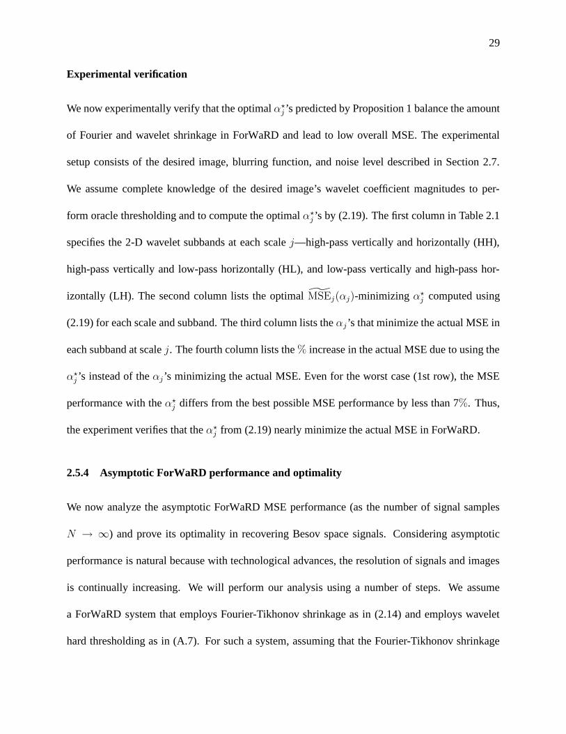
Experimental verification

We now experimentally verify that the optimal α?j ’s predicted by Proposition 1 balance the amount

of Fourier and wavelet shrinkage in ForWaRD and lead to low overall MSE. The experimental

setup consists of the desired image, blurring function, and noise level described in Section 2.7.

We assume complete knowledge of the desired image’s wavelet coefficient magnitudes to per-

form oracle thresholding and to compute the optimal α?j ’s by (2.19). The first column in Table 2.1

specifies the 2-D wavelet subbands at each scale j—high-pass vertically and horizontally (HH),

high-pass vertically and low-pass horizontally (HL), and low-pass vertically and high-pass hor-

izontally (LH). The second column lists the optimal MSEj(αj)-minimizing α?j computed using

(2.19) for each scale and subband. The third column lists the αj’s that minimize the actual MSE in

each subband at scale j. The fourth column lists the % increase in the actual MSE due to using the

α?j ’s instead of the αj’s minimizing the actual MSE. Even for the worst case (1st row), the MSE

performance with the α?j differs from the best possible MSE performance by less than 7%. Thus,

the experiment verifies that the α?j from (2.19) nearly minimize the actual MSE in ForWaRD.

2.5.4 Asymptotic ForWaRD performance and optimality

We now analyze the asymptotic ForWaRD MSE performance (as the number of signal samples

N → ∞) and prove its optimality in recovering Besov space signals. Considering asymptotic

performance is natural because with technological advances, the resolution of signals and images

is continually increasing. We will perform our analysis using a number of steps. We assume

a ForWaRD system that employs Fourier-Tikhonov shrinkage as in (2.14) and employs wavelet

hard thresholding as in (A.7). For such a system, assuming that the Fourier-Tikhonov shrinkage

30

Table 2.1: Experimental verification that (2.19) balances Fourier and wavelet shrinkage inForWaRD.

{j, subband} α?j : MSEj(αj) MSEj(αj) % Increase in

minimizer from (2.19) minimizer MSEj(αj)

{5, HH} 0.16 0.060 6.5{5, HL} 0.16 0.14 0.47{5, LH} 0.23 0.16 0.47{4, HH} 0.18 0.16 0.57{4, HL} 0.29 0.35 0.23{4, LH} 0.34 0.35 0.12{3, HH} 0.33 0.55 5.4{3, HL} 0.50 0.65 6.2{3, LH} 0.55 0.75 6.0{2, HH} 0.84 0.75 1.0{2, HL} 0.95 1.0 0.011{2, LH} 0.93 0.65 2.0{1, HH} 0.98 0.55 3.2{1, HL} 1.0 1.0 0.0{1, LH} 1.0 1.0 0.0

remains unchanged with N and assuming mild conditions on H, we first establish in Proposition

2 the behavior of the distortion due to Fourier shrinkage and the error due to wavelet shrinkage as

N → ∞. Then, in Proposition 3, by allowing the Fourier-Tikhonov shrinkage to decay with N ,

we prove that for scale-invariant deconvolution problems, ForWaRD also enjoys the optimal rate

of MSE decay like the WVD.

Proposition 2 For a ForWaRD system with Fourier-Tikhonov shrinkage λf as in (2.14) with a

fixed τ > 0 and wavelet hard thresholding λw as in (A.7), the per-sample distortion due to loss of

signal components during Fourier shrinkage

1

N

N−1∑

n=0

|x(n)− xλf (n)|2 → C1 (2.20)

31

103

104

105

0.0031

0.0063

0.0125

0.025

0.05

number of samples N

MS

E

WVD: total MSEForWaRD: total MSEForWaRD: wavelet shrinkage errorForWaRD: Fourier distortion error

Figure 2.6: MSE performance of ForWaRD compared to the WVD [8] at different N . The MSEincurred by ForWaRD’s wavelet shrinkage step decays much faster than the WVD’s MSE withincreasing N , while the Fourier distortion error saturates to a constant.

as N → ∞, with C1 > 0 a constant. Further, if the underlying continuous-time x(t) ∈ Bsp,q,

s > 1p− 1

2, 1 < p, q < ∞ and H is a convolution operator whose squared-magnitude frequency

response is of bounded variation over dyadic frequency intervals, then the per-sample wavelet

shrinkage error in estimating the signal part xλf retained during Fourier shrinkage with λf decays

with N →∞ as

1

NE

(N−1∑

n=0

|xλf (n)− x(n)|2)≤ C2N

−2s2s+1 (2.21)

with C2 > 0 a constant and x the ForWaRD estimate.

Refer to Appendix D for the proof of (2.21); the proof of (2.20) is immediate. The bounded

variation assumption is a mild smoothness requirement that is satisfied by a wide variety of H.

The bound (2.21) in Proposition 2 asserts that ForWaRD’s wavelet shrinkage step is extremely

effective, but it comes at the cost of a constant per-sample distortion (assuming τ is kept constant

with N ).

32

10 15 20 25 30 35

0.0016

0.0031

0.0063

0.0125

0.025

0.05

BSNR (dB)

MS

E

Mirror: total MSEForWaRD: total MSEForWaRD: wavelet shrinkage errorForWaRD: Fourier distortion error

Figure 2.7: MSE performance of ForWaRD compared to the mirror-wavelet basis approach [5] atdifferent BSNRs.

Consider an example usingH with frequency response |H(fk)| ∝ (|k|+1)−ν, ν > 0, for which

the WVD is optimal. The per-sample ForWaRD MSE (assuming constant τ > 0 with N ) decays

with a rapid rate of N−2s2s+1 but converges to a non-zero constant. In contrast, the per-sample WVD

MSE decays to zero but with a slower rate of N−2s

2s+2ν+1 (see (2.15)) [8]. Thus, the drawback of

the asymptotic bias is offset by the much improved ForWaRD MSE performance at small sample

lengths. To experimentally verify ForWaRD’s asymptotic performance and compare it with WVD,

we blurred the 1-D, zero-mean Blocks test signal (see Fig. 2.5(a) (top)) using H with a DFT re-

sponse H(fk) = 200/(|k|+ 1)−2 and added noise with variance σ2 = 0.01 for N ranging from 29

to 218. To obtain the ForWaRD estimate, we employ Fourier-Tikhonov shrinkage using (2.14) with

τ = 5 × 10−4. For both the ForWaRD and WVD estimate, we employ wavelet shrinkage using

(A.7) with ρj =√

2 logN [10, 27]. Figure 2.6(a) verifies that ForWaRD’s Fourier distortion error

stays unchanged with N ; the smaller the Fourier shrinkage (smaller τ ), the smaller the distortion.

However, ForWaRD’s wavelet shrinkage error decays significantly faster with increasing N than

the overall WVD error. Consequently, the overall ForWaRD MSE remains below the WVD MSE

33

over a wide range of sample lengths N that are of practical interest.

If τ is kept fixed with increasing N , then the WVD MSE will eventually catch up and improve

upon the ForWaRD MSE. We will now show that if the τ controlling the Fourier shrinkage in

ForWaRD is tuned appropriately at each N , then as stated in Proposition 3, ForWaRD will also

enjoy an asymptotically optimal MSE decay rate like the WVD.

Proposition 3 Let H be an operator with frequency response |H(fk)| ∝ (|k| + 1)−ν, ν > 0. Let

x(t) ∈ Bsp,q, s > min

(0,(

2p− 1)ν, 1

p− 1

2

), 1 < p, q < ∞. Consider a ForWaRD system with

Fourier-Tikhonov shrinkage λf as in (2.14) and wavelet hard thresholding λw as in (A.7). If the τ

parameterizing λf is such that

τ ≤ C3N−β, (2.22)

with

β >s

2s+ 2ν + 1max

1,

4ν

min(2s, 2s+ 1− 2

p

)

, (2.23)

for some constant C3 > 0, then the per-sample ForWaRD MSE decays as

1

NE

(N−1∑

n=0

|x(n)− x(n)|2)≤ C4N

−2s2s+2ν+1 (2.24)

with N → ∞ for some constant C4 > 0. Further, no estimator can achieve a faster error decay

rate than ForWaRD for every x(t) ∈ Bsp,q.

The basic idea behind the proof is to show that both the wavelet shrinkage error (2.21) and the

Fourier distortion error (2.20) decay as N−2s

2s+2ν+1 (see Appendix E for the details). It is easy to

infer that the wavelet shrinkage error decays as fast as the WVD error due to the relatively lower

34

noise levels after Fourier shrinkage. The Fourier distortion error monotonically increases with τ .

We prove that a τ that decays as N−β drives the Fourier distortion error to also decay as N−2s

2s+2ν+1 .

For example, Proposition 3 guarantees that if x(t) ∈ B11,1, ν = 0.5, and τ ∝ N−β at each N with

β > 0.5, then the per-sample ForWaRD MSE will decay at the optimal rate of N−2

7 as N →∞.

Further, tuning τ to precisely minimize the ForWaRD MSE at each N would ensure that the

ForWaRD MSE curve remains below (or at least matches) the WVD’s MSE curve at all sample

lengths for scale-invariant H. This follows from the fact that for τ = 0, ForWaRD is trivially

equivalent to the WVD.

ForWaRD can also match or improve upon the performance of adapted mirror-wavelet decon-

volution [5]. To experimentally compare the MSE performance of ForWaRD with mirror-wavelets,

we blurred the 1-D, zero-mean Blocks test signal (see Fig. 2.5(a) (top)) using H with a DFT re-

sponse H(fk) = (1− 2|k|N

)2. The mirror-wavelet approach is designed to optimally tackle such a

hyperbolic deconvolution problem [5]. We fixed the number of samples at N = 1024 and varied

the amount of additive noise so that the blurred signal-to-noise ratios (BSNRs) ranged from 10 dB

to 35 dB. The BSNR is defined as 10 log10

(‖(x

�h)−µ(x

�h)‖22

Nσ2

), where µ(x~h) denotes the mean of

the blurred image x ~ h samples. To obtain the ForWaRD estimate at each BSNR, we employed

Fourier-Tikhonov shrinkage using τ = 10−2. In the wavelet and mirror-wavelet domain, we em-

ployed shrinkage using (A.7) with ρj =√

2 logN to obtain the ForWaRD and mirror-wavelet

estimate respectively. In Fig. 2.7(b), the MSE incurred by ForWaRD’s wavelet shrinkage step

decays much faster than the mirror-wavelet’s MSE with increasing BSNR (that is, with reducing

noise), while the Fourier distortion error stays constant. The overall ForWaRD MSE stays below

the mirror-wavelet MSE over the entire BSNR range. The ForWaRD performance demonstrated in

35

Fig. 2.7(b) gives us reason to conjecture that ForWaRD with appropriately chosen Fourier shrink-

age should match mirror-wavelet’s optimal asymptotic performance in hyperbolic deconvolution

problems.

2.6 ForWaRD Implementation

To ensure good results with ForWaRD, the noise variance σ2, the Fourier shrinkage, and the

wavelet shrinkage on ForWaRD need to be set appropriately.

2.6.1 Estimation of σ2

The variance σ2 of the additive noise γ in (2.1) is typically unknown in practice and must be

estimated from the observation y. The noise variance can be reliably estimated using a median

estimator on the finest scale wavelet coefficients of y [22].

2.6.2 Choice of Fourier shrinkage

In practice, we employ Fourier-Tikhonov shrinkage λf (see (2.14)) with the parameter τ > 0 set

judiciously. We desire to choose the τ that minimizes the ForWaRD MSE ‖x − x‖22. However,

since x is unknown, we set τ such that the ForWaRD estimate agrees well with the observation y.

That is, we choose the τ that minimizes the observation-based cost

N2∑

k=−N2

+1

|H(fk)|2|H(fk)|2 + η

1

|H(fk)|∣∣∣H(fk)X(fk)− Y (fk)

∣∣∣2

(2.25)

with η := Nσ2

‖y−µ(y)‖22

and µ(y) :=∑

ny(n)N

the mean value of y. The term |H(fk)|2

|H(fk)|2+η(see (2.12)) sim-

ply weighs the error∣∣∣H(fk)X(fk)− Y (fk)

∣∣∣2

between the blurred estimate and the observation at

36

10−6

10−5

10−4

10−3

10−2

50

100

150

200

250

300

350

400

450

500

550

600

regularization τ

Cost (30)MSECost minimizer τMSE minimizer τ

10−5

10−4

10−3

10−2

10−1

50

100

150

200

250

300

350

400

450

500

550

600

regularization τ

Cost (30)MSECost minimizer τMSE minimizer τ

(a) 40 dB BSNR (b) 30 dB BSNRFigure 2.8: Choice of Fourier-Tikhonov regularization parameter τ . In each plot, the solid linedenotes the observation-based cost (2.25) and the dashed lines denotes the actual MSE; the re-spective minima are marked by “◦” and “×”. The plots illustrate that the cost (2.25)-minimizingτ ’s at 40 dB and 30 dB BSNRs yield estimates whose MSEs are within 0.1 dB of the minimumpossible MSE.

the different frequencies to appropriately counter-balance the effect of 1H(fk)

. The τ that minimizes

the cost (2.25) provides near-optimal MSE results for a wide variety of signals and convolution

operators. For example, for the problem setup described in Section 2.7 with 40 dB and 30 dB

BSNRs, Fig. 2.8(a) and (b) illustrate that the τ ’s minimizing (2.25) yield estimates whose MSEs

are within 0.1 dB of the minimum possible MSEs. Since the MSE performance of ForWaRD is

insensitive to small changes around the MSE-optimal τ , a logarithmically spaced sampling of the

typically observed τ -range [0.01, 10]× N σ2

‖y−µ(y)‖22

is sufficient to efficiently estimate the best τ and

determine the Fourier shrinkage λf .

2.6.3 Choice of wavelet basis and shrinkage

Estimates obtained by shrinking DWT coefficients are not shift-invariant, that is, translations of

y will result in different ForWaRD estimates. We exploit the redundant, shift-invariant DWT to

37

obtain improved shift-invariant estimates [10] by averaging over all possible shifts at O(N logN)

computational cost for N -sample signals. (Complex wavelets can also be employed to obtain

near shift-invariant estimates at reduced computational cost [29, 30]). We shrink the redundant

DWT coefficients using the WWF (see (A.8)) rather than hard thresholding due to its superior

performance.

2.7 Results

2.7.1 Simulated problem

We illustrate the performance of ForWaRD (implemented as described in Section 2.6) using a 2-D

deconvolution problem described by Banham et al. [15]. A self-contained Matlab implementation

of ForWaRD is available at www.dsp.rice.edu/software to facilitate easy reproduction of the results.

We choose the 256× 256 Cameraman image as the x and the 2-D 9×9-point box-car blur H with

discrete-time system response h(n1, n2) = 181

for 0 ≤ n1, n2 ≤ 8 and 0 otherwise. We set the

additive noise variance σ2 such that the BSNR is 40 dB.

Figure 2.4 illustrates the desired x, the observed y, the LTI Wiener filter estimate, and the

ForWaRD estimate. The regularization τ = 3.4× 10−4 determining the Fourier-Tikhonov shrink-

age is computed as described in Section 2.6.2. The |X(fk)|2 required by the LTI Wiener filter

is estimated using the iterative technique of [6]. As we see in Fig. 2.4, the ForWaRD estimate,

with signal-to-noise ratio (SNR) = 22.5 dB, clearly improves upon the LTI Wiener filter estimate,

with SNR = 20.8 dB; the smooth regions and most edges are well-preserved in the ForWaRD es-

timate. In contrast, the LTI Wiener filter estimate displays visually annoying ripples because the

underlying Fourier basis elements have support over the entire spatial domain. The ForWaRD es-

38

timate also improves on the multiscale Kalman estimate proposed by Banham et al. [15] in terms

of improvement in signal-to-noise-ratio (ISNR) := 10 log10(‖x− y‖22/‖x− x‖2

2). (During ISNR

calculations, the y is aligned with the estimate x by undoing the shift caused by the convolution

operator. For the 9×9 box-car operator, y is cyclically shifted by coordinates (4, 4) toward the top-

left corner to the minimize the ISNR [19].) Banham et al. report an ISNR of 6.7 dB; ForWaRD

provides an ISNR of 7.3 dB. For the same experimental setup but with a substantially higher noise

level of BSNR = 30 dB, ForWaRD provides an estimate with SNR = 20.3 dB and ISNR = 5.1 dB

compared to the LTI Wiener filter estimate’s SNR = 19 dB and ISNR = 3.8 dB. Both the WVD and

mirror-wavelet basis approaches [5] are not applicable in these cases since the box-car blur used in

the example has multiple frequency-domain zeros. Wiener SNR = 18.1 dB and ISNR = 3 dB

2.7.2 Real-life application: Magnetic Force Microscopy

We employ ForWaRD on experimental data obtained using Magnetic Force Microscopy (MFM) to

illustrate that it provides good performance on real-life problems as well.5 Figure 2.9(a) shows a

measured MFM image of the surface of a magnetic disk; the tracks of black and white patches are

measured magnetic equivalents of bits 0 and 1. Due to instrument limitations, the MFM observa-

tion in Fig. 2.9(a) is blurred and noisy. The MFM measurement can modeled as being comprised

of a desired image blurred by the sensitivity field function of Fig. 2.9(b) and additive, possibly

colored, noise. Figure 2.9(c) illustrates the ForWaRD estimate obtained assuming that the additive

noise is white; the implementation is described in Section 2.6. The Fig. 2.9(d) estimate is obtained

using a modified ForWaRD implementation that does not assume any knowledge about the noise

5The Magnetic Force Microscopy image and sensitivity field function were provided courtesy ofDr. Frank M. Candocia and Dr. Sakhrat Khizroev from Florida International University, Department of Electrical andComputer Engineering.

39

spectrum. The modified algorithm estimates the additive noise’s variance at each wavelet scale

using a median estimator [22]; in contrast, for the white noise case, a common noise variance is es-

timated for all wavelet scales (see Section 2.6.1). We believe that both Figs. 2.9(c) and (d) provide

fairly accurate and consistent representations of the three bit-tracks in the magnetic disk. However,

the estimates of the background media differ significantly depending on the assumptions about the

additive colored noise’s structure.

40

5

10

15

20

5

10

15

20

0.005

0.01

0.015

0.02

(a) MFM measurement (b) Sensitivity field function

(c) ForWaRD estimate (white noise) (d) ForWaRD estimate (colored noise)

Figure 2.9: (a) Blurred and noisy Magnetic Force Microscopy (MFM) measurement (512 × 512samples). (b) Sensitivity field function. The MFM observation in (a) is believed to have beenblurred by this function. (c) and (d) ForWaRD estimates obtained assuming that the MFM mea-surement contains additive white noise and additive colored colored respectively. Data courtesy ofDr. Frank M. Candocia and Dr. Sakhrat Khizroev from Florida International University, Depart-ment of Electrical and Computer Engineering.

41

Chapter 3

WInHD: Wavelet-based Inverse Halftoning via Deconvolution

Once you become informed, you start seeing complexities and shades of gray.

You realize that nothing is as clear and simple as it first appears.

–Bill Watterson

3.1 Introduction

Digital halftoning is a common technique used to render a sampled gray-scale image using only

black or white dots [1] (see Figures 3.3(a) and (b)); the rendered bi-level image is referred to as a

halftone. Inverse halftoning is the process of retrieving a gray-scale image from a given halftone.

Applications of inverse halftoning include rehalftoning, halftone resizing, halftone tone correction,

and facsimile image compression [2, 31]. In this chapter, we focus on inverse halftoning images

that are halftoned using popular error diffusion techniques such as those of Floyd et al. [32], and

Jarvis et al. [33] (hereby referred to as Floyd and Jarvis respectively).

Error-diffused halftoning is non-linear because it uses a quantizer to generate halftones. Re-

cently, Kite et al. proposed an accurate linear approximation model for error diffusion halftoning

(see Figure 3.4) [34, 35]. Under this model, the halftone y(n1, n2) is expressed in terms of the

42

original gray-scale image x(n1, n2) and additive white noise γ(n1, n2) as (see Figure 3.1)

y(n1, n2) = Px(n1, n2) +Qγ(n1, n2)

= (p ∗ x)(n1, n2) + (q ∗ γ)(n1, n2), (3.1)

with ∗ denoting convolution and (n1, n2) indexing the pixels. The P and Q are the linear time-

invariant (LTI) systems with respective impulse responses p(n1, n2) and q(n1, n2) determined by

the error diffusion technique.

From (3.1), we infer that inverse halftoning can be posed as the classical deconvolution problem

because the gray-scale image x(n1, n2) can be obtained from the halftone y(n1, n2) by deconvolv-

ing the filter P in the presence of the colored noise Qγ(n1, n2). Conventionally, deconvolution is

performed in the Fourier domain. The Wiener deconvolution filter, for example, would estimate

x(n1, n2) by inverting P and regularizing the resulting noise with scalar Fourier shrinkage. As we

will see, inverse halftoning using a Gaussian low-pass filter (GLPF) [36] can be interpreted as a

naive Fourier deconvolution approach to inverse halftoning.

Unfortunately, all Fourier-based deconvolution techniques induce ringing and blurring artifacts

due to the fact that the energy of edge discontinuities spreads over many Fourier coefficients.

As a result of this uneconomical representation, the desirable edge Fourier coefficients are easily

confounded with those due to the noise [8, 10, 11].

In contrast, the wavelet transform provides an economical representation for images with sharp

edges [37]. This economy makes edge wavelet coefficients easy to distinguish from those due to

the noise and has led to powerful image estimation algorithms based on scalar wavelet shrinkage

[10, 27].

43

������

-

6

6

--

LTI system

Noise

Gray-scale

x(n1, n2)

Halftone

y(n1, n2)

γ(n1, n2)

LTI system

P

Q

Figure 3.1: Linear approximation for error diffusion halftoning. Under the linear model of [34,35], the error-diffused halftone y(n1, n2) comprises the original gray-scale image x(n1, n2) passedthrough an LTI system P and white noise γ(n1, n2) colored by an LTI system Q. The systems Pand Q are determined by the error diffusion technique.

The wavelet transform was first exploited in inverse halftoning by J. Luo et al. [38]. Xiong et al.

extended this algorithm using non-orthogonal, redundant wavelets to obtain improved results for

error-diffused halftones [39]. Both these algorithms rely on a variety of steps such as clipping and

edge-adapted noise attenuation in the wavelet subbands to exploit different empirical observations.

However, these steps and their implications are not theoretically well-justified.

To simultaneously exploit the economy of wavelet representations and the interplay between

inverse halftoning and deconvolution, we propose the Wavelet-based Inverse Halftoning via De-

convolution (WInHD) algorithm (see Figure 3.2) [40]. WInHD provides robust estimates by first

inverting the convolution operator P determined by the linear model (3.1) for error diffusion and

then effectively attenuating the residual colored noise using wavelet-domain scalar shrinkage oper-

ations [22, 27]. Since WInHD is model-based, it easily adapts to different error diffusion halftoning

techniques. See Figure 3.3 for simulation results.

44

-- -x(n1, n2) WInHD estimate

xλw(n1, n2)P−1

Waveletshrinkage

λw

Halftone

y(n1, n2)

Figure 3.2: Wavelet-based Inverse Halftoning via Deconvolution (WInHD). WInHD inverts theconvolution operator P to obtain a noisy estimate x(n1, n2) of the gray-scale image. Subsequentscalar shrinkage with λw in the wavelet domain (for example, level-dependent hard threshold-ing) effectively attenuates the residual noise corrupting x(n1, n2) to yield the WInHD estimatexλw(n1, n2).

Unlike previous inverse halftoning algorithms, we can analyze the theoretical performance

of WInHD under certain conditions. For images in a Besov smoothness space, we derive the

minimum rate at which the WInHD estimate’s mean-squared-error (MSE) decays as the resolution

increases; that is, as number of pixels in the gray-scale image tends to infinity. We assume that the

linear model for error diffusion (3.1) is exact and that the noise γ(n1, n2) is Gaussian. Further, if

the gray-scale image x(n1, n2) contains some additive noise (say, scanner noise) before halftoning

that is Gaussian, then we show that the MSE decay rate enjoyed by WInHD in estimating the

noise-free x(n1, n2) is optimal; that is, no other inverse halftoning algorithm can have a better

error decay rate for every Besov space image as the number of image pixels increases.

Section 3.2 describes Kite et al.’s linear model for error diffusion halftoning from [34, 35]. Sec-

tion 3.3 clarifies the equivalence between inverse halftoning and deconvolution and also analyzes

Fourier-domain inverse halftoning. Section 3.4 discusses the proposed WInHD algorithm and its

theoretical performance. Section 3.5 illustrates the experimental performance of WInHD. A short

overview of wavelets in Appendix A and a technical proof in Appendix F complement this chapter.

45

(a) Original x(n1, n2) (b) Floyd halftone y(n1, n2)

(c) Gradient estimate [41] (PSNR = 31.3 dB) (d) WInHD estimate (PSNR = 32.1 dB)

Figure 3.3: (a) Original Lena image (512×512 pixels). (b) Floyd halftone. (c) Multiscale gradient-based estimate [41], PSNR = 31.3 dB. (d) WInHD yields competitive PSNR performance (32.1 dB)and visual performance. (All documents including the above images undergo halftoning duringprinting. To minimize the halftoning effect, the images have been reproduced at the maximum sizepossible.) See Figure 3.8 for image close-ups.

46

������

������

Gray-scale

x(n1, n2)

Halftone

y(n1, n2)-

?

- -

�

6

�

Quantizer

H

Error filter

e(n1, n2)-

+

x′(n1, n2)

(a) Error diffusion halftoning

������

������

������Gray-scale

x(n1, n2)

Halftone

y(n1, n2)-

?�

6

�

- - -?

H

Error filter

e(n1, n2)-

+

K

Noise

γ(n1, n2)Gain

x′(n1, n2)

(b) Linear approximation

Figure 3.4: (a) Error diffusion halftoning. The gray-scale image pixels x(n1, n2) are quantized toyield y(n1, n2) and the quantization error e(n1, n2) is diffused over a causal neighborhood by theerror filter H. (b) The linear model approximates the quantizer with gain K and additive whitenoise γ(n1, n2) [34].

3.2 Linear Model for Error Diffusion

In this section, we describe the non-linear error diffusion halftoning and the linear approximation

proposed in [34, 35].

Digital halftoning is a process that converts a given gray-scale digital image (for example, each

pixel value ∈ [0, 1, . . . , 255]) into a bi-level image (for example, each pixel value = 0 or 255) [1].

Error diffusion halftoning is one popular approach to perform digital halftoning. The idea is to take

47

116

x153

7

h(n1, n2) for Floyd [32]

1 x48

5

75

1 3

7

3 5 3

335

h(n1, n2) for Jarvis [33]

Figure 3.5: Error filters h(n1, n2) for Floyd [32] and Jarvis [33] error diffusion. The quantizationerror at the black dot is diffused over a causal neighborhood according the displayed weights.

the error from quantizing a gray-scale pixel to a bi-level pixel and diffuse this quantization error

over a causal neighborhood. The error diffusion ensures that the spatially-localized average pixel

values of the halftone and original gray-scale image are similar; therefore, the halftone visually

resembles the gray-scale image. Figure 3.4(a) illustrates the block diagram for error diffusion

halftoning. The x(n1, n2) denote the pixels of the input gray-scale image and y(n1, n2) denote the

bi-level pixels of the output halftone. The x′(n1, n2), which yields y(n1, n2) after quantization,

is obtained by diffusing the quantization error e(n1, n2) over a causal neighborhood of x(n1, n2)

using the error filter H. The quantizer makes error-diffused halftoning a non-linear technique.

Error diffusion techniques such as Floyd [32] and Jarvis [33] are characterized by their choice of

H’s impulse response h(n1, n2) (see Figure 3.5).

Recently, Kite et al. proposed an accurate linear model for error diffusion halftoning [34, 35].

This model accurately predicts the “blue noise” (high-frequency noise) and edge sharpening effects

observed in various error-diffused halftones. As shown in Figure 3.4(b), this model approximates

the effects of quantization using a gain K followed by the addition of white noise γ(n1, n2). The

48

halftone y(n1, n2) can then be written in terms of the gray-scale image x(n1, n2) and the additive

white noise γ(n1, n2) as in (3.1); the error diffusion technique determines the 2-dimensional (2-D)

frequency responses of the LTI filters P and Q as

P (f1, f2) :=K

1 + (K − 1)H(f1, f2), (3.2)

Q(f1, f2) :=1−H(f1, f2)

1 + (K − 1)H(f1, f2)(3.3)

with P (f1, f2), Q(f1, f2), and H(f1, f2) denoting the respective 2-D Fourier transforms of

p(n1, n2), q(n1, n2), and h(n1, n2). For any given error diffusion technique, Kite et al. found that

the gain K is almost constant for different images. However, the K varied with the error diffusion

technique [34]; for example,K = 2.03 for Floyd, whileK = 4.45 for Jarvis. Figure 3.6 (a) and (b)

illustrate the radially-averaged frequency response magnitudes of the filters P andQ for Floyd and

Jarvis respectively; these responses are obtained by averaging over an annulus of constant radius

in the 2-D frequency domain [1]. In [35], Kite et al. further generalized the linear model of (3.1)

by using different gains Ks and Kn in the signal transfer function P (f1, f2) and the noise trans-

fer function Q(f1, f2) respectively: P (f1, f2) := Ks

1+(Ks−1)H(f1,f2)and Q := 1−H(f1,f2)

1+(Kn−1)H(f1,f2). In

this chapter, we assume a single gain factor K for both the signal and noise transfer functions as

proposed in [34].

3.3 Inverse Halftoning ≈ Deconvolution

Given a halftone y(n1, n2) (see Figure 3.4(a)), inverse halftoning aims to estimate the gray-scale

image x(n1, n2). In the classical deconvolution problem, given the blurred and noisy observation

49

0 0.1 0.2 0.3 0.4 0.5 0.6 0.70

1

2

3

4

5

6

7

8

Normalized radial frequency

Mag

nitu

de

|P(f1,f

2)|

|Q(f1,f

2)|

0 0.1 0.2 0.3 0.4 0.5 0.6 0.70

1

2

3

4

5

6

7

8

Normalized radial frequency

Mag

nitu

de

|P(f1,f

2)|

|Q(f1,f

2)|

(a) Floyd (b) Jarvis

Figure 3.6: Plots (a) and (b) respectively illustrate the radially-averaged frequency response mag-nitudes |P (f1, f2)| (solid line) and |Q(f1, f2)| (dotted line) for Floyd and Jarvis. The high-pass|P (f1, f2)| explains the sharpened edges, while the high-pass |Q(f1, f2)| explains the “blue noise”behavior in the halftones.

y(n1, n2) as in (3.1) with known LTI filters responses p(n1, n2) and q(n1, n2), we seek to esti-

mate x(n1, n2). Thus, under the linear model of [34, 35], inverse halftoning can be posed as a

deconvolution problem.

3.3.1 Deconvolution

Due to the interplay between inverse halftoning and deconvolution, the well-studied deconvolu-

tion literature [4, 7, 13] can be exploited to understand inverse halftoning as well. Deconvolution

algorithms conceptually consist of the following steps:

50

1. Operator inversion

Invert the convolution operator P to obtain a noisy estimate x(n1, n2) of the input signal1

x(n1, n2) := P−1y(n1, n2) = x(n1, n2) + P−1Qγ(n1, n2). (3.4)

2. Transform-domain shrinkage

Attenuate the colored noise P−1Qγ(n1, n2) by expressing x(n1, n2) in terms of a chosen

orthonormal basis {bk}N−1k=0 and shrinking the k-th component with a scalar λk, 0 ≤ λk ≤ 1

[9]

xλ :=∑

k

〈x, bk〉λk bk =∑

k

(〈x, bk〉+ 〈P−1Qγ, bk〉

)λk bk (3.5)

to obtain the deconvolution estimate xλ.

The∑

k〈x, bk〉λk bk in (3.5) denotes the retained part of the signal x(n1, n2) that shrinkage

preserves from (3.4), while∑

k〈P−1Qγ, bk〉λk bk denotes the leaked part of the colored noise

P−1Qγ(n1, n2) that shrinkage fails to attenuate. Clearly, we should set λk ≈ 1 if the variance

σ2k := E(|〈P−1Qγ, bk〉|2) of the k-th colored noise component is small relative to the energy

|〈x, bk〉|2 of the corresponding signal component and set λk ≈ 0 otherwise. The shrinkage by λk

can also be interpreted as a form of regularization for the deconvolution inverse problem [7].

The choice of transform domain to perform the shrinkage in deconvolution (see Step 2 above)

critically influences the MSE of the deconvolution estimate. An important fact is that for a given

transform domain, even with the best possible λk’s, the estimate xλ’s MSE is lower-bounded within

1For non-invertible P , we replace P−1 by its pseudo-inverse and x(n1, n2) by its orthogonal projection onto therange of P in (3.4).

51

a factor of 2 by [8, 10, 11]

∑

k

min(|〈x, bk〉|2, σ2

k

). (3.6)

From (3.6), xλ can have small MSE only when most of the signal energy (=∑

k |〈x, bk〉|2) and

colored noise energy (=∑

k σ2k) is captured by just a few transform-domain coefficients — we term

such a representation economical — and when the energy-capturing coefficients for the signal and

noise are different. Otherwise, the xλ is either excessively noisy due to leaked noise components

or distorted due to lost signal components.

Traditionally, the Fourier domain (with sinusoidal bk) is used to estimate x(n1, n2) from

x(n1, n2) because it represents the colored noise P−1Qγ(n1, n2) in (3.4) most economically. That

is, among orthonormal transforms, the Fourier transform captures the maximum colored noise

energy using a fixed number of coefficients because it diagonalizes convolution operators [26].

Fourier-based deconvolution performs both the operator inversion and the shrinkage simultane-

ously in the Fourier domain as

Xλf := Y (f1, f2)1

P (f1, f2)λf

f1,f2(3.7)

with shrinkage

λff1,f2

:=|P (f1, f2)|2

|P (f1, f2)|2 + Υ(f1, f2)|Q(f1, f2)|2(3.8)

at the different frequencies. The Y (f1, f2) and Xλf (f1, f2) denote the 2-D Fourier transforms of

y(n1, n2) and the deconvolution estimate xλf (n1, n2) respectively. The Υ(f1, f2) in (3.8) is called

the regularization term and is set appropriately during deconvolution [7]. For example, using the

signal to noise ratio to set Υ(f1, f2) =�(|Γ(f1 ,f2)|2)|X(f1,f2)|2

in (3.7) yields the Wiener deconvolution esti-

52

mate [25]; the Γ(f1, f2) and X(f1, f2) denote the respective Fourier transforms of γ(n1, n2) and

x(n1, n2). The 1P (f1,f2)

λff1,f2

in (3.7) constitutes the frequency response of the so-called deconvo-

lution filter.

Fourier-based deconvolution suffers from the drawback that its estimates for images with sharp

edges are unsatisfactory either due to excessive noise or due to distortions such as blurring or ring-

ing. Since the energy due to the edge discontinuities spreads over many image Fourier coefficients,

as dictated by the MSE bound in (3.6), any estimate obtained via Fourier-domain shrinkage suffers

from a large MSE.

3.3.2 Inverse halftoning via Gaussian low-pass filtering (GLPF)

Conventionally, inverse halftoning has been performed using a finite impulse response (FIR) Gaus-

sian filter with coefficients g(n1, n2) ∝ exp[−(n21 + n2

2)/(2σ2g)], where −4 ≤ n1, n2 ≤ 4, and σg

determines the bandwidth [36]. We can interpret inverse halftoning using GLPF as a naive Fourier-

domain deconvolution approach to inverse halftoning. This is substantiated by our observation that

the deconvolution filter 1P (f1,f2)

λff1,f2

(see (3.7) and (3.8)) constructed with the linear model fil-

ters P and Q for Floyd and with regularization Υ(f1, f2) ∝ 1f21+f2

2

has a frequency response that

closely matches the frequency response of the GLPF (see Figure 3.7) [36]. The corresponding

inverse halftone estimates obtained using simulations are also nearly identical. Predictably, GLPF

estimates suffer from the same drawbacks that afflict any Fourier-based deconvolution estimate —

excessive noise (when σg is small) or significant blurring (when σg is large). Exploiting the insights

provided by the deconvolution perspective, we can infer that unsatisfactory GLPF estimates result

because the Fourier domain does not economically represent images with edges.

53

0 0.1 0.2 0.3 0.4 0.5 0.6 0.7

10−4

10−3

10−2

10−1

100

Normalized radial frequency

Mag

nitu

de

Fourier deconvolutionGaussian LPF

Figure 3.7: Comparison of radially-averaged frequency response magnitudes of the FIR GLPF(dashed line) used for inverse halftoning in [36] with the response of the deconvolution filter (solidline) constructed with filters P and Q for Floyd and with Υ(f1, f2) ∝ 1

f21+f2

2

(see (3.7) and (3.8)).Ripples in the GLPF frequency response result because the filter is truncated in space.

3.4 Wavelet-based Inverse Halftoning Via Deconvolution (WInHD)

To simultaneously exploit the economy of wavelet representations (refer Appendix A for an

overview of wavelets) and our realization about the interplay between inverse halftoning and de-

convolution, we propose the WInHD algorithm [40]. WInHD adopts the wavelet-based deconvo-

lution approach of [8] to perform inverse halftoning.

3.4.1 WInHD algorithm

WInHD employs scalar shrinkage in the wavelet domain to perform inverse halftoning as follows

(see Figure 3.2):.

1. Operator inversion

As in (3.4), obtain a noisy estimate x(n1, n2) of the input image by inverting P .

54

2. Wavelet-domain shrinkage

Employ scalar shrinkage in the wavelet domain to attenuate the noise P−1Qγ(n1, n2) in

x(n1, n2) and obtain the WInHD estimate xλw(n1, n2) as follows:

(a) Compute the DWT of the noisy x to obtain wj,` := 〈x , ψj,`〉.

(b) Shrink the noisy wj,` with scalars λwj,` (using (A.7) or (A.8)) to obtain wj,`;λw :=

wj,` λwj,`. The colored noise variance at each scale j determining the λw

j,` is given by

σ2j := E

(|〈P−1Q γ , ψj,`〉|2

).

(c) Compute the inverse DWT with the shrunk wj,`;λw to obtain the WInHD estimate

xλw(n1, n2).

For error diffusion systems, P−1 is an FIR filter. Hence, the noisy estimate x(n1, n2) obtained

in Step 1 using P−1 is well-defined. The subsequent wavelet-domain shrinkage in Step 2 effec-

tively extracts the few dominant wavelet components of the desired gray-scale image x(n1, n2)

from the noisy x(n1, n2) because the residual noise P−1Q γ(n1, n2) corrupting the wavelet com-

ponents is not excessive.

WInHD can be easily adapted to different error diffusion techniques simply by choosing the

gain K recommended by [34] and the error filter response h(n1, n2) for the target error diffusion

technique. K and h(n1, n2) determine the filters P andQ (see (3.2) and (3.3)) required to perform

WInHD. In contrast, the gradient-based inverse halftoning method [41] adapts to a given error

diffusion technique by employing a set of smoothing filters that need to be designed carefully.

55

3.4.2 Asymptotic performance of WInHD

With advances in technology, the spatial resolution of digital images (controlled by the number of

pixels N ) has been steadily increasing. Hence any inverse halftoning algorithm should not only

perform well at a fixed resolution but should also guarantee good performances at higher spatial

resolutions. In this section, under some assumed conditions, we deduce the rate at which the

per-pixel MSE for WInHD decays as number of pixels N →∞.

Invoking established results in wavelet-based image estimation in Gaussian noise, we prove the

following proposition in Appendix F about the asymptotic performance of WInHD.

Proposition 4 Let x(n1, n2) be aN -pixel gray-scale image obtained as in (A.3) by uniformly sam-

pling a continuous-space image x(t1, t2) ∈ Bsp,q with t1, t2 ∈ [0, 1), s > 2

p− 1, and 1 < p, q, <∞.

Let p(n1, n2) and q(n1, n2) denote known filter impulse responses that are invariant with N and

with Fourier transform magnitudes |P (f1, f2)| ≥ ε > 0 and |Q(f1, f2)| <∞. Let y(n1, n2) be ob-

servations obtained as in (3.1) with γ(n1, n2) zero-mean AWGN samples with variance σ2. Then,

the per-pixel MSE of the WInHD estimate x(n1, n2) obtained from y(n1, n2) using hard threshold-

ing behaves as

1

NE

(∑

n1,n2

|x(n1, n2)− x(n1, n2)|2)≤ C N

−ss+1 , N →∞, (3.9)

with constant C > 0 independent of N .

The above proposition affirms that the per-pixel MSE of the WInHD estimate decays as N−ss+1 with

increasing spatial resolution (N →∞) under the mild assumptions discussed below.

The central assumption in Proposition 4 is that the linear model (3.1) for error diffusion

56

is accurate. This is well-substantiated in [34, 35]. The conditions |P (f1, f2)| ≥ ε > 0 and

|Q(f1, f2)| < ∞ respectively ensure that P is invertible and that the variance of the colored noise

Qγ(n1, n2) is bounded. We have verified that for common error diffusion halftoning techniques

such as Floyd and Jarvis, the filters P and Q recommended by the linear model of Kite et al. sat-

isfy these conditions (see Figure 3.6). The final assumption is that the noise γ(n1, n2) is Gaussian;

this is required to invoke the established results on the asymptotics of wavelet-based estimators

[22]. However, recently, wavelet-domain thresholding has been shown to be optimal for many

other noise distributions as well [42, 43]. Hence the noise Gaussianity assumption in Proposition

4 could be relaxed.

Often, gray-scale digital images are corrupted with some noise before being subjected to

halftoning. For example, sensor noise corrupts images captured by charged coupled device (CCD)

based digital cameras. In such cases as well, WInHD can effectively estimate the noise-free gray-

scale image with an MSE decay rate of N−ss+1 as in Proposition 4. Further, WInHD’s MSE decay

rate can be shown to be optimal. The noise-free gray-scale image and resulting halftone can be

related using the linear model of [34, 35] as

y(n1, n2) = P [x(n1, n2) + β(n1, n2)] +Qγ(n1, n2), (3.10)

with β(n1, n2) denoting the noise corrupting the gray-scale image before halftoning. If the

β(n1, n2) is AWGN with non-zero variance, then we can easily infer that the residual noise after

inverting P in Step 1 of WInHD can be analyzed like white noise because its variance is bounded

but non-zero [8]. Hence we can invoke well-established results on the performance of wavelet-

based signal estimation in the presence of white noise [22, 23, 44] to conclude that no estimator

57

(a) Floyd halftone (b) Gradient estimate (c) WInHD estimate

Figure 3.8: Close-ups (128 × 128 pixels) of (a) Floyd halftone, (b) Gradient estimate [41], and(c) WInHD estimate.

can achieve a better error decay rate than WInHD for every Besov space image. Thus, WInHD is

an optimal estimator for inverse halftoning error-diffused halftones of noisy images.

3.5 Results

We illustrate WInHD’s performance using 512×512-pixel Lena and Peppers test images halftoned

using the Floyd algorithm [32] (see Figure 3.3 and 3.8). All WInHD estimates and software are

available at www.dsp.rice.edu/software. We set the gain K = 2.03, as calculated for

Floyd in [34, 35], and use the Floyd error filter response h(n1, n2) (see Figure 3.5) to characterize

the impulse responses p(n1, n2) and q(n1, n2). Inverting the operator P (Step 2) requires O(N)

operations and memory for a N -pixel image since P−1 is FIR. To perform the wavelet-domain

shrinkage (Step 2), we choose the WWF because it yields better estimates compared to schemes

such as hard thresholding.

Estimates obtained by shrinking DWT coefficients are not shift-invariant; that is, translations

58

of y(n1, n2) will result in different estimates. Hence, we exploit the complex wavelet transform

(CWT) instead of the usual DWT to perform the WWF. The CWT expands images in terms of

shifted and dilated versions of complex-valued basis functions instead of the real-valued basis

functions used by the DWT [29, 30]; the expansion coefficients are also complex-valued. Wavelet-

domain shrinkage using WWF on the CWT coefficient magnitudes yields significantly improved

near shift-invariant estimates with just O(N) operations and memory. (The redundant, shift-

invariant DWT can also be used instead of the CWT to obtain shift-invariant estimates [10], but

the resulting WInHD algorithm requires O(N logN) operations and memory.) The standard de-

viation of the noise γ(n1, n2), which is required during wavelet shrinkage, is calculated using the

standard deviation of y(n1, n2)’s finest scale CWT coefficients.

Figures 3.3 and 3.8 compares the WInHD estimate with the multiscale gradient-based estimate

[41] for the Lena image. We quantify the WInHD’s performance by measuring the peak signal-to-

noise ratio PSNR := 20 log10512×255‖

�

x−x‖2(for 512×512-pixel images with gray levels∈ [0, 1, . . . , 255])

with x(n1, n2) the estimate. Table 3.1 summarizes the PSNR performance and computational

complexity of WInHD compared to published results for inverse halftoning with Gaussian filtering

[36], kernel estimation [31], gradient estimation [41], and wavelet denoising with edge-detection

[39]. We can see that WInHD is competitive with the best published results.

The WInHD estimate yields competitive visual performance as well. We quantify visual per-

formance using two metrics: weighted SNR (WSNR) [45, 46] and the Universal Image Quality

Index (UIQI) [47]. Both metrics were computed using the halftoning toolbox of [48]. The WSNR

is obtained by weighting the SNR in the frequency domain according to a linear model of the hu-

man visual system [45, 46]. The WSNR numbers in Table 3.2 are calculated at a spatial Nyquist

59

Table 3.1: PSNR and computational complexity of inverse halftoning algorithms (N pixels).

Inverse halftoning PSNR (dB) Computationalalgorithm Lena Peppers complexity

Gaussian [36] 28.6 27.6 O(N)Kernel [31] 32.0 30.2 O(N)

Gradient [41] 31.3 31.4 O(N)Wavelet denoising [39] 31.7 30.7 O(N logN)

WInHD 32.1 31.2 O(N)

Table 3.2: Visual metrics for inverse halftoned estimates of Lena.

Algorithm WSNR (dB) UIQIGradient [41] 34.0 0.62

WInHD 35.9 0.62

frequency of 60 cycles/degree. The recently proposed UIQI metric of Wang et al. effectively mod-

els image distortion with a combination of correlation loss, luminance distortion, and contrast

distortion [47]; UIQI ∈ [−1, 1] with larger values implying better image quality. For the Lena

image, WInHD’s performance in terms of both the visual metrics is competitive with the gradient

estimate’s performance (see Table 3.2).

60

Chapter 4

JPEG Compression History Estimation (CHEst) for ColorImages

We live in a rainbow of chaos.

–Paul Cezanne

4.1 Introduction

A digital color image is a collection of pixels, with each pixel typically a 3-dimensional (3-D)

color vector. The vector entries specify the color of the pixel with respect to a chosen color space;

for example, RGB, YCbCr, et cetera. JPEG is a commonly used standard to compress digital color

images [3]. It achieves compression by quantizing the discrete cosine transform (DCT) coefficients

of the image’s three color planes; see Fig. 4.1 for an overview of JPEG. However, the various

settings used during JPEG compression and decompression are not standardized [3]. The following

JPEG settings can be chosen by the user such as an imaging device: (1) the color space used to

independently compress the image’s three color planes; (2) the subsampling employed on each

color plane during compression and the complementary interpolation used during decompression;

and (3) the quantization table used to compress each color plane. We refer to the settings used

during JPEG operations as the image’s JPEG compression history.

An image’s compression history is often not directly available from its current representation.

61

For example, JPEG images are often imported into Microsoft Powerpoint or Word documents

using graphics programs such as Microsoft Clip Gallery and then stored internally using an de-

compressed format. JPEG images are also routinely converted to lossless-compression formats

such as bitmap (BMP) format (say, to create a background image for Windows or to feed a printing

driver) or Tagged Image File Format (TIFF). In such cases, the JPEG compression settings are

discarded after decompression.

The compression history, if available, can be used for a variety of applications. A BMP or

TIFF image’s file-size is significantly larger than the previous JPEG file. The JPEG compression

history enables us to effectively recompress such BMP and TIFF images; JPEG-compressing the

image with previous JPEG settings yields significant file-size reduction without introducing any

additional distortion. The JPEG compression history can also be used by “smart” print servers to

reduce artifacts, such as blocking due to previous JPEG compression, from received BMP images.

To alleviate such artifacts by adapting techniques described in [49–55], the print server would need

the image’s JPEG compression history. An image’s JPEG compression history can also potentially

be used as an authentication feature, for covert messaging, or to uncover the compression settings

used inside digital cameras. Hence, the problem of Compression History Estimation (CHEst) is

useful.

The CHEst problem is relatively unexplored. Fan and de Queiroz have proposed a statistical

framework to perform CHEst for gray-scale images [56]; for a gray-scale image, the compression

history comprises only the quantization table employed during previous JPEG operations. How-

ever, CHEst for color images remains unsolved. In this chapter, we propose new frameworks to

perform CHEst for color images.

62

We first derive a statistical framework to perform CHEst. We realize that due to JPEG’s quan-

tization operation, the DCT coefficient histograms of previously JPEG-compressed images exhibit

near-periodic structure. We statistically characterize this near-periodicity for a single color plane.

The resulting framework can be exploited to estimate a gray-scale image’s compression history,

namely, its quantization table. We extend the statistical framework to color images and design a

dictionary-based CHEst algorithm that provides the maximum a priori (MAP) estimate of a color

image’s compression history

{G, S, Q

}= arg max

G,S,QP (Image, G, S,Q) , (4.1)

with G, S, Q denoting the estimated compression color space, the subsampling and associated

interpolation, and the quantization tables.

For the case when the transform from the color space used by JPEG to perform quantization

to the color space of the image’s current representation is affine and when no subsampling is em-

ployed during JPEG compression, we develop a novel, blind, lattice-based CHEst algorithm. In

this case, we make a fundamental observation that the DCT coefficients of the observed image

closely conform to a 3-D parallelepiped lattice structure determined by the affine color transform.

During our quest to exploit the inherent lattice structure, we discover a fundamentally new con-

tribution to the theory of lattices. We derive the geometric conditions under which a set of lattice

basis vectors contains the shortest non-zero lattice vector. Further, we also discover conditions to

characterize the uniqueness of such basis vector sets. By exploiting our new-found insights and

via novel applications of existing lattice algorithms, we estimate the color image’s compression

history, namely, the affine color transform and the quantization tables.

63

Our proposed CHEst algorithms demonstrate excellent performance in practice. Further, we

verify that CHEst allows us to recompress an image with minimal distortion (large signal-to-noise-

ratio (SNR)) and simultaneously achieve a small file-size.

The rest of this chapter is organized as follows. We first provide a brief overview of color

transforms and JPEG in Sections 4.2 and 4.3. We derive the statistical framework for CHEst for

gray-scale images in Section 4.4 and extend this framework to design a dictionary-based CHEst

algorithm for color images in Section 4.5. In Section 4.6, we present our new contributions to the

theory of lattices and then design a lattice-based CHEst algorithm for cases when the compression

color space is related to the current color space by an affine transformation and demonstrate the

algorithm’s estimation performance using simulations. In Section 4.7, we demonstrate the utility

of CHEst in JPEG recompression.

4.2 Color Spaces and Transforms

Color perception is a sensation produced when incident light excites the receptors in the human

retina. Color can be described by specifying the spectral power distribution of the light. Such a

description is highly redundant because the human retina has only three types of receptors that

influence color perception.1 Consequently, three numerical components are sufficient to describe

a color; this is termed the trichromatic theory [57].

Based on the trichromatic theory, digital color imaging devices use three parameters to specify

any color; the three parameters can be viewed as a 3-D vector. The color space is the reference

coordinate system with respect to which the 3-D vector describes color. There exist many different

1A fourth type of receptor is also present in the retina, but it does not affect color perception since it is effectiveonly at extremely low light levels

64

coordinate systems or color spaces according to which a color can be specified. For example,

the Commission Internationale de L’Eclairage (CIE) defined the CIE XYZ color space to specify

all visible colors using positive X, Y, and Z values [57, 58]. Other examples include different

varieties of RGB (Red (R), Green (G), and Blue (B)) and YCbCr (luminance Y, and chrominances

Cb and Cr) color spaces. These color spaces are related to each other and to reference color spaces

such as the CIE XYZ via linear or non-linear color transformations. For example, the popular

Independent JPEG Group (IJG) JPEG implementation [59] converts the 0− 255-valued R, G, and

B components of a digital color image to 0 − 255-valued Y, Cb, and Cr components using the

following transformation

Y

Cb

Cr

=

0.299 0.558 0.114

−0.169 −0.331 0.5

0.5 −0.419 −0.081

R

G

B

+

0

128

128

. (4.2)

The resulting YCbCr space is also referred to as the ITU.BT-601 YCbCr space. The inverse color

transformation from the ITU.BT-601 YCbCr space to the RGB space is given by

R

G

B

=

1.0 0.0 1.40

1.0 −0.344 −0.714

1.0 1.77 0.0

Y

Cb

Cr

−

0

128

128

. (4.3)

The transforms in both (4.2) and (4.3) are affine; we will henceforth refer to the 3× 3 matrix and

the 3× 1 shift (for example, [0 128 128]T in (4.3)) as the affine transform’s linear component and

the additive component respectively.

65

Later in this chapter, we will invoke a variety of color spaces that are inter-related by affine or

non-linear transforms. We refer the reader to [57, 58] for good tutorials on color and for overviews

of the different color spaces and transforms.

4.3 JPEG Overview

DCT

DCT

DCT

IDCT

IDCT

IDCT

to

G

F

transformcolor

subsampling

optionalquantizationcolor space

compressioncolor spaceobservation

Round

Round

Round

round−offinterpolation

F1

F2

F3

G1

G2

G3

compression decompression

Figure 4.1: Overview of JPEG compression and decompression.

In this section, we review JPEG compression and decompression [3]. Consider a color image

that is currently represented in the F color space (see Fig. 4.1); F1, F2, and F3 denote the three

color planes. We refer to the F space as the observation color space. Assume that the image

was previously JPEG-compressed in the G color space—termed compression color space. JPEG

compression performs the following operations independently on each color plane G1, G2, and

G3 in the G space:

1. Optionally downsample each color plane (for example, retain alternate pixels to downsample

by a factor of two); this process is termed subsampling.

2. Split each color plane into 8×8 blocks. Take the DCT of each block.

3. Quantize the DCT coefficients at each frequency to the closest integer multiple of the quan-

tization step-size corresponding to that frequency. For example, if X denotes an arbitrary

66

DCT coefficient and q denote the quantization step-size for the corresponding DCT fre-

quency, then the quantized DCT coefficient X q is obtained by

Xq := round

(X

q

)q. (4.4)

See Fig. 4.2 for examples of quantization tables; each entry in the 8×8 quantization table is

the quantization step-size for an 8×8 image block’s corresponding DCT coefficient.

JPEG decompression performs the following operations:

1. Take the inverse DCTs of the 8×8 blocks of quantized coefficients.

2. Interpolate the downsampled color planes by repetition followed by optional spatial smooth-

ing with a low-pass filter. The popular IJG JPEG implementation [59] uses a 14× [1 2 1]

impulse response filter to smooth in the horizontal and vertical directions.

3. Transform the decompressed image to the desired color space F using the appropriate G to

F transformation.

4. Round-off resulting pixel values to the nearest integer so that they lie in the 0–255 range.

4.4 CHEst for Gray-Scale Images

For gray-scale images, JPEG compression and decompression replicates the steps outlined in Sec-

tion 4.3 for a single color plane but without subsampling and interpolation. Due to JPEG’s quanti-

zation operations, the discrete cosine transform (DCT) coefficient histograms of previously JPEG-

compressed gray-scale images exhibit a near-periodic structure with the period determined by the

67

10 7 6 10 14 24 31 377 7 8 11 16 35 36 338 8 10 14 24 34 41 348 10 13 17 31 52 48 3711 13 22 34 41 65 62 4614 21 33 38 49 62 68 5529 38 47 52 62 73 72 6143 55 57 59 67 60 62 59

10 11 14 28 59 59 59 5911 13 16 40 59 59 59 5914 16 34 59 59 59 59 5928 40 59 59 59 59 59 5959 59 59 59 59 59 59 5959 59 59 59 59 59 59 5959 59 59 59 59 59 59 5959 59 59 59 59 59 59 59

Quantization table 1 Quantization table 2

Figure 4.2: Example of JPEG quantization tables.

quantization step-size. In this section, we derive a statistical framework, which characterizes the

near-periodic structure, to estimate the quantization table.

4.4.1 Statistical framework

An arbitrary DCT coefficient X of a previously JPEG-compressed gray-scale image can be ob-

tained by adding to the corresponding quantized coefficient X q (see (4.4)) a round-off error term

Γ

X = Xq + Γ. (4.5)

As described in [56], we can model Γ using a truncated Gaussian distribution

P (Γ = t) =1

Υexp

(− t2

2σ2

), for t ∈ [−ζ, ζ], (4.6)

with σ2 the variance of the Gaussian, [−ζ, ζ] the support of the truncated Gaussian, and Υ the

normalizing constant. Further, based on studies in [3, 60], we model the DCT coefficients using a

68

zero-mean Laplacian distribution.2

P (X = t) =λ

2exp (−λ|t|) . (4.7)

We have assumed that the parameter λ is known; in practice, we estimate λ from the previously

compressed image for each DCT frequency as described later in this section. From (4.7), we have

Lλ(kq) := P(Xq = kq | q, k ∈ Z

)=

∫ (k+0.5)q

(k−0.5)q

λ

2exp (−λ|τ |) dτ. (4.8)

Hence,

P(Xq = t | q

)=∑

k∈�

δ (t− kq)Lλ(kq). (4.9)

Now, assuming that the round-off error Γ is independent of X and q, the distribution of X is

obtained by convolving the distributions for X and Γ (see Fig. 4.3). That is,

P(X = t | q

)=

∫P(Xq = τ | q

)P (Γ = t− τ) dτ (4.10)

=

∑k∈

� 1Υ

exp(− |t−kq|2

2σ2

)Lλ(kq),

for |t− kq| ∈ [−ζ, ζ],

0, otherwise.

(4.11)

Given a setD of DCT coefficients at a particular frequency that are obtained from a previously

compressed image, we can obtain the MAP estimate q of the quantization step used during previous

2DC components are typically modeled using Gaussian distributions with non-zero mean. To avoid the errorsassociated with estimating the Gaussian’s mean and for simplicity, we assume that the DC coefficient can also bemodeled using a zero-mean Laplacian distribution with zero mean.

69

compression assuming the DCT coefficients are independent as

q = arg maxq∈

�+P (D, q) (4.12)

= arg maxq∈

�+

∏

�

X∈D

P (X | q)P (q)

, (4.13)

where P (q) denotes the prior on q.

4.4.2 Algorithm steps

Based on the statistical framework derived in the previous section, we can estimate the quantization

step-sizes using the following steps:

1. Compute set of the desired frequency DCT coefficients D from the previously compressed

image.

2. Estimate the parameter λ from the observations as

λ =N

∑�

X∈D |X|,

with N the number of coefficients in the set D.

3. Assuming all quantization step-sizes are equally likely, use (4.11) with suitable parameters

σ2 and ζ to estimate

q = arg maxq∈

�+

∏

�

X∈D

P (X | q)

. (4.14)

70

0 10 20 30 40 50 600

50

100

150

Coefficient value

His

togr

am v

alue

Figure 4.3: Histogram of quantized DCT coefficients. The DCT coefficients from DCT frequency (4,4) ofthe gray-scale Lenna image were subjected to quantization with step-size q = 10 during JPEG compressionand then decompressed. Due to roundoff errors, the DCT coefficients are perturbed from integer multiplesof 10.

The above algorithm is a refinement of the technique proposed by Fan and de Queiroz in

[56]. While the core ideas remain the same, the final derived equation (4.11) differs because of

significant variations in the starting points for the derivation and in the intermediate assumptions.

Further, our derivation explicitly accounts for all the normalization constants, thereby allowing us

to extend the above approach to estimate the compression history of color images.

4.5 Dictionary-based CHEst for Color Images

In this section, we build on the quantization step-size estimation algorithm for gray-scale images

to perform CHEst for color images.

4.5.1 Statistical framework

For color images, in addition to quantization, JPEG performs color transformation and subsam-

pling along with the complementary interpolation. We realize that the DCT coefficient histograms

of each color plane exhibit the near-periodic structure of Fig. 4.3 introduced by quantization only

when the image is transformed to the original compression color space and the all interpolation

effects are inverted. Otherwise, the near-periodic structure is not visible. This realization enables

71

us to obtain the MAP estimate of a color image’s compression history as in (4.1) by extending

the statistical framework for gray-scale images a straightforward way. Let DG,S denote the set

of DCT coefficients XG,S obtained by first transforming the image from F to the G color space

representation, then undoing the interpolation S, and finally taking the DCT of the color planes.

Then,

{G, S, Q

}= arg max

G,S,QP (Image|G, S,Q)P (G, S,Q)

= arg maxG,S,Q

P (DG,S|G, S,Q)P (G)P (S)P (Q)

= arg maxG,S,Q

∏�

XG,S∈DG,S

P(XG,S|G, S,Q

)P (G)P (S)P (Q), (4.15)

assuming that the G, S, and Q are independent. In (4.15), the conditional probability

P (XG,S|G, S,Q) of the DCT coefficients is set to (4.11), which is a metric for how well the

image DCT coefficients conform to a near-periodic structure. Hence, if G, S, and Q were ac-

tually employed during the previous JPEG compression, then the histogram of DG,S exhibits near-

periodicity and the associated P (XG,S|G, S,Q) would be large. Consequently, the MAP estimate

would be accurate.

4.5.2 Algorithm steps

Ideally, the MAP estimation of (4.15) would require a search over allG and S. For practical consid-

erations, we constrain our search to a dictionary of commonly employed compression color spaces

and interpolations. The steps of our simple dictionary-based CHEst algorithm are as follows:

1. Transform the observed color image to a test color space G.

72

2. Undo the effects of the test interpolation S. To undo interpolation by simple repetition,

simply downsample the color plane. To undo interpolation by repetition and smoothing, first

deconvolve the smoothing using a simple Tikhonov-regularized deconvolution filter [24],

and then downsample the color plane.

3. Employ the quantization step-size estimation algorithm of Section 4.4 on the coefficients at

each DCT frequency and each color plane.

4. Output the color transform and interpolation yielding the maximum conditional probability

(see (4.15)) along with the associated quantization tables from Step 3.

The computational complexity of the dictionary-based CHEst algorithm is determined by the size

of the image, the number of the test color spaces, and the number of test subsamplings and inter-

polations. We can easily prune the number of test color spaces and interpolations to reduce the

computational complexity by using a small part of the image. The quantization table estimates can

be perfected using the entire image after the color space and interpolation is quickly determined.

4.5.3 Dictionary-based CHEst results

Our dictionary-based CHEst algorithm precisely estimates the compression history of a previously

JPEG-compressed color image. We demonstrate the performance of our algorithm using the 512×

512 Lenna color image [61]. We JPEG-compressed Lenna in the 8-bit CIELab color space using

the sRGB to 8-bit CIELab color transformation [58] and employed 2×2, 1×1, 1×1 subsampling;

that is, the luminance L color plane is not downsampled, while the chrominance planes a and b are

downsampled by a factor of 2 in the horizontal and vertical directions. We employed quantization

table 1 from Fig. 4.2 for the L plane and quantization table 2 for the both the a and b planes. During

73

decompression, the a and b planes are interpolated by first upsampling using repetition and then

smoothing in the horizontal and vertical directions using a 14× [1 2 1] impulse response filter.

To solve the CHEst problem, we tested all color transforms from a dictionary consisting of

RGB to YCbCr, Computer RGB to ITU.BT-601 YCbCr, Studio RGB to ITU.BT-601 YCbCr, RGB

to Kodak PhotoYCC, sRGB to Linear RGB, sRGB to 8-bit CIELab, and sRGB to CMY transforms

[58]. For each transform, we considered subsampling factors 2× 2, 1× 1, 1× 1 (with and without

smoothing during interpolation) and 1× 1, 1× 1, 1× 1.

During the computations of the conditional probabilities (4.15), we assumed that all color trans-

forms and quantization step-sizes are equally likely; that is, P (G) = P (Q) = 1. During our ex-

periments, we set ζ = 6 (see (4.11)). To test if a color plane was subsampled by a factor of 2 and

then smoothed during interpolation, we set the σ2 = 0.8 (see (4.11)) during the quantization table

estimation step. To test if no smoothing is employed during interpolation, we set σ2 = 0.75, and to

test if no subsampling is employed, we reduced the σ2 to 0.5. Further, we set the prior P (S) = 0.55

for the 2×2, 1×1, 1×1 with smoothing, P (S) = 0.35 for the 2×2, 1×1, 1×1 without smoothing,

and P (S) = 0.1 for the 1 × 1, 1 × 1, 1 × 1 subsampling. When larger subsampling factors and

smoothing are employed, the DCT coefficients deviate further from their quantized values result-

ing in relatively lower conditional probabilities. The adapted σ2 and priors P (S) help level this

effect and correctly detect the compression history of the image.

By comparing the logarithms of the conditional probabilities listed in Table 4.1, we precisely

identify that the sRGB to 8-bit CIELab color transformation was employed with 2× 2, 1× 1, 1× 1

subsampling during the previous compression, and smoothing was employed during the decom-

pression; the corresponding conditional probability value (enclosed by a 2 in the table) is the

74

Table 4.1: Conditional probabilities’ logarithms (×106) for different color transforms and interpolations

Color transform 1× 1, 1× 1, 1× 1 2× 2, 1× 1, 1× 1 2× 2, 1× 1, 1× 1(without smoothing) (with smoothing )

RGB to YCbCr −0.88 −0.88 −0.8Computer RGB to YCbCr −0.83 −0.83 −0.75

Studio RGB to YCbCr −0.88 −0.89 −0.81RGB to Kodak YCC −0.79 −0.78 −0.69sRGB to Linear RGB −1.5 −1.9 −1.8

sRGB to 8-bit CIELab −0.73 −0.71 −0.53

sRGB to CMY −1.5 −1.9 −1.8

largest. Our quantization table estimates are given in Fig. 4.4. (see Fig. 4.2 for the actual tables).

An × indicates that the quantization step-size estimation for the corresponding DCT frequency

was not possible because all the DCT coefficients were quantized to zero during compression.

Our quantization step-size estimates, especially at the most important low frequencies, is accu-

rate. The estimates for the a and the b planes suffer from seemingly large errors. For example,

we incur an error of 52 while estimating an entry in the a plane’s quantization table; the actual

quantization step-size was 59 but our algorithm’s estimate was 7. The error is a result of additional

noise (compared to the no subsampling case) introduced by the deconvolution step (algorithm’s

Step 2)), which is necessary to undo the interpolation . However, the estimation error does not

adversely affect applications such as recompression because, in reality, all the DCT coefficients at

the corresponding frequency were set to zero during quantization.

4.6 Blind Lattice-based CHEst for Color Images

The efficacy of dictionary-based CHEst approach is limited by the richness of the color space

dictionary. If an unknown proprietary color space is used to perform the JPEG compression, then

75

10 7 6 10 14 24 31 377 7 8 11 16 35 36 328 8 10 14 24 34 40 338 10 13 17 31 51 47 3511 13 22 34 40 63 × 4414 21 32 37 47 × × 5128 35 44 49 × × × ×× × × × × × × ×

L’s table

10 11 14 28 54 9 × 911 13 15 36 50 9 7 714 15 30 9 9 5 × 726 34 48 × × × 7 ×× × × × × × × ×× × × × × × × ×× × × × × × × ×× × × × × × × ×

10 11 14 26 × 7 × ×11 13 15 35 × × × ×13 15 31 48 × × × ×25 34 × × × × × ×× × × × × × × ×× × × × × × × ×× × × × × × × ×× × × × × × × ×

a’s table b’s table

Figure 4.4: Quantization tables estimates using the dictionary-based CHEst algorithm for the L, aand b color planes. An × indicates that estimation was not possible because all coefficients werequantized to zero.

the dictionary-based approach will fail to detect it. In this section, we develop an approach that

does not need a dictionary of color spaces, and is hence blind, to estimate the compression history

if the transform from the compression color space to the current color space is affine and if no

subsampling is employed during JPEG compression.

Our fundamental observation is that the DCT coefficients of the observed image closely con-

form to a 3-D parallelepiped lattice structure determined by the affine color transform. We discover

some fascinating, new, and relevant properties of lattices during our theoretical study. We rely on

these new insights and novel applications of existing lattice algorithms to exploit the lattice struc-

ture of our problem and estimate the color image’s compression history.

76

For the sake of clarity, we first describe the estimation of the image’s compression history

assuming that no round-off errors are present; that is, assuming that the DCT coefficients exactly

conform to a 3-D parallelepiped lattice. We then adjust the estimate to combat the round-off noise.

4.6.1 Ideal lattice structure of DCT coefficients

In the absence of round-off noise, the 3-D vector of DCT coefficients of an previously JPEG-

compressed color image conform to a regular parallelepiped lattice structure. This inherent struc-

ture is a result of the quantization undergone during previous JPEG compression.

Consider an arbitrary 8× 8 color image block that the DCT acts on during JPEG compression

in the G color space. Let XG1, XG2, and XG3 denote the respective ith frequency DCT coefficients

of theG1, G2, andG3 planes in the chosen 8×8 color image block, and let qi,1, qi,2, and qi,3 denote

the respective quantization step-sizes. JPEG quantizes the DCT coefficients of the each plane inde-

pendently toXqi,1:= round

(XG1

qi,1

)qi,1,Xqi,2

:= round(

XG2

qi,2

)qi,2, andXqi,3

:= round(

XG3

qi,3

)qi,3

respectively. The 3-D vector of quantized DCT coefficients[Xqi,1

Xqi,2Xqi,3

]T, with superscript

T denoting matrix transpose, along with all the other vectors of quantized ith DCT frequency co-

efficients (see Fig. 4.5), lies on a rectangular box lattice (see Fig. 4.6) with edge-lengths equal to

the quantization step-sizes.

When an image with previously quantized DCT coefficients is represented in another color

space F that is related toG by an affine transformation, then the corresponding 3-D vectors of DCT

coefficients in the F space do not lie on a rectangular box lattice, but rather on a parallelepiped3

lattice, assuming that no round-off is performed during JPEG decompression in the G space. The

3A solid with six faces, each of which is a parallelogram.

77

��

��

��

��

��

��

��

��

��

��

��

��

��

��

��

��

��

��

��

��

��

��

��

��

��

��

��

-

� -

-

�

��

�

��

��

���

��

��

�

��

��

���

��

��

�

��

��

���

��

��

�

��

��

���

��

��

�

��

��

���

��

��

�

♣

♥

♥

♣

♥

♣

♥

♣

♥

♥

♣

♣

Block 1’s DCT Block 2’s DCT

G2

G1

G3

Figure 4.5: 3-D vectors from different 8 × 8 blocks. The vertically stacked triplet of boxes, eachwith dotted lines, represent the DCT coefficients of an 8 × 8 image block. The 3-D vectors[♥G1 ♥G2 ♥G3]

T of quantized DCT coefficients from frequency (3, 3) of Block 1 and Block 2 lieon the same rectangular lattice but at possibly different locations. A different rectangular latticecontains the (5, 6) frequency 3-D vectors [♣ ♣ ♣]T of quantized DCT coefficients.

edges of the parallelepiped are determined by the column vectors of the linear component of the

affine color transform from G to F (for example, see (4.3)), which we henceforth denote by T .

(The additive component of the affine color transform only reflects as a shift in the DC frequency

coefficients.) As we shall soon see, the parallelepiped structure of the DCT coefficients can be

exploited to solve the CHEst problem.

78

(a) G space (ideal) (b) F space (ideal)

(c) G space (with round-off) (d) F space (with round-off)

Figure 4.6: Lattice structures in the previously JPEG-compressed color image: (a) Assuminground-off errors are absent, all 3-D vectors of G space’s DCT coefficients from the different 8× 8image blocks but same DCT frequency lie exactly on the vertices of a rectangular lattice. The 3-Dvectors are denoted by small circles. (b) In the F space, the 3-D vectors of DCT coefficients liesexactly on the vertices of a parallelepiped lattice. (c) and (d) Round-off errors slightly perturb the3-D vectors of DCT coefficients in the G and F color spaces from the vertices of the rectangularlattice and parallelepiped lattice respectively.

4.6.2 Lattice algorithms

Lattices are regular arrangements of points in space and their study arises in a number of fields

such as coding theory, number theory, and crystallography. Consider an ordered set of m vectors

{b1, b2, . . . , bm}. The latticeL spanned by these vectors consists of all integral linear combinations

u1b1 + u2b2 + . . .+ umbm, ∀ui ∈ Z. The structure in Figures 4.6(a) and (b) are both examples of

3-D lattices. Any set {b1, b2, . . . , bm} forms a basis for a given L if the following two conditions

79

hold:

1. Every vector in L can be expressed as u1b1 + u2b2 + . . .+ umbm, ui ∈ Z for i = 1, . . . , m.

2. If u1b1 + u2b2 + . . .+ umbm = 0, ui ∈ Z, then ui = 0 for i = 1, . . . , m.

For any given lattice L, there exist many different sets of basis vectors. If B := [b1 b2 . . . bm]

is a matrix whose columns form a basis for a lattice L, then any arbitrary basis vector set can be

expressed as the columns of B U , where U is an integer matrix with determinant equal to ±1.

Properties of nearly orthogonal lattice basis vectors

Later in this section, we will need to understand and exploit the properties of lattice basis vectors

that are nearly orthogonal. This is because the column vectors of an affine color transform’s linear

component, which determine the structure of the parallelepiped lattice in the F space, are typically

nearly orthogonal. We have discovered two new, fundamental properties of such nearly orthogonal

lattice basis vectors.

To formally describe the two properties, we first need to define the following terms:

• Weak θ-orthogonality: We define an ordered set of vectors {b1, b2, . . . , bm} to be weakly

θ-orthogonal if for any i = 2, . . . , m, the angle between bi and any non-zero linear combi-

nation of {b1, . . . , bi−1} lies in the range [θ, π − θ]; that is,

cos−1

|〈bi,

∑i−1j=1 λi bi〉|

‖bi‖2

∥∥∥∑i−1

j=1 λi bi〉∥∥∥

2

≥ θ, for all

∑

j

|λj| > 0, with λj ∈ R. (4.16)

• Strong θ-orthogonality: We define a set of vectors {b1, b2, . . . , bm} to be strongly

θ-orthogonal if all its permutations are weakly θ-orthogonal.

80

Our first observation is that a nearly orthogonal set of basis vectors contains the shortest non-

zero lattice vector.

Proposition 5 Let B := [b1, b2, . . . , bm] be a matrix whose columns form a ordered set of basis

vectors for a lattice L. If the columns of B are weakly(

π3

+ ε)-orthogonal, 0 ≤ ε ≤ π

6, then B’s

shortest column is the shortest non-zero vector in the lattice L; that is,

minj∈1,...,m

‖bj‖2 ≤∥∥∥∥∥

m∑

i=1

uibi

∥∥∥∥∥2

, for allm∑

i=1

|ui| ≥ 1, with ui ∈ Z. (4.17)

Further, if ε > 0, then

minj∈1,...,m

‖bj‖2 <

∥∥∥∥∥

m∑

i=1

uibi

∥∥∥∥∥2

, for allm∑

i=1

|ui| > 1, with ui ∈ Z. (4.18)

Proposition 5’s proof, which is described in Appendix G.1, follows by induction; it is easy to first

verify that the proposition holds for 2-dimensional (2-D) lattices and then extend the proposition

to higher dimensions. An immediate corollary is

Corollary 1 A strongly π3-orthogonal set of basis vectors contains the shortest non-zero lattice

vector.

Proposition 5 and its corollary are significant contributions to the theory of lattices because the

problem of finding the shortest non-zero vector in an arbitrary lattice is believed to be a NP-hard

problem. To the best of our knowledge, Proposition 5 is the first result that can provide a certificate

that a set of vectors contains the shortest non-zero lattice vector.

81

Our second observation describes the conditions under which a lattice contains a unique (mod-

ulo permutations and sign changes) set of nearly orthogonal lattice basis vectors.

Proposition 6 Let B := [b1 b2 . . . bm] be a matrix whose columns form a basis for a lattice L and

are strongly θ-orthogonal. For all i ∈ 1, . . . , m, if

minj∈1,...,m

‖bj‖2 ≤ ‖bi‖2 < minj∈1,...,m

‖bj‖2 η(θ), (4.19)

with

η(θ) =

(√3 sin(θ)− 3| cos(θ)|

4 sin2(θ)− 3

)(4.20)

then any strongly θ-orthogonal set of basis vectors can be obtained by simply permuting and chang-

ing the signs of the B’s columns.

Proposition 6’s proof is described in Appendix G.1. In words, Proposition 6 claims that a nearly

orthogonal set of basis vectors is unique when the lengths of all the basis vectors are nearly equal.

For example, both Fig. 4.7(a) and (b) illustrate 2-D lattices that can be spanned by orthogonal basis

vectors. For the lattice in Fig. 4.7(a), the ratio of the basis vector’s lengths is less than η(

π2

)=√

3.

Hence, there exists only one set (modulo permutations and sign changes) of basis vectors such that

the angle between them is greater than π3. In contrast, the lattice in Fig. 4.7(b) contains many sets

of strongly π3-orthogonal basis vectors.

Lattice reduction

A celebrated lattice problem of interest to us is the so-called lattice reduction problem, which can

be stated as follows: Given a set of vectors bi’s that span a lattice L, find an ordered set of basis

82

90 deg

(0,0)

(1,1.5)

<60 deg

(0,0)

90 deg >60 deg

(1,2)

(a) (b)

Figure 4.7: (a) The vectors comprising the lattice are denoted by filled circles. The lattice contains twoorthogonal basis vectors with lengths 1 and 1.5 respectively. Since 1.5 <

√3, the lattice contains no other

set of basis vectors such that the angle between them is greater than π3 radians (60 degrees). (b) The lattice

contains two orthogonal basis vectors with lengths 1 and 2 respectively. The figure illustrates two sets ofstrongly π

3 -orthogonal basis vectors for the same lattice.

vectors for L such that [62]

1. the basis vectors are nearly orthogonal,

2. the shorter basis vectors appear first in the ordering.

A major breakthrough in the lattice theory area was the discovery of a polynomial time algorithm to

perform lattice reduction by Lenstra, Lenstra, and Lovasz; this algorithm is referred to as the LLL

algorithm henceforth. The LLL algorithm, which can be intuitively understood as an adaptation of

Gram-Schmidt orthogonalization, performs lattice reduction by sequentially processing the vectors

bi’s and performing a combination of very simple operations such as

1. Change the order of the basis vectors.

2. Add to one of the vectors bi an integral multiple of another vector bj . Note that the vectors

resulting from such integral operations still lie on the same lattice.

83

3. Delete any resulting zero vectors.

The LLL algorithm has since proved invaluable in many areas of mathematics and computer sci-

ence, especially in algorithmic number theory and cryptography [62, 63].

Closest vector problem

The closest vector problem (CVP), another famous lattice problem of interest to us, is closely

related to the lattice reduction problem and can be stated as follows: Given a lattice L and an

arbitrary vector v, find the vector on the lattice L that is closest to v. For a comprehensive semi-

tutorial paper on the CVP and algorithms to solve the same, we refer the reader to [64].

4.6.3 LLL provides parallelepiped lattice’s basis vectors

The LLL algorithm, when employed on the 3-D vectors of F space’s AC frequency DCT coef-

ficients (assuming round-off errors are absent), produces a set of nearly orthogonal, norm-sorted

basis vectors for the parallelepiped lattice containing the 3-D vectors. (Since the additive com-

ponent of the affine color transformation causes an unknown shift in the DC coefficients, the DC

coefficients are handled separately.) In fact, during our experiments, we have observed that the set

of basis vectors returned by LLL is always strongly π3-orthogonal; this conforms with the popular

notion that, in practice, the LLL performs significantly better than what is guaranteed theoretically

[62, 63]. Any basis that spans the parallelepiped lattice of 3-D vectors of F space’s ith-frequency

84

DCT coefficients can be written as

Bi :=

T

qi,1 0 0

0 qi,2 0

0 0 qi,3

Ui

(4.21)

=: T Qi Ui (4.22)

The Ui, which is a unit-determinant matrix with integer entries, accounts for the non-uniqueness

of lattice basis vectors.

4.6.4 Estimating scaled linear component of the color transform

The columns of Bi that is returned by the LLL (see (4.22)) after acting on i-th frequency 3-D

vectors are sometimes misaligned with the columns of T Qi, due to a non-identity Ui. In this

subsection, with the help of Propositions 5 and 6, we determine the appropriate Ui’s, and thereby

extract the T Qi’s from the different Bi’s.

Sometimes, the quantization step-sizes for the three components are chosen to be equal, that

is, qi,1 ≈ qi,2 ≈ qi,3, especially if the compression color space G is a member of RGB family.

Further, the columns of typical T ’s are strongly θ-orthogonal, π3≤ θ ≤ 2π

3. Hence, by invoking

Proposition 6, we can infer that T Qi is the only set of π3-orthogonal basis for the lattice. Hence,

in this case, the LLL algorithm directly estimates the columns of T Qi as the LLL-reduced basis

Bi; that is, the Ui is just permutation a matrix.

Often, the quantization step-sizes at the ith frequency are chosen to be different for the three

components of G. For example, if G is a member of Y CbCr family, then the quantization step-

85

size for the luminance component Y is typically chosen to be much smaller than that for the

chrominance components Cb and Cr. In this case, Proposition 5 helps us infer that the first vector

of Bi is the smallest vector in the lattice and that this vector would necessarily be aligned with one

of T ’s columns. The remaining two Bi columns could be misaligned with the columns of T due

to the addition of a small integer multiple of the smallest vector. For example, Ui could be

1 0 1

0 1 0

0 0 1

,

in which case, the third column vector of the Bi would be misaligned with the third column of T Qi

due to the addition of T Qi’s first column. In this case, we can obtain the columns of T Qi for the

different DCT frequencies by comparing the Bi’s across frequencies and estimating the Ui’s.

From (4.22), we can infer that all of the Ui’s satisfy the property that UiB−1i BjU−1

j is a diagonal

matrix. Since a typical T ’s columns are nearly orthonormal, the actual Ui’s add or subtract at most

a unit multiple of the first column (smallest vector) of Bi to the second and third columns of Bi. If

qj,1

qi,16= qj,2

qi,2and qj,1

qi,16= qj,3

qi,3, which is a reasonable assumption in practice,4 then a unique combination

of Ui and Uj ensures that UiB−1i BjU−1

j is a diagonal matrix. Hence, we simply search for the Ui and

Uj , i 6= j, such that UiB−1i BjU−1

j is a diagonal matrix. This yields the columns of Bi U−1i = T Qi

for the different AC frequencies. (If an rough estimate of T is known, then it is straightforward to

search for a Ui that aligns BiU−1i with the columns of T .)

4Typically, different quantization tables are used for the luminance and chrominance components.

86

4.6.5 Estimating the complete color transform and quantization step-sizes

Once we estimate the scaled linear component of the T Qi for the different AC DCT frequencies,

we can extract the color transform T and quantization step-sizes qi,j .

To extract the linear component T of the color transform from T Qi, we need to estimate the

norms of each of the three columns of T . The columns norms of T are the largest numbers such

that the respective column vectors of T Qi are integer multiples of T . Let T (:, k) and (T Qi) (:, k),

k = {1, 2, 3}, denote the kth column vectors of T and T Qi respectively. We set the norms of T ’s

columns as the solution to the following penalized least-squares cost function,

‖T (:, k)‖2 =

arg minκ

∑

i

((‖(T Qi) (:, k)‖2 − κ round

(‖(T Qi) (:, k)‖2

κ

))2

+ β round

(‖(T Qi) (:, k)‖2

κ

)). (4.23)

The first term ensures that the column norms of T Qi conform to integer multiples of the column

norm of T , and the second term ensures that the column norm of T is large; β controls the tradeoff

between the two terms. Thus, we can estimate T from the different T Qi’s.

Once we know the column norm of T , we can estimate the quantization step-sizes for all the

AC DCT frequencies as qi,k =‖(T Qi)(:,k)‖

2

‖T (:,k)‖2

.

With the knowledge of T , we can also estimate the DC frequency quantization step-sizes and

the additive component of the color transform from the DC frequency DCT coefficients. We first

transform the 3-D vectors of F space’s DC coefficients using T −1. This yields the DC frequency

DCT coefficients of the G space but the coefficients are shifted by an unknown amount due to the

87

additive component of the color transform. Due to quantization, the respective 1-D histograms

of coefficients from each component of the obtained T −1-transformed vectors show a similar be-

havior to that illustrated in Fig. 4.3. To estimate the quantization step-size, we first compute the

magnitude of the Discrete Fourier Transform (DFT) of the histogram, which is immune to the un-

known shift. The near-periodic behavior of the populated histogram bins ensures that the frequency

at which the histogram’s DFT magnitude first peaks away from zero frequency corresponds to the

quantization step-size.

The color transform’s additive component’s coefficients can only be such that the histogram of

estimated G space’s DC frequency DCT coefficients is populated at zero. Further, the typical role

of the additive component of the color transform is to ensure that the component values conform

to the 0–255 range after transformation. Hence, we simply choose the additive component’s coef-

ficients to simultaneously ensure both these properties. We clarify that many solutions can satisfy

the above two criteria. However, fortunately, the mis-estimations in the additive component of the

color transform do not affect typical CHEst applications such as recompression and enhancement.

4.6.6 Round-offs perturb ideal geometry

Round-offs employed during JPEG decompression (see Fig. 4.1 and Section 4.3) perturb the DCT

coefficient values. Consequently, the 3-D vectors of DCT coefficients in the G and F color

spaces lie only approximately on the rectangular lattice and parallelepiped lattice respectively (see

Fig. 4.6).

Let V denote the 3-D error vector that captures the perturbation of a 3-D DCT coefficient

vector from the parallelepiped lattice in the F color space due to round-offs. Based on (4.6), we

88

can statistically model the distribution of the norm of the perturbation vector as

P (‖V ‖2 = t) =1

Υexp

(− t2

2σ2

), for t ∈ [−ζ, ζ]. (4.24)

We must fuse this knowledge with the LLL algorithm to combat the round-off errors.

4.6.7 Combating round-off noise

In Sections 4.6.3–4.6.5, for the sake of clarity, we designed our algorithm assuming round-off

noise was absent. In this section, we clarify the modifications required to combat round-off noise.

Our goal is use the LLL algorithm to estimate a set of nearly orthogonal, norm-sorted basis

vectors Bi such that all the observed 3-D vectors lie close to the parallelepiped lattice spanned

by Bi. The LLL algorithm sequentially sorts through a set of input vectors and maintains a basis

spanning the sorted vectors at any instant. However, if the vectors are noisy, then the noise gets am-

plified and propagates during the sequence of LLL’s arithmetic operations. Fortunately, for many

parallelepiped lattice locations, we observe multiple realizations of 3-D DCT vectors perturbed

due to round-off because even reasonable-sized images contain many 8 × 8 blocks of pixels. To

reduce round-off noise propagation, we initiate the LLL algorithm with the least noisy vector first.

The order of the inputs to the LLL algorithm is determined by first computing the 3-D histogram

of the 3-D DCT coefficient vectors from the different 8× 8 blocks and then sorting the vectors in

the descending order of the histogram values.

We can leverage our knowledge about the round-off errors’ distribution to incorporate addi-

tional noise attenuation steps. During the sequence of LLL operations, when encountered with a

vector that lies within a distance of ζ from the closest point on the lattice spanned by an estimate Bi

89

of the lattice basis, we assume that the the current noisy vector lies in the “span” of Bi. The closest

point can be computed using an algorithm to solve the CVP [64]. We simply use the current noisy

realization to update the Bi and obtain Bi. LetDi denote a 3×m matrix of m 3-D DCT coefficient

vectors that have been sorted through including the current noisy vector. Let BiIi denote the lattice

points closest to the respective columns of Di, where Ii is a 3 ×m matrix with integer entries. If

Bi’s entries are close to the basis B spanning the actual underlying lattice, then the Ii entries are

exact. Assuming the perturbation vectors are independent of each other, we have using (4.24)

P(Bi|Ii

)∝ exp

(− 1

2σ2

∥∥∥Di − BiIi

∥∥∥2

2

), (4.25)

where ‖.‖22 denotes the sum of squares of all entries in the matrix. We can update the estimate Bi

by differentiating the exponent∥∥∥Di − BiIi

∥∥∥2

2with respect to the entries of Bi and setting them to

zero to obtain

Bi =(DiIT

i

) (Ii IT

i

)−1. (4.26)

The above equation updates the Bi to ensure that the round-off error between the lattice spanned

by Bi and the observations D is minimized. We have ignored the finite support of the distribution

during the update assuming that the round-off error norms stay less than ζ . Combining the update

step with the LLL algorithm successfully curbs the propagation and amplification of the round-off

errors during the LLL’s arithmetic operations.

The presence of round-off noise prods us to slightly modify the estimation of the unit-

determinant Ui’s as well. Due to round-off, the final estimate Bi obtained using (4.26) is not

exactly equal to Bi, but contains some small errors. Consequently, unlike UiB−1i BjU−1

j which is

90

exactly diagonal (see Section (4.6.4)), UiB−1i BjU−1

j is only diagonally dominant. Hence, we define

a new measure for the “diagonality” of a matrix as the ratio of the norm of the diagonal elements

to the norm of all elements of the matrix; the measure is equal to one if and only if a matrix is

exactly diagonal. We estimate Ui and Uj using Bi and Bj , we choose the combination of Ui and Uj

such that the diagonality measure of UiB−1i BjU−1

j is maximized.

Ideally, any non-zero β in (4.23) will estimate the column norm of the actual T . However,

since we only have an estimate BiU−1i of T Qi, we need to set β prudently; in practice, we set

β := 0.2

mean(‖(T Qi)(:,k)‖2)

.

4.6.8 Algorithm steps

We now have all the pieces to estimate the compression history, namely, the affine color transform

from G space to F space and the quantization tables.

1. Estimate all the lattices for the AC frequency components.

We fuse the LLL algorithm with noise attenuation to estimate the different lattices as follows:

(a) Choose an AC DCT frequency i.

(b) Take the 3-D histogram of the 3-D DCT coefficient vectors from the different 8 × 8

blocks and sort the locations of the histogram bins in descending order of the histogram

values obtained in Step 1a.

(c) Choose the first location vector on the sorted list that lies outside the sphere with radius

ζ = 5 as a basis vector to the lattice. Any vector within the sphere could potentially be

a noisy realization of origin [0 0 0]T , and is hence ignored.

91

(d) Choose the next location vector. If there are no more vectors left in the list, then go to

Step 1h.

(e) Calculate the error vector between the currently chosen vector and the closest vector

that lies on the lattice spanned by the current set of basis vectors.

(f) If the error vector calculated in Step 1e lies outside the sphere with radius ζ , then add

the currently chosen vector to list of basis vectors. Perform LLL on this set of basis

vectors. Go to Step 1d.

(g) If the error vector lies inside the sphere with radius ζ , then update the basis vectors

to minimize the cumulative probability of error (see Section 4.6.7 for details). Go to

Step 1d.

(h) Output the computed set of basis vectors as the Bi. Go to Step 1a to choose the next

AC frequency.

2. Estimate the T Qi for all the AC frequencies.

(a) Choose a Bi from Step 1.

(b) As described in Section 4.6.4, choose Ui and Uj , i 6= j, such that Ui B−1i Bj U−1

j is

nearly diagonal for all j. (If the norms of the columns of Bi are with a factor of 2 of

each other, then we can immediately infer that Bi is already aligned with T Qi due to

the properties of the LLL algorithm and typical T ’s, that is, set the Ui to be the identity

matrix.)

(c) Estimate the T Qi for each AC frequency as Bi U−1i .

92

3. Estimate the color transform and the quantization tables.

The details of the following three steps are described in Section 4.6.5 and Section 4.6.7.

(a) Obtain the T from the Bi U−1i ’s by estimating the matrix’s column norms using (4.23).

(b) Estimate the quantization tables for all the frequencies using the Bi U−1i and the T .

(c) Estimate the additive component the color transform using the estimated DC frequency

quantization step-size and the observed DC frequency DCT coefficients.

4.6.9 Lattice-based CHEst results

To verify the efficacy of the lattice-based CHEst algorithm, we used the 512×512 Lenna color im-

age [61]. We JPEG-compressed the Lenna image in the ITU.BT-601 YCbCr space (see (4.3)). The

luminance plane Y ’s DCT coefficients were quantized using table 1 from Fig. 4.2 and the chromi-

nance planes Cb’s and Cr’s DCT coefficients were quantized using table 2 from Fig. 4.2. The

Cb and Cr planes were not subsampled during compression. The image was then decompressed

and then transformed to the RGB space. Our algorithm operated in this RGB space, and tried to

estimate the affine transformation from ITU.BT-601 YCbCr to current RGB space (see (4.3)).

We estimated the lattices using Step 1 of the algorithm described in Section 4.6.8. For the AC

frequencies [1, 2] and [1, 3], the estimated lattices were

B[1,2] =

−7.00 15.50 −6.96

−7.01 −7.81 −10.72

−7.00 0.02 12.66

and B[1,3] =

−6.01 13.64 −5.95

−5.99 −15.91 −10.90

−6.00 −5.91 18.94

. (4.27)

The first columns of B[1,2] and B[1,3] are the smallest of the respective three vectors. Further, as

93

expected, the first columns are both aligned with one of the columns of the linear component T of

the ITU.BT-601 YCbCr to RGB transformation. However, B[1,2]’s third column and B[1,2]’s second

and third column are not scaled versions of any of T ’s columns due to the addition of respective

first columns. By using Step 2 of the lattice-based CHEst algorithm, we obtain

U[1,2] =

1 0 1

0 1 0

0 0 1

and U[1,3] =

1 1 1

0 1 0

0 0 1

. (4.28)

Hence, our estimate for the scaled linear component of the color transform for the AC frequencies

[1, 2] and [1, 3] was

B[1,2]U−1[1,2] =

−7.00 15.50 0.04

−7.01 −7.81 −3.70

−7.00 0.02 19.66

and B[1,3]U−1[1,3] =

−6.01 19.65 0.06

−5.99 −9.92 −4.91

−6.00 0.09 24.94

.

(4.29)

Similarly, we computed the BiU−1i for all AC frequencies. We use (4.23) to estimate T ’s column

norms. The signs of columns were chosen to ensure that the largest magnitude entry is positive.

See (4.30) for the obtained estimate of the 3×3 matrix T . We have appropriately ordered the three

columns to facilitate easy comparison with the actual T transformation in (4.3).

As outlined in Step 3 of lattice-based CHEst algorithm, we estimated that the quantization ta-

bles shown in Fig. 4.8 were employed to compress the Y , Cb, and Cr color planes. An× indicates

that the quantization step-size estimation was not possible because all the DCT coefficients were

quantized to zero. Our estimate for the additive component of the transform from ITU.BT-601

94

10 7 6 10 14 24 31 ×7 7 8 11 16 35 36 338 8 10 14 24 34 × ×8 10 13 17 31 × × ×11 13 22 34 41 × × ×14 21 × × × × × ×× × × × × × × ×× × × × × × × ×

Y plane

10 11 14 28 × × × ×11 13 16 × × × × ×14 16 × × × × × ×× × × × × × × ×× × × × × × × ×× × × × × × × ×× × × × × × × ×× × × × × × × ×

10 11 14 28 × × × ×11 13 16 × × × × ×14 16 × × × × × ×× × × × × × × ×× × × × × × × ×× × × × × × × ×× × × × × × × ×× × × × × × × ×

Cb plane Cr plane

Figure 4.8: Quantization table estimates using lattice-based CHEst.

YCbCr to RGB transformation was [3 88 138]T (see (4.30)).

R

G

B

=

1.00 0.00 1.41

1.00 −0.35 −0.71

1.00 1.78 0.00

Y

Cb

Cr

−

3

88

138

. (4.30)

As we can verify, both the estimated affine color transform (4.30) and the estimated quantiza-

tion tables in Fig. 4.8 conform well with the actual previous compression settings (see (4.3) and

Fig. 4.2).

95

4.7 JPEG Recompression: A Sample Application of CHEst

When a given TIFF or BMP image’s file-size needs to be reduced, the conventional approach is

to naively employ JPEG with an arbitrary choice of compression color space, subsampling factor,

and quantization table. Reasonable choices for the color transformations include RGB to YCbCr,

Computer RGB to ITU.BT-601 YCbCr, RGB to Kodak PhotoYCC, and sRGB to 8-bit CIELab.

Some common subsampling factors are 2× 2, 1× 1, 1× 1 and 1× 1, 1× 1, 1× 1. The quantization

tables are often set by adjusting a so-called Quality Factor (QF). The QF is a reference number be-

tween 1 to 100 used by the IJG JPEG implementation; QF=100 set all the quantizer steps are unity

and thus yields the best quality JPEG can possibly achieve. Any combination of the above choices

would yield a JPEG image file with a certain file-size. Smaller file-sizes are typically accompanied

by increased distortions in the recompressed image. In this section, we demonstrate that using

CHEst to recompress a previously JPEG-compressed color image offers significant benefits over a

naive recompression approach.

4.7.1 JPEG recompression using dictionary-based CHEst

To demonstrate the dictionary-based CHEst’s benefits in JPEG recompression, we choose the exact

same test image described in Section 4.5.3—Lenna color image previously JPEG-compressed in

the 8-bit CIELab color space with 2× 2, 1× 1, 1× 1 subsampling using quantization table 1 and

2 from Fig. 4.2. As described in Section 4.5.3, the dictionary-based CHEst algorithm accurately

estimates the compression history of this test image.

To perform recompression using the dictionary-based CHEst information, we first transform

the observed image into the compression color space using the estimated sRGB to 8-bit CIELab

96

color transformation. Then, we deconvolve the effect of the smoothing employed during previous

decompression on the a and b color planes. After performing 2×2, 1×1, 1×1 subsampling, using

the IJG JPEG implementation [59], we JPEG-compress the 8-bit CIELab color planes with the

estimated quantization tables in Fig. 4.4 (setting the × entries to 100). Our recompression yields a

JPEG image with file-size 32.31 kilobytes (KB) with an SNR of 22.58 dB; the SNR is computed

in dB with respect to the original Lenna image in the perceptually-uniform CIELab color space.

For comparison, we also recompress the image using a variety of settings. We JPEG-compress

the test BMP image using the RGB to YCbCr, Computer RGB to ITU.BT-601 YCbCr, RGB to

Kodak PhotoYCC, and sRGB to 8-bit CIELab color transforms using 2× 2, 1× 1, 1× 1 and also

using 1 × 1, 1 × 1, 1 × 1 subsampling. For each chosen color transform and subsampling, we

varied the quantization tables using the QF value and noted the resulting JPEG image’s file-size

(in KB) and the incurred distortion in SNR (in dB in the CIELab space). Each curve in Fig. 4.9

illustrates the behavior of file-size versus SNR as we vary the QF for a particular choice of color

space; Fig. 4.9(a) curves are obtained using 2× 2, 1× 1, 1× 1 subsampling and Fig. 4.9(b) using

1×1, 1×1, 1×1 subsampling. The curves demonstrate a “knee-point” trend—the SNR remains flat

for a broad range of file-sizes, but decreases rapidly for small changes in file-size thereafter. The

file-size SNR pair (32.31 KB, 22.58 dB) associated with the image recompressed using dictionary-

based CHEst results is marked using the “♦” symbol. Both the plots confirm that exploiting the

dictionary-based CHEst enables us to strike a desirable file-size versus distortion trade-off—we

attain the nearly minimum file-size without introducing any significant additional distortion.

97

20 40 60 80 100 120 140

21.4

21.6

21.8

22

22.2

22.4

22.6

22.8

file−size (in kilobytes)

SN

R (

in d

B in

CIE

Lab

spac

e)

Dictionary−based CHEstRGB to YCbCrComp. RGB to YCbCr601RGB to Kodak PhotoYCCsRGB to 8−bit CIELab

40 60 80 100 120 140 160 180 200 220

21.6

21.8

22

22.2

22.4

22.6

22.8

file−size (in kilobytes)

SN

R (

in d

B in

CIE

Lab

spac

e)

Dictionary−based CHEstRGB to YCbCrComp. RGB to YCbCr601RGB to Kodak PhotoYCCsRGB to 8−bit CIELab

(a) 2× 2, 1× 1, 1× 1 subsampling (b) 1× 1, 1× 1, 1× 1 subsampling

Figure 4.9: Recompression using dictionary-based CHEst. (a) The “♦” marks the file-size SNR pair (32.31KB, 22.58 dB) obtained by using dictionary-based CHEst information for JPEG recompression. The curvesillustrate the file-size versus SNR behavior obtained by varying the QF. Each curve corresponds to JPEGrecompression in the denoted color spaces when 2× 2, 1 × 1, 1× 1 subsampling is employed. (b) The plotcompares the file-size SNR pair (32.31 KB, 22.58 dB) with curves that are obtained using 1×1, 1×1, 1×1subsampling in the denoted color spaces.

4.7.2 JPEG recompression using lattice-based CHEst

We demonstrate the lattice-based CHEst’s benefits in JPEG recompression using the test image

described in Section 4.6.9—Lenna color image previously JPEG-compressed in the ITU.BT-601

YCbCr color space with 1 × 1, 1 × 1, 1 × 1 subsampling using quantization table 1 and 2 from

Fig. 4.2. From, Section 4.6.9 the lattice-based CHEst algorithm accurately estimates the compres-

sion history of the test image.

To perform recompression using the lattice-based CHEst information, we transform the ob-

served image to the estimated ITU.BT-601 YCbCr space using the inverse of estimated ITU.BT-601

YCbCr to RGB transformation. We JPEG-compress the three planes with the estimated quantiza-

tion tables in Fig. 4.2 (setting the× entries to 100) to obtain an image with file-size=44.81 KB and

98

20 40 60 80 100 120 140

22

22.5

23

23.5

24

24.5

file−size (in kilobytes)

SN

R (

in d

B in

CIE

Lab

spac

e)

Lattice−based CHEstRGB to YCbCrComp. RGB to YCbCr601RGB to Kodak PhotoYCCsRGB to 8−bit CIELab

40 60 80 100 120 140 160 180 200

22.6

22.8

23

23.2

23.4

23.6

23.8

24

24.2

file−size (in kilobytes)

SN

R (

in d

B in

CIE

Lab

spac

e)

Lattice−based CHEstRGB to YCbCrComp. RGB to YCbCr601RGB to Kodak PhotoYCCsRGB to 8−bit CIELab

(a) 2× 2, 1× 1, 1× 1 subsampling (b) 1× 1, 1× 1, 1× 1 subsampling

Figure 4.10: Recompression using lattice-based CHEst. Plots (a) and (b) are similar to Fig. 4.9 but forlattice-based CHEst. Recompression performed by exploiting lattice-based CHEst information yields aJPEG image whose file-size is 44.81 KB and SNR is 24.03 dB; a “♦” marks this file-size SNR pair.

SNR=24.03 dB.

Figure 4.10(a) and (b) compares the file-size SNR pair for lattice-based CHEst recompression

with file-size versus SNR curves for naive JPEG recompression in different color spaces at different

QFs for 2×2, 1×1, 1×1 and 1×1, 1×1, 1×1 subsampling. Figure 4.10 verifies that lattice-based

CHEst results also enables us to strike a desirable file-size versus distortion trade-off during JPEG

recompression.

99

Chapter 5

Conclusions

Don’t let it end like this. Tell them I said something.

–Pancho Villa

In this thesis, we have exploited smoothness and lattice structures inherent in images to develop

novel solutions to deconvolution, inverse halftoning, and JPEG Compression History Estimation

(CHEst).

In Chapter 2, we proposed an efficient, hybrid Fourier-Wavelet Regularized Deconvolution

(ForWaRD) algorithm that effectively combines and balances scalar Fourier shrinkage and wavelet

shrinkage. The motivation for the hybrid approach stems from the realization that deconvolution

techniques relying on scalar shrinkage in a single transform domain—for example, the LTI Wiener

deconvolution filter or the WVD—are inadequate to handle the wide variety of practically en-

countered deconvolution problems. ForWaRD can be potentially employed in a wide variety of

applications, including satellite imaging, seismic deconvolution, and channel equalization.

Theoretical analysis of an idealized ForWaRD algorithm reveals that the balance between the

amount of Fourier and wavelet shrinkage is simultaneously determined by the Fourier structure

of the convolution operator and the wavelet structure of the desired signal. By analyzing the

ForWaRD’s MSE decay rate as the number of samples increases, we prove that ForWaRD is also

asymptotically optimal like the WVD for certain deconvolution problems.

100

In 2-D simulations, ForWaRD outperforms the LTI Wiener filter in terms of both visual quality

and MSE performance. Further, even for problems suited to the WVD, ForWaRD demonstrates

improved performances over a wide range of practical sample-lengths.

There are several avenues for future ForWaRD related research. An interesting twist to

ForWaRD would be to first exploit the wavelet domain to estimate x ~ h from the noisy ob-

servation y and then invert the convolution operator. This technique, called the Vaguelette-Wavelet

Decomposition (VWD), has been studied by Silverman and Abramovich [65]. The salient point

of such a technique is that the wavelet-domain estimation now deals with white noise instead of

colored noise. However, like the WVD, this technique is also not adequate for all types of H (for

example, a box-car blur). Construction of a universally-applicable deconvolution scheme lying

between WVD and VWD appears promising but challenging.

In ForWaRD, we have assumed knowledge of the convolution operator. However, in many

cases, the convolution operator is unknown. Such blind deconvolution problems are extremely

challenging. For example, if an image undergoes blurring twice before being observed, then which

estimate should a blind deconvolution system aim to extract? Why? Finding a meaningful solution

to such blind problems is impossible, unless we severely constrain the structure of the convolution

operator and the desired input signal. ForWaRD can tractably incorporate a variety of such con-

straints because of its hybrid nature. Hence we believe that adapting the ForWaRD to tackle blind

deconvolution problems is an interesting and promising avenue for future work.

In Chapter 3, we used the linear error diffusion model of [34, 35] to show that inverse halftoning

can be posed as a deconvolution problem in the presence of colored noise. Exploiting this new per-

spective, we proposed the simple Wavelet-based Inverse Halftoning via Deconvolution (WInHD)

101

algorithm based on wavelet-based deconvolution to perform inverse halftoning. Since WInHD is

model-based, it is easily tunable to the different error diffusion halftoning techniques. WInHD

yields state-of-the-art performance in the MSE sense and visually.

WInHD also enjoys desirable theoretical properties under certain mild conditions. For images

in a Besov space, WInHD estimate’s MSE is guaranteed to decay rapidly as the spatial resolution

of the input gray-scale image increases. Further, if the gray-scale image lies in a Besov space

and is noisy before halftoning, then WInHD’s MSE decay rate cannot be improved upon by any

estimator.

WInHD assumes a priori knowledge of the error diffusion filter. However, sometimes the error

diffusion filter is not known. From WInHD’s perspective, inverse halftoning reduces to blind de-

convolution under such circumstances. One straightforward approach to such blind inverse halfton-

ing problems is to first estimate the error diffusion filter coefficients using adaptive techniques such

as the one proposed by Wong [66] and the, perform WInHD. An interesting, albeit challenging,

area for future research would be to invoke ideas from blind deconvolution and perform the error

diffusion filter estimation and inverse halftoning in tandem.

To facilitate efficient hardware implementation, in addition to requiring minimal memory and

computations, an inverse halftoning algorithm should also be compatible with fixed-point digital

signal processors. For example, the gradient-based algorithm [41] is optimized for hardware im-

plementation while still obtaining good inverse halftoning results. Since our focus in this thesis has

been primarily theoretical, we have not specifically addressed any hardware optimization issues.

The design of a hardware-compatible inverse halftoning algorithm based on WInHD is also a topic

of interesting future study.

102

In Chapter 4, we introduced the problem of JPEG CHEst for color images and its potential

applications. We discovered that when an image is subjected to JPEG, it coefficients no longer

assume arbitrary values. JPEG leaves its signature by quantizing the image’s DCT coefficients and

forcing them to closely conform to periodic structures.

We first formulated a statistical framework to characterize these near-periodic structures and

solve the CHEst problem for grayscale and color images. Essentially, the statistical framework

chooses from a dictionary the best model, which comprises the compression history elements, that

explains the regular structure of the observed image coefficients.

For special cases when affine color transformations are used by JPEG, we have formulated

a blind CHEst scheme that no longer relies on a finite dictionary. We realize that, surprisingly,

the DCT coefficients of a previously JPEG-compressed image actually conform to 3-D lattice

structures. Our quest to understand such lattice structures helped us make a fundamentally new

observation that a nearly orthogonal set of basis vectors always contains the shortest non-zero

lattice vector. By exploiting such insights and by employing existing lattice algorithms, we provide

a novel, blind solution to the CHEst problem.

JPEG recompression performed using the estimated compression history information intro-

duces minimal distortion (large signal-to-noise-ratio (SNR)) and simultaneously achieves a small

file-size.

An interesting question that remains unanswered is how can we extend our blind CHEst ap-

proach to also tackle non-linear color transforms. In such cases, the DCT coefficients would lo-

cally conform to a lattice-like structure. In fact, the mathematical tools that need to be developed

to tackle such a problem are fascinating by themselves.

103

We also envision that with some additional research CHEst can enable a variety of intriguing

applications. For example, CHEst could potentially help us uncover proprietary compression set-

tings used by imaging devices. CHEst could also contribute to applications such as covert message

passing and image authentication.

In this thesis, we tackled a variety of inverse problems. At first glance, each problem looks

formidable with a myriad of solutions. The key to successfully negotiating these problems is to

not only understand the structure offered by the problem but to also comprehend the structure of

our desired solution set.

104

Appendix A

Background on Wavelets

This chapter overviews wavelet transforms, their ability to provide economical representations for

a diverse class of signals and images including those with singularities [10, 37], and their utility in

signal and image estimation.

A.1 1-D and 2-D Wavelet Transforms

The 1-D discrete wavelet transform (DWT) represents a 1-D continuous-time signal x(t) ∈

L2([0, 1)), t ∈ [0, 1), in terms of shifted versions of a low-pass scaling function φ and shifted

and dilated versions of a prototype band-pass wavelet function ψ [10]. For special choices of φ

and ψ, the functions ψj,`(t) := 2j/2 ψ(2jt− `) and φj,`(t) := 2j/2 φ(2jt− `) with j, ` ∈ Z form an

orthonormal basis. The j parameter corresponds to the scale of the analysis, while the ` parameter

corresponds to the location. A finite-resolution approximation xJ to x is given by

xJ(t) =

Nj0−1∑

`=0

sj0,` φj0,`(t) +

J∑

j=j0

Nj−1∑

`=0

wj,` ψj,`(t),

with the scaling coefficients sj0,` := 〈x, φj0,`〉 and wavelet coefficients wj,` := 〈x, ψj,`〉. The

parameter J controls the resolution of the wavelet reconstruction xJ of x. In fact, the L2 norm

‖xJ − x‖2 → 0 as J →∞.

Multidimensional DWTs are computed by wavelet-transforming alternately along each dimen-

105

sion [10, 22]. The 2-D DWT represents a spatially-continuous image x(t1, t2) ∈ L2([0, 1)2) in

terms of shifted versions of a low-pass scaling function φj,`1,`2(t1, t2) := 2jφ(2jt1 − `1, 2jt2 − `2),

shifted and dilated versions of prototype bandpass wavelet functions ψbj,`1,`2

:= 2jψb(2jt1 −

`1, 2jt2 − `2) with b ∈ B := {LH,HL,HH}, where the LH , HL, and HH denote the subbands

of the wavelet decomposition. Again, a finite-resolution approximation xJ(t1, t2) to x(t1, t2) is

given by

xJ(t1, t2) =∑

`1,`2∈�

sj0,`1,`2φj0,`1,`2(t1, t2) +∑

b∈B

J∑

j=j0

∑

`1,`2∈�

wbj,`1,`2

ψbj,`1,`2

(t1, t2),

with scaling coefficients sj0,`1,`2 := 〈x, φj0,`1,`2〉, wavelet coefficients wbj,`1,`2

:= 〈x, ψbj,`1,`2

〉, and J

controlling the resolution of the wavelet reconstruction.

The DWT can be extended to transform sampled signals and images as well. Consider a

discrete-time 1-D signal with N samples obtained as in (2.7) or a sampled image obtained by

sampling x(t1, t2) uniformly as

x(n1, n2) = N

∫ n2+1√

N

n2√

N

∫ n1+1√

N

n1√

N

x(t1, t2) dt1 dt2, 0 ≤ n1, n2 ≤√N − 1. (A.3)

For such N -pixel signals and images, the N wavelet coefficients can be efficiently computed in

O(N) operations using a filter bank consisting of low-pass filters, high-pass filters, and decimators

[10]. For periodic signals, which are natural when analyzing circular convolution, filter-banks

implementing circular convolution are employed.

Purely for notational convenience, we henceforth refer to the location parameters `1, `2 by `

and do not explicitly specify the different wavelet subbands: wbj,`1,`2

and ψbj,`1,`2

for b ∈ B :=

106

{LH,HL,HH} will be referred to simply as wj,` and ψj,`. Further, we discuss the processing of

only the wavelet coefficients, but all steps are replicated on the scaling coefficients as well.

A.2 Economy of Wavelet Representations

Wavelets provide economical representations for signals and images in smoothness spaces such as

Besov spaces [11]. Roughly speaking, a Besov space Bsp,q contains functions with “s derivatives

in Lp,” with q measuring finer smoothness distinctions [37]. Besov spaces with different s, p,

and q characterize many classes of signals in addition to L2-Sobolev space signals; for example,

B11,1 contains piece-wise polynomial signals [10, 67]. Further, unlike L2-Sobolev spaces, Besov

spaces also contains images with edges [37]. The wavelet coefficients computed from samples of

a continuous-time signal or image x ∈ Bsp,q, s > d

(1p− 1

2

), 1 ≤ p, q ≤ ∞, with d = 1 for 1-D

and d = 2 for 2-D functions, satisfy for all N

1√N

∑

j≥j0

2jq(s+d( 1

2− 1

p))

(∑

l

|wj,`|p) q

p

1

q

<∞, (A.4)

assuming sufficiently smooth wavelet basis functions [8, 22, 23].1 The condition for higher-

dimensional Besov space signals is a straightforward extension of (A.4) [8, 22]. From (A.4), we

can infer that the wavelet coefficients of Besov space signals decay exponentially fast with increas-

ing scale j.

1The traditional Besov space characterizing equation in [8, 22, 23] assumes L2-normalized wavelet coefficientswj,`, that is,

∑j,` |wj,`|2 = ‖x(t)‖2

2. Because the wj,` used in (A.4) are computed using signal samples x(n) that

satisfy∑

j,` |wj,`|2 =∑

n |x(n)|2 ≈ N‖x(t)‖2

2, a normalization factor of

√N appears.

107

A.3 Wavelet Shrinkage-based Signal Estimation

The wavelet transform’s economical representations have been exploited in many fields [10]. The

wavelet transform’s economical signal representation facilitates an effective solution to the prob-

lem of estimating a signal from AWGN-corrupted observations [22, 23, 27, 44]. For example, con-

sider consider estimating 1-D signal samples x(n) from noisy observations

x(n) = x(n) + γ(n). (A.5)

Simple shrinkage in the wavelet domain with scalars λw can provide excellent estimates of x.

Oracle thresholding shrinks with

λwj,` =

1, if |wj,`| > σj,

0, if |wj,`| ≤ σj,

(A.6)

with σ2j the noise variance at wavelet scale j. Oracle thresholding provides excellent estimation

results [27] but is impractical because it assumes knowledge of the wavelet coefficients wj,` of the

desired x. Hard thresholding, which closely approaches oracle thresholding’s performance and is

also practical [23], employs

λwj,` =

1, if |wj,`| > ρjσj,

0, if |wj,`| ≤ ρjσj,

(A.7)

with wj,` := 〈x , ψj,`〉 and ρj a scale-dependent threshold factor (see [10, p. 442] for choices

of ρj). When the underlying continuous-time x(t) ∈ Bsp,q with s > d

(1p− 1

2

)and 1 ≤ p, q ≤ ∞,

108

both oracle and hard thresholding (with judiciously chosen ρj [44]) provide estimates whose MSE-

per-sample decays at least as fast as N−2s2s+1 with increasing number of samples N →∞ [22, 23].

Further, no estimator can achieve a better error decay rate for every x ∈ Bsp,q. If the threshold factor

ρj is chosen to be scale-independent, then the MSE decay rate is decelerated by an additional logN

factor.

In practice, the Wavelet-domain Wiener Filter (WWF) improves on the MSE performance of

hard thresholding by employing Wiener estimation on each wavelet coefficient [68]. WWF chooses

λwj,` =

|wj,`|2|wj,`|2 + σ2

j

. (A.8)

However, like in oracle thresholding, the coefficients wj,` required to construct the λwj,` are un-

known. Hence, a “pilot” estimate of the unknown signal is first computed using hard thresholding

(with, say, ρj = 3 for 256×256 images). Then, using λw constructed with the pilot estimate’s

wavelet coefficients in (A.8), WWF shrinkage is performed. Sufficiently different wavelet basis

functions must be used in the two steps [68].

109

Appendix B

Formal WVD Algorithm

We briefly review the WVD algorithm as applied to deconvolve discrete-time circular convolution

operators H [8]. WVD relies on functionals called vaguelettes uj,` to simultaneously invert H

and compute the wavelet transform. The uj,` act on the noiseless data x ~ h to yield the wavelet

coefficients wj,` of the signal x [8]

〈x~ h, κj uj,`〉 := 〈x, ψj,`〉 = wj,`. (B.1)

Here κj is a scale-dependent parameter that normalizes the vaguelette norm ‖uj,`‖2. For example,

κj ≈ 2jν, when |H(fk)| ∝ (|k| + 1)−ν [8]. Since inner products are preserved under orthogonal

transformations, (B.1) can be re-written using the Karhunen-Loeve transform for discrete-time

circular convolution (the DFT) as

〈HX, κj Uj,`〉 = 〈X,Ψj,`〉, (B.2)

with Ψj,`(fk) and Uj,`(fk) denoting the respective DFT representations of ψj,` and uj,`. Since (B.2)

holds for any x, we can infer that each DFT component of uj,` can be expressed as

Uj,`(fk) = κ−1j

Ψj,`(fk)

H(fk)(B.3)

110

with H(fk) the complex conjugate of H(fk).

The WVD employs the vaguelettes uj,` to perform deconvolution as follows:

1) Project the observation onto the vaguelettes to compute the noisy wavelet coefficients.

Compute the wavelet coefficients wj,` of the noisy x in (2.2) as (see (B.1))

wj,` = 〈y, κj uj,`〉 = wj,` + κj 〈γ, uj,`〉. (B.4)

2) Shrink the noisy wavelet coefficients.

Compute wj,`;λw := wj,`λwj,` using shrinkage λw

j,`. For example, employ hard thresholding

(A.7) [8, 27] with the σ2j computed as in (2.16) but with all λf

k = 1.

3) Invert the wavelet transform to compute the WVD estimate.

Reconstruct the WVD estimate as xλw =∑

j,` wj,`;λw ψj,`.

Thus, the WVD algorithm performs deconvolution by first inverting the convolution operator and

then employing scalar shrinkage in the wavelet domain.

111

Appendix C

Derivation of Optimal Regularization Parameters forForWaRD

Our goal is to prove Proposition 1. We will find the optimal regularization parameter α?j by differ-

entiating MSEj(αj) from (2.18) with respect to αj and setting the derivative equal to zero.

The MSEj(αj) in (2.18) can be rewritten as

MSEj(αj) = Nj

N2∑

k=−N2

+1

α2j Nσ

4|X(fk)|2|Ψj,`(fk)|2(|H(fk)|2|X(fk)|2 + αjNσ2)2

+

Nj−1∑

`=0

min(|wj,`|2, σ2

j;λf(αj)

). (C.1)

Differentiating the first term in (C.1) with respect to αj, we have

d

dαj

Nj

N2∑

k=−N2

+1

α2jNσ

4|X(fk)|2|Ψj,`(fk)|2(|H(fk)|2|X(fk)|2 + αjNσ2)2

= Njαj

N2∑

k=−N2

+1

2σ4N |H(fk)|2|X(fk)|4|Ψj,`(fk)|2(|H(fk)|2|X(fk)|2 + αjNσ2)3

. (C.2)

Differentiating the second term in (C.1) with respect to αj , we have for almost every αj > 0 (in

the measure-theoretic sense)

d

dαj

Nj−1∑

`=0

min(|wj,`|2, σ2

j;λf(αj )

) = #

{|wj,`| > σj;λf(αj )

} dσ2j;λf(αj )

dαj

. (C.3)

112

Using (2.16) with Λ(fk) = αjNσ2

|X(fk)|2, we have

dσ2j;λf(αj )

dαj= −

N2∑

k=−N2

+1

2σ4N |H(fk)|2|X(fk)|4|Ψj,`(fk)|2(|H(fk)|2|X(fk)|2 + αjNσ2)3

. (C.4)

Hence, from (C.3) and (C.4), for almost every αj > 0, we have

d

dαj

Nj−1∑

`=0

min(|wj,`|2, σ2

j;λf(αj)

) = −#

{|wj,`| > σj;λf(αj )

}

×N2∑

k=−N2

+1

2σ4|H(fk)|2|X(fk)|4|Ψj,`(fk)|2(|H(fk)|2|X(fk)|2 + αjσ2)3

. (C.5)

The terms obtained by differentiating MSEj(αj) from (C.1) with respect to αj are given by

(C.2) and (C.5). Setting the derivative of MSEj(αj) to zero and denoting the satisfying solution by

α?j , we have

Nj α?j −#

{|wj,`| > σj;λf(α?

j )

}= 0 (C.6)

which yields the expression (2.19) for the optimal regularization parameter. 2

113

Appendix D

Decay Rate of Wavelet Shrinkage Error in ForWaRD

Here we will bound the asymptotic error (2.21) in estimating the signal part xλf retained during

Fourier shrinkage via wavelet scalar shrinkage. The estimation problem solved by the wavelet

shrinkage step in ForWaRD (see Step 2 in Section 2.5.1) is the following: Estimate the retained

signal xλf (n) from the noisy observation (see also (2.12))

xλf (n) = xλf (n) +H−1γλf (n). (D.1)

To deduce (2.21), we first justify in Appendix D.1 that the continuous-time retained signal xλf (t) ∈

Bsp,q when the desired signal x(t) ∈ Bs

p,q. Then, in Appendix D.2, we prove (2.21) by invoking

established bounds on the MSE performance of wavelet-domain scalar estimation of Bsp,q signals

observed in white Gaussian noise [22, 23].

D.1 Besov Smoothness of Distorted Signal

We will show that if x(t) ∈ Bsp,q, then for a wide variety of H, including those with a smooth

frequency response, xλf (t) ∈ Bsp,q. The xλf (t) is obtained by the action on x(t) of a circular

convolution operator D with frequency response D(fk) := |H(fk)|2

|H(fk)|2+τ. Consider the variation of

D(fk) over dyadic frequency intervals—defined as∑

k∈(2j ,2j+1] |D(fk+1) − D(fk)|. When the

variation of D(fk) over each dyadic interval k ∈ (2j, 2j+1] is bounded, then D lies in the set

114

CLpof operators that map an Lp signal to another Lp signal according to the Marcinkeiwicz’s

Multiplier Theorem [69, pg. 148]. From [70, pg. 131–132, Theorems 3 and 4] the set CLp⊂ CBs

p,q,

1 < p < ∞, with CBsp,q

denoting the set of operators that map any Bsp,q signal into another Bs

p,q

signal. Hence, we can infer that if D’s frequency response has bounded variation over dyadic

intervals, then xλf (t) ∈ Bsp,q. Further, it is easy to show that if the squared-magnitude frequency

response |H(fk)|2 enjoys bounded variation over dyadic intervals, then so does D’s frequency

response. The bounded variation condition is simply a smoothness constraint. Hence, we can infer

from the previous argument that if the frequency response of H is smooth and if x(t) ∈ Bsp,q, then

xλf (t) ∈ Bsp,q. For many other D also, xλf (t) ∈ Bs

p,q. The rich set CBsp,q

of D can be precisely

characterized by the necessary and sufficient condition in [70, pg. 132, Theorem 4]. Hence the

retained signal xλf (t) ∈ Bsp,q when x(t) ∈ Bs

p,q.

D.2 Wavelet-domain Estimation Error: ForWaRD vs. Signal in White Noise

The estimation problem (D.1) is similar to the well-studied setup (A.5) of signal estimation in

white noise but with colored corrupting noise H−1γλf . The variance of H−1γλf is bounded at all

wavelet scales because we can easily infer from (2.16) that for Fourier-Tikhonov shrinkage

σ2j;λf ≤

σ2

4 minfkΛ(fk)

=σ2

4τ. (D.2)

Because the estimation error due to wavelet thresholding is monotone with respect to the noise

variance [8], the error in estimating xλf from (D.1) using wavelet-domain scalar thresholding is less

than the error in estimating xλf when observed in white noise of variance σ2

4τ. Further, xλf (t) ∈ Bs

p,q,

s > 1p− 1

2, 1 < p, q < ∞, from Appendix D.1. Hence, the per-sample MSE in estimating xλf

115

from (D.1) can be bounded with the decay rate N−2s2s+1 established for the white noise setup (see

Section A.3). This yields (2.21) with constant C2 > 0. 2

116

Appendix E

Decay Rate of Total ForWaRD MSE

Our proof of Proposition 3 proceeds by individually bounding the wavelet shrinkage error and the

Fourier distortion error. The Ck > 0 with different k’s denote constants in the proof.

E.1 Bounding Wavelet Shrinkage Error

It is straightforward to infer that the per-sample wavelet shrinkage error in ForWaRD decays at

least as fast as the WVD error, that is,

1

NE

(N−1∑

n=0

|xλf (n)− x(n)|2)≤ C5N

−2s2s+2ν+1 . (E.1)

This follows because firstly, for any τ ≥ 0, the noise variance encountered by wavelet shrinkage

in ForWaRD at all scales is less than or equal to that encountered in WVD for the same setup.

Further, for reasons similar to those outlined in Appendix D.1, xλf ∈ Bsp,q.

E.2 Bounding Fourier Distortion Error

The per-sample Fourier distortion error, which we will now bound, can be expressed as

1

N

N−1∑

n=0

|x(n)− xλf (n)|2 =1

N2

N2∑

k=−N2

+1

τ 2|X(fk)|2(|H(fk)|2 + τ)2

≤ 2

1

N2

N2∑

k=0

τ 2|X(fk)|2(|H(fk)|2 + τ)2

.

(E.2)

117

Since this error increases monotonically with τ , we merely need to show that for τ = N−β , the

error decays like N−2s

2s+2ν+1 . Setting τ = N−β and |H(fk)| = (|k|+ 1)−ν in (E.2), we have

1

N2

N2∑

k=0

N−2β|X(fk)|2((|k|+ 1)−2ν +N−β)2

≤ 1

N2

Nβ2ν −1∑

k=0

N−2β|X(fk)|2((|k|+ 1)−2ν +N−β)2

+

N2∑

k=Nβ2ν

N−2β|X(fk)|2((|k|+ 1)−2ν +N−β)2

≤ 1

N2

Nβ2ν −1∑

k=0

N−2β(|k|+ 1)4ν |X(fk)|2

+

N2∑

k=Nβ2ν

|X(fk)|2 . (E.3)

The second summation in (E.3) captures the total energy of the high-frequency components of

x(t) convolved with the sampling kernel. For any signal, the total energy of the high-frequency

components can be bounded using the energy of the signal’s fine-scale Shannon or Meyer wavelet

coefficients [10]. The energy of any Bsp,q signal’s fine-scale wavelet coefficients can in turn be

bounded using [23, Lemma 2.2]. The x(t) convolved with typical sampling kernels ∈ Bsp,q (for

the same reasons outlined in Appendix D.1). Hence we can bound the second summation in (E.3)

using [23, Lemma 2.2] and then using (2.23) as

1

N2

N2∑

k=Nβ2ν

|X(fk)|2 ≤ C6

(N

β

2ν

)−min(2s,2s+1− 2

p) ≤ C6N−2s

2s+2ν+1 . (E.4)

118

The zero-frequency term of the first summation in (E.3) can also be easily bounded using (2.23) as

(1

N2N−2β|X(f0)|2

)≤ ‖x(t)‖2

2N−2β ≤ C7N

−2s2s+2ν+1 . (E.5)

The non-zero frequency terms of the first summation in (E.3) can be written as

1

N2

Nβ2ν −1∑

k=1

N−2β(|k|+ 1)4ν|X(fk)|2 =1

N2

log2(Nβ2ν )−1∑

j=0

2j+1−1∑

k=2j

N−2β(|k|+ 1)4ν|X(fk)|2

≤ N−2β

N2

log2(Nβ2ν )−1∑

j=0

24(j+1)ν

N2∑

k=2j

|X(fk)|2

≤ C8N−2β

log2(Nβ2ν )−1∑

j=0

24(j+1)ν2−j min(2s,2s+1− 2

p)

≤ C9 ×

N−2β log2(Nβ

2ν ),

if 4ν ≤ min(2s, 2s+ 1− 2

p

),

N− β

2ν (min(2s,2s+1− 2

p)), otherwise

≤ C10 N−2s

2s+2ν+1 , (using (2.23)). (E.6)

Using (E.2)–(E.6), we can thus infer that the Fourier shrinkage term also decays as N−2s

2s+2ν+1 with

increasing N . Since the total ForWaRD MSE can be bounded using twice the sum of the wavelet

shrinkage error and the Fourier distortion, we can infer (2.24). Further, since the ForWaRD MSE

decay rate matches the WVD MSE decay rate (see (2.15)), which is optimal for this setup (see Sec-

tion 2.4.2), we can also infer that no estimator can achieve a faster MSE decay rate than ForWaRD

for every x(t) ∈ Bsp,q. 2

119

Appendix F

Decay Rate of WInHD’s MSE

We deduce the asymptotic performance of WInHD as claimed in Proposition 4.

Instead of analyzing the problem of estimating x(n1, n2) from y(n1, n2), we can equivalently

analyze the estimation of x(n1, n2) from the noisy observation x(n1, n2) obtained after invert-

ing P (see (3.4)). The reduction is equivalent because P (f1, f2) is known and invertible (since

|P (f1, f2)| ≥ ε > 0).1

The frequency components of the colored noise P−1Qγ(n1, n2) corrupting the x(n1, n2) in

(3.4) is given by Q(f1,f2)Γ(f1,f2)P (f1,f2)

. These frequency components are independent and Gaussian be-

cause the Fourier transform diagonalizes convolution operators. Since |P (f1, f2)| is strictly non-

zero and |Q(f1, f2)| is bounded, the variance of Q(f1,f2)Γ(f1,f2)P (f1,f2)

is uniformly bounded — say with

variance ς2 — at all frequencies.

Because the estimation error due to wavelet-domain hard thresholding is monotone with re-

spect to noise variance [8], the error in estimating x(n1, n2) from (3.4) using wavelet-domain hard

thresholding is less than the error in estimating x(n1, n2) observed in white noise as in (A.5) but

with variance ς2. Hence the per-pixel MSE in estimating x(n1, n2) from (3.4) can be bounded with

the decay rate N−ss+1 established for the white noise setup (see Section A.3) to yield (3.9) with a

constant C > 0 independent of N [23, 44]. 2

1Since the filter P−1 is FIR for error diffusion systems, boundary effects are negligible asymptotically becauseonly a finite number of boundary pixels are corrupted.

120

Appendix G

Properties of Nearly Orthogonal Basis Vectors

We will now prove Propositions 5 and 6.

G.1 Proof of Proposition 5

Our approach will be first prove Proposition 5 for 2-D lattices and then tackle the proof for higher

dimensional lattices via induction.

G.1.1 Proof for 2-D lattices

Consider a lattice with basis vectors b1 and b2. By rotating the lattice, the basis vectors can be

expressed as the columns of ‖b1‖2 ‖b2‖2 cos(θ)

0 ‖b2‖2 sin(θ)

,

with θ the angle between b1 and b2. Any non-zero vector in the lattice can be expressed as

‖b1‖2 ‖b2‖2 cos(θ)

0 ‖b2‖2 sin(θ)

u1

u2

=

u1‖b1‖2 + u2‖b2‖2 cos(θ)

u2‖b2‖2 sin(θ)

121

where u1, u2 ∈ Z and |u1|+ |u2| > 0. The squared-length of the lattice vector is equal to

(u1‖b1‖2 + u2‖b2‖2 cos(θ))2 + (u2‖b2‖2 sin(θ))2

= |u1|2‖b1‖22 + |u2|2‖b2‖2

2 + 2u1u2‖b1‖2‖b2‖2 cos(θ)

≥ |u1|2‖b1‖22 + |u2|2‖b2‖2

2 − 2|u1||u2|‖b1‖2‖b2‖2 cos(π

3

)

= (|u1|‖b1‖2 − |u2|‖b2‖2)2 + |u1||u2|‖b1‖2‖b2‖2

≥ min(‖b1‖2

2, ‖b2‖22

),

with equality possible only when θ = π3

or 2π3

. This proves Proposition 5 for 2-D lattices.

G.1.2 Proof for higher dimensional lattices

For the sake of induction, assume that Proposition 5 holds true for the (k − 1)-dimensional lattice

with basis vectors b1, b2, . . . , bk−1. We need to prove that Proposition 5 will hold true for the

k-dimensional lattice spanned b1, b2, . . . , bk.

Consider any non-zero vector∑k

i=1 ui bi, ui 6= 0 for some i = 1, . . . , k, contained by the k-

dimensional lattice. If uk = 0, then∑k

i=1 ui bi is contained by the (k − 1)-dimensional lattice. By

our assumption for the (k − 1)-dimensional lattice, we have

∥∥∥∥∥

k∑

i=1

ui bi

∥∥∥∥∥2

=

∥∥∥∥∥

k−1∑

i=1

ui bi

∥∥∥∥∥2

≥ minj∈1,...,k−1

‖bj‖2 ≥ minj∈1,...,k

‖bj‖2 .

If uk 6= 0 and ui = 0 for i = 1, . . . , k − 1, then again

∥∥∥∥∥

k∑

i=1

ui bi

∥∥∥∥∥2

≥ ‖bk‖2 ≥ minj∈1,...,k

‖bj‖2 .

122

Hence assume that uk 6= 0 and ui 6= 0 for some i = 1, . . . , k − 1. Now∑k

i=1 ui bi is contained by

the lattice with basis vectors∑k−1

i=1 ui bi and ukbk. Since the ordered set {b1, b2, . . . , bk} is weakly

(π3

+ ε)-orthogonal, the angle between the non-zero vectors

∑k−1i=1 ui bi and ukbk lies in the closed

interval[

π3

+ ε, 2π3− ε]. Invoking Proposition 5, which holds true for 2-D lattices, we have

∥∥∥∥∥

k∑

i=1

ui bi

∥∥∥∥∥2

≥ min

(∥∥∥∥∥

k−1∑

i=1

ui bi

∥∥∥∥∥2

, ‖ukbk‖2

)

≥ min

(min

j∈1,...,k−1‖bj‖2 , ‖ukbk‖2

)

≥ minj∈1,...,k

‖bj‖2 (G.3)

with equality possible only if ε = 0. Thus, the set of basis vectors {b1, b2, . . . , bk} contains the

shortest non-zero vector in the k-dimensional lattice. By induction, the proof for Proposition 5 is

now complete. 2

G.2 Proof of Proposition 6

Similar to the proof for Proposition 5, our approach will be to first prove Proposition 6 for 2-D lat-

tices. We will tackle the proof for higher dimensional lattices by contradiction. Before proceeding

further, note that π3< θ < 2π

3to ensure that η(θ) > 1.

G.2.1 Proof for 2-D lattices

Consider a lattice with basis vectors b1 and b2. Without loss of generality (WLOG), assume that

1 = ‖b1‖2 ≤ ‖b2‖2. By rotating the 2-D lattice, the basis vectors can be expressed as the columns

123

of

1 ‖b2‖2 cos(θ)

0 ‖b2‖2 sin(θ)

,

with θ the angle between b1 and b2. Let{b1, b2

}denote another strongly π

3-orthogonal set of basis

vectors for the same 2-D lattice. Then, using Proposition 5, both {b1, b2} and{b1, b2

}contain the

shortest vector in the lattice, namely ±b1. 1 Hence we can express

[b1 b2

]=

1 ‖b2‖2 cos(θ)

0 ‖b2‖2 sin(θ)

±1 u

0 ±1

, with u ∈ Z.

Then, the smallest angle between b1 and ±b2 is given by

tan−1

(∣∣∣∣‖b2‖2 sin(θ)

‖b2‖2 cos(θ)± u

∣∣∣∣).

If ‖b2‖2 < η(θ), then it is straightforward to verify that for all u 6= 0

∣∣∣∣‖b2‖2 sin(θ)

‖b2‖2 cos(θ)± u

∣∣∣∣2

< tan2(π

3

)= 3,

by analyzing the roots of the quadratic equation in ‖b2‖2. Thus, to ensure that{b1, b2

}is strongly

π3-orthogonal, u = 0. This proves Proposition 6 for 2-D lattices.

1{

b1, b2

}can contain±b2 but not±b1 only if ‖b1‖2 = ‖b2‖2. In such a case, we can interchange b1 and b2 WLOG

and proceed further.

124

G.2.2 Proof for higher dimensional lattices

Let B be a matrix as described in Proposition 6. Let B =[b1 b2 . . . bk

]be another matrix whose

columns form a basis for the lattice spanned by B. Then, we can express B = B U , with U an

integer matrix such that its determinant = ±1. Let us further assume that B’s columns are strongly

π3-orthogonal. Then, we need to prove that U is a permutation of a diagonal matrix with the non-

zero elements = ±1. We only need to show that each columns of U has just one non-zero entry;

the determinant(U) = ±1 condition will ensure that the non-zero entries are = ±1.

Assume, for the sake of contradiction, that U contains atleast one column vector with multiple

non-zero entries. WLOG, by appropriately rearranging the columns of B and B, we can ensure

that U ’s first column’s elements uj,1 6= 0 only for j = 1, . . . , `, 2 ≤ ` ≤ m and uj,1 = 0 for j > `;

uj,i denotes the element from U ’s j-th row and i-th column.

We will now construct a 2-D lattice subspace that will be spanned by two sets of basis vectors;

one set comprises integer combinations of B’s columns and the second set of B’s columns. From

our assumption in the previous paragraph, we can express

b1 =∑

j=1

uj,1 bj. (G.8)

Further, since the columns of B form a basis, there exist uj,i ∈ Z, with j and i ∈ {1, . . . , m}, such

125

that

m∑

j=1

uj,k bj = bk

m∑

j=2

uj,k bj = bk − u1,kb1

= (1− u1,kuk,1) bk − u1,k

(b1 − uk,1bk

)

= (1− u1,kuk,1) bk − u1,k

∑

j=1

j 6=k

uj,1 bj (using (G.8)). (G.9)

Using (G.9), we have

[bk

∑`j=1

j 6=kuj,1 bj

]

uk,1 1− u1,k uk,1

1 −u1,k

=

[b1

∑mj=2 uj,k bj

]

Denoting

Bk :=

[bk

∑`j=1

j 6=kuj,1 bj

]

Uk :=

uk,1 1− u1,k uk,1

1 −u1,k

Bk :=

[b1

∑mj=2 uj,k bj

],

we have Bk Uk = Bk. Because the determinant of the integer matrix Uk is equal to−1, the columns

of both Bk and Bk span the same lattice subspace, which we denote as Lk.

We can exploit the properties of B and B to deduce the range of values that the elements of Uk

126

can assume. Clearly, the columns of Bk and Bk enjoy the strong θ-orthogonality of B’s columns

and the strong π3-orthogonality of B’s columns respectively. Hence, by invoking Proposition 5, we

can infer that the columns of both Bk and Bk contain the shortest vector in the lattice Lk. Further,

since uk,1 6= 0 and π3< θ < 2π

3, b1 =

(uk,1 bk +

∑`j=1

j 6=kuj,1 bj

)cannot be the shortest vector in

Lk. Consequently,∑m

j=2 uj,k bj must be the shortest vector and either

m∑

j=2

uj,kbj = bk, ⇒ Uk =

uk,1 1

1 0

(G.11)

or

m∑

j=2

uj,kbj = ±(b1 − uk,1bk

)⇒ Uk =

±1 0

1 ±1

(G.12)

We claim that (G.12) holds for some k ∈ 1, . . . , `. Otherwise, if (G.11) holds true for all

k = 1, . . . , `, then

∑

k=1

uk,1

(m∑

j=2

uj,k bj

)=∑

k=1

uk,1bk = b1 (using (G.8)).

This creates a contradiction because{b1, . . . , bm

}are independent of each other. Hence, there

exists a k ∈ 1, . . . , ` such that (G.12) holds.

For the k such that (G.12) holds,∑m

j=2 uj,k bj = ±(∑`

j=1

j 6=kuj,1 bj

)is the shortest vector in Lk.

Consequently, ∥∥∥∥∥∥∥

∑

j=1

j 6=k

uj,1 bj

∥∥∥∥∥∥∥2

≤ ‖bk‖2

127

Further, bk and∑`

j=1

j 6=kuj,1 bj are both non-zero vectors contained by the lattice spanned by B’s

columns. Hence, using (4.19),

minj∈1,...,m

‖bj‖2 ≤

∥∥∥∥∥∥∥

∑

j=1

j 6=k

uj,1 bj

∥∥∥∥∥∥∥2

≤ ‖bk‖2 < minj∈1,...,m

‖bj‖2 η(θ). (G.14)

We have thus shown that for some k the two columns of Bk satisfy all the requirements of

Proposition 6, namely, strongly θ-orthogonality and (4.19). Since Proposition 6 holds true for 2-D

lattices, we can infer that any strongly π3-orthogonal set of basis vectors can be obtained only by

permuting and changing the signs of Bk’s columns. However, the strongly π3-orthogonal set of

Bk’s columns is related to Bk via the Uk in (G.11). Thus, we have contradiction, which proves

Proposition 6. 2

128

Bibliography

[1] R. Ulichney, Digital Halftoning. Cambridge, MA: MIT Press, 1987.

[2] M. Y. Ting and E. A. Riskin, “Error-diffused image compression using a binary-to-gray scale

decoder and predictive pruned tree-structured vector quantization,” IEEE Trans. Image Pro-

cessing, vol. 3, pp. 854–857, Nov. 1994.

[3] W. Pennebaker and J. Mitchell, JPEG, Still Image Data Compression Standard. Van Nostrand

Reinhold, 1993.

[4] A. K. Jain, Fundamentals of Digital Image Processing. Englewood Cliffs, NJ: Prentice-Hall,

1989.

[5] J. Kalifa and S. Mallat, “Thresholding estimators for linear inverse problems,” Ann. Statist.,

vol. 31, Feb. 2003.

[6] A. D. Hillery and R. T. Chin, “Iterative Wiener filters for image restoration,” IEEE Trans.

Signal Processing, vol. 39, pp. 1892–1899, Aug. 1991.

[7] A. K. Katsaggelos (Ed.), Digital Image Restoration. New York: Springer-Verlag, 1991.

[8] D. L. Donoho, “Nonlinear solution of linear inverse problems by Wavelet-Vaguelette De-

composition,” Appl. Comput. Harmon. Anal., vol. 2, pp. 101–126, 1995.

129

[9] W. James and C. Stein, “Estimation with quadratic loss,” in Proc. Fourth Berkeley Symp.

Math. Statist. Probab., vol. 1, pp. 361–380, Univ. California Press, 1961.

[10] S. Mallat, A Wavelet Tour of Signal Processing. Academic Press, 1998.

[11] D. L. Donoho, “Unconditional bases are optimal bases for data compression and for statistical

estimation,” Appl. Comput. Harmon. Anal., vol. 1, pp. 100–115, Dec. 1993.

[12] R. Neelamani, H. Choi, and R. G. Baraniuk, “Wavelet-based deconvolution for ill-

conditioned systems,” in Proc. IEEE ICASSP ’99, vol. 6, (Phoenix, AZ), pp. 3241–3244,

Mar. 1999.

[13] R. Neelamani, H. Choi, and R. G. Baraniuk, “Wavelet-based deconvolution using optimally

regularized inversion for ill-conditioned systems,” in Wavelet Applications in Signal and Im-

age Processing VII, Proc. SPIE, vol. 3813, pp. 58–72, July 1999.

[14] R. D. Nowak and M. J. Thul, “Wavelet-Vaguelette restoration in photon-limited imaging,” in

Proc. IEEE ICASSP ’98, (Seattle, WA), pp. 2869–2872, 1998.

[15] M. R. Banham and A. K. Katsaggelos, “Spatially adaptive wavelet-based multiscale image

restoration,” IEEE Trans. Image Processing, vol. 5, pp. 619–634, Apr. 1996.

[16] Y. Wan and R. D. Nowak, “A Bayesian multiscale approach to joint image restoration and

edge detection,” in Wavelet Applications in Signal and Image Processing VII, Proc. SPIE,

vol. 3813, pp. 73–84, July 1999.

[17] M. Figueiredo and R. D. Nowak, “Image restoration using the EM algorithm and wavelet-

based complexity regularization,” IEEE Trans. Image Processing, July 2003. To appear.

130

[18] A. Jalobeanu, L. Blanc-Feraud, and J. Zerubia, “Adaptive parameter estimation for satellite

image deconvolution,” Tech. Rep. 3956, INRIA, 2000.

[19] P. de Rivaz and N. Kingsbury, “Bayesian image deconvolution and denoising using complex

wavelets,” in Proc. IEEE ICIP ’01, vol. 2, (Thessaloniki, Greece), pp. 273–276, Oct. 7–10

2001.

[20] M. Unser, “Sampling—50 Years after Shannon,” Proc. IEEE, vol. 88, pp. 569–587, Apr.

2000.

[21] M. Unser and A. Aldroubi, “A general sampling theory for nonideal acquisition devices,”

IEEE Trans. Signal Processing, vol. 42, pp. 2915–2925, Nov. 1994.

[22] D. L. Donoho, “De-noising by soft-thresholding,” IEEE Trans. Inform. Theory, vol. 41,

pp. 613–627, May 1995.

[23] D. L. Donoho and I. M. Johnstone, “Asymptotic minimaxity of wavelet estimators with sam-

pled data,” Statist. Sinica, vol. 9, no. 1, pp. 1–32, 1999.

[24] A. N. Tikhonov and V. Y. Arsenin, Solutions of Ill-Posed Problems. Washington D.C.: V. H.

Winston & Sons, 1977.

[25] K. R. Castleman, Digital Image Processing. New Jersey: Prentice Hall, 1996.

[26] G. Davis and A. Nosratinia, “Wavelet-based image coding: An overview,” in Appl. Comput.

Control Signals Circuits (B. N. Datta, ed.), vol. 1, Birkhauser, 1999.

[27] D. L. Donoho and I. M. Johnstone, “Ideal spatial adaptation via wavelet shrinkage,”

Biometrika, vol. 81, pp. 425–455, 1994.

131

[28] I. M. Johnstone, “Wavelet shrinkage for correlated data and inverse problems: Adaptivity

results,” Statist. Sinica, no. 9, pp. 51–83, 1999.

[29] J. K. Romberg, H. Choi, R. G. Baraniuk, and N. G. Kingsbury, “A hidden Markov tree model

for the complex wavelet transform,” IEEE Trans. Signal Processing, 2002. Submitted.

[30] N. G. Kingsbury, “Complex wavelets for shift invariant analysis and filtering of signals,”

Appl. Comput. Harmon. Anal., vol. 10, pp. 234–253, May 2001.

[31] P. Wong, “Inverse halftoning and kernel estimation for error diffusion,” IEEE Trans. Image

Processing, vol. 6, pp. 486–498, Apr. 1995.

[32] R. W. Floyd and L. Stienberg, “An adaptive algoritm for spatial grayscale,” Proc. Soc. Image

Display, vol. 17, no. 2, pp. 75–77, 1976.

[33] J. Jarvis, C. Judice, and W. Ninke, “A survey of techniques for the display of continuous tone

pictures on bilevel displays,” Comput. Graph and Image Process., vol. 5, pp. 13–40, 1976.

[34] T. D. Kite, B. L. Evans, A. C. Bovik, and T. L. Sculley, “Digital halftoning as 2-D delta-sigma

modulation,” Proc. IEEE ICIP ’97, vol. 1, pp. 799–802, Oct. 26–29 1997.

[35] T. D. Kite, B. L. Evans, A. C. Bovik, and T. L. Sculley, “Modeling and quality assessment

of halftoning by error diffusion,” IEEE Trans. Image Processing, vol. 9, pp. 909–922, May

2000.

[36] S. Hein and A. Zakhor, “Halftone to continuous-tone conversion of error-diffusion coded

images,” IEEE Trans. Image Processing, vol. 4, pp. 208–216, Feb. 1995.

132

[37] R. A. DeVore, B. Jawerth, and B. J. Lucier, “Image compression through wavelet transform

coding,” IEEE Trans. Inform. Theory, vol. 38, pp. 719–746, Mar. 1992.

[38] J. Luo, R. de Queiroz, and Z. Fan, “A robust technique for image descreening based on the

wavelet transform,” IEEE Trans. Signal Processing, vol. 46, pp. 1179–1184, Apr. 1998.

[39] Z. Xiong, M. T. Orchard, and K. Ramchandran, “Inverse halftoning using wavelets,” IEEE

Trans. Signal Processing, vol. 8, pp. 1479–1482, Oct. 1999.

[40] R. Neelamani, R. D. Nowak, and R. G. Baraniuk, “Model-based inverse halftoning with

Wavelet-Vaguelette Deconvolution,” in Proc. IEEE ICIP ’00, (Vancouver, Canada), pp. 973–

976, Sept. 2000.

[41] T. D. Kite, N. Damera-Venkata, B. L. Evans, and A. C. Bovik, “A fast, high-quality inverse

halftoning algorithm for error diffused halftones,” IEEE Trans. Image Processing, vol. 9,

pp. 1583–1592, Sept. 2000.

[42] R. Averkamp and C. Houdre, “Wavelet thresholding for non (necessarily) Gaussian noise:

Functionality,” Ann. Statist., vol. 31, Feb. 2003.

[43] H.-Y. Gao, “Choice of thresholds for wavelet shrinkage estimate of the spectrum,” Journal of

Time Series Analysis, vol. 18, pp. 231–251, 1997.

[44] D. L. Donoho and I. Johnstone, “Minimax estimation by wavelet shrinkage,” Ann. Statist.,

vol. 26, pp. 879–921, 1998.

[45] T. Mitsa and K. Varkur, “Evaluation of contrast sensitivity functions for the formulation of

quality measures incorporated in halftoning algorithms,” in Proc. IEEE ICASSP ’93, vol. 5,

133

pp. 301–304, 1993.

[46] T. D. Kite, N. Damera-Venkata, B. L. Evans, and A. C. Bovik, “Image quality assessment

based on a degradation model,” IEEE Trans. Image Processing, vol. 9, pp. 636–650, Apr.

2000.

[47] Z. Wang and A. C. Bovik, “A universal image quality index,” IEEE Signal Processing Lett.,

vol. 9, pp. 81–84, Mar. 2002.

[48] V. Monga, N. Damera-Venkata, and B. L. Evans., “Halftoning toolbox for MATLAB,” 2002.

www.ece.utexas.edu/∼bevans/projects/halftoning/toolbox.

[49] R. Rosenholtz and A. Zakhor, “Iterative procedures for reduction of blocking effects in trans-

form image coding,” IEEE Trans. Cir. Sys. for Video Tech., vol. 2, pp. 91–95, Mar. 1992.

[50] S. Minami and A. Zakhor, “An optimization approach for removing blocking effectsin trans-

form coding,” IEEE Trans. Cir. Sys. for Video Tech., vol. 5, pp. 74–82, Apr. 1995.

[51] Y. Yang, N. P. Galatsanos, and A. K. Katsaggelos, “Regularized reconstruction to reduce

blocking artifacts of block discrete cosine transform compressed images,” IEEE Trans. Cir.

Sys. for Video Tech., vol. 3, pp. 421–432, Dec. 1993.

[52] K. T. Tan and M. Ghanbari, “Blockiness detection for MPEG-2-coded video,” IEEE Signal

Processing Lett., vol. 7, pp. 213–215, Aug. 2000.

[53] Z. Fan and R. Eschbach, “JPEG decompression with reduced artifacts,” in Proc. IS&T/SPIE

Symp. Electronic Imaging: Image and Video Compression, (San Jose, CA), Feb. 1994.

134

[54] J. Chou, M. Crouse, and K. Ramachandran, “A simple algorithm for removing blocking arti-

facts in block-transform coded images,” IEEE Signal Processing Lett., vol. 5, pp. 33–35, Feb.

1998.

[55] J. Luo, C. W. Chen, K. J. Parker, and T. S. Huang, “Artifact reduction in low bit rate DCT-

based image compression,” IEEE Trans. Image Processing, vol. 5, pp. 1363–1368, 1996.

[56] Z. Fan and R. de Queiroz, “Identification of bitmap compression history: JPEG detection and

quantizer estimation,” IEEE Trans. Image Processing, vol. 12, pp. 230–235, Feb. 2003.

[57] G. Sharma and H. Trussell, “Digital color imaging,” IEEE Trans. Image Processing, vol. 6,

pp. 901–932, July 1997.

[58] C. Poynton, A Technical Introduction to Digital Video. New York: Wiley, 1996.

[59] Independent JPEG Group Library. www.ijg.org.

[60] R. J. Clarke, Transform Coding of Images. London, England: Academic Press, 1985.

[61] “The USC-SIPI image database.” sipi.usc.edu/services/database/Database.html.

[62] A. Joux and J. Stern, “Lattice reduction: A toolbox for the cryptanalyst,” Journal of Cryptol-

ogy, vol. 11, no. 3, pp. 161–185, 1998.

[63] P. Nguyen and J. Stern, “Lattice reduction in cryptology: An update,” in Lecture notes in

Comp. Sci., vol. 1838, pp. 85–112, Springer Verlag, 2000.

[64] E. Agrell, T. Eriksson, A. Vardy, and K. Zeger, “Closest point search in lattices,” IEEE Trans.

Inform. Theory, vol. 48, pp. 2201–2214, Aug. 2002.

135

[65] F. Abramovich and B. W. Silverman, “Wavelet decomposition approaches to statistical in-

verse problems,” Biometrika, vol. 85, pp. 115–129, Oct. 1998.

[66] P. W. Wong, “Inverse halftoning and kernel estimation for error diffusion,” IEEE Trans. Image

Processing, vol. 4, pp. 486–498, Apr. 1995.

[67] K. Berkner, M. J. Gormish, and E. L. Schwartz, “Multiscale sharpening and smoothing

in Besov spaces with applications to image enhancement,” Appl. Comput. Harmon. Anal.,

vol. 11, pp. 2–31, July 2001.

[68] S. Ghael, A. M. Sayeed, and R. G. Baraniuk, “Improved wavelet denoising via empirical

Wiener filtering,” in Wavelet Applications in Signal and Image Processing V, Proc. SPIE,

vol. 3169, pp. 389–399, Oct. 1997.

[69] R. Edwards and G. Gaudry, Littlewood-Paley and Multiplier Theory. Berlin: Springer-Verlag,

1977.

[70] J. Peetre, New Thoughts on Besov Spaces. Durham, N.C.: Duke University Mathematics

Series, 1976.