raising the level of abstraction: simulation of large chip ... · pdf filesimulation of large...
TRANSCRIPT
Raising the Level of Abstraction:
Simulation of Large Chip
Multiprocessors Running
Multithreaded Applications
Alejandro Rico Carro
Advisors:Alejandro Ramırez Bellido
Mateo Valero Cortes
Submitted to the Departament d’Arquitectura de Computadorsfor the degree of
Doctor of Philosophy in Computer Architecture
at theUniversitat Politecnica de Catalunya · BarcelonaTech
September 2013


Acta de qualificació de tesi doctoralCurs acadèmic: 2012/2013
Nom i cognoms
Alejandro Rico CarroPrograma de doctorat
Arquitectura de ComputadorsUnitat estructural responsable del programa
Departament d’Arquitectura de Computadors
Resolució del Tribunal
Reunit el Tribunal designat a l'efecte, el doctorand / la doctoranda exposa el tema de
la seva tesi doctoral titulada
Raising the Level of Abstraction: Simulation of Large Chip Multiprocessors Running
Multithreaded Applications
Acabada la lectura i després de donar resposta a les qüestions formulades pels
membres titulars del tribunal, aquest atorga la qualificació:
NO APTE APROVAT NOTABLE EXCEL·LENT
(Nom, cognoms i signatura)
President/a
(Nom, cognoms i signatura)
Secretari/ària
(Nom, cognoms i signatura)
Vocal
(Nom, cognoms i signatura)
Vocal
(Nom, cognoms i signatura)
Vocal
______________________, _______ d'/de __________________ de _______________
El resultat de l’escrutini dels vots emesos pels membres titulars del tribunal, efectuat
per l’Escola de Doctorat, a instància de la Comissió de Doctorat de la UPC, atorga la
MENCIÓ CUM LAUDE:
SÍ NO
(Nom, cognoms i signatura)
Presidenta de la Comissió de Doctorat
(Nom, cognoms i signatura)
Secretària de la Comissió de Doctorat
Barcelona, _______ d'/de ____________________ de _________


Abstract
The number of transistors on an integrated circuit keeps doubling every twoyears. This increasing number of transistors is used to integrate more processingcores on the same chip. However, due to power density and ILP diminishingreturns, the single-thread performance of such processing cores does not doubleevery two years, but doubles every three years and a half.
Computer architecture research is mainly driven by simulation. In computerarchitecture simulators, the complexity of the simulated machine increases withthe number of available transistors. The more transistors, the more cores, themore complex is the model. However, the performance of computer architecturesimulators depends on the single-thread performance of the host machine and, aswe mentioned before, this is not doubling every two years but every three yearsand a half. This increasing difference between the complexity of the simulatedmachine and simulation speed is what we call the simulation speed gap.
Because of the simulation speed gap, computer architecture simulators areincreasingly slow. The simulation of a reference benchmark may take severalweeks or even months. Researchers are concious of this problem and have beenproposing techniques to reduce simulation time. These techniques include theuse of reduced application input sets, sampled simulation and parallelization.
Another technique to reduce simulation time is raising the level of abstrac-tion of the simulated model. In this thesis we advocate for this approach. First,we decide to use trace-driven simulation because it does not require to providefunctional simulation, and thus, allows to raise the level of abstraction beyondthe instruction-stream representation.
However, trace-driven simulation has several limitations, the most impor-tant being the inability to reproduce the dynamic behavior of multithreadedapplications. In this thesis we propose a simulation methodology that employsa trace-driven simulator together with a runtime sytem that allows the propersimulation of multithreaded simulations by reproducing the timing-dependentdynamic behavior at simulation time.
Having this methodology, we evaluate the use of multiple levels of abstractionto reduce simulation time, from a high-speed application-level simulation modeto a detailed instruction-level mode. We provide a comprehensive evaluationof the impact in accuracy and simulation speed of these abstraction levels andalso show their applicability and usefulness depending on the target evaluations.We also compare these levels of abstraction with the existing ones in popularcomputer architecture simulators. Also, we validate the highest abstractionlevel against a real machine.
One of the interesting levels of abstraction for the simulation of multi-coresis the memory mode. This simulation mode is able to model the performance
i

of a superscalar out-of-order core using memory-access traces. At this level ofabstraction, previous works have used filtered traces that do not include L1 hits,and allow to simulate only L2 misses for single-core simulations. However, sim-ulating multithreaded applications using filtered traces as in previous works hasinherent inaccuracies. We propose a technique to reduce such inaccuracies andevaluate the speed-up, applicability, and usefulness of memory-level simulation.
All in all, this thesis contributes to knowledge with techniques for the sim-ulation of chip multiprocessors with hundreds of cores using traces. It statesand evaluates the trade-offs of using varying degress of abstraction in terms ofaccuracy and simulation speed.

Acknowledgements
First of all, I want to thank my advisor, Alex Ramirez, and co-advisor, MateoValero. They gave me support, guidance and freedom to make my own decisionsthrough all these years. I have learnt a lot from them not only technically, butalso in many other aspects in life. Alex has an impressive ability to turn thesmallest idea into great contributions. I also want to thank him for putting upwith my pessimism and criticism when I have not been able to see the promiseand value of an idea. Mateo’s clarity and experience clearly improved the qualityof the work and helped put it in a broader context.
I also want to thank my mentor, Pradip Bose, and collaborators, Jeff Derbyand Bob Montoye, during my internship at IBM TJ Watson Research Center.I felt their trust from the first day. Pradip was always helpful and willing toteach me even the most obvious things. I also want to thank Roberto and Jose.I also learnt a lot from Roberto, and without their friendship my internshipwould have not been the same.
I thank my mentor, Chris Adeniyi-Jones, during my internship at ARM.He provided me with all the resources I needed and gave me freedom to carryout the work on my way. I also want to mention Gabor, Andreas, Roxana andJames for their help.
I also want to thank the funding bodies that supported this work. Thisthesis has been supported by the European Social Fund and the Departa-ment d’Universitats, Recerca i Societat de la Informacio of the Generalitatde Catalunya under the FI scholarship no. FI-2006-01133; the Spanish Min-istry of Education under the FPU scholarship no. AP2005-4245; the FP6 SARCproject (contract no. FP6-27648); the FP7 ENCORE project (contract no. FP7-248647); the FP7 Mont-Blanc project (contract no. ICT-FP7-288777); the Eu-ropean Network of Excellence HiPEAC; and the Comision Interministerial deCiencia y Tecnologıa (contract nos. TIN2004-07739-C0201, TIN2007-60625 andTIN2012-34557).
I also want to mention that CellSim and TaskSim are the effort of manypeople. Main contributors to CellSim were Felipe, David, Toni and Augusto.Main contributors to TaskSim were Felipe, Augusto, Milan, Carlos and Victor.
Vull agrair a Felipe, Miquel, Oriol i Xevi pels bons moments tots aquestsanys i les tertulies de sobretaula. Quiero agradecer especialmente a Felipe.Estuvo ahı desde el primer dıa y me ha dado su amistad y apoyo durante todoeste tiempo. Tambe vull agrair especialment a Miquel. Es un gran amic, sempreesta a punt per ajudar i va ser un gran recolzament durant els primers mesos aIBM.
I also want to mention the members of the group: Augusto, Milan, Carlos,Karthikeyan, Victor, Puzo, Rajo, Paul, Isaac, Thomas and Ugi; and other col-
iii

leagues at BSC: Enric, Marc,... Being surrounded by friendly and helpful peoplemakes work a happy activity everyday.
Tambien quiero dar las gracias a mis padres Alejandro y Emilia, y a mihermano Abel. Desde siempre me han apoyado en todo lo que he querido hacer,me han dado los recursos y libertad para hacerlo, y me han aguantado cuando nohe estado en mis mejores momentos. Les agradezco tambien que me regalaranmi primer ordenador pocos meses antes de empezar la universidad y liberarmeası de una vida aburrida y darme la oportunidad de trabajar con ordenadores,algo que estoy disfrutando cada dıa gracias a ellos.
Quiero dar las gracias a Luna por su apoyo y amor estos ultimos anos. Esun placer estar con una persona que lo da todo, esta siempre ahı para levantarel animo y te recuerda cada dıa que es lo mas importante en la vida.

Table of Contents
Abstract i
Acknowledgements iii
Contents v
List of Figures ix
List of Tables xiii
1 Introduction 11.1 Context and Motivation . . . . . . . . . . . . . . . . . . . . . . . 1
1.1.1 Chip Multiprocessors . . . . . . . . . . . . . . . . . . . . . 11.1.2 Chip Multiprocessor Simulation . . . . . . . . . . . . . . . 31.1.3 The Simulation Speed Gap . . . . . . . . . . . . . . . . . 4
1.2 Thesis contributions . . . . . . . . . . . . . . . . . . . . . . . . . 61.3 Timeline . . . . . . . . . . . . . . . . . . . . . . . . . . . . . . . . 81.4 Thesis Organization . . . . . . . . . . . . . . . . . . . . . . . . . 10
2 Background 132.1 CellSim . . . . . . . . . . . . . . . . . . . . . . . . . . . . . . . . 13
2.1.1 The Cell/B.E. Microprocessor . . . . . . . . . . . . . . . . 142.1.2 CellSim Design . . . . . . . . . . . . . . . . . . . . . . . . 152.1.3 Lessons Learned . . . . . . . . . . . . . . . . . . . . . . . 16
2.2 TaskSim . . . . . . . . . . . . . . . . . . . . . . . . . . . . . . . . 182.2.1 CycleSim . . . . . . . . . . . . . . . . . . . . . . . . . . . 182.2.2 Modules and Configurations . . . . . . . . . . . . . . . . . 20
2.3 Trace- vs Execution-driven Simulation . . . . . . . . . . . . . . . 222.3.1 Host System Requirements . . . . . . . . . . . . . . . . . 222.3.2 Dynamic Behavior Support . . . . . . . . . . . . . . . . . 232.3.3 Modeling Abstraction . . . . . . . . . . . . . . . . . . . . 242.3.4 Restricted-Access Applications . . . . . . . . . . . . . . . 252.3.5 Speculation Modeling . . . . . . . . . . . . . . . . . . . . 252.3.6 Development Effort . . . . . . . . . . . . . . . . . . . . . 252.3.7 Summary . . . . . . . . . . . . . . . . . . . . . . . . . . . 27
2.4 Simulation Time Reduction . . . . . . . . . . . . . . . . . . . . . 272.4.1 Reduced Setup or Input Set . . . . . . . . . . . . . . . . . 272.4.2 Truncated Execution . . . . . . . . . . . . . . . . . . . . . 292.4.3 Statistical Simulation . . . . . . . . . . . . . . . . . . . . 29
v

2.4.4 Sampling . . . . . . . . . . . . . . . . . . . . . . . . . . . 30
2.4.5 Parallelization . . . . . . . . . . . . . . . . . . . . . . . . 31
2.4.6 FPGA Acceleration . . . . . . . . . . . . . . . . . . . . . 32
2.5 Chip Multiprocessor Simulators . . . . . . . . . . . . . . . . . . . 32
2.5.1 Simplescalar and Derivatives . . . . . . . . . . . . . . . . 32
2.5.2 Simics and Derivatives . . . . . . . . . . . . . . . . . . . . 33
2.5.3 M5/gem5 . . . . . . . . . . . . . . . . . . . . . . . . . . . 33
2.5.4 Graphite . . . . . . . . . . . . . . . . . . . . . . . . . . . 34
2.5.5 TPTS - Filtered Traces . . . . . . . . . . . . . . . . . . . 34
2.5.6 Others . . . . . . . . . . . . . . . . . . . . . . . . . . . . . 35
2.6 Simulation in Major Conferences . . . . . . . . . . . . . . . . . . 36
2.6.1 Simulation Types . . . . . . . . . . . . . . . . . . . . . . . 36
2.6.2 Simulated Machine Size . . . . . . . . . . . . . . . . . . . 37
2.6.3 Simulators . . . . . . . . . . . . . . . . . . . . . . . . . . . 38
2.7 Task-Based Programming Models . . . . . . . . . . . . . . . . . . 39
2.7.1 OmpSs . . . . . . . . . . . . . . . . . . . . . . . . . . . . 42
3 Simulating Multithreaded Applications Using Traces 45
3.1 Problem . . . . . . . . . . . . . . . . . . . . . . . . . . . . . . . . 45
3.2 State of the art . . . . . . . . . . . . . . . . . . . . . . . . . . . . 47
3.3 Methodology . . . . . . . . . . . . . . . . . . . . . . . . . . . . . 47
3.3.1 Tracing . . . . . . . . . . . . . . . . . . . . . . . . . . . . 48
3.3.2 Simulation Infrastructure . . . . . . . . . . . . . . . . . . 49
3.3.3 Simulation Process . . . . . . . . . . . . . . . . . . . . . . 49
3.4 Implementation . . . . . . . . . . . . . . . . . . . . . . . . . . . . 50
3.4.1 Instrumentation . . . . . . . . . . . . . . . . . . . . . . . 50
3.4.2 Runtime Integration . . . . . . . . . . . . . . . . . . . . . 52
3.4.3 Simulation Example . . . . . . . . . . . . . . . . . . . . . 53
3.5 Experiments . . . . . . . . . . . . . . . . . . . . . . . . . . . . . . 54
3.6 Coverage . . . . . . . . . . . . . . . . . . . . . . . . . . . . . . . . 58
3.7 Summary . . . . . . . . . . . . . . . . . . . . . . . . . . . . . . . 59
4 Multiple Levels of Abstraction 61
4.1 State of the art . . . . . . . . . . . . . . . . . . . . . . . . . . . . 62
4.2 Application Representation Abstraction . . . . . . . . . . . . . . 63
4.3 Model Abstraction . . . . . . . . . . . . . . . . . . . . . . . . . . 64
4.3.1 Burst Mode . . . . . . . . . . . . . . . . . . . . . . . . . . 65
4.3.2 Inout Mode . . . . . . . . . . . . . . . . . . . . . . . . . . 66
4.3.3 Mem Mode . . . . . . . . . . . . . . . . . . . . . . . . . . 67
4.3.4 Instr Mode . . . . . . . . . . . . . . . . . . . . . . . . . . 68
4.3.5 Summary . . . . . . . . . . . . . . . . . . . . . . . . . . . 69
4.4 Speed-Detail Trade-Off . . . . . . . . . . . . . . . . . . . . . . . . 69
4.5 Evaluation . . . . . . . . . . . . . . . . . . . . . . . . . . . . . . . 73
4.5.1 Application Scalability using Burst . . . . . . . . . . . . . 73
4.5.2 Accelerator Architectures using Inout . . . . . . . . . . . 77
4.5.3 Memory System using Mem . . . . . . . . . . . . . . . . . 79
4.6 Summary . . . . . . . . . . . . . . . . . . . . . . . . . . . . . . . 80

5 Trace Filtering of Multithreaded Applications 815.1 Problem . . . . . . . . . . . . . . . . . . . . . . . . . . . . . . . . 825.2 State of the Art . . . . . . . . . . . . . . . . . . . . . . . . . . . . 845.3 Methodology . . . . . . . . . . . . . . . . . . . . . . . . . . . . . 855.4 Implementation . . . . . . . . . . . . . . . . . . . . . . . . . . . . 88
5.4.1 Sample implementation . . . . . . . . . . . . . . . . . . . 905.5 Evaluation . . . . . . . . . . . . . . . . . . . . . . . . . . . . . . . 91
5.5.1 Trace Size . . . . . . . . . . . . . . . . . . . . . . . . . . . 925.5.2 Trace Generation Time . . . . . . . . . . . . . . . . . . . 925.5.3 Simulation Accuracy . . . . . . . . . . . . . . . . . . . . . 945.5.4 Simulation Speedup . . . . . . . . . . . . . . . . . . . . . 96
5.6 Limitations . . . . . . . . . . . . . . . . . . . . . . . . . . . . . . 965.7 Summary . . . . . . . . . . . . . . . . . . . . . . . . . . . . . . . 98
6 Modeling the Runtime System Timing 1016.1 Problem . . . . . . . . . . . . . . . . . . . . . . . . . . . . . . . . 1016.2 Runtime Analysis . . . . . . . . . . . . . . . . . . . . . . . . . . . 1036.3 Runtime Modeling . . . . . . . . . . . . . . . . . . . . . . . . . . 1056.4 Evaluation . . . . . . . . . . . . . . . . . . . . . . . . . . . . . . . 1076.5 Discussion . . . . . . . . . . . . . . . . . . . . . . . . . . . . . . . 1096.6 Summary . . . . . . . . . . . . . . . . . . . . . . . . . . . . . . . 110
7 Conclusions 1117.1 Contributions and Publications . . . . . . . . . . . . . . . . . . . 1127.2 Impact . . . . . . . . . . . . . . . . . . . . . . . . . . . . . . . . . 113
7.2.1 Our Related Work . . . . . . . . . . . . . . . . . . . . . . 1137.2.2 Other Works using Our Work . . . . . . . . . . . . . . . . 1147.2.3 Our Non-Related Work . . . . . . . . . . . . . . . . . . . 116
7.3 Future Work . . . . . . . . . . . . . . . . . . . . . . . . . . . . . 117
Glossary 122
Bibliography 123


List of Figures
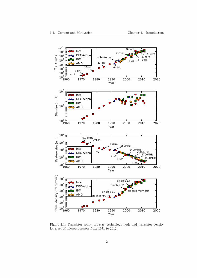
1.1 Transistor count, die size, technology node and transistor densityfor a set of microprocessors from 1971 to 2012. . . . . . . . . . . 2
1.2 Single Thread Performance . . . . . . . . . . . . . . . . . . . . . 5
1.3 Simulation speed gap. . . . . . . . . . . . . . . . . . . . . . . . . 6
1.4 Thesis timeline . . . . . . . . . . . . . . . . . . . . . . . . . . . . 9
1.5 Thesis organization. . . . . . . . . . . . . . . . . . . . . . . . . . 10
2.1 The Cell/B.E. microprocessor architecture [100]. . . . . . . . . . 14
2.2 The CellSim simulator. . . . . . . . . . . . . . . . . . . . . . . . . 16
2.3 Producer-consumer module example using CycleSim. . . . . . . . 19
2.4 Example of communication between Producer and Consumer mod-ules in CycleSim. . . . . . . . . . . . . . . . . . . . . . . . . . . . 19
2.5 Examples of architectures modeled using TaskSim. . . . . . . . . 21
2.6 Flow chart of execution-driven and trace-driven simulation. . . . 23
2.7 Breakdown of papers per simulation type in main computer ar-chitecture conferences from 2008 to 2012 . . . . . . . . . . . . . . 37
2.8 Breakdown of papers per maximum simulated number of cores inmain architecture conferences from 2008 to 2012 . . . . . . . . . 38
2.9 Breakdown of papers per simulation tool in main computer ar-chitecture conferences from 2008 to 2012 . . . . . . . . . . . . . . 39
2.10 Task-based implementation of the Fibonacci number recursive al-gorithm in (a) OpenMP 3.1, (b) Cilk and (c) Threading BuildingBlocks. . . . . . . . . . . . . . . . . . . . . . . . . . . . . . . . . . 41
2.11 Cholesky decomposition of a blocked matrix using OmpSs. . . . . 42
3.1 Execution of an application with a mutual exclusion using twothreads. . . . . . . . . . . . . . . . . . . . . . . . . . . . . . . . . 46
3.2 Simulation infrastructure scheme. . . . . . . . . . . . . . . . . . . 49
3.3 OmpSs application example and its corresponding traces for theTaskSim – NANOS++ simulation platform. . . . . . . . . . . . . 51
3.4 Implementation scheme. . . . . . . . . . . . . . . . . . . . . . . . 52
3.5 Scheme of a multithreaded application simulation that generates4 tasks and waits for their completion on two and four threads. . 54
3.6 Speed-up for different numbers of cores from 8 to 64 with respectto the execution with 8 cores. . . . . . . . . . . . . . . . . . . . . 55
3.7 Snapshot of the core activity visualization of a blocked-matrixmultiplication a with 1 task-generation thread, and b with a hi-erarchical task-generation scheme . . . . . . . . . . . . . . . . . . 56
ix
3.8 Application performance comparison for area-equivalent multi-core configurations. Speed-up with respect to the 16-core baseline. 57
4.1 Different application abstraction levels: (a) computation plusMPI calls, (b) computation plus parops, (c) memory accesses,and (d) instructions. . . . . . . . . . . . . . . . . . . . . . . . . . 63
4.2 Simulation error of the burst mode compared to the real execu-tion on an eight-core AMD Opteron 6128 processor for multiplenumbers of threads. . . . . . . . . . . . . . . . . . . . . . . . . . 74
4.3 Comparison of real and simulated execution time for a 4096×4096blocked-matrix Cholesky factorization using multiple block sizes. 76
4.4 Inout mode experiments on scratchpad-based architectures us-ing an FFT 3D application: (a) execution on a real Cell/B.E.,(b) simulation of a Cell/B.E. configuration, (c) simulation of aCell/B.E. configuration using a 128 B memory interleaving gran-ularity, (d) simulation of a 256-core SARC architecture configu-ration using a 4 KB interleaving granularity, and (e) simulationof a 256-core SARC architecture configuration using a 128 B in-terleaving granularity. Light gray show computation periods andblack shows periods waiting for data transfer completion. . . . . 78
4.5 Difference in number of misses between the mem and instr modesfor different simulated configurations using 4 and 32 cores, anddifferent interleaving granularities. . . . . . . . . . . . . . . . . . 79
5.1 Trace filtering: (a) example of a memory access trace, (b) howtrace filtering proceeds, and (c) the resulting filtered trace. . . . 82
5.2 Different multithread execution interleavings. On the left, theinvalidation occurs after LOAD D executes, so D hits. On the right,the invalidation occurs before D so D misses in this case. If thetrace is generated with the left execution, D will be filtered out,and if the scenario in the right is produced during simulation, Dwill not be there to miss. . . . . . . . . . . . . . . . . . . . . . . 83
5.3 Different dynamic scheduling decisions. Iterations of a parallelloop are scheduled in different ways. On the left, iterations 1and 2 are assigned to Thread 0, and 3 and 4 to Thread 1. Thatmakes iterations 2 and 4 to hit on their first memory access. Onthe right, 1 and 3 are assigned to Thread 0, and 2 and 4 to Thread1, making all of them to miss on their first memory access. If thetrace is generated using the left case and simulation leads to thecase on the right, the first accesses in iterations 2 and 4 wouldnot be present in the trace, and both misses could not be simulated. 83
5.4 Pathological case. The figure shows: (a) the pseudo-code of theapplication; (b) the task dependence graph showing tasks in cir-cles and the arrows between them are read-after-write (solid) andwrite-after-read (dashed) dependencies; (c) the execution in a sin-gle thread used for trace generation with the order in which tasksare executed; and (d) the simulation of the application on fourthreads showing to which threads tasks are dynamically sched-uled and their execution order. . . . . . . . . . . . . . . . . . . . 86

5.5 Pathological case execution time normalized to full trace with L2cache latency of 20 cycles. A small L2 cache latency can be hid-den by the superscalar core microarchitecture. Longer latenciesdelay L1 misses that are correctly simulated with our methodol-ogy (reset) and using the full trace. The naive method does notsimulate those L1 misses, as they were filtered out during tracegeneration. . . . . . . . . . . . . . . . . . . . . . . . . . . . . . . 87
5.6 OpenMP for loop construct. The figure shows: (a) a scheme ofthe execution flow of an OpenMP for ; (b) the original OpenMPC code and the intermediate C code generated by GCC, includingthe calls to the libgomp OpenMP runtime library. . . . . . . . . . 89
5.7 Trace generation and simulation process. . . . . . . . . . . . . . 905.8 Trace size reduction. . . . . . . . . . . . . . . . . . . . . . . . . . 935.9 Trace generation speed-up. . . . . . . . . . . . . . . . . . . . . . 935.10 Simulation accuracy. . . . . . . . . . . . . . . . . . . . . . . . . . 955.11 Simulation accuracy average across benchmarks and frequencies. 965.12 Simulation speed-up. . . . . . . . . . . . . . . . . . . . . . . . . . 975.13 Simulation speed-up average across benchmarks and frequencies. 98
6.1 Simulation example of a task-based application running on twothreads. (a) The simulation alternates between the simulatedthreads and the runtime system operation, to simulate the ac-tions specified in the events included in the trace. The runtimesystem performs the creation of tasks, and assign tasks to idlethreads (dashed line), such as Task 1 to Thread 1. (b) The simu-lation engine does not account the timing of the runtime systemoperations, and only simulates the timing of the sequential sec-tions in the trace. . . . . . . . . . . . . . . . . . . . . . . . . . . . 102
6.2 Simplified pseudo-code of the main NANOS++ operations, andthe actions on shared resources: task dependence graph and readyqueue. Checks and updates of shared data are protected by locksor atomic operations depending on their granularity. . . . . . . . 104
6.3 Runtime system operation variability. (a) Task creation cost dis-tribution of Cholesky factorization run on eight threads for twodifferent throttling limits. (b) Breakdown of the lock contentiontime of Cholesky decomposition run on four, eight and sixteenthreads for four different throttling limits. . . . . . . . . . . . . . 105
6.4 Simulation example with host time only (left) and host time plussimulation of locks (right). . . . . . . . . . . . . . . . . . . . . . . 106
6.5 Normalized execution time real (a) and simulated (b,c,d) for ablocked-matrix multiplication using 64×64 blocks. . . . . . . . . 108
6.6 Task creation execution time of the H.264 decoder skeleton bothin the real machine and using the host simulation approach usingmultiple numbers of threads. . . . . . . . . . . . . . . . . . . . . 109


List of Tables
2.1 Main advantages and disadvantages of trace-driven simulationover execution-driven simulation . . . . . . . . . . . . . . . . . . 28
2.2 Task-based programming models . . . . . . . . . . . . . . . . . . 40
4.1 Summary of TaskSim simulation modes. This includes their ap-plicability on computer architecture evaluations, and their fea-tures also comparing to state-of-the-art (SOA) simulators . . . . 69
4.2 Comparison of abstraction levels in existing simulators in termsof simulation speed and modeling detail . . . . . . . . . . . . . . 71
4.3 TaskSim main configuration parameters. The experiments in Sec-tion 4.5 use the default values unless it is explicitly stated otherwise 73
4.4 List of benchmarks, including their label used in the charts anda description of their configuration parameters. . . . . . . . . . . 74
4.5 Cholesky factorization of a 4096×4096 blocked-matrix using dif-ferent block sizes. The table shows the number of tasks, the av-erage task execution time and the comparison of real executionand simulation for four and eight threads. . . . . . . . . . . . . . 75
5.1 TaskSim simulation parameters. . . . . . . . . . . . . . . . . . . . 915.2 OmpSs benchmarks. . . . . . . . . . . . . . . . . . . . . . . . . . 92
xiii

Chapter 1
Introduction
1.1 Context and Motivation
1.1.1 Chip Multiprocessors
A microprocessor is an integrated circuit (chip) that incorporates the centralprocessing unit (CPU) of a von Neumann-style computing system. The firstmicroprocessors appeared in the early 1970s [176, 74]. Since then, the numberof transistors on a chip has increased exponentially. This fact was observed byGordon Moore in 1965, a claim that is popularly known as Moore’s law [124].The rate at which the number of transistors on a chip increased was set todouble every year in 1965. In 1975, Moore adjusted his observation to doubleevery two years [123]. This observation has served as an industry driver. Com-panies’ roadmaps target Moore’s law transistor count growth rate, which setstargets for research and development divisions and results in the developmentand introduction of new technology nodes to achieve the required transistordensity.
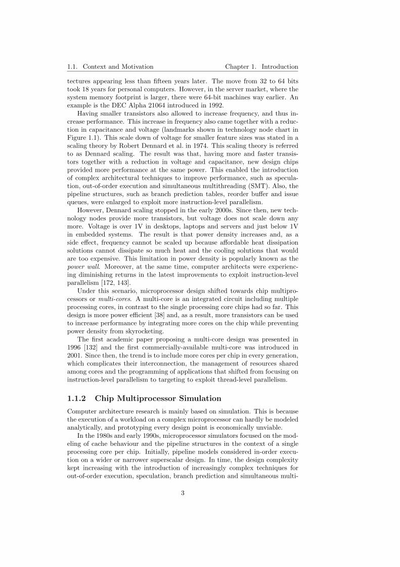
Figure 1.1 shows the transistor count per chip, die size, technology nodeand transistor density for a set of microprocessor from 1971 to 2012. Dataactually confirms Moore’s law, and shows a 2x increase in transistor count perchip every two years. This increase was a combination of higher transistordensity (+22%/year) and larger die size (+15%/year) until 1992. Since 1992,die size has not increased significantly. Server microprocessors have larger diesizes between 300 and 600 mm2, while desktop microprocessor die sizes arebetween 100 and 300 mm2. However, transistor density has increased 2x everytwo years (+40%/year) since 1992, thus keeping up with Moore’s law transistorcount growth rate. This increase in transistor density growth rate was partiallythanks to the inclusion of on-chip caches. Caches are more regular than otherpipeline logic structures and thus have a higher transistor density.
The availability of more transistors allowed architects to integrate devices,that were so far out of the chip, on the chip (landmarks shown in transistordensity chart in Figure 1.1). Examples are the inclusion of floating-point units,caches and memory controllers. Also, it allowed architects to build more com-plex architectures. First, the bit width of data and address paths was increasedto improve performance and to be able to reference a larger address space. Thefirst microprocessors had 4- and 8-bit data paths, with 16- and 32-bit archi-
1
1.1. Context and Motivation Chapter 1. Introduction
1960 1970 1980 1990 2000 2010 2020Year
1031041051061071081091010
Tran
sistors
4-bit8-bit
16-bit32-bit
64-bit
out-of-orderSMT
2-core4-core
6-core8-core
1+8-core
IntelDEC-AlphaIBMAMD
1960 1970 1980 1990 2000 2010 2020Year
101
102
103
Die size (m
m²) Intel
DEC-AlphaIBMAMD
1960 1970 1980 1990 2000 2010 2020Year
101
102
103
104
105
Feature size (n
m) 0.74MHz
2MHz12MHz 150MHz
1400MHz2800MHz
4700MHz3500MHz
5V3.1V
1.6V1.25V
IntelDEC-AlphaIBMAMD
1960 1970 1980 1990 2000 2010 2020Year
102103104105106107
Tran
s. den
sity (trans/m
m²)
on-chip FPUon-chip L1
on-chip L2on-chip L3
on-chip mem ctlr
IntelDEC-AlphaIBMAMD
Figure 1.1: Transistor count, die size, technology node and transistor densityfor a set of microprocessors from 1971 to 2012.
2
1.1. Context and Motivation Chapter 1. Introduction
tectures appearing less than fifteen years later. The move from 32 to 64 bitstook 18 years for personal computers. However, in the server market, where thesystem memory footprint is larger, there were 64-bit machines way earlier. Anexample is the DEC Alpha 21064 introduced in 1992.
Having smaller transistors also allowed to increase frequency, and thus in-crease performance. This increase in frequency also came together with a reduc-tion in capacitance and voltage (landmarks shown in technology node chart inFigure 1.1). This scale down of voltage for smaller feature sizes was stated in ascaling theory by Robert Dennard et al. in 1974. This scaling theory is referredto as Dennard scaling. The result was that, having more and faster transis-tors together with a reduction in voltage and capacitance, new design chipsprovided more performance at the same power. This enabled the introductionof complex architectural techniques to improve performance, such as specula-tion, out-of-order execution and simultaneous multithreading (SMT). Also, thepipeline structures, such as branch prediction tables, reorder buffer and issuequeues, were enlarged to exploit more instruction-level parallelism.
However, Dennard scaling stopped in the early 2000s. Since then, new tech-nology nodes provide more transistors, but voltage does not scale down anymore. Voltage is over 1V in desktops, laptops and servers and just below 1Vin embedded systems. The result is that power density increases and, as aside effect, frequency cannot be scaled up because affordable heat dissipationsolutions cannot dissipate so much heat and the cooling solutions that wouldare too expensive. This limitation in power density is popularly known as thepower wall. Moreover, at the same time, computer architects were experienc-ing diminishing returns in the latest improvements to exploit instruction-levelparallelism [172, 143].
Under this scenario, microprocessor design shifted towards chip multipro-cessors or multi-cores. A multi-core is an integrated circuit including multipleprocessing cores, in contrast to the single processing core chips had so far. Thisdesign is more power efficient [38] and, as a result, more transistors can be usedto increase performance by integrating more cores on the chip while preventingpower density from skyrocketing.
The first academic paper proposing a multi-core design was presented in1996 [132] and the first commercially-available multi-core was introduced in2001. Since then, the trend is to include more cores per chip in every generation,which complicates their interconnection, the management of resources sharedamong cores and the programming of applications that shifted from focusing oninstruction-level parallelism to targeting to exploit thread-level parallelism.
1.1.2 Chip Multiprocessor Simulation
Computer architecture research is mainly based on simulation. This is becausethe execution of a workload on a complex microprocessor can hardly be modeledanalytically, and prototyping every design point is economically unviable.
In the 1980s and early 1990s, microprocessor simulators focused on the mod-eling of cache behaviour and the pipeline structures in the context of a singleprocessing core per chip. Initially, pipeline models considered in-order execu-tion on a wider or narrower superscalar design. In time, the design complexitykept increasing with the introduction of increasingly complex techniques forout-of-order execution, speculation, branch prediction and simultaneous multi-
3

1.1. Context and Motivation Chapter 1. Introduction
threading. On the other hand, the design space of the cache hierarchy includedcache size, associativity, latency and writing policies for one or two cache levels.
However, with the introduction of multi-cores, microprocessor simulationturned into the simulation of a parallel machine. The simulation of a parallelarchitecture is even more challenging than simulating a single core. Severalexecution streams stress not only core-private components but also shared re-sources in the architecture. These shared components include shared caches,off-chip memory and the on-chip interconnection among cores. Modeling suchsharing and resource contention is already challenging for multiprogrammedworkloads. However, for multithreaded applications, it is also sensitive to thelevel of parallelism, inter-thread data sharing and thread synchronization of theparticular application. To faithfully account for these effects, the simulationmodel requires the inclusion, among others, of cache coherence protocols, cachedata placement policies, network arbitration and cache partitioning techniques.
Many of the modeling challenges of multi-core simulation are not new, asthey were already present when simulating shared-memory multiprocessor sys-tems with cache coherency across multiple chips. However, there are fundamen-tal differences of having such a parallel system on a single chip compared tomulti-chip multiprocessors. Communication latencies are lower thanks to faston-chip interconnection networks. And memory bandwidth is also lower becausean increasing amount of processing cores have to share a limited amount of pinsto access off-chip memory.
Due to these fundamental differences, researchers need to assess the applica-bility of techniques developed for shared-memory multiprocessors in the contextof multi-cores. But, at the same time, multi-core designs also open new researchopportunities that are unique for multi-cores. As a result, multi-core simulationbecomes a fundamental tool for either revisiting existing ideas and explore newones.
1.1.3 The Simulation Speed Gap
Computer architecture simulation is mainly a single-threaded problem becausethe fine-grain interaction of the components in the chip limits its parallelization.Most computer architecture simulators are thus sequential and, as a result, sim-ulation speed highly depends on the single-thread performance of the machinewere the simulator is running.
While the complexity of microprocessors keeps increasing, single-thread per-formance is not increasing at the same pace. The efforts to develop or im-prove techniques to exploit instruction level parallelism have decreased due todiminishing returns and power density issues. This shifted the focus of com-puter architects to higher aggregated multi-core performance rather than highersingle-thread performance.
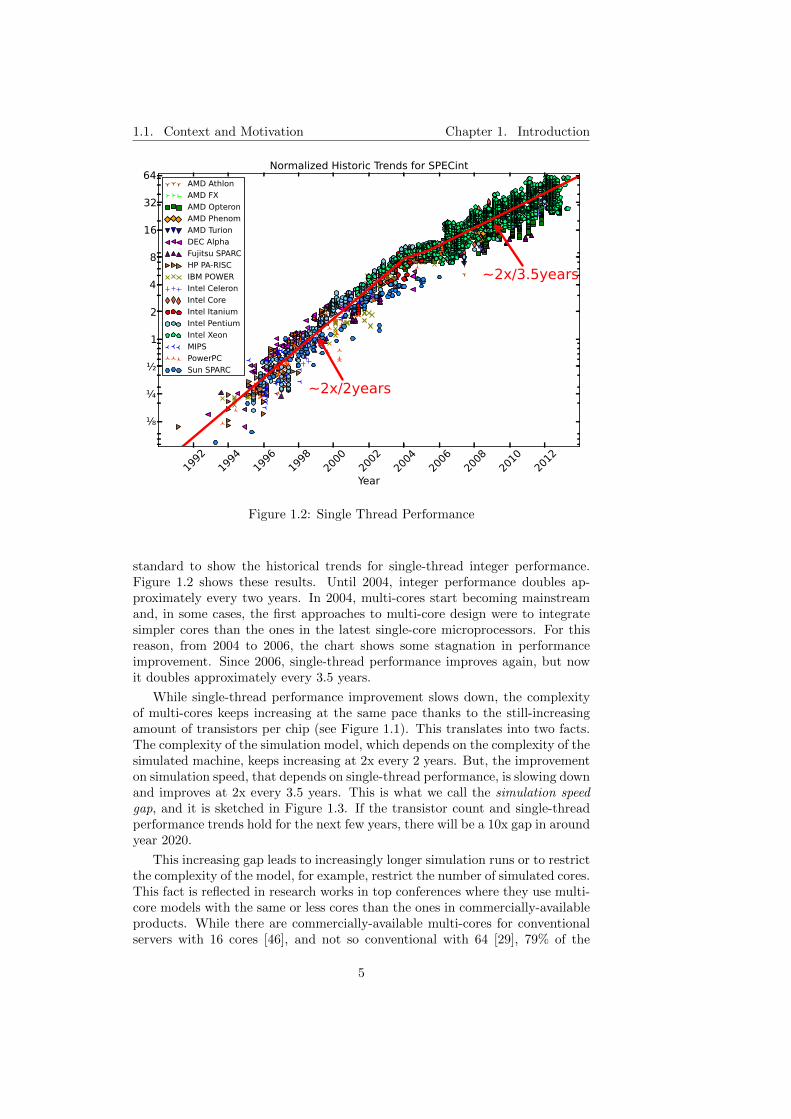
A popular benchmark suite to measure single-thread performance is SPEC(Standard Performance Evaluation Corporation) CPU. The SPEC CPU bench-mark suite is divided in two subsets: integer (CINT) and floating-point (CFP)benchmarks. We focus on the SPEC CINT benchmarks because computer sim-ulation code is mainly integer code. We have gathered the SPECint results fora set of microprocessors from 1991 to 2013 and adjusted them1 to the 2006
1We use the methodology in J. Preshing’s blog [137], abiding the SPEC fair use rules [10].
4
1.1. Context and Motivation Chapter 1. Introduction
1992
1994
1996
1998
2000
2002
2004
2006
2008
2010
2012
Year
⅛
¼
½
1
2
4
8
16
32
64
~2x/2years
~2x/3.5years
Normalized Historic Trends for SPECintAMD AthlonAMD FXAMD OpteronAMD PhenomAMD TurionDEC AlphaFujitsu SPARCHP PA-RISCIBM POWERIntel CeleronIntel CoreIntel ItaniumIntel PentiumIntel XeonMIPSPowerPCSun SPARC
Figure 1.2: Single Thread Performance
standard to show the historical trends for single-thread integer performance.Figure 1.2 shows these results. Until 2004, integer performance doubles ap-proximately every two years. In 2004, multi-cores start becoming mainstreamand, in some cases, the first approaches to multi-core design were to integratesimpler cores than the ones in the latest single-core microprocessors. For thisreason, from 2004 to 2006, the chart shows some stagnation in performanceimprovement. Since 2006, single-thread performance improves again, but nowit doubles approximately every 3.5 years.
While single-thread performance improvement slows down, the complexityof multi-cores keeps increasing at the same pace thanks to the still-increasingamount of transistors per chip (see Figure 1.1). This translates into two facts.The complexity of the simulation model, which depends on the complexity of thesimulated machine, keeps increasing at 2x every 2 years. But, the improvementon simulation speed, that depends on single-thread performance, is slowing downand improves at 2x every 3.5 years. This is what we call the simulation speedgap, and it is sketched in Figure 1.3. If the transistor count and single-threadperformance trends hold for the next few years, there will be a 10x gap in aroundyear 2020.
This increasing gap leads to increasingly longer simulation runs or to restrictthe complexity of the model, for example, restrict the number of simulated cores.This fact is reflected in research works in top conferences where they use multi-core models with the same or less cores than the ones in commercially-availableproducts. While there are commercially-available multi-cores for conventionalservers with 16 cores [46], and not so conventional with 64 [29], 79% of the
5

1.2. Thesis contributions Chapter 1. Introduction
2002 2004 2006 2008 2010 2012 2014 2016 2018 2020 2022Year
hola
~2x/2years
~2x/3.5years
10x
Transistor countSingle-thread performanceSimulation speed gap
Figure 1.3: Simulation speed gap.
research papers in major computer architecture conferences between 2009 and2012 simulate at most 16 cores, and only 5% simulate more than 64 cores 2.
1.2 Thesis contributions
The simulation speed gap poses a challenge on computer architects to simulatelarge multi-core designs. To complete the simulation of large multi-cores in areasonable time, we require higher simulation speeds. Researchers are conciousof this problem, and they have proposed several techniques to reduce simulationtime such as statistical simulation, sampling and parallel simulation.
The approach in this thesis is to raise the level of abstraction of the simula-tion model. This allows to increase simulation speed at the expense of modelingaccuracy in order to reduce simulation time. Some reputed researchers advocatefor this approach [39, 180] and previous works have applied it in other scenariossuch as cluster and network simulation [24, 120].
To implement high levels of abstraction, we advocate for the use of trace-driven simulation. However, one of the most important limitations of trace-driven simulation is precisely its inability to reproduce the dynamic behaviorof multithreaded applications, which are absolutely necessary for the evaluationof multi-core systems. This limitation is because the application behavior inmultiple threads is statically captured in a trace and does not change for differentsimulated configurations as it would happen in a real machine.
To overcome this limitation, the first contribution in this thesis is:
2Check Section 2.6 for more simulation statistics in computer architecture conferences.
6

1.2. Thesis contributions Chapter 1. Introduction
• A simulation methodology for simulating multithreaded applicationsrunning on multi-cores using trace-driven simulation. In this simula-tion methodology, we combine the trace-driven simulation of the timing-independent parts of the application, with the execution of timing-dependentoperations at simulation time. This way, run-time decisions are madebased on the simulated machine and are thus different for different config-urations as it would happen in the real machine. This work is supportedby the following papers:
[150] A. Rico, A. Duran, F. Cabarcas, Y. Etsion, A. Ramirez, M. Valero.Trace-driven Simulation of Multithreaded Applications. In Proceed-ings of the IEEE International Symposium on Performance Analysisof Systems and Software, ISPASS ’11, pages 87–96, Apr. 2011.
[151] A. Rico, A. Duran, A. Ramirez, M. Valero. Simulating Dynamically-Scheduled Multithreaded Applications Using Traces. IEEE Micro.Submitted for publication.
Once we can reliably use trace-driven simulation for multithreaded applica-tions running on multi-cores, we use it to raise the level of abstraction of simu-lation. However, several questions arise when using higher levels of abstractionregarding what are the right levels of abstraction, their insight, accuracy andsimulation speed.
The second contribution in this thesis is:
• Two fast high-level simulation modes along with two lower-level ones.These simulation modes at different levels of abstraction are based on ourdefinition of application abstraction levels and target application scala-bility, accelerator architectures, memory system and pipeline modeling,respectively. We evaluate the insight of these simulation modes, their ac-curacy and their simulation speed compared to the levels of abstractionused in popular computer architecture simulators. This contribution issupported by the following publication:
[148] A. Rico, F. Cabarcas, C. Villavieja, M. Pavlovic, A. Vega, Y. Etsion,A. Ramirez, M. Valero. On the Simulation of Large-Scale Architec-tures Using Multiple Application Abstraction Levels. ACM Trans.Archit. Code Optim., 8(4):36:1–36:20, 2012.
One of the abstraction levels in our definition targets multi-core memorysimulation. This level of abstraction uses an abstract model for processingcores that focus mainly on memory accesses. To speed up memory simulation,previous works use filtered traces that include only L1 cache misses to avoid thecost of simulating L1 hits assuming that these do not imply additional delaysin the simulated application. This technique, called trace stripping [138], hasbeen successfully used in the past for single-thread scenarios. However, littlework has been done to use it for multithreaded applications, in which inherentinaccuracies appear due to cache invalidations. A filtered hit may miss in amultithreaded scenario due to the invalidation of the accessed data from a writein another cache.
The third contribution in this thesis is:
7

1.3. Timeline Chapter 1. Introduction
• A trace generation technique based on the structure of multithreadedapplications that captures in the trace L1 hits that may potentially missin a multithreaded application execution due to invalidations. With thistechnique, we cover potential invalidations due to different thread inter-leavings and different dynamic schedulings. Our evaluation shows thatour technique consistently reduces the error of the state-of-the-art tech-nique at the expense of small losses in trace size reduction and simulationspeed-up. This work is supported by the following publication:
[154] A. Rico, A. Ramirez, M. Valero. Trace Filtering of MultithreadedApplications for CMP Memory Simulation. In Proceedings of theIEEE International Symposium on Performance Analysis of Systemsand Software, ISPASS ’13, pages 134–135, Apr. 2013.
One of the potential inaccuracies of our simulation methodology in our firstcontribution is that the execution of timing-dependent operations is not exposedto the simulator, and thus cannot be accurately accounted in the applicationtiming modeling.
The fourth contribution in this thesis is:
• A fast high-level timing model for timing-dependent operationsthat are executed at simulation time using our simulation methodology.This timing model is based on the execution of these operations on thehost machine to account for different algorithm complexities and run-time application states. Additionally, we also model their contention onaccessing data structures shared by multiple threads on the simulatedapplication.
1.3 Timeline
Figure 1.4 shows a timeline of relevant events related to the work in this thesisto put it in context. At the top of the figure, we show the releases of multi-core commercial products. The trend followed by the main manufacturers is toincrease the number of cores per chip in every new generation of multi-cores. Asexplained in previous sections, this motivates our work to bridge the simulation-speed gap.
The work in this thesis has contributed to several projects. From January2006 to December 2009, we contributed to the SARC project with the devel-opment of CellSim (see Section 2.1). CellSim served to carry out the workof several partners in the project, leading to multiple publications and PhDdissertations (see Section 7.2). CellSim was also the base for SARCSim: an ex-tension of CellSim including timing models from other SARC partners, such asmodels of extended vector accelerators and scalable inter-core communicationmechanisms.
In the context of the MareIncognito project (from January 2007 to December2009), CellSim was relevant in the research for the design of next-generationCell/B.E. microprocessors (see Section 2.1.1). From March 2010 to February2013 we contributed to the ENCORE project. The simulation methodologiesproposed in this thesis were used in ENCORE for the evaluation of explicitmanagement of coherent and non-coherent cache hierarchies. Also, the analysis
8

1.3. Timeline Chapter 1. Introduction
2006 2007 2008 2009 2010 2011 2012 2013
Multicores
Projects
Milestones
Other
Simulators
CellSim
Tut
orial
Internships
IBM9 cores
SARC ENCORE
MareIncognito
IBM ARM
TaskS
im
Tut
orial
TaskS
im
MT A
pps.
TaskS
im
Abs
tr. lev
els
TaskS
im
Trace filt
gem5Graphite SniperRigel
Intel2 cores
AMD2 cores
AMD4 cores
Intel4 cores
AMD6 cores
Intel6,8 cores
IBM8 cores
Intel10 cores
AMD8 cores
Sun8 cores
Sun16 cores
GEMS M5 PTLsim
Figure 1.4: Thesis timeline
of the runtime system we carried out for the simulation of the runtime systemtiming (see Chapter 6) was used in ENCORE to understand the overheads ofthe several components in the runtime system.
The course of this thesis was interrupted by two industrial internships. Thefirst one at the IBM TJ Watson Research Center (Yorktown Heights, NY, USA)for the development of a vector accelerator took place from October 2008 toDecember 2009. The second internship was at ARM Ltd. (Cambridge, UK)from August 2012 to November 2012 and focused on the evaluation of the ARMCortex-A family of microprocessors for high performance computing.
Some milestones worth mentioning as outcomes of the work in this thesisare the following:
• CellSim Tutorial. We performed a full-day tutorial on our CellSimsimulator (see Section 2.1) in the Parallel Architectures and CompilationTechniques (PACT) conference at Brasov, Romania, on September 2007.
• TaskSim Tutorial. We performed a tutorial for the ENCORE projectpartners on our TaskSim simulator (see Section 2.2) on March 2010.
• Publication of ”Trace-Driven Simulation of Multithreaded Ap-plications”. Publication in Proceedings of the International Sympo-sium on Performance Analysis of Systems and Software (ISPASS) 2011at Austin, TX, USA, on April 2011.
• Publication of ”On the Simulation of Large-Scale ArchitecturesUsing Multiple Application Abstraction Levels”. Publication inthe ACM Transactions on Architecture and Compiler Optimization (TACO),Vol. 8, No. 4, Article 36, January 2012.
9

1.4. Thesis Organization Chapter 1. Introduction
• Publication of ”Trace Filtering of Multithreaded Applicationsfor CMP Memory Simulation”. Publication in International Sympo-sium on Performance Analysis of Systems and Software (ISPASS) 2013 atAustin, TX, USA, on April 2013.
In the course of this thesis, other groups in the computer architecture com-munity working on simulation of multi-cores published their tools in relatedconferences and journals. Some of them shown at the bottom of Figure 1.4 areGEMS, M5, PTLsim, Rigel, Graphite, gem5 and Sniper. We cover these worksin Section 2.5.
1.4 Thesis Organization
Figure 1.5 illustrates the organization of this document in the several chaptersit is composed of.
1. Introduction
7. Conclusions
Publications Impact Future Work
3. Simulating Multithreaded
Applications Using Traces
4. Multiple Levels
of Abstraction
5. Trace Filtering of
Multithreaded
Applications
6. Modeling the
Runtime System
Timing
2. Background
CellSim TaskSim
Figure 1.5: Thesis organization.
After this introductory chapter, we devote Chapter 2 to cover related workfor this thesis. In this chapter, we include an explanation of CellSim andTaskSim, two simulators to which we contributed to develop in the course of
10

1.4. Thesis Organization Chapter 1. Introduction
this thesis. The lessons learned in the development of CellSim motivated thedevelopment of TaskSim and the research that led to the contributions in thisthesis. The rest of the background in Chapter 2 is general and relevant for therest of the document.
We cover our contributions in Chapters 3, 4, 5 and 6. We include generalrelated work and state of the art in Chapter 2 and the specific related work andstate of the art relevant to each contribution in each one of the correspondingchapters.
Chapter 3 explains and evaluates the first contribution of this thesis: asimulation methodology for simulating multithreaded applications using a trace-driven simulation approach. This simulation methodology enables the works inChapters 4 and 5 and motives the work in Chapter 6.
Chapter 4 covers our definition of multiple application abstraction levels,the corresponding simulation modes at multiple levels of abstraction, and theirevaluation in terms of insight, accuracy and simulation speed. In Chapter 5 wecover the description and evaluation of our trace filtering technique for multi-threaded applications and in Chapter 6 we cover our high-level timing modelfor timing-dependent operations to be used with the simulation methodology inChapter 3.
Finally, we conclude this thesis in Chapter 7 with our contributions andassociated publications, the impact of our work in other works and some rec-ommendations for future work.
11

1.4. Thesis Organization Chapter 1. Introduction
12

Chapter 2
Background
In this chapter we cover related and relevant work for this thesis. First weintroduce CellSim, a simulator we developed for modeling the Cell/B.E. micro-processor. The difficulties and experiences during the development of CellSimmotivated us to initiate research with the objective of exploring new simulationtechniques to reduce simulation time by raising the level of abstraction.
We also cover related work on other techniques for reducing simulation time.This includes techniques used in state-of-the-art simulators such as statisticalsimulation, sampling and parallel simulation. We also cover works using field-programmable gate arrays (FPGA) prototyping with the aim of speeding upcomputer simulation.
We explain a set of existing multi-core simulators that are relevant for thework in this thesis either because the are widely used or because they implementsome of the simulation time reduction techniques explained before. We alsoinclude a survey on the use of these simulation tools and techniques in majorcomputer architecture conferences.
Finally, we give an overview of task-based parallel programming models.This background is important because the multithreaded applications drivingthe work in this thesis are programmed in OmpSs [68], a task-based program-ming model.
2.1 CellSim
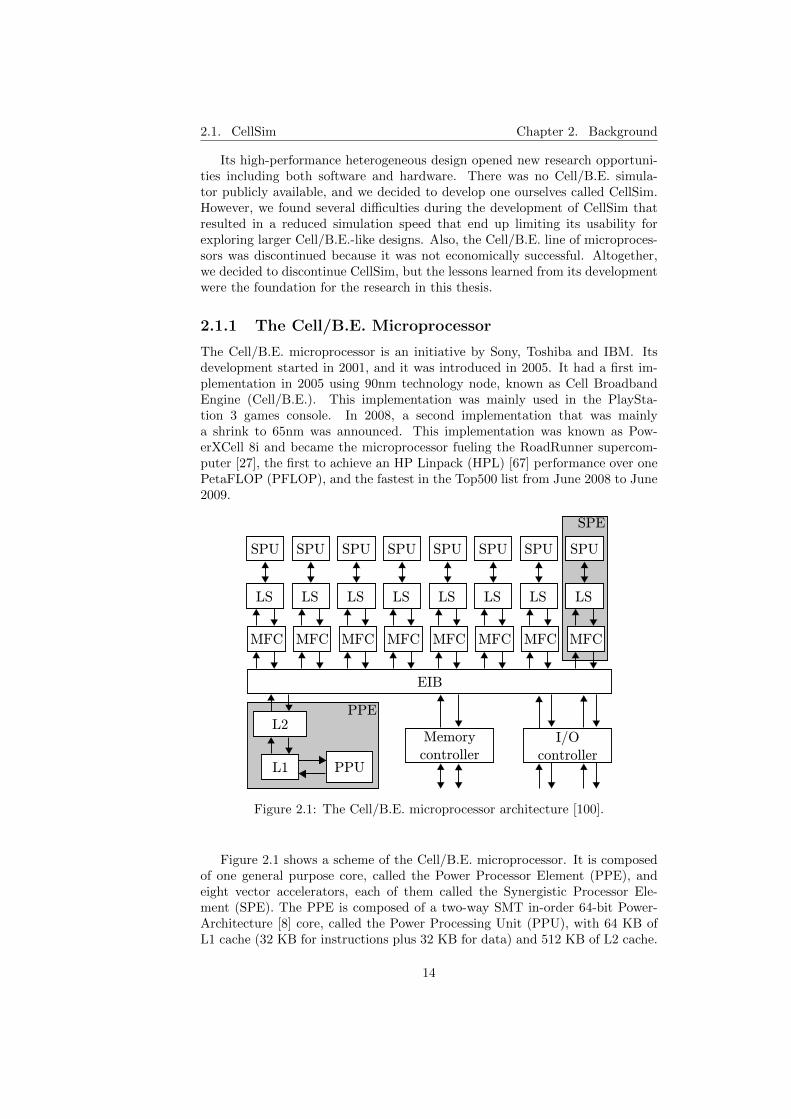
CellSim [49, 147, 50, 51, 142] is a simulator modeling the Cell Broadband En-gine (Cell/B.E.) microprocessor [100]. The introduction of the Cell/B.E. was abreakthrough due to its unique characteristics. It was the first high-performanceheterogeneous multi-core. Heterogeneous designs have been widely used in theembedded market. Microprocessors such as the NXP Viper [71], TI OMAP [56]include a general-purpose core, a very-long-instruction-word (VLIW) core anda set of multimedia accelerators such as video and audio encoders and decoders.However, the Cell/B.E. was the first to have an impact on high-performancecomputing (HPC) although it was initially designed for the video-game mar-ket, precisely as the microprocessor of the Sony PlayStation 3 games console. Aproof of its impact in HPC is that the number one supercomputer in the Top500list [11] of June 2008 was mainly composed of Cell/B.E. microprocessors.
13
2.1. CellSim Chapter 2. Background
Its high-performance heterogeneous design opened new research opportuni-ties including both software and hardware. There was no Cell/B.E. simula-tor publicly available, and we decided to develop one ourselves called CellSim.However, we found several difficulties during the development of CellSim thatresulted in a reduced simulation speed that end up limiting its usability forexploring larger Cell/B.E.-like designs. Also, the Cell/B.E. line of microproces-sors was discontinued because it was not economically successful. Altogether,we decided to discontinue CellSim, but the lessons learned from its developmentwere the foundation for the research in this thesis.
2.1.1 The Cell/B.E. Microprocessor
The Cell/B.E. microprocessor is an initiative by Sony, Toshiba and IBM. Itsdevelopment started in 2001, and it was introduced in 2005. It had a first im-plementation in 2005 using 90nm technology node, known as Cell BroadbandEngine (Cell/B.E.). This implementation was mainly used in the PlaySta-tion 3 games console. In 2008, a second implementation that was mainlya shrink to 65nm was announced. This implementation was known as Pow-erXCell 8i and became the microprocessor fueling the RoadRunner supercom-puter [27], the first to achieve an HP Linpack (HPL) [67] performance over onePetaFLOP (PFLOP), and the fastest in the Top500 list from June 2008 to June2009.
L2
SPU
LS
MFC
EIB
SPU
LS
MFC
SPU
LS
MFC
SPU
LS
MFC
SPU
LS
MFC
SPU
LS
MFC
SPU
LS
MFC
SPU
LS
MFC
SPE
L1 PPU
PPE
Memory
controller
I/O
controller
Figure 2.1: The Cell/B.E. microprocessor architecture [100].
Figure 2.1 shows a scheme of the Cell/B.E. microprocessor. It is composedof one general purpose core, called the Power Processor Element (PPE), andeight vector accelerators, each of them called the Synergistic Processor Ele-ment (SPE). The PPE is composed of a two-way SMT in-order 64-bit Power-Architecture [8] core, called the Power Processing Unit (PPU), with 64 KB ofL1 cache (32 KB for instructions plus 32 KB for data) and 512 KB of L2 cache.
14
2.1. CellSim Chapter 2. Background
Both levels of cache are private to the PPE. The PPE executes the operatingsystem and acts as a controller of the eight SPEs.
An SPE includes a SIMD processing core, called the Synergistic ProcessingUnit (SPU), a 256 KB local memory called Local Store (LS), and a direct-memory-access (DMA) engine called the Memory Flow Controller (MFC). TheSPU is a two-wide-issue in-order core with a new SIMD-based instruction setarchitecture (ISA) [12]. It incorporates just SIMD execution units and has sim-ple hint-based branch prediction because it targets energy efficiency for regulardata-intensive codes. The SPU can only access data in the LS. The LS worksas an scratchpad memory. To move data in and out of the scratchpad memory,it must be done using DMA commands in the MFC.
The eight SPEs and the PPE are connected using a three-ring intercon-nection network called the Element Interconnect Bus (EIB). The EIB also gaveaccess to off-chip memory through the on-chip memory controller and to off-chipdevices through the input/output (I/O) controller.
Both implementations of the Cell/B.E. were clocked at 3.2 GHz and provideda peak single-precision floating-point performance of 204.8 GFLOPS using alleight SPEs. The PowerXCell 8i included, unlike its predecessor, fully-pipelineddouble-precision floating-point units in the SPEs that provided 102.4 GFLOPSup from 12.8 GFLOPS in the first implementation. These facts confirmed how,although the first implementation of the Cell/B.E. targeted multimedia com-puting, for which double-precision floating-point is irrelevant, the interest ofthe scientific community led to a second implementation providing full-fledgeddouble-precision floating-point capabilities.
However, the Cell/B.E. architecture also has some weaknesses. Program-ming to achieve high performance is tedious. The non-coherent nature of theLSs requires explicit data movement and the SIMD nature of the SPEs requiresprogramming with vector data structures and deal with alignment, gatheringand scattering of data while using close-to-assembler semantics. These pro-grammability limitations added to the high design and development costs thatled to its discontinuation.
2.1.2 CellSim Design
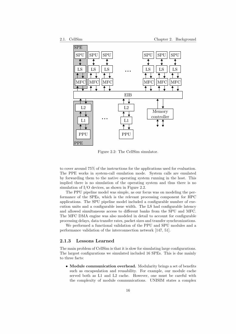
Our approach to simulating the Cell/B.E. was to use a modular infrastructure.Using a monolithic approach, apart from being generally bad software engineer-ing practice, would lead to many dependencies among architecture components.Having a modular infrastructure allows having encapsulated components witha clear interface among them. For this purpose, we employed the UNISIM in-frastructure [20] that allows to describe an architecture by specifying a set ofmodules and the connections among them.
In CellSim, the PPU, caches, SPU, LS, MFC, EIB and memory controllerare independent modules. Figure 2.2 shows a scheme of CellSim including itsmodules and interconnections. The design allows a configurable number of PPEsand SPEs. This allowed to set up a Cell/B.E. configuration with one PPE andeight SPEs, and also exploring future Cell/B.E. implementations with morePPEs and SPEs.
CellSim is an execution-driven simulator. This implies that it has to supporttwo different ISAs, the 64-bit Power ISA and the SPU ISA. Since the SPU ISAwas new, we had to implement it from scratch and almost completely as we need
15
2.1. CellSim Chapter 2. Background
SPU
LS
MFC
EIB
SPU
LS
MFC
Memory
controller
L2
L1
PPU
PPE
L2
L1
PPU
...
SPE
...
SPU
LS
MFC
SPU
LS
MFC
SPU
LS
MFC
SPU
LS
MFC
Figure 2.2: The CellSim simulator.
to cover around 75% of the instructions for the applications used for evaluation.The PPE works in system-call emulation mode. System calls are emulatedby forwarding them to the native operating system running in the host. Thisimplied there is no simulation of the operating system and thus there is nosimulation of I/O devices, as shown in Figure 2.2.
The PPU pipeline model was simple, as our focus was on modeling the per-formance of the SPEs, which is the relevant processing component for HPCapplications. The SPU pipeline model included a configurable number of exe-cution units and a configurable issue width. The LS had configurable latencyand allowed simultaneous access to different banks from the SPU and MFC.The MFC DMA engine was also modeled in detail to account for configurableprocessing delays, data transfer rates, packet sizes and transfer synchronizations.
We performed a functional validation of the PPU and SPU modules and aperformance validation of the interconnection network [147, 51].
2.1.3 Lessons Learned
The main problem of CellSim is that it is slow for simulating large configurations.The largest configurations we simulated included 16 SPEs. This is due mainlyto three facts:
• Module communication overhead. Modularity brings a set of benefitssuch as encapsulation and reusability. For example, our module cacheserved both as L1 and L2 cache. However, one must be careful withthe complexity of module communications. UNISIM states a complex
16

2.1. CellSim Chapter 2. Background
communication protocol between modules. The sender module writes thedata in the output port at the beginning of the cycle. Then, the receivingmodule accepts it or rejects it. If the receiver accepts it, then the sendercan enable it or not. This three-way protocol unnecessarily complicatescommunication and introduces a large overhead for every interconnectionport every cycle.
• Software emulation. Due to the execution-driven nature of CellSim,instructions must be functionally simulated (emulated). This has somebenefits as we explain in Section 2.3. From a developer’s point of view,implementing the instruction set functionality provides a deep understand-ing of the core features and capabilities. However, from a performance-prediction perspective, emulation adds a simulation overhead for everyinstruction, something that seems unnecessary if the objective is just todetermine the instruction timing.
An additional problem of execution-driven simulation appears when themodel is tied to the ISA. In the case of CellSim, the SPU ISA was spe-cific to the Cell/B.E. This restricted the flexibility of CellSim. Whenthe Cell/B.E. was discontinued, software development for the Cell/B.E.stopped and we found ourselves with a restricted amount of applicationsto feed our simulator with.
In modern execution-driven simulators, functional simulation is decoupledfrom the timing model. The functional simulation component translatesthe instructions to an intermediate ”ISA-independent” representation thatis fed to the timing model. This way multiple ISAs can be supported andthe timing model becomes ISA independent [36].
• Detailed modeling. The use of execution-driven simulation allows adetailed modeling of the processing cores because all the information aboutthe running instruction is available for the timing model. This is usefulfor detailed modeling of a specific core. However, when that detailedmodel is replicated for a large number of cores, simulation speed (cyclesper second) drops dramatically (typically super linearly). Some of ourexperiments focused on the interconnect and off-chip memory bandwidthwith an increasing number of SPEs. In these cases, most of the time wasspent in the detailed modeling of the SPU and LS, while our explorationwas not focused in those components. Also, for interconnect and memorybandwidth studies, it is interesting to find the sweet spot design thatbest manages contention with an increasing number of cores. However,simulating more than sixteen SPEs using such detailed models requiredlong simulation times. As an example, simulations of sixteen SPEs andone PPE using CellSim run at approximately 9 kilo cycles per second(140 kilo instructions per second (KIPS)) on a Pentium 4 at 3 GHz. Thisis a slowdown of 33 333x compared to native execution.
The lessons learned from these experiences are the following:
• Keep modules communication simple. Modularity provides benefitsin terms of clean and structured code, encapsulation and reusability. How-ever, the communication protocol among modules must be simple: enoughto do the job with the minimum performance overheads.
17

2.2. TaskSim Chapter 2. Background
• Keep the timing model ISA independent. Functional simulationin execution-driven simulation must be decoupled from the timing modeland an intermediate representation must be used for this to be ISA inde-pendent.
• Use the appropriate modeling detail for each component. Thecomponents modeled in detail must be those to which the analysis is tar-geted to. Depending on the type of studies, parts of the timing model maybe abstracted to gain simulation speed at the expense of some accuracyloss in the not-so-relevant components. For example, for interconnect,cache hierarchy and memory studies, the model of the processing core,which is the most time-consuming part of the model, can be abstracted.This allows researchers to scale their simulations to larger numbers ofcores.
2.2 TaskSim
After the discontinuation of CellSim, we decided to develop a new simulationframework from scratch with the objective of keeping the strengths and get ridof the weaknesses of CellSim.
First, we developed a simulation engine, referred to as CycleSim, to replaceUNISIM. From our experience with CellSim, we learned that modularity givesflexibility, encapsulation and reusability, so CycleSim is also based on modules.However, one of the issues in UNISIM was the complexity of the communicationprotocol between modules, so we simplify it and went from a three-step to anup-to-two-step protocol.
The simulation procedure is similar as with UNISIM, but we redesigned itfor speed. UNISIM executes all modules every cycle and all connections mustbe set every cycle. In CycleSim, we only execute those modules that need to beexecuted in a given cycle, and even skip empty cycles in which no module hasscheduled activity.
Using CycleSim, we developed a set of modules to model the components inmulti-core architectures. These modules are then glued together and configuredto compose the target architectures of interest.
The CycleSim simulation engine, the modules and the configurations us-ing those modules compose the simulation framework we refer to as TaskSim.TaskSim has been used to carry out a variety of research studies (see Section 7.2)and is the platform on which we have incorporated and evaluated the simulationmethodologies and techniques proposed in this thesis.
In the following sections we provide more details on the CycleSim engine,and the modules and configurations we have simulated with TaskSim.
2.2.1 CycleSim
CycleSim allows to describe an architecture using a set of modules and theirinterconnections. Figure 2.3 shows a producer-consumer communication exam-ple between modules using CycleSim. A Producer module sends some data toa consumer module using the connection at the top of the figure that connectsthe out port in Producer to the in port in Consumer. Consumer has a queueto store that data until it can be processed due to its processing latency. Then,
18

2.2. TaskSim Chapter 2. Background
Producer Consumer
out in
in out
busy
Figure 2.3: Producer-consumer module example using CycleSim.
Cycle 1
start end
Cycle 2
start end
Cycle 3
start end
Cycle 4
start end
Cycle 5
start end
Cycle 6
start end
Producer
Consumer
e1
clock
e2
size:1 size:2
queue size: 2, processing latency: 3
busy busy busy
r1 r2
e3
e1 e2
r1 r2
e3size:2 size:2 size:1 size:1
Figure 2.4: Example of communication between Producer and Consumer mod-ules in CycleSim.
when the Consumer queue gets full, it has to notify the Producer to stop it fromsending more data that it could not fit in the queue. For this kind of situations,CycleSim provides the busy signal. The busy signal is generally associated to ainterconnection for data, and serves to notify whether the receiving module isready for processing the data, or is busy and cannot process it. In the example,the Consumer module can set the busy signal so the Producer module does notsend more data until the busy signal is unset.
After processing the data, the Consumer module sends the result to theProducer through the interconnection shown in the bottom of the figure. Thisinterconnection does not need a busy signal because the Producer module is atany time ready to process that communication.
As previously mentioned, UNISIM requires all signals to be set every cycle,including the data in the sender module, the acceptance in the receiver moduleand the enabling of the data in the sender module. Contrarily to UNISIM, inCycleSim, the signals between modules does not necessarily have to be set everycycle, and the busy signal is optional. This results in a much lower overheadper cycle.
Also, in UNISIM, all cycles must be simulated. CycleSim, however, onlysimulates a module if it has some activity in that cycle or if a signal in its inputports changed. Cycles where no module has activity are skipped, similar to theoperation of event-driven simulators.
Figure 2.4 shows the cycle-by-cycle operation of the producer-consumer ex-
19

2.2. TaskSim Chapter 2. Background
ample shown before. In this example, the Consumer module has a queue thatcan hold two elements, and it takes three cycles to process the element and sendback a response. By convention, modules send data at the start of the cycle,and set/unset their busy signal at the end of the cycle. In the figure, we showthe number of elements in the Consumer queue at the end of each cycle.
In the first two cycles, the Producer module sends two elements to the Con-sumer and its queue gets full. The Consumer then sets the busy signal, andnotifies that it does not have to do anything until Cycle 5. In Cycle 3, theProducer reads the busy signal, and notifies that it will not have anything to dountil that signal changes or it receives any other data. Therefore, the Consumermodule is not executed again until Cycle 5, when it sends back the responseto element e1, and the Producer module awakes to handle it. In Cycle 6, thebusy signal is not set, the Producer module then sends a third element, and theConsumer sends back the response to element e2.
With this operation, in Cycle 3 the Consumer module was not executed andthe Producer only for half cycle. Cycle 4 was never simulated, and in Cycle 5the Producer only simulates the end of the cycle. The cycles not simulated areshown in grey in the figure.
This implementation allows simulations scalable to large numbers of cores.This is because the number of cycles to be simulated does not determine simu-lation time, but simulation time is determined by the activity to be simulatedin the modeled components.
2.2.2 Modules and Configurations
Using the CycleSim semantics, we implemented a set of modules to model cores,caches, local memories, DMA engines, memory controllers, off-chip memorymodules and interconnects. This set of modules is used to compose differentarchitectures, thus demonstrating one of the benefits of modularity: reusability.
Figure 2.5 shows three examples of target architectures depicted in terms ofmodules and their interconnections. The first case, in Figure 2.5a, is an SMPconfiguration with three levels of cache, with a configurable number of cores, L3cache banks, memory controllers and memory modules.
The configuration in Figure 2.5b models the Cell/B.E. microprocessor (seeSection 2.1.1). In this configuration, the L1 and L2 caches are configured tomimic the ones available for the Cell/B.E. PPU, the interconnection networkmodule is adapted to provide the same bandwidth and latency as the ElementInterconnect Bus, the scratchpad memory (LM) modules are configured as LocalStores, and the DMA engine module is modified to work as the Memory FlowController.
The third example, in Figure 2.5c, is the SARC project architecture [141].A two-level hierarchical network connects the computation cores in the systemto a three-level cache hierarchy and a set of memory controllers giving accessto off-chip memory. The several last-level cache (L3) banks are shared amongall cores, and data is interleaved among them to provide maximum bandwidth.The L2 banks are distributed among different core groups (clusters) and theirdata placement policy can be configured to optimize either for latency (datareplication), or bandwidth (data interleaving) [170]. Each core has access bothto a first-level cache (L1), and to a scratchpad memory (LM). To have determin-istic quick access to data, applications may map a given address range to the
20

2.2. TaskSim Chapter 2. Background
Core Core Core Core...
Interconnection Network
MIC
DR
AM
DR
AM...
MIC
DR
AM
DR
AM...
L3 L3...
...
L2
CPU
L1
(a) SMP
Interconnection Network
PPU
L1
L2
SPE SPE SPE SPE
DMA
SPU LM
SPE SPE SPE SPE
MIC
DR
AM
DR
AM
(b) STI Cell/B.E.
Global Interconnection Network
MIC
DR
AM
DR
AM...
MIC
DR
AM
DR
AM...
L3 L3...
Clu
ster
Inte
rconnec
t
L2
Core
Core
...
Clu
ster
Inte
rconnec
t
L2
Core
Core
...
...CC+
DMA
CP
U
LM
L1
...
(c) SARC architecture
Figure 2.5: Examples of architectures modeled using TaskSim.
LM, thus avoiding cache coherence issues. A mixed cache controller and DMAengine manages both memory structures (L1 and LM), and address translation.
In TaskSim, the modeling effort is devoted to the memory system modules(cache hierarchy, scratchpad memories and off-chip memory), and interconnec-tion network. We model these components in detail and, in contrast, abstractthe core model. This is due to two reasons:
• The focus of our research is in macroarchitectural studies regarding thememory system, multi-core density and multi-core organization.
• A detailed modeling of the core pipeline operation is one of the mainperformance limiting factors in terms of simulation speed due to its costlyoperation [108].
21
2.3. Trace- vs Execution-driven Simulation Chapter 2. Background
Therefore, we allow multiple abstraction levels for the core model dependingon the speed and accuracy required. These abstraction levels of the core modelare one of the contributions in this thesis and are presented in Chapter 4.
2.3 Trace- vs Execution-driven Simulation
A plausible classification of computer architecture simulators states two groups:functional and performance simulators. Functional simulators just provide func-tional correctness and programmers use them for application development anddebugging. Performance simulators on the other hand aim to provide a timingprediction for the application running on a target machine. Functional simula-tors are inherently execution-driven, while performance simulators can be eitherexecution-driven or trace-driven. In this section, we compare execution-drivenand trace-driven simulation in the context of performance simulators.
The fundamental difference between execution-driven and trace-driven sim-ulators is their input. The input of an execution-driven simulator is the applica-tion binary, associated libraries and input files. Using these inputs, execution-driven simulators emulate the execution of the application and forward the re-quired information to the timing model. Trace-driven simulators, on the otherhand, receive as input a trace file including enough information about the appli-cation execution to predict its timing. In this case, trace-driven simulators readthe required information directly from the trace and forward it to the timingmodel.
Figure 2.6 shows the flow chart of the simulation process for an execution-driven simulator (Figure 2.6a) and for a trace-driven simulator (Figure 2.6b).The difference is in the front-end. The execution-driven simulator feeds thetiming model with the output of the functional simulation, while the trace-driven simulator does it with the output of the trace reader. The timing model,simulated machines and kind of results from simulation can be common to bothapproaches.
In both cases, the information required by the timing model depends on whatis being modeled and how accurate is the model. For example, to simulate acache memory in terms of hit ratios, the sequence of memory accesses is enough.However, to model the performance of a processing core pipeline in detail, thetiming model requires the executed instructions, memory accesses and branchdirections and targets.
Although the difference between the two simulation types refers to the front-end of the simulation process, it has implications in terms of capabilities andlimitations that we explain in the following sections.
2.3.1 Host System Requirements
An execution-driven simulator has to emulate the execution of the target ap-plication running on the simulated machine, and therefore it inherits the ap-plication system requirements, such as memory space for code and data, anddisk space for input files. For simulating large multi-core configurations, thesesystem requirements may exceed the resources of the host machine. As an ex-ample, some high-performance applications require several hundred megabytesof memory per thread [134]. Then, for weak scalability experiments on a future
22

2.3. Trace- vs Execution-driven Simulation Chapter 2. Background
Functional
Simulation
Timing
Model
Application
Input Files
Application
Binaries
Simulated
Machine
Parameters
Simulation
Results
(a) Execution-driven simulation
Trace
Reader
Timing
ModelApplication
Trace File
Simulated
Machine
Parameters
Simulation
Results
(b) Trace-driven simulation
Figure 2.6: Flow chart of execution-driven and trace-driven simulation.
multi-core configuration with hundreds of cores, the simulation will require tensof gigabytes of memory, which limits the execution-driven simulation of suchscenarios to large-scale host machines.
A trace-driven simulator, however, does not inherit the system requirementsof the application, as it does not need to emulate the application execution, andthus, does not need to allocate its data or store its input files. However, tracefiles for long applications are usually large. A trace file including instruction-level information for a few seconds of execution may require tens of gigabytes ofstorage. To reduce this disk space requirements, trace files may be compressedusing standard compression algorithms that are agnostic to the semantics ofthe trace, such as those used in standard tools like gzip [65] and bzip2 [44].Moreover, there are also trace compression techniques that take advantage ofthe semantics of the trace contents to reduce the amount of bytes to representthem. Several works in the late 1980s and early 1990s proposed trace reductiontechniques motivated by the low disk capacities in those times [156, 107, 138].These techniques targeted to reduce trace file size, but in some cases they alsoserved to reduce simulation time [167].
2.3.2 Dynamic Behavior Support
Applications may have dynamic behavior that depends on the machine state, forexample computations based on random numbers, such as Monte-Carlo meth-ods [5]. In these applications, different code may be executed based on the valueof some piece of data, such as the case of random numbers. Dynamic behavior
23
2.3. Trace- vs Execution-driven Simulation Chapter 2. Background
is also present in dynamically-scheduled multithreaded applications and oper-ating systems. Multithreaded applications with dynamic scheduling may assignwork to threads based on the availability of resources or considering heuristicsto improve performance or energy efficiency based on the characteristics of theunderlying machine. The same applies at a higher-level in the operating systemscheduler, where multiple processes are assigned to multiple execution threads.Moreover, dynamic behavior is also present in synchronization operations ofparallel applications, including operating systems, where the waiting decisionsdepend on the state of the threads involved in the synchronization.
Thanks to the emulation of execution-driven simulators, these can reproducedynamic behavior at simulation time based on the state of the simulated ma-chine. Even some full-system simulators are able to boot unmodified versionsof operating systems that execute on real machines [114, 33].
However, trace-driven simulators are restricted to the behavior staticallycaptured in the trace file during the trace generation run. Therefore, the tar-get application behavior can not typically change for different machine con-figurations as it would happen in a real machine. Some works in the early1990s addressed this problem for statically-scheduled applications by repro-ducing synchronization operations such as locks and barriers at simulationtime [105, 88, 82]. One of the contributions in this thesis is to enable the use oftrace-driven simulation for dynamically-scheduled applications, by reproducingthe dynamic behavior using an unmodified version of the parallel application’sruntime system in cooperation with a trace-driven simulator (more details inChapter 3). The problem still exists for simulating operating systems usingtraces, so more research is needed in this direction.
As a result, execution-driven simulators can simulate any kind of applicationprovided that they support the instructions to be executed. However, trace-driven simulators have been limited to single-threaded, multiprogrammed andstatically-scheduled applications. In Chapter 3, we present our approach tosimulate dynamically-scheduled applications using traces. The simulation ofoperating systems using trace-driven simulation remains an open problem.
2.3.3 Modeling Abstraction
Execution-driven simulators have to emulate the execution of the target applica-tion. This implies that the simulator needs to process the executed instruction-stream. This is the highest level of abstraction an execution-driven simulator,in its overall, can get. The timing model may then use instruction-level infor-mation or may use a higher level of abstraction, such as processing memoryaccesses. However, having to provide functional simulation already incurs in asignificant slowdown in the order of hundreds or thousands of times slower thannative execution [36, 148].
Trace files can include any kind of information, which is only restricted bythe kind of information required by the timing model. Therefore, the level ofabstraction of the simulated model can be raised and this will directly translatein a simulation speed increase. One of the contributions in this thesis is toexplore the implications of raising the level of abstraction in simulation. Wealso compare levels of abstraction in popular execution-driven simulators withthe ones we developed in our trace-driven simulator. More details can be foundin Chapter 4.
24
2.3. Trace- vs Execution-driven Simulation Chapter 2. Background
2.3.4 Restricted-Access Applications
Execution-driven simulators require the target application binaries. Therefore,in some situations where the access to target application binaries is restricted,execution-driven simulation is just not possible.
In these cases, the owner of the application can distribute traces includinginformation about the application that allows performance analysis but does notdisclose sensible information that would break the confidentiality agreement overthe application. This situation happens in microprocessor-design companiesworking with clients to develop a new chip targeting the client’s applications,but these applications cannot be shared due to the legal policy of the client.In this scenario, it is very useful to provide the microprocessor-design companywith trace files of the target applications and use trace-driven simulation todrive the design of the chip.
2.3.5 Speculation Modeling
The modeling of processing cores with speculation support requires the simula-tion of the instructions in the wrong-path on branch mispredictions. Instruction-level trace files for trace-driven simulators typically include the stream of exe-cuted instructions, but not those in the wrong path. This limits the accuracyof trace-driven simulators as they can not account for the impact of speculativeinstructions, such as speculative memory access reads. The impact of these in-accuracies was studied in a previous work by Mutlu et al. [129] which stated a5% error by not simulating the wrong-path instructions.
This is generally understood as a fundamental limitation of trace-drivensimulation but, in fact, there have been already works addressing this issue. Anapproach by Bhargava et al. [31] searches for executions of the wrong path on abranch misprediction in other locations in the trace where that branch took theother direction and thus was the right path in the real execution. This allowsto have both paths of the execution for every branch. They report to cover 99%of the branches with this technique.
2.3.6 Development Effort
Execution-driven simulators need to support the target ISA, or at least the ISAsubset that covers all instructions in the target applications. This implies thedevelopment of object file readers, instruction decoders, and the implementa-tion of the functionality of every instruction. This usually requires a higherdevelopment effort than coding trace readers and writers, and it is also sensibleto the host machine characteristics, such as when the endianness of the targetISA and the host differ.
Trace generation for trace-driven simulators has benefited from existing bi-nary instrumentation tools that already provide the capabilities to execute theapplication binary [161, 113, 130] and execute a set of user-defined callbackswith certain parameters to provide the required information for the simulationto be stored in the trace. This eases the development of trace generation toolsthat can make use of a unified trace writer/reader that can also be used in thesimulator front-end.
25

2.3. Trace- vs Execution-driven Simulation Chapter 2. Background
In the case of execution-driven simulators coding the front-end is a time-consuming development effort. For this reason, there are approaches to usebinary instrumentation tools, virtual machines and standalone emulators toserve as the simulator front-end:
• Binary instrumention. There is a trend on using binary instrumen-tation tools to trace the application online and feed the timing modelwithout having to store a trace file on disk [92, 97, 120]. This removes thedisk space requirements of trace-driven simulation but requires to gener-ate the trace in every simulation. Whether binary-instrumentation-drivensimulators are closer to execution-driven or trace-driven ones in terms ofcapabilities and limitations depend on the features of the binary instru-mentation tool itself. For example, to simulate speculative instructions,the instrumentation tool needs to checkpoint the application, execute thewrong path on a mispredicted branch, and restore the checkpoint later.
• Virtual Machines. Binary instrumentation tools are useful as a front-end to simulate single applications. However, they can not be used tosimulate full operating systems. The development of full-system simula-tion and support for operating system in an execution-driven simulatoris costly. For this reason, there are approaches to use virtual machinesas a simulation front-end [155, 103, 133]. In this cases, the front-end hasinformation of the guest operating system and the processes running on itand can forward it to the timing model. In this case, the simulator doesnot need to model devices because the virtual machine already does thisjob.
• Standalone Emulators. To avoid developing a full new emulator fornew performance models, there are approaches to use standalone emu-lators [114, 18]. Emulators, or functional simulators as described at thebeginning of this section, aim to provide functional correctness, but someof them also support to provide information to drive a performance sim-ulator [114]. Emulators usually model devices and provide support foroperating systems so it is possible to perform full-system simulation.
These alternatives for the simulator front-end are attractive because theyallow researchers to concentrate on the development and refinement of the per-formance model required to perform their experiments. In general, binary in-strumentation tools, virtual machines and emulators do not target performancesimulation and thus do not have a notion of timing. In some cases, these havebeen extended to have this notion [103] or to accept feedback from the perfor-mance simulator to adjust the speed at which they execute the target applica-tion [18]. In some other cases, these tools already have a notion of timing or evenaccept to plug timing models by providing a specific API for this purpose [114].
To avoid the limitations of these tools inherent to the fact that they do nottarget performance simulation, there are works that provide an open execution-driven front-end specifically designed to attach external performance models toit [166].
26
2.4. Simulation Time Reduction Chapter 2. Background
2.3.7 Summary
Trace-driven simulation has a number of advantages and disadvantages overexecution-driven simulation that we have covered in our discussion in previoussections and are listed in Table 2.1.
In general, one of the clear advantages of using traces is that simulationavoids the system requirements of the target application, such as memory anddisk space. Also, the sharing of traces instead of binaries for confidential ap-plications is a clear advantage, but is only exploited in specific cases where thedriving applications are secret. This happens more often in industry rather thanin academia, where the driving applications are usually standard benchmarkswith a free or purchasable license.
The main limitations of trace-driven simulation with respect to execution-driven is the reproduction of dynamic behavior. We have explained works tocover statically-scheduled applications, and we refer to Chapter 3 for more de-tails on our approach to cover dynamically-scheduled applications. Full-systemsupport for operating system is still not possible with trace-driven simulation.
In terms of development effort, trace-driven simulation has an advantage dueto the lack of a complex emulation front-end. However, the existing front-endoptions we covered in the previous section reduce the burden of developing newexecution-driven simulators and close the gap in terms of development effortwith trace-driven simulation.
Nonetheless, for all of these options, simulation speed is determined by thefront-end overhead to execute the application and extract the information re-quired for the timing model. In trace-driven simulation, there is no need forapplication emulation and this opens the door to raising the level of abstrac-tion. This is the most important advantage of trace-driven simulation to achievehigher simulation speed, thus enabling the simulation of larger and more com-plex multi-core systems.
2.4 Simulation Time Reduction
Simulation is a slow process. As an example, a compliant run of the SPECCPU2006 benchmark suite requires the simulation of 26 benchmarks with sev-eral trillion instructions each. Such single-thread simulations may take weeksor even months using detailed cycle-level simulation.
Researchers are conscious of this problem and have been proposing tech-niques to reduce simulation time. In this section we cover such techniques in sixdifferent categories: reduced setup and reduced input set, truncated execution,statistical simulation, sampling, parallelization, and FPGA acceleration.
We do not cover techniques to reduce simulation time by raising the level ofabstraction in this section because we devote an entire chapter for this purpose.A comprehensive discussion about using multiple abstraction levels for speedingup simulation can be found in Chapter 4.
2.4.1 Reduced Setup or Input Set
Simulation time typically increases super linearly with an increasing numberof simulated cores. This is because, even simulating the same number of to-tal instructions, accesses to shared resources from different cores require the
27

2.4. Simulation Time Reduction Chapter 2. Background
Table 2.1: Main advantages and disadvantages of trace-driven simulation overexecution-driven simulation
Advantages DisadvantagesNot dealing with application data.The simulation thus avoids the ap-plication memory size requirements.
Inability to simulate the wrong-pathinstructions in speculative execution.Addressed by Bhargava et al. cov-ering 99% of wrong-path instruc-tions [31].
Not dealing with application inputfiles. The simulation thus avoids theapplication disk size requirements.
Inability to simulate the dynamicbehaviour of multithreaded applica-tions. Addressed in our work inChapter 3.
Allowing fast high-level-abstractionmodeling. Execution-driven mustprovide, at least, functional simula-tion (emulation).
Inability to simulate the dynamic be-haviour of operating systems. Thatprevents using traces for full-systemsimulation.
Sharing of confidential applicationsthrough the sharing of traces insteadof code or binaries.
Dealing with potentially large tracefiles.
simulation of additional cache coherence actions, more complex interconnectarbitration and resolution of contention scenarios.
To avoid unreasonably long simulation times, researchers end up reducingthe simulated machine setup. This results in evaluations using machine con-figurations similar to the ones of already-existing commercial products. How-ever, it is necessary to assess the validity of new techniques for future (larger)microprocessors if researchers want to undoubtedly influence their design. InSection 2.6.2, we show statistics about the number of cores simulated in researchpapers published in main computer architecture conferences. These statisticsshow that using a reduced setup is a widely used technique for reducing simu-lation time. Between 40% and 60% of papers simulate no more than four cores,and, in general, around 80% of papers simulate up to sixteen cores.
Another technique to reduce simulation time is using reduced input sets.The length of an application execution is determined by the complexity of thecomputation and the amount of data to be processed. The reference input setsof benchmark suites such as SPEC CPU, require the execution of several trillioninstructions, which makes the simulation of a single core to take several weeksor even months. For this reason, benchmark suites provide reduced input setsfor simulation.
The objective of the reduced input set is to match the characteristics ofthe reference input set. Such characteristics can be in the form of instructionmixes, cache miss ratios or instruction-level parallelism, and some works haveused them to assess the validity of reduced input sets [104, 73]. Examples ofreduced input sets are the MinneSPEC [104] input sets for SPEC CPU2000,the test and train input sets of SPEC CPU2000 and SPEC CPU2006, and the
28
2.4. Simulation Time Reduction Chapter 2. Background
simulation input sets of the PARSEC benchmark suite [32].
2.4.2 Truncated Execution
Truncated execution consists on simulating just a certain amount of consecutiveinstructions from the total execution. This method, however, does not guaranteethat the simulated execution chunk has the same characteristics of the entireexecution.
Applications usually have an initialization phase, a computation phase (whichis the largest phase and may have multiple sub-phases with different behaviors),and a finalization and cleanup phase. Studies simulating a given amount of in-structions starting from the beginning of the execution are prone to considera non-representative part of the execution, as they simulated the whole ini-tialization and part of the computation phase. For this reason, many worksfast-forward simulation for a certain amount of instructions, and start detailedsimulation (measurement) for another given amount of instructions with thehope of taking a large enough chunk of the computation phase that is represen-tative of the entire execution.
Another problem of this technique is that the architectural state of the sim-ulated machine is empty after fast-forwarding and right before detailed simula-tion, a situation called cold start. The state is then different to the state of theexecution at that point if detailed simulation is performed from the beginningto the end. This leads to wrong behavior (increased cache misses and branchmispredictions) in the initial part of the measurement. For this reason, thismethod usually includes a warm-up during a certain amount of instructionsafter fast-forwarding and before measurement. During warm-up, detailed sim-ulation is performed to fill the architectural structures. The behavior duringwarm-up is discarded and only what happens during measurement is consideredfor evaluation purposes.
Truncated execution usually employs a fixed amount of instructions for fast-forward, warm-up and measurement. This is problematic as different bench-marks have completely different initialization, computation and cleanup du-rations. However, and in spite of the lack of representativeness of truncatedexecution, a previous work in 2005 [179] reports that it was the most used tech-nique for reducing simulation time in main computer architecture conferencesfrom 1995 to 2005.
2.4.3 Statistical Simulation
Statistical simulation consists on simulating a trace that is statistically similarto the average overall application behavior but is orders of magnitude shorterthan a trace of the entire application execution [180].
The first step of statistical simulation is to profile the application and extractstatistical characteristics that define its behavior. Using this profile, a synthetictrace is generated including synthetic instructions in the same magnitudes andcharacteristics as in the original execution. Synthetic instructions do not intendto cover the whole ISA of the machine where the profiling was carried out, butare a representative smaller set. A synthetic instruction may include its type,dependencies and whether it produces a branch misprediction or an instructionor data cache miss.
29

2.4. Simulation Time Reduction Chapter 2. Background
The synthetic trace is simulated with a trace-driven simulator that imple-ments a simplified architecture model. The execution of different instructiontypes on the core pipeline considers resource and data hazards as in a detailedsimulator. However, branch mispredictions and cache misses are modeled ina simpler way: the simulator just flushes the pipeline and computes the missdelay, respectively.
Due to the shorter simulated trace and the simpler simulated model, statis-tical simulations are orders of magnitude faster than detailed simulation. How-ever, these simplifications are at the expense of simulation accuracy. Existingworks have performed experiments showing absolute errors within 8% [131] and18% [72], and even smaller relative errors.
2.4.4 Sampling
Sampling consists on selecting a subset of a statistical population to estimatethe characteristics of the whole population by extrapolating the characteristicsof the subset.
In computer architecture simulation, sampling is used to select a subset ofthe application execution (sample) to estimate the characteristics of the entireexecution. As done by Yi et al. [179], we explain sampled simulation techniquesin three categories: representative, periodic and random sampling.
Representative sampling consists on selecting a subset of the executedinstructions that is representative of the entire execution. An example of rep-resentative sampling is SimPoint [159, 135]. SimPoint selects a few chunks ofexecution based on the list of basic blocks that they execute. The first step is todo a profiling of the application by splitting it in chunks of a certain number ofinstructions. For each chunk, it determines the basic blocks that are executedand how many times are they executed. Then, it applies a clustering algorithmdo detect chunks that are similar in terms of the basic blocks they execute andhow many times each basic block is executed. Then, they select one or fewsamples for each cluster, and the resulting set of chunks is considered represen-tative of the whole execution. The authors of SimPoint compare the error ofsimulating the representative set over simulating the entire execution and reportan absolute error within 8% for IPC, and within 20% for metrics such as cachemisses and branch prediction.
Periodic sampling consists on selecting a subset of the executed instruc-tions at fixed intervals. SMARTS [177] is an example of periodic sampling thatuses statistical sampling theory to give an estimate of the IPC error of thesampled simulation compared to the entire simulation. This estimation allowsthe user to tune the sampling frequency and length of each sample to increaseaccuracy. The authors report a CPI error within 3%. They also compare theirapproach with SimPoint, and show that SMARTS is consistently more accuratefor their experiments but at the expense of requiring a longer simulation time:5.0 hours (SMARTS) instead of 2.8 hours (SimPoint).
Random sampling consists on selecting a subset of the executed instruc-tions randomly. The parameters for this process are the number of samples andtheir length.
All sampling methods suffer the cold start problem previously explained fortruncated execution. The state of the simulated machine at the beginning ofthe simulation of a sample is different to the state at that point when simulat-
30

2.4. Simulation Time Reduction Chapter 2. Background
ing the entire execution. The solution for sampled simulation is the same asfor truncated execution: simulating for a period of time in detail to warm upthe architectural structures before starting measurement. The usual method isthen to fast-forward simulation using functional simulation, warm up before thesample, and simulate in detail for the duration of the sample.
Although functional simulation is faster than detailed simulation, it is stillorders of magnitude slower than native execution. To further accelerate the pro-cess, the authors of SMARTS proposed TurboSMARTS [175]. In this approach,the state of the machine before each sample (checkpoint) is saved using a singlefunctional simulation. Then, for every experiment, the state of the simulatedmachine is restored before warm up and detail simulation of every sample. Thiscompletely avoids functional simulation. With this technique they report a re-duction in average simulation time for the SPEC CPU2000 benchmarks from7.0 hours (SMARTS) to 91 seconds (TurboSMARTS).
2.4.5 Parallelization
Parallel simulators execute the simulation of different parts of the simulatedmachine on multiple threads of the host machine. The common approach is tosimulate each core on a separate thread and synchronize them on accesses toshared resources, such as a common shared cache. However, this fine-grainedsynchronization decreases the advantage of parallelization, and gets worse forincreasing numbers of cores sharing a common set of resources. This is theapproach by Parallel Turandot CMP (PTCMP) [66], a parallelization of theTurandot simulator [125, 127], explained in more detail in Section 2.5.6. Theparallelization of PTCMP is evaluated for up to four cores, and the maximumspeed-up achieved is 1.5x running on 3 separate threads.
Synchronization is required to avoid timing violations. A timing violationhappens when a simulated thread that is behind in terms of simulated cyclescarries out an action that affects another thread that is ahead in simulatedcycles. In this situation, it is already too late for the thread that is in a futurecycle to account for the action that happened in the past.
In order to get higher speed-ups, other works employ more complex waysof synchronization. TimeWarp [99] and SlackSim [58] let threads to run freely(TimeWarp) or having up to a certain difference in simulated cycles (SlackSim),while they periodically save the state of the simulated machine. Then, on atime violation, they restore the latest checkpoint before the timing violationand resume simulation from there. Graphite [121] goes a step further and lettiming violations to happen, thus assuming the error they incur. To decreasethe amount of timing violations, Graphite has the option of synchronizing onapplication synchronization operations such as barriers and point-to-point syn-chronizations.
Although parallel simulation reduces simulation time, it is only useful for theevaluation of one or few configurations. The reason is that parallel simulationdoes not allow the exploration a larger design space. This is because, for reduc-ing simulation time, it employs more host machine resources. Then, for designspace exploration, multiple host threads can be used for running multiple simu-lations in parallel rather than executing one simulation in parallel. As a result,when many configurations must be evaluated, running many serial simulationsin parallel is more efficient and provides better simulation throughput.
31

2.5. Chip Multiprocessor Simulators Chapter 2. Background
2.4.6 FPGA Acceleration
Another approach to accelerating multi-core simulation is to implement thesimulated model on an FPGA. Research Accelerator for Multiple Processors(RAMP) [174, 106, 162] is a project to build the hardware and software in-frastructure to simulate multi-cores and multiprocessors using FPGAs. Theyimplement a communication infrastructure among multiple FPGAs, modelingseveral cores each, and advocate for a community-maintained set of modulesthat can be used to quickly setup new configurations. The model for each coreis split into the functional and timing models [162]. They show that running thefunctional simulation only is in the same order of magnitude in terms of speedcompared to software functional simulators. However, when a timing model isadded, the FPGA is several orders of magnitude faster than the software sim-ulator. In a comparison of the RAMP simulator to the Simics/GEMS softwaresimulator (see Section 2.5.2), simulations of 64 cores with two levels of cacheand cache coherence, RAMP is 263x faster.
2.5 Chip Multiprocessor Simulators
There are many computer architecture simulators that are used for doing re-search in multi-core systems. In this section, we cover the ones with somespecial interest either because they are widely used or because they use some ofthe simulation time reduction techniques explained in Section 2.4.
2.5.1 Simplescalar and Derivatives
Simplescalar [43, 21] is an execution-driven simulator and one of the most usedcomputer architecture simulators in the 2000s with more than 4000 citationsin research papers. It models a single out-of-order superscalar core with twolevels of cache and a fixed latency to main memory. The core model assumesa unified structure for the issue queue, reservation stations and reorder bufferthat, together with the functional units, it is called the register update unit.
This simple model made Simplescalar attractive because introducing modi-fications and getting experimental results was a relatively fast procedure. Also,the fact that some works compared its accuracy to real hardware [64] also in-creased its popularity although it was shown to have an average error on a setof SPEC CPU 2000 benchmarks of up to 36% on IPC.
There have been works to improve the modeling accuracy of Simplescalar orextending it for simulating multi-cores [64, 182, 53, 17, 178, 58, 111].
One of them is the Zesto simulator [111]. The main objective of Zestois to increase the modeling detail of Simplescalar. It provides separate issuequeues, reservation stations and reorder buffer, models caches in more detailwith limited miss handling status registers (MSHR) and prefetching support,among others, and adds a DRAM detailed model together with a model ofthe memory controller. Because of this low-level detail, Zesto is claimed to beslower than other research pipeline simulators of the time. Zesto is aimed tosingle core simulations, but it can also simulate multi-cores but it is limited tomultiprogrammed workloads.
Another multi-core simulator based in SimpleScalar is SlackSim [58]. Slack-Sim, apart from extending Simplescalar to simulate multiple cores, it also par-
32
2.5. Chip Multiprocessor Simulators Chapter 2. Background
allelizes simulation. It allows multiple cores to run in parallel but preventingthem to be ahead of other threads by more than a given number of cycles (slack).By adjusting this slack appropriately they minimize timing violations (see Sec-tion 2.4). They also incorporate a mechanism to periodically save the machinestate (checkpoint), and backtrack simulation to the lastest checkpoint in caseof a timing violation [59]. This mechanism is not new though, as it was alreadyproposed in 1982 with the name of Time Warp [99].
2.5.2 Simics and Derivatives
Simics [114] is a full-system functional simulator, thus execution-driven, thatsupports a large variety of ISAs. Its main target is to work as a virtual platformfor software development. However, it has the option to run having a notion oftiming and, in this mode, it allows to plug timing models.
Simics was introduced in the early 2000s and became a popular alternativefor carrying out full-system simulation. Simics models all the necessary devicesto run unmodified versions of a large variety of operating systems includingLinux, Windows, MS-DOS and Solaris. This eased the work of researchers thatjust had to use Simics together with their custom timing models to performtheir experiments [1, 22, 40, 60].
A timing model for Simics that has been widely used is GEMS [116]. GEMSincludes a SPARC core pipeline model called Opal, and a cache hierarchy, in-terconnection network and memory model called Ruby. Simulations can be per-formed with Ruby only or with Ruby and Opal together. Ruby supports severalcache coherence protocols, including broadcast-, token- [115], and directory-based versions of MSI, MESI or MOESI. The Opal model is very detailed andthis results in accurate but slow simulations. As shown later in Chapter 4,adding the Opal core modeling over Ruby makes simulation an order of magni-tude slower.
Another timing model for Simics is Flexus [91]. Flexus is interesting becauseit implements the TurboSMARTS [175] sampling technique explained in Sec-tion 2.4.4. As explained before, this sampling technique consists in simulatingonly some statistically representative parts of a benchmark to reduce simulationtime. To do this, they save the machine state (checkpoint) before each represen-tative chunk of the benchmark. To save all the required checkpoints fast, theydo it using functional simulation. Then, for detailed simulation, they restorethe machine state at the beginning of a representative sample and then performdetailed simulation from there and until the end of the sample. They repeat theprocess for all samples.
Both GEMS and Flexus are mainly used for simulating multi-cores, buttheir detailed slow operation generally limits simulation to 32 and 16 coresrespectively.
2.5.3 M5/gem5
M5 [34] is a full-system execution-driven simulator initially targeted to network-ing workloads. For this purpose, M5 allows the simulation of multiple machinesand run client/server applications to analyze the performance of network pro-tocols and interconnects with a focus on hardware/software co-design.
33

2.5. Chip Multiprocessor Simulators Chapter 2. Background
M5 is open-source and that made it attractive as an alternative to Simics,which is a commercial product. That is the case that, in 2009, it started themerge of GEMS and M5, giving birth in 2011 to the gem5 simulator [33]. Sincethen, GEMS (for Simics) is discontinued and the efforts of the GEMS team arefocused on gem5. With this merge, researchers have not only the M5 cores,caches and interconnects models, but also Opal and Ruby from GEMS availablefor simulation with gem5.
gem5 supports Linux for the Alpha, ARM and x86 ISAs, and Solaris for theSPARC ISA. This has attracted several companies, such as AMD and ARM,to benefit from full-system simulation which is necessary for the analysis ofOS-intensive applications. It has also attracted researchers to use it for theirexperiments, to integrate it with other existing simulation platforms [93], or toassess its accuracy [45].
2.5.4 Graphite
Graphite [121, 120] is a parallel simulator that uses PIN [113], a dynamic-binary instrumentator, for functional simulation. It models a tiled multi-corearchitecture and is able to simulate each tile on a separate host thread. It isalso able to spread the simulation over multiple host machines.
To avoid the overhead of synchronization on every access to shared resourcesout of a tile, namely the interconnection network, it uses lax synchronization. Itdoes not synchronize on every access out of the tile, but only on those where thereceiver is behind the sender, that is the receiver does not process the messageuntil it is at the same time stamp as when the message was sent. However, ifthe receiver is ahead of the sender, that is it receives a message in the past, itjust processes the message and assumes the error. It also allows to synchronizeon application synchronization operations such as barriers and point-to-pointsynchronizations. With lax synchronization, they get better speedup at theexpense of accuracy. They report a 4x speedup by using 80 cores (10 hostmachines).
Sniper [52] is an extension to Graphite that replaces the core model byan analytical model called interval simulation [83]. It also employs sampling,is integrated with the McPAT power model [110] and provides visualizationsupport.
2.5.5 TPTS - Filtered Traces
TPTS (Two-Phase Trade-driven Simulation) [108] is a trace-driven simulatorthat includes techniques to model the performance of an out-of-order superscalarcore using memory access traces. For this purpose, it generates memory accesstraces using Simplescalar and embeds for each memory access the number ofcycles and instructions to the previous memory access and the dependencieswith previous memory accesses. It uses the number of cycles to issue the memoryaccess and the number of instructions to manage the size of the reorder buffer.Then, only memory accesses that are in the reorder buffer, considering thenumber of non-memory instructions in between accesses, are issued to memoryif they do not have dependencies with pending memory accesses. This modelis called reorder buffer occupancy analysis (ROA) [109] and assumes that thereorder buffer is the performance limiting factor of the processor core. This
34

2.5. Chip Multiprocessor Simulators Chapter 2. Background
assumption is based on the analysis of the performance of superscalar processorsin a previous work [102].
The main purpose of TPTS is to explore cache hierarchy and main memoryconfigurations while assuming the same core configuration as in the Simplescalartrace generation run.
They also extend their experiments to multithreaded applications. In thiscase, they assume statically-scheduled applications and synchronize threads onlock and barrier operations as explained in Section 2.3.
Another interesting feature of this work is that they employ stripped memoryaccess traces [138]. They propose several ways to deal with the inaccuracies ofusing stripped memory access traces for multithreaded applications, but do notevaluate them in their work. We cover the concept of using stripped memoryaccess traces for multithreaded applications and propose a technique to improveits accuracy in Chapter 5.
2.5.6 Others
MPSim [13] is an extension to the SMTSim single-core simulator [165] that addsthe simulation of multiple cores and uses a trace-driven front-end for multi-programmed workloads. It has been used to simulate the Alpha and PowerPCISAs. MPsim has been used as the multi-core simulator in a multi-scale sim-ulation methodology for the simulation of large HPC applications running insupercomputers [89]. This methodology is validated against the MareNostrumsupercomputer [3] showing an error within 33% for MPsim dual-core simulationsof complex HPC applications.
PTLsim [181] is a full-system execution-driven simulator for the x86 ISA. Itbecame popular because it was the only open-source x86 full-system simulatorat the time of its release in 2006. It gets full-system support by integrating theXen virtual machine monitor [26] and provides in-order and out-of-order coremodels. The accuracy of PTLsim was assessed against a real AMD K8 coreshowing an error withing 5% for the rsync application [181].
MARSS [133] is an extension of PTLsim to use QEMU [76] as the front-endfor full-system simulation instead of Xen.
COTSon [18] is a full-system execution-driven simulator that uses the AMDSimNow emulator [28] as a front-end. It has shown a case to simulate 1000 coresby parallelizing simulation [122].
Turandot [125, 127] is a trace-driven multi-core simulator modeling a multi-core resembling the IBM POWER4. Turandot was validated [126] and shownto have a deviation within 5% for SPECint95. It provides a detailed powermodel [42] and it has also been parallelized [66]. In the parallel implementation,multiple simulated cores run on separate threads and synchronize on accessesto the shared L2 cache. It is reported to have a 1.5x speedup running on threethreads. In this same work, they extend Simplescalar for simulating multiplecores and parallelize it using the same strategy.
CMP$im [97, 98] is a cache hierarchy and memory system simulator usingPIN for functional simulation. Its focus is on memory behavior analysis of multi-cores running single-threaded, multithreaded or multiprogrammed workloads.
SESC [145] is an execution-driven simulator that uses MINT [168], a MIPSemulator, for functional simulation. It models an out-of-order core, caches and
35
2.6. Simulation in Major Conferences Chapter 2. Background
interconnection network. It is claimed to be simple and fast (1.5 MIPS), andthis has made many researchers to adopt it for their experiments.
2.6 Simulation in Major Conferences
We maintain a data base with statistics about the simulation methodology em-ployed in research papers in the main computer architecture conferences, namelyInternational Symposium on Computer Architecture (ISCA), the InternationalSymposium on Microarchitecture (MICRO), the International Symposium onHigh Performance Computer Architecture (HPCA), and the International Con-ference on Architectural Support for Programming Languages and OperatingSystems (ASPLOS).
In this section, we show some data concerning several aspects of the simula-tion methodology employed in papers published in these four conferences thatare relevant to the work in this thesis. These aspects are: the simulation type,the size of the simulated machine in number of cores and the simulation toolsemployed.
2.6.1 Simulation Types
Figure 2.7 shows the percentage of papers published in main computer archi-tecture conferences by the simulation type used in their experiments. We haveclassified papers using simulation in three categories: trace-driven, execution-driven and binary-instrumentation-driven. We also include the percentage ofpapers not using simulation. These papers are mainly software-only proposalsor performance analysis works that carry out their experiments through mea-surements in real machines.
The majority of papers using simulation employ execution-driven simulators.This is mainly due to the limitations of trace-driven simulators for the simulationof multi-cores in terms of reproducing the dynamic behavior of multithreadedapplications and operating systems (see Section 2.3). Most of the works usingtrace-driven simulation are for proposals focusing on the off-chip memory orinterconnection network. In these works, they feed the timing model of theoff-chip memory or the interconnection network with traces of memory accessesor network messages, respectively. Usually, these works require to simulatelarge numbers of threads or nodes to expose the system to contention. Thisprevents the use of execution-driven simulators due to their slow operation withincreasing numbers of cores, and that is why trace-driven simulators are usedfor these works instead.
On the other hand, execution-driven simulators are used for multi-core stud-ies involving processing core or cache hierarchy modifications. They are alsoused for reliability studies, for which it is necessary to have the applicationdata in order to inject errors and see how those affect the functionality of theapplication.
It is also interesting to note that most works published in ASPLOS aresoftware-only. In 2011 and 2012, more than 75% of the papers presented in theconference did not use any simulation at all.
36

2.6. Simulation in Major Conferences Chapter 2. Background
0%
20%
40%
60%
80%
100%2008
2009
2010
2011
2012
2008
2009
2010
2011
2012
2008
2009
2010
2011
2012
2008
2009
2010
2011
2012
Perc
enta
ge o
f papers
Conference/yearISCA MICRO HPCA ASPLOS
No simulationExecution drivenBinary instrumentationTrace driven
Figure 2.7: Breakdown of papers per simulation type in main computer archi-tecture conferences from 2008 to 2012
2.6.2 Simulated Machine Size
Figure 2.8 shows the percentage of papers published in main computer architec-ture conferences by the number of simulated cores. We only include papers usingsimulation in their experiments. Also, in papers simulating several configura-tions with multiple numbers of cores, we just consider the largest configuration(maximum number of cores) for that paper.
The results show that around 40% of the papers simulate four cores or less (inASPLOS around 60%). Nowadays, most existing desktop and server micropro-cessors include at least four cores. Even mobile microprocessors with four-coresare the norm for high-end cell phones and tablets. Also, around 80% of thepapers simulate 16 or less cores, which is again in the range of cores of existingserver processors. Only around 5% of the papers simulate large configurationswith more than 64 cores.
While gathering these statistics, we found a clear differentiation betweenworks using execution-driven and trace-driven simulation. Trace-driven simula-tion works are the ones using the more numbers of cores, generally more than32, while execution-driven simulators are most of them limited to a maximumof 16 cores. In fact, there is a correlation between the percentages of papers bynumber of simulated cores with the percentage of papers by simulation type. Inthe years with more trace-driven simulation, there are more works simulatinglarge configurations.
37

2.6. Simulation in Major Conferences Chapter 2. Background
0%
20%
40%
60%
80%
100%
2008
2009
2010
2011
2012
2008
2009
2010
2011
2012
2008
2009
2010
2011
2012
2008
2009
2010
2011
2012
Perc
enta
ge o
f papers
Conference/yearISCA MICRO HPCA ASPLOS
>64 cores33−64 cores17−32 cores9−16 cores5−8 cores1−4 cores
Figure 2.8: Breakdown of papers per maximum simulated number of cores inmain architecture conferences from 2008 to 2012
This makes sense considering our previous discussion on the type of worksfor which the different types of simulators are employed. Off-chip memory andinterconnection network studies require larger configurations if they want toaccount for contention effects when having an increasing number of cores sharingthose shared resources. In the case of execution-driven simulation, techniquesto improve processing core pipeline designs or cache management techniques(among many others) may be better analyzed in small configurations. However,those techniques must be considered to be an improvement of current existingprocessors as long as they are not assessed for larger configurations where highercontention or the lack of scaling of some components may offset or even reversethe benefits of those techniques.
2.6.3 Simulators
Figure 2.9 shows the percentage of papers in main computer architecture con-ferences by the simulation tool employed. We have included only papers usingsimulation, and have classified them in several categories considering the simula-tors presented in Section 2.5. For example, the Simplescalar label corresponds toworks using Simplescalar and also works using simulators based on simplescalar,such as the ones mentioned in 2.5.1. We have included a category for the mostused simulators, including the GPGPU simulator GPGPU-Sim [25], and thentwo other categores: Other and In-house. Under Other, we have aggregatedthe papers using simulators that have been published. In-house corresponds tosimulators developed in the institution of the researchers publishing the workand that are neither published, nor disclosed for general use.
The figure shows that the most popular simulators are those based on Sim-
38
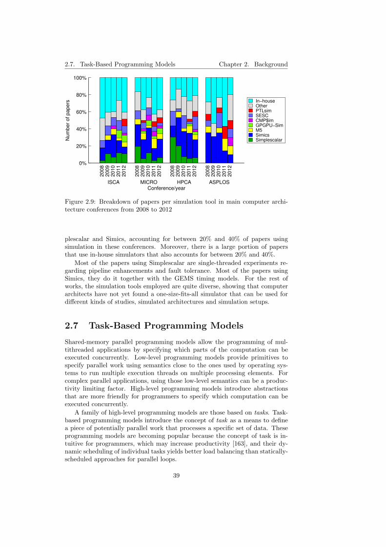
2.7. Task-Based Programming Models Chapter 2. Background
0%
20%
40%
60%
80%
100%
2008
2009
2010
2011
2012
2008
2009
2010
2011
2012
2008
2009
2010
2011
2012
2008
2009
2010
2011
2012
Num
ber
of papers
Conference/yearISCA MICRO HPCA ASPLOS
In−houseOtherPTLsimSESCCMP$imGPGPU−SimM5SimicsSimplescalar
Figure 2.9: Breakdown of papers per simulation tool in main computer archi-tecture conferences from 2008 to 2012
plescalar and Simics, accounting for between 20% and 40% of papers usingsimulation in these conferences. Moreover, there is a large portion of papersthat use in-house simulators that also accounts for between 20% and 40%.
Most of the papers using Simplescalar are single-threaded experiments re-garding pipeline enhancements and fault tolerance. Most of the papers usingSimics, they do it together with the GEMS timing models. For the rest ofworks, the simulation tools employed are quite diverse, showing that computerarchitects have not yet found a one-size-fits-all simulator that can be used fordifferent kinds of studies, simulated architectures and simulation setups.
2.7 Task-Based Programming Models
Shared-memory parallel programming models allow the programming of mul-tithreaded applications by specifying which parts of the computation can beexecuted concurrently. Low-level programming models provide primitives tospecify parallel work using semantics close to the ones used by operating sys-tems to run multiple execution threads on multiple processing elements. Forcomplex parallel applications, using those low-level semantics can be a produc-tivity limiting factor. High-level programming models introduce abstractionsthat are more friendly for programmers to specify which computation can beexecuted concurrently.
A family of high-level programming models are those based on tasks. Task-based programming models introduce the concept of task as a means to definea piece of potentially parallel work that processes a specific set of data. Theseprogramming models are becoming popular because the concept of task is in-tuitive for programmers, which may increase productivity [163], and their dy-namic scheduling of individual tasks yields better load balancing than statically-scheduled approaches for parallel loops.
39

2.7. Task-Based Programming Models Chapter 2. Background
Table 2.2: Task-based programming models
Programming Task Task Automaticmodel Nesting Dependencies Cut-offOmpSs [68] Yes Yes YesStarPU [19] Yes Yes NoThreading Building Blocks [144] Yes Yes NoOpenMP 3.1 [7] Yes No NoCilk [80] Yes No NoSequoia [77] Yes No NoX10 [57] Yes No NoChapel [55] Yes No NoCharm++ [101] No No No
Task-based parallel applications are partitioned into tasks that may exe-cute in parallel. A task is typically a function or a block of code and it isnot conceptually related to a specific execution thread. The runtime systemsoftware associated to the programming model assigns tasks to threads at runtime. This scheduling is dynamic and makes decisions based on the numberof threads and their availability. If a task needs to consume data produced byanother task, it waits for the producer task to complete using synchronizationprimitives that usually allow it to wait for a specific task or for all previouslycreated tasks. We refer to these scheduling and synchronization operations asparallelism-management operations or parops for short.
Table 2.2 shows a non-exhaustive list of programming models that supporttasks. All these programming models provide constructs in the form of specialkeywords, data structures or compiler directives to define tasks that will becreated at run time. Examples of these constructs for creating and synchroniz-ing tasks are shown in Figure 2.10. It shows parallel implementations of theFibonacci number recursive algorithm using three different programming mod-els from Table 2.2: OpenMP, Cilk and Threading Building Blocks. OpenMPmakes use of extended pragma annotations for tasks (in bold) and Cilk addsspecial keywords to the language (in bold). In both OpenMP and Cilk, fib(n-1)and fib(n-2) execute concurrently, and the calling task—fib(n)—waits for theircompletion on taskwait and sync respectively. Threading Building Blocks doesnot use language extensions and that results in a more complex piece of code.Threading Building Block’s spawn(b) creates task fib(n-2) asynchronously, andspawn and wait for all(a) creates task fib(n-1) and waits for both fib(n-1) andfib(n-2) to complete.
All the programming models in Table 2.2, but Charm++, support that taskscreate other tasks, which is referred to as task nesting. In Charm++, onlythe main thread creates tasks. Another feature of task-based programmingmodels is whether tasks are defined independent or have dependencies. OmpSs,StarPU and Threading Building Blocks support task dependencies by managinga task-dependency graph at runtime similar to the way a superscalar processormanages instruction dependencies. That is, if a task needs to consume datato be produced by other pending tasks, it waits and is not scheduled until itsdependencies are satisfied.
40

2.7. Task-Based Programming Models Chapter 2. Background
int fib(int n){
int i, j;if (n<2) return n;else {
#pragma omp task shared(i) firstprivate(n)i = fib(n-1);#pragma omp task shared(j) firstprivate(n)j = fib(n-2);#pragma omp taskwaitreturn i+j;
}}
(a) OpenMP
cilk int fib(int n){
if (n<2) return n;else {
int x, y;x = spawn fib(n-1);y = spawn fib(n-2);sync;return (x+y);
}}
(b) Cilk
long fib(int n) {int sum;FibTask& a = *new(task::allocate_root()) FibTask(n,&sum);task::spawn_root_and_wait(a);return sum;
}class FibTask: public task {public:
const int n;int* const sum;FibTask(int n_, int* sum_) :
n(n_), sum(sum_) {}task* execute() { // Overrides virtual function task::execute
int x, y;FibTask& a = *new(allocate_child()) FibTask(n-1,&x);FibTask& b = *new(allocate_child()) FibTask(n-2,&y);// Set ref_count to ‘two children plus one for the wait’set_ref_count(3);// Start b runningspawn(b);// Start a running and wait for all children (a and b)spawn_and_wait_for_all(a);// Do the sum
*sum = x+y;
return NULL;}
};
(c) Threading Building Blocks
Figure 2.10: Task-based implementation of the Fibonacci number recursive al-gorithm in (a) OpenMP 3.1, (b) Cilk and (c) Threading Building Blocks.
OmpSs also features a runtime-system mechanism to choose, at a task cre-ation point, whether it actually creates the task or if it executes the task se-quentially. This mechanism named cut-off [69] is useful when there are manypending tasks, all threads are busy and there is no need to open more paral-lelism, which would incur an unnecessary overhead. Cut-off can also be usedin other programming models, but it is the programmers responsibility to im-plement separate serial and parallel versions of the task and call either of themdepending on a user-defined heuristic. OmpSs provide this feature built-in, it
41
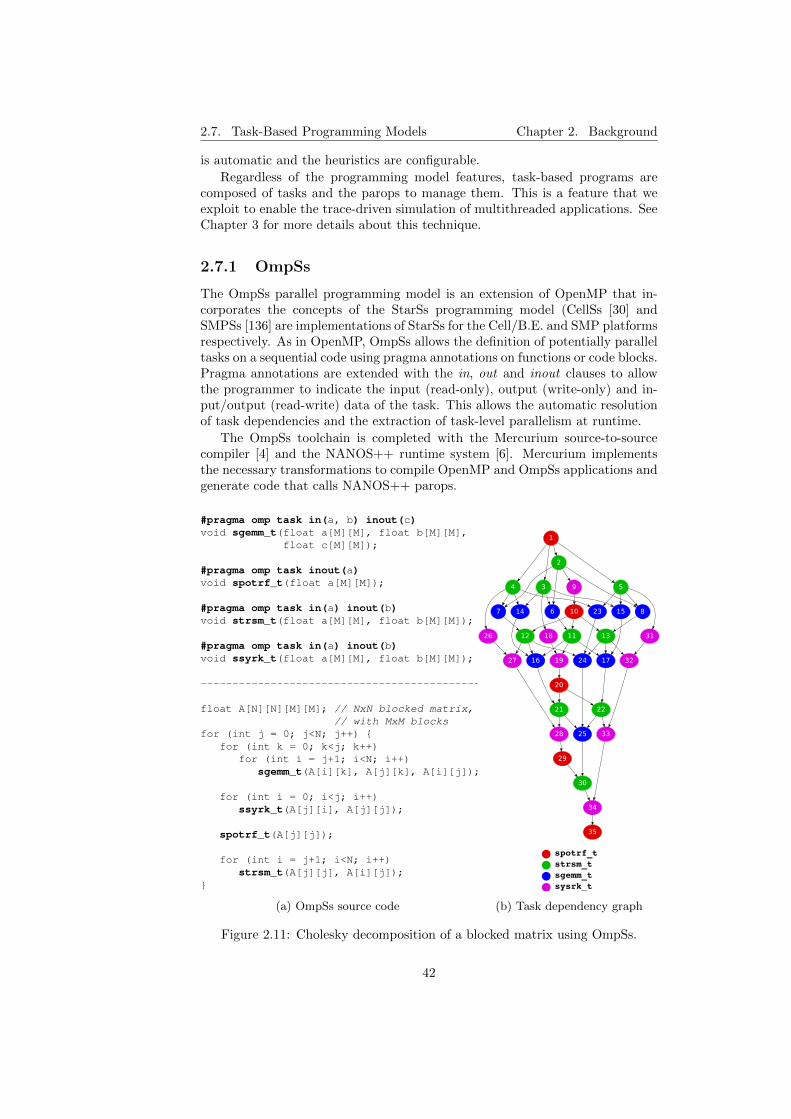
2.7. Task-Based Programming Models Chapter 2. Background
is automatic and the heuristics are configurable.
Regardless of the programming model features, task-based programs arecomposed of tasks and the parops to manage them. This is a feature that weexploit to enable the trace-driven simulation of multithreaded applications. SeeChapter 3 for more details about this technique.
2.7.1 OmpSs
The OmpSs parallel programming model is an extension of OpenMP that in-corporates the concepts of the StarSs programming model (CellSs [30] andSMPSs [136] are implementations of StarSs for the Cell/B.E. and SMP platformsrespectively. As in OpenMP, OmpSs allows the definition of potentially paralleltasks on a sequential code using pragma annotations on functions or code blocks.Pragma annotations are extended with the in, out and inout clauses to allowthe programmer to indicate the input (read-only), output (write-only) and in-put/output (read-write) data of the task. This allows the automatic resolutionof task dependencies and the extraction of task-level parallelism at runtime.
The OmpSs toolchain is completed with the Mercurium source-to-sourcecompiler [4] and the NANOS++ runtime system [6]. Mercurium implementsthe necessary transformations to compile OpenMP and OmpSs applications andgenerate code that calls NANOS++ parops.
#pragma omp task in(a, b) inout(c)void sgemm_t(float a[M][M], float b[M][M],
float c[M][M]);
#pragma omp task inout(a)void spotrf_t(float a[M][M]);
#pragma omp task in(a) inout(b)void strsm_t(float a[M][M], float b[M][M]);
#pragma omp task in(a) inout(b)void ssyrk_t(float a[M][M], float b[M][M]);
--------------------------------------------
float A[N][N][M][M]; // NxN blocked matrix,// with MxM blocks
for (int j = 0; j<N; j++) {for (int k = 0; k<j; k++)
for (int i = j+1; i<N; i++)sgemm_t(A[i][k], A[j][k], A[i][j]);
for (int i = 0; i<j; i++)ssyrk_t(A[j][i], A[j][j]);
spotrf_t(A[j][j]);
for (int i = j+1; i<N; i++)strsm_t(A[j][j], A[i][j]);
}
(a) OmpSs source code
1
2
34 5
67 8
9
14 15
18
23
26 311112 13
10
16 1719 2427 32
21 22
20
2528 33
30
29
34
35
spotrf_tstrsm_tsgemm_tsysrk_t
(b) Task dependency graph
Figure 2.11: Cholesky decomposition of a blocked matrix using OmpSs.
42

2.7. Task-Based Programming Models Chapter 2. Background
Figure 2.11 shows an example of an application written in OmpSs. Theapplication is a Cholesky decomposition of a blocked matrix. Figure 2.11a showsthe source code including the task definitions (top) using pragmas including theirin (read-only), out (write-only) and inout (read-write) task data dependencies.The task-generating code (bottom) executes sequentially creating new tasksat every function call. Figure 2.11b shows the task dependence graph of anexecution of the Cholesky decomposition on a 5x5 blocked matrix. The graphshows tasks as nodes, and inter-task dependencies as the edges interconnectingnodes. Different colors correspond to different task types and the node numbersshow the task creation order.
43

2.7. Task-Based Programming Models Chapter 2. Background
44

Chapter 3
Simulating MultithreadedApplications Using Traces
In this chapter we introduce our approach to enable the simulation of dynamically-scheduled multithreaded application using traces.
First, we explain the problem of capturing the behavior of a mulithreadedapplication in a trace and then trying to reproduce that behavior in a trace-driven simulation. Then, we cover the state of the art in this matter., which islimited to statically-scheduled applications.
We introduce a simulation methodology to address the problem for dynamically-scheduled applications. We also explain our implementation of this methodologyand show some experiments that prove its feasibility and usefulness. Finally, wediscuss the coverage and limitations of our approach and the research opportu-nities it opens for trace-driven simulation.
3.1 Problem
Multithreaded applications are parallel applications where all parallel executionstreams access data in a common address space. These applications are writ-ten using shared-memory parallel programming models. As mentioned in Sec-tion 2.7, regardless of the programming model, multithreaded applications con-sist of user code and parallelism-management operations. The user code is thepart of the application that defines its intrinsic behavior regardless of whetherthe application is executed in parallel or not. The parallelism-management op-erations, or parops for short, is the part of the code that manages the synchro-nization of multiple threads and schedules work to be executed concurrently.
One of the properties of trace-driven simulation is that the application be-havior is statically captured in a trace file and does not change during thesimulation of multiple machine configurations. This is a problem for simulat-ing multithreaded applications due to the dynamic behavior caused by timing-dependent operations. The behavior of a timing-dependent operation changesfor different machine configurations, something that a trace-driven simulatorcan not reproduce.
Figure 3.1 shows the execution of a multithreaded application with a mutualexclusion. Dashed lines mark the user code execution that is split in several
45
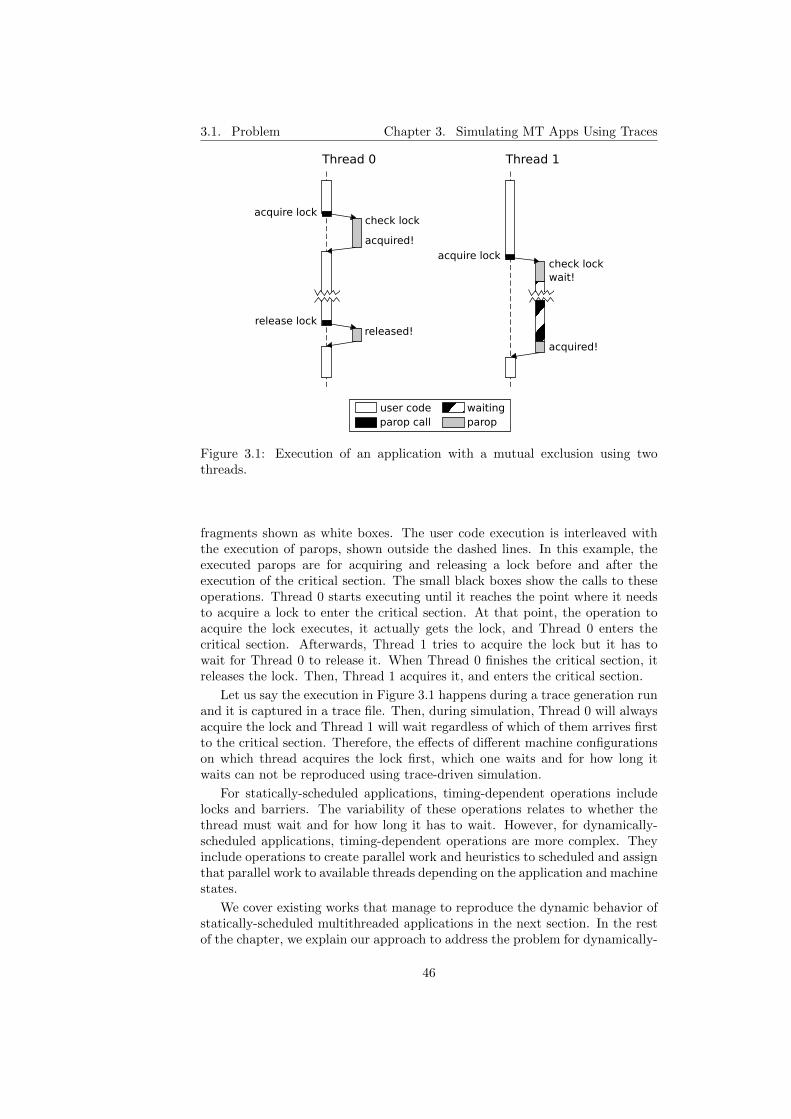
3.1. Problem Chapter 3. Simulating MT Apps Using Traces
Thread 0
acquire lockcheck lock
acquired!
release lockreleased!
Thread 1
acquire lockcheck lockwait!
acquired!
paropuser codeparop call
waiting
Figure 3.1: Execution of an application with a mutual exclusion using twothreads.
fragments shown as white boxes. The user code execution is interleaved withthe execution of parops, shown outside the dashed lines. In this example, theexecuted parops are for acquiring and releasing a lock before and after theexecution of the critical section. The small black boxes show the calls to theseoperations. Thread 0 starts executing until it reaches the point where it needsto acquire a lock to enter the critical section. At that point, the operation toacquire the lock executes, it actually gets the lock, and Thread 0 enters thecritical section. Afterwards, Thread 1 tries to acquire the lock but it has towait for Thread 0 to release it. When Thread 0 finishes the critical section, itreleases the lock. Then, Thread 1 acquires it, and enters the critical section.
Let us say the execution in Figure 3.1 happens during a trace generation runand it is captured in a trace file. Then, during simulation, Thread 0 will alwaysacquire the lock and Thread 1 will wait regardless of which of them arrives firstto the critical section. Therefore, the effects of different machine configurationson which thread acquires the lock first, which one waits and for how long itwaits can not be reproduced using trace-driven simulation.
For statically-scheduled applications, timing-dependent operations includelocks and barriers. The variability of these operations relates to whether thethread must wait and for how long it has to wait. However, for dynamically-scheduled applications, timing-dependent operations are more complex. Theyinclude operations to create parallel work and heuristics to scheduled and assignthat parallel work to available threads depending on the application and machinestates.
We cover existing works that manage to reproduce the dynamic behavior ofstatically-scheduled multithreaded applications in the next section. In the restof the chapter, we explain our approach to address the problem for dynamically-
46
3.2. State of the art Chapter 3. Simulating MT Apps Using Traces
scheduled applications which, to the best of our knowledge, no other work hasdone before.
3.2 State of the art
In the 1980s and early 1990s, trace-driven simulation was widely-used in com-puter architecture research. The problem explained in the previous sectionalready applied at that time, but it was in the context of shared-memory mul-tiprocessors.
Goldschmidt and Hennessy [88] compared trace-driven simulation and binary-instrumentation-driven simulation in terms of accuracy for multithreaded appli-cations running on shared-memory multiprocessors. They conclude that trace-driven simulation is accurate as long as there are not timing dependencies,precisely the problem we explain in the previous section. In statically-scheduledapplications, they identify timing dependencies in locks and barriers. Then, tomodel the different behavior on different configurations, they include a lock orbarrier event in the trace. When the simulator finds one of those events, it em-ulates its behavior depending on the state of the simulated machine. An ad-hocimplementation of lock and barrier operations carries out the necessary busy-waiting loop iterations until the synchronization condition is satisfied. Thisassumes the implementation of all locks and barriers in the application is thesame. However, for dynamically-scheduled applications, they do not manage toisolate the synchronization and scheduling timing-dependent code and concludethat trace-driven simulation is inaccurate in such cases.
Other works [105, 82, 108] employ the same technique and, in all cases, theyonly consider statically-scheduled applications and use an ad-hoc implementa-tion for locks and barriers as done in Goldschmidt and Hennessy’s work. Arecent work [183] proposes the same technique for reproducing locks and barri-ers without citing any of the previous papers. Their novelty is the annotationof locks and barriers to force the same execution order as in the original trace-generation run to provide deterministic replay.
3.3 Methodology
We developed a simulation methodology [150] to properly reproduce the dy-namic behavior of dynamically-scheduled multithreaded applications during sim-ulation, and overcome the problem explained in Section 3.1. This methodologytargets runtime-managed multithreaded applications and is based on their struc-ture.
As mentioned in previous sections, multithreaded applications consist of usercode and parops. User code is generally timing independent. To illustrate thisconcept, let us define user code as a set of sequential sections. A sequentialsection is a piece of code that executes the same instructions and in the sameorder regardless of the machine configuration. This means that instruction i (insequential order) always executes after instruction i-1 and before instructioni+1. Examples of sequential sections are an iteration in an OpenMP parallelloop, a Cilk parallel routine and an OmpSs task.
47

3.3. Methodology Chapter 3. Simulating MT Apps Using Traces
Parops determine the order and timing in which sequential sections are ex-ecuted. These include, but are not limited to: thread management operations(creation/spawn/join), synchronizations (locks, barriers, point-to-point), paral-lel work scheduling, and transaction begin and commit in transactional memorysystems. These operations are timing dependent because the instructions theyexecute depend on the machine configuration and state.
As an example, the sequential code section of each thread in Figure 3.1maintains its timing-independent order regardless of being interleaved by theexecution of parops. However, the execution of the lock acquire parops actuallyvaries on the machine state, more precisely on the lock variable state: whetherit is free or busy.
Given these properties, our methodology establishes that user code is simu-lated using a trace-driven approach, and parops are executed at simulation timebased on the state of the simulated machine.
3.3.1 Tracing
The application instrumentation for trace generation is aware of the applica-tion structure instead of blindly recording the instruction stream. First, theinstrumentation detects the entry and exit points of sequential sections in orderto store each of them separately. At the same time, instead of capturing theexecution of parops, the instrumentation discards it and includes a parop callevent for each of them. The event is stored at the point where the parop wasexecuted, and includes all necessary information to reproduce its execution atsimulation time. For example, for a lock acquire operation, the event wouldinclude the address or identifier of the lock variable to synchronize with.
The information included in a trace file is:
• Information to feed the timing model for each sequential section separately.For example, list of instructions or memory accesses.
• Parop call events including the information to carry out their executionat simulation time.
Application traces are indexed to enable the individual access to the infor-mation of each sequential section. This allows a simulated thread to switch torun a new sequential section or resume the execution of a suspended one whenthe execution of a parop carries out some scheduling operation. In the examplein Figure 3.1, the corresponding trace would include the two sequential sections(denoted with the dashed line), and one event for each lock acquire and releasecalls (black boxes) including the lock identifier for each of them.
Using this tracing method, an application is fully represented in a singletrace, and it is not necessary to generate a trace for every number of threadsto be simulated. In other words, one trace is generated per application andis used to simulate the execution of that application over multiple machineconfigurations with different numbers of cores. This results in a significantreduction in required disk space and tracing time compared to the state-of-the-art approaches requiring a separate thread for every number of cores to besimulated.
48

3.3. Methodology Chapter 3. Simulating MT Apps Using Traces
3.3.2 Simulation Infrastructure
Having these traces, the simulation tool requires to access to an implementationof the required parops. In parallel programming models, parop implementationsare typically provided as part of a runtime system library. In our methodology,the programming model runtime system is integrated in the simulation infras-tructure and, in order to work as decoupled as possible, a clearly-defined inter-face is required to provide the necessary services to both the simulator timingmodel and the runtime system.
SimulatorRuntimeSystem
parallelism-managementoperations
Interface
simulated arch stateand actions
Figure 3.2: Simulation infrastructure scheme.
Figure 3.2 shows a scheme of the simulation infrastructure. It has threecomponents: the trace-driven simulation engine, the runtime system and theengine-runtime interface. The trace-driven simulation engine includes the sim-ulated architecture timing model and the front-end to read the application trace.The runtime system is the one associated to the programming model of the simu-lated application. The engine-runtime interface has two parts. The first (shownat the top of the interface box in the figure) exposes and interface to the runtimesystem parops for the simulation engine to invoke them at simulation time. Thesecond (shown at the bottom) are the architecture dependent operations thatthe runtime system requires for the execution of parops. An example of theseoperations is the creation and join of threads, such as fork/join in OpenMPparallel loops.
3.3.3 Simulation Process
A simulation using multithreaded application traces in this infrastructure runsas follows. The simulator begins the simulation of the starting thread in theapplication, commonly known as the main or master thread. All remainingtreads start idle. The simulator performs the timing simulation of the user codein the main thread until it reaches the first parop event in the trace. At thatpoint, the simulator invokes the parop execution in the runtime system throughthe runtime system interface. The corresponding parop is then executed basedon the state and characteristics of the simulated machine. This is different toapproaches using binary instrumentation, where functional simulation is basedon the host machine state and characteristics, and to traditional trace-driventechniques where parop execution depends on the state and characteristics ofthe machine where the trace was collected. As an example of our simulationadaptability, scheduling decisions carried out by our simulation infrastructure
49

3.4. Implementation Chapter 3. Simulating MT Apps Using Traces
are based on the number of cores of the simulated architecture, the core status(running/wait/idle), or the overall work load at a given point in simulation time.
Then, after dynamically simulating a given parop, simulated threads mayhave been assigned new sequential sections according to the runtime systemdecisions. Each simulated thread then proceeds with the timing simulation ofthe sequential section assigned to it. For instance, when a parallel Cilk functionis invoked, the corresponding parop is called. According to the Cilk work-firstscheduling policy, the calling thread switches to execute the parallel function,while the calling context is switched to an available thread, or suspended untilthere is one available. Using our methodology, the simulation proceeds in thesame way as in the real machine: it assigns the parallel-function sequentialsection to the calling thread, and the calling context is either assigned to anavailable simulated thread, or is suspended until some simulated thread becomesavailable. This operation is possible because different sequential sections arecaptured and stored separately in the trace file and can be accessed individuallyto be simulated by different threads in the simulated machine.
3.4 Implementation
We implemented the proposed methodology using the TaskSim trace-driven sim-ulator (see Section 2.2), and the OmpSs runtime system called NANOS++ [6](see Section 2.7.1). This implementation supports multithreaded applicationswritten in the programming models supported by NANOS++, which currentlyare OpenMP and OmpSs.
In this environment, the target applications are compiled using the Mer-curium source-to-source compiler. The resulting binary calls an instrumentedversion of NANOS++ that generates traces for TaskSim. The resulting tracesare simulated on TaskSim, and NANOS++ is used as the runtime system forthe execution of parops at simulation time.
3.4.1 Instrumentation
NANOS++ incorporates an instrumentation engine that can be used to gener-ate traces with a custom trace format via the implementation of plugins thatare dynamically loaded at runtime. For our implementation, we developed aNANOS++ plugin to capture the runtime events of interest and generate tracesfor TaskSim. Additionally to the captured events, instruction or memory accesstraces are generated using PIN [113]. Since all parops are encapsulated in theruntime system, the instrumentation captures all the necessary information forsimulation.
The user-code sequential sections in this environment correspond directly toNANOS++ tasks. The main execution thread, which is a sequential section initself, is treated as a NANOS++ task as well. In the rest of this section, werefer to sequential sections as tasks, and to the main-thread associated task asmain task.
Figure 3.3 shows an example of an OmpSs application and a scheme of thecorresponding trace. The application creates four tasks and passes a separatematrix block to each of them as an argument. Afterwards, the main task syn-chronizes with the four created tasks using the taskwait directive before printing
50

3.4. Implementation Chapter 3. Simulating MT Apps Using Traces
#pragma omp task inout(mat)void t1( float mat[N][N] );
#pragma omp task inout(mat)void t2( float mat[N][N] );
#pragma omp task inout(mat)void t3( float mat[N][N] );
#pragma omp task inout(mat)void t4( float mat[N][N] );
(a) Task definition code
float matrix[4][N][N];
int main( int argc, char* argv[] ){
//...t1( matrix[0] );//...t2( matrix[1] );//...t3( matrix[2] );//...t4( matrix[3] );//...
#pragma omp taskwait
//print matrix contents}
(b) Main task code
ApplicationTrace
mai
n ta
skta
sk 1
task
2ta
sk 3
task
4
main task traceCPU user_code, main0inscreate_task id_t1, inout(0x72480,16384)CPU user_code, main1inscreate_task id_t2, inout(0x76480,16384)CPU user_code, main2inscreate_task id_t3, inout(0x7a480,16384)CPU user_code, main3inscreate_task id_t4, inout(0x7e480,16384)CPU user_code, main4instask_waitCPU user_code, main5ins
task4 traceCPU user_code, t4ins
t4ins trace
...20: sub r15, r12, r1324: store r35, r15 (0x7e6a0)28: sub r3, r31, r42C: load r21, r7 (0x80a88)30: addi r3, r334: beq r3 (next_i: 7C)7C: mul r32, r8, r980: mul r33, r10, r1184: mul r34, r12, r138C: store r32, r17 (0x7f280)90: store r33, r18 (0x7f284)...
(c) Trace contents
Figure 3.3: OmpSs application example and its corresponding traces for theTaskSim – NANOS++ simulation platform.
the contents of the matrix.
A trace of each task instance is captured separately and includes all parop-call events as they originally occurred. In the main task, there is one paropevent per task creation (on each function call) and one parop event for thetaskwait synchronization. The information related to each parop call (functionarguments) is also included in the trace, so they can be properly re-executed atsimulation time. Each create task event includes the id of the created taskand the address, size and directionality (inout, see Section 2.7.1). Computationperiods between parops are specified as CPU events and include a pointer tothe associated instruction or memory-access trace. As an example, the traceof task t4 has one CPU event that points to an instruction trace includingall instructions executed by the task. As previously explained, all task eventtraces and all instructions or memory-access traces are indexed to be accessedindividually.
51

3.4. Implementation Chapter 3. Simulating MT Apps Using Traces
3.4.2 Runtime Integration
Figure 3.4 shows a scheme of the components of our implementation. Theinterface between TaskSim and NANOS++ is split in two parts: the runtimebridge and the architecture-depenedent operations. The runtime bridge exposesall necessary parops implemented in NANOS++. This allows TaskSim to invokethem every time it finds a parop-call event in the trace. The architecture-dependent operations allow NANOS++ to manage the simulated threads andto assign tasks for them to execute.
TaskSim NANOS++
create tasktask waitwait on data
RuntimeBridge
Arch-depoperations
execute taskstart/join
bindyield
Figure 3.4: Implementation scheme.
Figure 3.4 includes a list of the main parops and architecture-dependentoperations used in our implementation. The main parops exposed by the run-time bridge (shown alongside the corresponding NANOS++ function betweenparenthesis) are the following:
• create task (createWD): the calling task requests the creation of a newtask. It specifies the new task id and the input and output data identifiers(address and size) for dependence tracking. The new task may be submit-ted for execution in any thread, or the cut-off mechanism (see Section 2.7)may decide to execute it inline.
• task wait (waitCompletion): the calling task requests to wait for all itspreviously-created tasks to complete execution. No additional informationis required.
• wait on data (waitOn): the calling task requests to wait for the last pro-ducer of a specific piece of data to complete execution. It specifies thecorresponding data identifiers.
These operations cover the basic task functionality of OmpSs and OpenMPapplications.
Similarly, TaskSim exposes the simulated architecture to NANOS++ throughthe architecture-dependent operations. These architecture-dependent opera-tions allow NANOS++ to assign tasks to simulated threads and set their state(idle/running). This architecture-dependent part of the interface is implementedas a NANOS++ plugin (as it is done for the architecture-dependent operationsof different real machines) and includes the following operations (alongside thecorresponding NANOS++ function between parenthesis):
• execute task (switchTo/inlineWork): executes a task on the current thread.It can be done on a separate context (switchTo) or on the current context(inlineWork).
52

3.4. Implementation Chapter 3. Simulating MT Apps Using Traces
• start/join thread (start/join): starts/finishes a new thread.
• bind thread (bind): binds the current thread to a hardware simulatedthread.
• yield thread (yield): requests a thread to yield.
Additionally, other architecture-dependent operations provide support forexplicit data transfers on distributed shared memory architectures, such as sys-tems including local/scratchpad non-coherent memories (e.g., GPU, multimedia,Cell/B.E.).
For the aforementioned functions to work, a set of data structures repre-senting the several machine threads at the runtime-system layer needs to becreated at startup. The simulator engine calls the runtime system to initializethese data structures through the init runtime-bridge function with the suitabletarget architecture features, such as the number of cores and core types (in het-erogeneous scenarios). At this point, the runtime system starts and initializesthe generic data structures that are common for any underlying architecture.Then, in order to initialize the architecture-dependent data structures, it invokesthe implementation of the createThread architecture-dependent operation.
This pre-simulation procedure provides the runtime system with the neces-sary abstraction layer to represent the threads in the simulated architecture.Thanks to this fact, and the decoupling between the parops and the user code,no data needs to be stored in the trace; and, as a result, the data structuresresulting from the runtime system initialization are sufficient for the correctfunctioning of the previously-listed operations at simulation time.
During simulation, NANOS++ has the illusion of running on a real machine,so tasks are scheduled, executed and synchronized in the same way as in a realexecution on whatever architecture configuration is simulated.
To apply this methodology to other programming models, we need all paropsto be encapsulated in the runtime system. Then, how easy is to integrate theruntime system with the trace-driven simulator depends on how easy it is tosetup the interface between them. The runtime bridge, which follows the bridgesoftware pattern, is easy to program as long as there is a clear API for theavailable parops in the runtime. For the architecture-dependent operations, theease of implementation depends on how spread out are these in the runtimesystem code. In NANOS++, all architecture-dependent code is encapsulated ina separate library that can be loaded at runtime. Then, for our implementationwe just had to replace the architecture-dependent library of the real machineby one implementing the operations for TaskSim.
3.4.3 Simulation Example
Simulation starts by assigning the main task to one of the simulated threads.All other simulated threads start idle. A separate context (user-level thread) iscreated for each simulated thread, to provide NANOS++ with the illusion ofa multithreaded machine, even though TaskSim is running on a single thread.Then, whenever a simulated thread wants to call a parop, the simulator switchesto the context associated to that simulated thread before entering the runtimesystem execution.
53

3.5. Experiments Chapter 3. Simulating MT Apps Using Traces
create task t1
create task t2create task t3
create task t4
task wait
exec t1
exec t2
exec t3
exec t4
Thread 0 Thread 1
main task
main task
wait!
(a) Two threads
create task t1
create task t2create task t3
create task t4
task wait
exec t1
exec t2exec t3
exec t4
Thread 0 Thread 1 Thread 2 Thread 3
main task
wait!
main task
(b) Four threads
Figure 3.5: Scheme of a multithreaded application simulation that generates 4tasks and waits for their completion on two and four threads.
Figure 3.5 shows the simulation of the application in Figure 3.3, usingtwo (Fig. 3.5a) and four simulated threads (Fig. 3.5b). Having all simulatedthreads setup, Thread 0 starts the simulation of the main task until it encountersthe first create task event. Then, it calls the corresponding parop throughthe runtime bridge, which results in the creation of task t1 in NANOS++.Task t1 is then ready and is scheduled to Thread 1 that is idle. Later, themain task also creates t2, t3 and t4. These are executed by different threadsdepending on the available cores in both examples, following a breadth-firstscheduling policy. After creating the four tasks, Thread 0 finds a task waitevent. At that point in the example with four cores, all created tasks are al-ready running in other threads, so Thread 0 waits for their completion. In theexample with two cores, only t1 is running, so Thread 0 starts t2. Thread 1finishes t1, and then switches to t3 and later to t4. Thread 0 completes t2,and switches back to the main thread where it waits for t4 to complete.
This example shows how our simulation methodology allows the simulationof different hardware configurations using a single trace per application.
3.5 Experiments
In this section we show a set of experiments that demonstrate the feasibilityand usefulness of the presented methodology, using our implementation shownin the previous section.
The first experiment is the scalability evaluation of a blocked-matrix multi-plication where each matrix block is processed by an OmpSs task. The compu-tation is done using the sgemm function in the BLAS library [37]. Figure 3.6shows its scalability (speed-up with respect to the execution with 8 cores), la-beled as matmul.
As it can be seen, matmul performance does not scale beyond 32 cores. Theanalysis of the results showed that the bottleneck is the task generation rate in
54
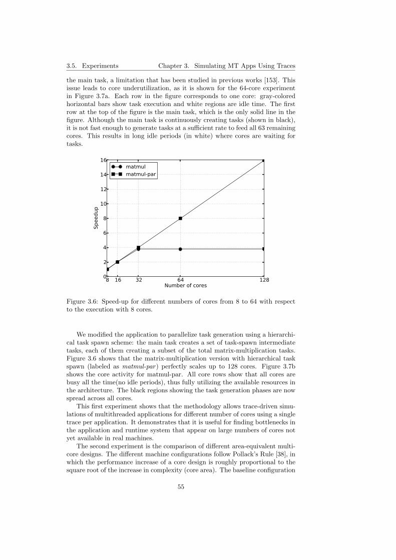
3.5. Experiments Chapter 3. Simulating MT Apps Using Traces
the main task, a limitation that has been studied in previous works [153]. Thisissue leads to core underutilization, as it is shown for the 64-core experimentin Figure 3.7a. Each row in the figure corresponds to one core: gray-coloredhorizontal bars show task execution and white regions are idle time. The firstrow at the top of the figure is the main task, which is the only solid line in thefigure. Although the main task is continuously creating tasks (shown in black),it is not fast enough to generate tasks at a sufficient rate to feed all 63 remainingcores. This results in long idle periods (in white) where cores are waiting fortasks.
8 16 32 64 128Number of cores
0
2
4
6
8
10
12
14
16
Spee
dup
matmulmatmul-par
Figure 3.6: Speed-up for different numbers of cores from 8 to 64 with respectto the execution with 8 cores.
We modified the application to parallelize task generation using a hierarchi-cal task spawn scheme: the main task creates a set of task-spawn intermediatetasks, each of them creating a subset of the total matrix-multiplication tasks.Figure 3.6 shows that the matrix-multiplication version with hierarchical taskspawn (labeled as matmul-par) perfectly scales up to 128 cores. Figure 3.7bshows the core activity for matmul-par. All core rows show that all cores arebusy all the time(no idle periods), thus fully utilizing the available resources inthe architecture. The black regions showing the task generation phases are nowspread across all cores.
This first experiment shows that the methodology allows trace-driven simu-lations of multithreaded applications for different number of cores using a singletrace per application. It demonstrates that it is useful for finding bottlenecks inthe application and runtime system that appear on large numbers of cores notyet available in real machines.
The second experiment is the comparison of different area-equivalent multi-core designs. The different machine configurations follow Pollack’s Rule [38], inwhich the performance increase of a core design is roughly proportional to thesquare root of the increase in complexity (core area). The baseline configuration
55

3.5. Experiments Chapter 3. Simulating MT Apps Using Traces
(a) matmul
(b) matmul-par
Figure 3.7: Snapshot of the core activity visualization of a blocked-matrix mul-tiplication a with 1 task-generation thread, and b with a hierarchical task-generation scheme
in this experiment includes 16 cores. Then we explore two alternatives: onewith four cores twice as fast, and another containing 64 cores with half theperformance each.
56

3.5. Experiments Chapter 3. Simulating MT Apps Using Traces
Figure 3.8 shows the speed-up with respect to the baseline configurationusing 16 cores. The results in the figure are shown for a set of scientific appli-cations programmed in OmpSs. A single trace per application is used for thesimulation of all hardware configurations. The configuration with four cores getsbetter performance for applications with less parallelism, as individual tasks willexecute faster and they do not get any benefit from having more cores avail-able. This is the case of pbpi and stap, which are limited by the performanceof the main task, and they do not scale to 16 cores. In this case, doubling thecore performance, doubles the overall application performance, as the sequentialbottleneck that dominates execution is completed twice as fast.
0.0
0.5
1.0
1.5
2.0
2.5
cholesky kmeans matmul matmul−par pbpi stap
Sp
ee
du
p
4 cores 2x16 cores 1x64 cores 0.5x
Figure 3.8: Application performance comparison for area-equivalent multi-coreconfigurations. Speed-up with respect to the 16-core baseline.
The configuration using 64 cores performs better for highly-parallel applica-tions, as the benefit of executing more tasks in parallel compensates the indi-vidual task performance loss. In our experiments, this applies to applicationsthat scale up to 64 cores, which is the case of matmul-par. For the rest of ap-plications, the baseline configuration is the best option. Cholesky, Kmeans andmatmul scale to 16 cores, so this configuration outperforms the one using justfour cores twice as fast. However, they do not scale to 64 cores, thus having anoverall performance loss due to the lower throughput of the individual cores.
For these experiments, our simulation framework required one trace per ap-plication and one simulation per configuration. The purpose of the experimentis twofold. First, to show the ability of our implementation to reproduce theapplications dynamic behavior for several configurations varying the number ofcores and the core type/performance. And, second, to show that the infrastruc-ture allows to get an insight of the reasons for application scalability on differentconfigurations.
57

3.6. Coverage Chapter 3. Simulating MT Apps Using Traces
3.6 Coverage
The proposed methodology covers multithreaded applications where timing-dependent code is decoupled from the application actual computation. Low-levelprogramming models (such as pthreads) allow the user to mix parops with usercode. Such applications would have to be modified so that parops are decoupledfrom user code, and parops can be exposed to the simulator. This needs to bedone for each parop and every application which is actually impractical. Thisresults in a limitation of the proposed methodology, that is directly inheritedfrom the mentioned weakness of low-level programming models.
Also, non-deterministic applications that rely on random values (such asMonte Carlo algorithms), include race conditions or depend on machine char-acteristics (e.g., data structures depend on number of cores) may not be re-producible during simulation. All required computation paths may have notexecuted on the original run, and thus are not available in the trace, making itstrace-driven simulation not doable.
Therefore, we have identified high-level programming models as the bestcases for our methodology. Since parops are fully provided in the associatedruntime system, user code and parops are decoupled. Therefore, the instrumen-tation of the runtime system covers the generation of traces for applications inthat programming model. Also, the runtime system of these programming mod-els can be directly used as the runtime system in the simulation platform, justby adding the corresponding architecture-dependent operations as explained inSection 3.4.
This simulation methodology opens several research opportunities that arenot practical using state-of-the-art trace-driven simulation.
First of all, new ideas on runtime system design, implementation and op-timization, such as new scheduling policies or more efficient management ofthread/task data structures, can be evaluated on future parallel architecturedesigns before the actual hardware is available. These evaluations are possiblethanks to the interface described in Section 3.3, which provides runtime sys-tems with the illusion of being executed on a real machine. Machines with largenumbers of homogeneous cores (64-128) accessing a shared memory are nowa-days available, although their cost is a limiting factor for its accessibility. Thepresented framework allows runtime system development for such large-scalemachines.
An interesting area of research is scheduling for heterogeneous architectures.The presented infrastructure allows the evaluation of runtime scheduling tech-niques for such heterogeneous on-chip architectures, which is not possible us-ing state-of-the-art trace-driven tools, and more difficult for execution-drivenapproaches as they may require a full compilation toolchain for the heteroge-neous simulated architecture sometimes requiring support for multiple ISAs.The trace-driven nature of our tools allows to have ISA-independent traces andjust needs to simulate the timing of the different core types.
Power-aware scheduling for large-scale architectures is another interestingresearch area, which is explorable using our methodology. Multithreaded ap-plications may trade off performance with power savings for non-critical coderegions, resulting in non-significant overall performance degradations. Analyz-ing those trade-offs is, again, not doable for models on existing trace-drivensimulators, and may be hard using measurements in real machines as the access
58

3.7. Summary Chapter 3. Simulating MT Apps Using Traces
to power sensors is in many cases limited (only a set of sensors are readable ata given point in time) or restricted (only available at the hypervisor level).
The presented methodology also provides dramatic reductions in the tracingtime and effort. A single trace represents the intrinsic behavior of the ap-plication, and it is not necessary to generate traces for different architectureconfigurations of the target parallel system. Applications are traced once, andused to evaluate many configurations. Also, there is no need to regenerate traceswhen there are changes in the runtime system. Whenever a new feature or op-timization is applied to the runtime system implementation, it is immediatelyavailable to the simulation framework, as the runtime system library is usedunchanged.
The time and effort required for tracing applications has been a major issuein research based on trace-driven simulation so far. Previous works had togenerate a separate traces per application and for each number of cores tobe simulated. Thus, by minimizing the required tracing time and effort, newmultithreaded applications can be quickly traced and incorporated as evaluationbenchmarks to research projects. Also, our methodology reduces the requireddisk space (a limitation explained in Section 2.3). This way, more applicationsor longer executions can be stored in the same disk space.
3.7 Summary
The simulation methodology presented in this chapter is, to the best of ourknowledge, the first hybrid methodology combining traces and execution forparallel application simulation. Traces are generated for the timing-independentuser code, and parops are re-executed at simulation time.
One of the contributions of this methodology is a significant reduction in theeffort for generating traces and disk space requirements. Multithreaded appli-cations are represented by a single trace, that can be used to evaluate multiplehardware configurations. Also, by using multithreaded applications written inhigh-level programming models, the instrumentation of the corresponding run-time system is enough to generate traces for any application.
The use of traces in our methodology provides all the benefits of trace-drivensimulation explained in Section 2.3. We showed simulations with up to 128 coresthat completed in a few minutes thanks to the lack of functional simulation andto raising the level of abstraction. More details about this can be found in thenext chapter.
59

3.7. Summary Chapter 3. Simulating MT Apps Using Traces
60
Chapter 4
Multiple Levels ofAbstraction
The techniques to reduce simulation time explained in Section 2.4 are useful toreduce the simulation time of cycle-accurate simulators. These simulators arefundamental tools for computer architecture research in order to understandthe workload stress on microarchitectural structures, but their time-consumingoperation limits their usability to exploring multi-cores with a few tens of cores.In general, cycle-accurate simulators are not suitable for simulating large-scalearchitectures, nor are they actually meant to be used for this.
Early high-level design decisions, or evaluations of the cache hierarchy, off-chip memory, or interconnect may not need such cycle-level understanding ofthe architecture, as microarchitecture decisions in those cases may be irrele-vant or even misleading. As it is widely suggested by the research commu-nity [180, 39], this fact opens the door to raising the level of abstraction ofthe core model. Furthermore, it allows to raise the level of abstraction of theapplication representation, as it does not necessarily have to be represented asan instruction stream. Most existing simulation tools are tied to this level ofapplication representation: execution-driven simulators need to work with theapplication instruction stream for functional simulation (see Section 2.3), as wellas trace-driven simulators that model the core pipeline.
In this chapter, we evaluate the implications of raising the level of abstractionof the simulation model by raising the level of abstraction of the simulatedapplication. We categorize simulation levels of detail and introduce a definitionof application abstraction levels. In this effort, we focus on the more abstract endof the spectrum, which is necessary for simulating large-scale architectures andwhere, to date, comparatively little work has been done. Based on the proposedapplication abstraction categories, we introduce two very high-level simulationmodes that are faster than functional simulaton, and that actually provide moreinsight. These are complemented with two more detailed simulation modes: onesimulating only memory accesses, and another working at the instruction level.We discuss and evaluate the utility and accuracy of these simulation models andanalyze their trade-offs between simulation speed and model detail compared tothe abstraction levels of popular simulators in computer architecture research.
61

4.1. State of the art Chapter 4. Multiple Levels of Abstraction
4.1 State of the art
The idea of variable-grain simulation detail is already present in the literatureand, in fact, many existing simulators offer several levels of abstraction withdifferent simulation speeds and levels of detail. Having different abstractionlevels is beneficial, not only due to having a faster (usually higher level) or moreaccurate simulation (usually lower level), but because each of them allows theresearcher to reason about certain aspects of the design.
The abstraction levels in many existing simulators range from microarchi-tectural pipeline modeling of, for example, in-order and out-of-order cores, tofunctional simulation. Examples are popular execution-driven simulators suchas Simplescalar [43], Simics [114] and gem5 [33]. These simulators provide asimulation mode for functional simulation, an intermediate mode that abstractsthe core pipeline and simulates the memory hierarchy in detail, and the mostdetailed mode that simulates both the memory hierarchy and the core pipelinein detail. We cover these simulation modes and their simulation speed andmodeling detail trade-offs in Section 4.4.
These aforementioned simulators target cycle-accurate simulation and theirdetail operation comes at the expense of simulation speed. However, other sim-ulators [128, 24, 164] use event-driven simulation and high levels of abstractionto achieve early design decisions and high-level insights for architectures whichcycle-accurate simulation is unfeasible.
An example of this kind of high-level computer architecture simulators isDimemas [24]. It models distributed-memory clusters with up to thousands ofcores, and its main target is parallel application analysis. Dimemas simulationsmainly focus on reflecting the impact of different cluster node configurations andinterconnection qualities on MPI communications. For this purpose it abstractsthe simulation of the cores assuming it has the same performance as in thetrace-generation machine (or a performance relative to it) and models MPIcommunication for a proper network contention simulation. A similar approachis followed by SMPI [63]. SMPI also models a cluster architecture, but the delayof MPI messages is calculated using an analytical model that considers not onlytransfer rates but also communication protocol delays.
Analytical models have also been used to abstract the model of the corepipeline. Interval simulation [83] is an approach in this direction. It uses asimple model that computes the IPC using an analytical model at intervals of agiven size. The analytical model assumes a fixed IPC based on the issue widthof the core and considers the IPC drop for an interval when there is a cachemiss or branch misprediction.
Another way of raising the level of abstraction is to abstract the simulatedmachine model while raising the level of abstraction of the application repre-sentation. We advocate for this approach, provide a definition of a hierarchyof levels of application abstraction and evaluate the corresponding simulatedmachine abstractions in the following sections. Previous simulators for tracememory simulation [35, 167, 138, 173, 105, 88, 109] use an application represen-tation at the memory level that considers memory accesses only.
In this chapter, we evaluate from the MPI-level abstraction used by Dimemas,to the memory level of trace memory simulators, and to the instruction levelused by execution-driven simulators. Also, we introduce a fourth abstractionlevel leveraged from our simulation methodology presented in Chapter 3.
62
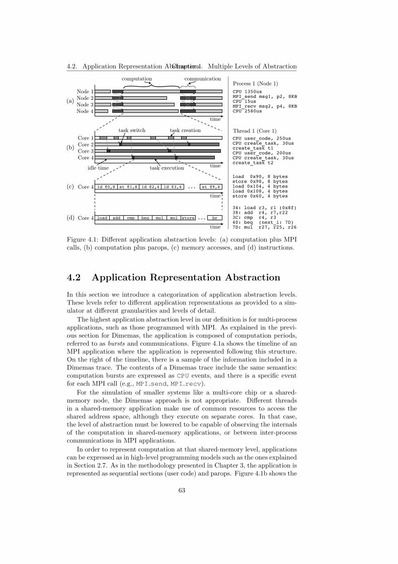
4.2. Application Representation AbstractionChapter 4. Multiple Levels of Abstraction
task switch
Node 1
Node 2
Node 3
Node 4
communicationcomputation
time
Core 1
Core 2
Core 3
Core 4
time
task creation
Core 4
time
ld @0,8 st @1,8 ld @2,4 ...
CPU 1350usMPI_send msg1, p2, 8KBCPU 15usMPI_recv msg2, p4, 8KBCPU 2580us
CPU user_code, 250usCPU create_task, 30uscreate_task t1CPU user_code, 200usCPU create_task, 30uscreate_task t2
load 0x90, 8 bytesstore 0x98, 8 bytesload 0x104, 4 bytesload 0x108, 4 bytesstore 0x60, 4 bytes
Process 1 (Node 1)
Thread 1 (Core 1)
(a)
(b)
(c)
task executionidle time
Core 4
time
load add cmp beq mul mul br...
34: load r3, r1 (0x8f)38: add r4, r7,r223C: cmp r4, r340: beq (next_i: 7D)7D: mul r27, r25, r26
store(d)
ld @3,4 st @9,4
Figure 4.1: Different application abstraction levels: (a) computation plus MPIcalls, (b) computation plus parops, (c) memory accesses, and (d) instructions.
4.2 Application Representation Abstraction
In this section we introduce a categorization of application abstraction levels.These levels refer to different application representations as provided to a sim-ulator at different granularities and levels of detail.
The highest application abstraction level in our definition is for multi-processapplications, such as those programmed with MPI. As explained in the previ-ous section for Dimemas, the application is composed of computation periods,referred to as bursts and communications. Figure 4.1a shows the timeline of anMPI application where the application is represented following this structure.On the right of the timeline, there is a sample of the information included in aDimemas trace. The contents of a Dimemas trace include the same semantics:computation bursts are expressed as CPU events, and there is a specific eventfor each MPI call (e.g., MPI send, MPI recv).
For the simulation of smaller systems like a multi-core chip or a shared-memory node, the Dimemas approach is not appropriate. Different threadsin a shared-memory application make use of common resources to access theshared address space, although they execute on separate cores. In that case,the level of abstraction must be lowered to be capable of observing the internalsof the computation in shared-memory applications, or between inter-processcommunications in MPI applications.
In order to represent computation at that shared-memory level, applicationscan be expressed as in high-level programming models such as the ones explainedin Section 2.7. As in the methodology presented in Chapter 3, the application isrepresented as sequential sections (user code) and parops. Figure 4.1b shows the
63
4.3. Model Abstraction Chapter 4. Multiple Levels of Abstraction
timeline of a task-based parallel application, which could also be part of an MPIapplication, as it occurs in the Roadrunner supercomputer [27] that features theCell/B.E. accelerator (see Section 2.1.1) and other systems featuring GPGPUs.As for Dimemas, computation bursts are expressed as CPU events, and areinterleaved with parops and, additionally, explicit memory transfer operationsfor distributed-memory multi-cores. In the example in Figure 4.1b, Core 1creates and schedules tasks (gray phases), and cores from 2 to 4 execute thosetasks (phases between dark gray) as they are being created by Core 1. Thisexample works as the one shown in Figure 3.5.
This level of abstraction is appropriate for quickly evaluating applicationscalability: whether an application can make use of an increasing numberof cores; and memory bandwidth requirements: whether data is transferredfast enough to cores to avoid slowdowns. For accelerator-based systems wherecomputation cores work on non-coherent scratchpad memories (e.g., Cell/B.E.,GPUs, DSPs), this abstraction level includes all information required for anaccurate evaluation of the memory system. Since such accelerators only ac-cess data in their scratchpad memories, the computation is not affected by theactivity in other components in the system. This means that, as long as theaccelerator core and scratchpad memory features remain unchanged, modifica-tions to the rest of the memory system and the interconnection network willnot affect the accelerator computation delay. Thus, modeling data transfers be-tween off-chip memory or last-level cache, and scratchpad memories is sufficientfor an accurate simulation. We demonstrate this point in Section 4.5.2.
However, for cache-based architectures this approach has, as is intended,some limitations in favor of simulation speed. The level of abstraction must belowered to simulate cache-based architectures accurately, so the memory systemis stressed with the application memory accesses. Figure 4.1c shows a list ofmemory accesses corresponding to a specific chunk of computation. This kindof representation is widely used by trace memory simulation methods [35, 167,138, 173, 105, 88, 109], some of them covered in Section 3.2.
Additionally, when it is necessary to explore microarchitectural issues con-cerning the core pipeline, or a more detailed understanding of the applicationexecution is required, the simulated application needs to be represented at theinstruction level. Figure 4.1d shows the list of instructions in a computationburst. This is the lowest level of representation of an application, and is the oneused in execution-driven simulators and trace-driven simulators focusing in thepipeline microarchitecture. As previously mentioned, this representation levelallows the detailed understanding of the microarchitecture activity, but preventsthe exploration of large-scale multi-cores due to its time-consuming operation.
4.3 Model Abstraction
The application abstraction levels shown in Figure 4.1 are the base for the archi-tecture model abstractions introduced in this section and that we implementedin TaskSim. To work with such application abstraction levels, we found appro-priate the use of event-driven simulation and the use of traces for all levels. Thisway, functional simulation is not needed at simulation time, and the applicationrepresentation can be actually abstracted beyond the instruction stream level.
The aforementioned application abstraction levels allow the definition of four
64
4.3. Model Abstraction Chapter 4. Multiple Levels of Abstraction
architecture model abstractions implemented in the following simulation modes:
• Burst: based on the shared-memory abstraction level (Fig. 4.1b). Ac-counts for the execution time of sequential sections and parop events.
• Inout: based on the shared-memory abstraction level (Fig. 4.1b). Extendsburst with explicit memory transfers.
• Mem: based on the memory abstraction level (Fig. 4.1c). Used for mem-ory simulation.
• Instr: based on the instruction abstraction level (Fig. 4.1d). Used forinstruction-level simulation.
The burst mode operates on a set of cores that simulate the computationbursts assigned to the associated threads, and carry out their synchronizationthrough the parops in the trace. Therefore, simulation of the memory systemand core pipeline is not necessary, so they are not even present on simulations inburst mode. However, for all other modes (inout, mem and instr), the cache hi-erarchy, network-on-chip and off-chip memory are simulated for a proper timingof memory accesses. More details on the implementation of these four architec-ture abstractions are given in the following sections.
4.3.1 Burst Mode
The burst mode implements a fairly simple event-driven core model. There isone trace for the main task, corresponding to the starting thread in the program,and then one trace for every other task executed in the application. A task traceincludes all computation bursts as CPU events, and the required parops for acorrect parallel execution. Since different tasks have separate traces, they canbe individually scheduled to available cores. The parallel work scheduling canbe either fixed or dynamic.
For fixed scheduling, as soon as a task is created and scheduled, any availablecore can start its execution. This mechanism is implemented using a semaphore-like strategy, that is signal and wait operations. After a task creation, a signalevent unblocks the execution of the corresponding task, which is assigned to acore as soon as it becomes free.
The same signal-wait mechanism allows the simulation of thread synchro-nizations such as task wait (waiting for all previously-created tasks), wait ondata (waiting for a producer task to generate a piece of data) and barriers.
The trace format for the burst mode using fixed scheduling includes thefollowing event types:
• CPU: indicates the beginning of a computation burst. It includes a com-putation type id and its duration in nanoseconds.
• Signal/Wait: used for thread synchronization. Both include a semaphoreid.
The core model using this trace format operates as follows. One of thesimulated cores starts simulation by reading the first event in the main tasktrace. CPU events are then processed by adding their duration to the current
65

4.3. Model Abstraction Chapter 4. Multiple Levels of Abstraction
cycle value in the target architecture (a ratio can be applied to burst durationsto simulate different core performance levels). The rest of the cores in thesystem start idle, and wait for tasks to be created and scheduled. Whenever aSignal event for task creation is found in the main task, any idle thread canstart simulating the corresponding task. The core taking the new task becomesactive, and starts processing its events.
For simulations using dynamic scheduling, TaskSim adopts the approachpresented in Chapter 3. The simulator employs an interface to a runtime systemthat executes the parops at simulation time. In this case, the Signal and Waitevent types are not necessary, and the trace includes, instead, the calls to theappropriate runtime system operations. When runtime call events are foundin the trace, the runtime system is invoked to execute them, and perform thecorresponding scheduling and synchronization operations. These operations areexecuted based on the state of the simulated machine, and task execution issimulated according to the decisions made by the runtime system. For moreinformation see Chapter 3.
4.3.2 Inout Mode
The inout mode builds on top of the burst mode to provide precise simulation ofmulti-core architectures using scratchpad memories (non-coherent distributedshared-memory systems). As previously mentioned, the execution of a coreaccessing a scratchpad memory is not affected by the features of other elementsin the system. The access to a scratchpad memory is deterministic, and thecore will only be delayed on eventual synchronizations with explicit memorytransfers between the scratchpad memory and the cache hierarchy levels, oroff-chip memory.
The trace format of the burst mode is enriched with specific events thatindicate the initiation of explicit memory transfers (e.g., DMA), and the syn-chronization with their completion before bursts reading that data:
• DMA: used to initiate an explicit memory transfer. It includes the transfertype (read/write), data memory address, size and a tag id.
• DMA wait: used to synchronize with previously initiated memory trans-fers. It includes a tag id.
The application simulation in inout mode works as in the burst mode but,when a DMA event is found, that core sends the proper commands to programthe memory transfer in the corresponding DMA engine. DMA transfers areasynchronous so the simulation of that memory transfer takes place in parallelwith the processing of computation bursts. Then, on a DMA wait event, the corestalls until it receives acknowledgement of the completion of the correspondingmemory transfer.
The core model in both burst and inout modes is intentionally simplistic.To avoid the slow detailed simulation of pipeline structures, the target coreis assumed to feature the same characteristics as the underlying machine onthe trace-generation run (or a relative performance using ratios for computa-tion bursts). Despite this simplicity, the isolation of computation on cores withscratchpad memories results in accurate memory system and interconnection
66

4.3. Model Abstraction Chapter 4. Multiple Levels of Abstraction
network evaluations that, for large target accelerator-based architectures, com-plete in a few minutes, as is shown in Section 4.5.2.
4.3.3 Mem Mode
For appropriately stressing the cache hierarchy elements and off-chip memoryon cache-based systems, the mem mode considers the list of executed memoryaccesses of the application. The burst mode is extended to add trace mem-ory simulation to the computation bursts in the target application. For eachcomputation burst, a trace of all corresponding memory accesses is capturedand a pointer to the resulting memory access trace is included in the associatedCPU event. Then, during simulation, when the simulator processes a CPU event,it ignores the computation burst duration in the trace, and it simulates thecorresponding memory access trace instead.
The trace formats of trace memory simulation works in the 80s and early90s, included just the memory accesses and, in some cases, the timestamp ofthe cycle when they were issued. However, in order to more precisely modelthe core performance, the memory access trace for the mem mode also includesthe number of non-memory instructions between memory accesses, thus leadingto a trace format analogous to the one of the TPTS simulator explained inSection 2.5.5. The records in the trace include the following information foreach memory access:
• Access type: Load or Store
• Virtual memory address.
• Access size in bytes.
• Number of instructions since the previous memory instruction.
The core model uses this information to simulate the performance of anout-of-order core by modeling the re-order buffer (ROB) structure; a techniqueby Lee et al. [109] also used in TPTS, and referred to as ROB OccupancyAnalysis. Using this method, simulation runs as follows. When the simulatedcore reaches a CPU event, it starts processing the associated memory accesstrace pointed by the event record. It reads the first memory access in thetrace, an starts issuing the previous instructions at a given issue rate. Whenall previous instructions are issued, the memory access is issued and sent to thefirst-level cache. Simulation keeps processing the following memory accesses inthe trace in the same manner, allowing several concurrent memory accesses inflight. However, to avoid performance overestimations and account for resourcehazards, simulation considers the limitation imposed by the ROB size. Thisassumes that the ROB is the main limiting factor in the core based on a studyby Karkhanis et al. [102]. For every memory access, the associated numberof previous instructions and the memory instruction itself, are stored in theROB. Then, when the ROB is full, no more trace records are processed, andonly the memory accesses in the ROB are allowed to be concurrently accessingthe memory system. Non-memory instructions in the ROB are committed ata given commit rate. Commit blocks when a pending memory access arrivesto the head of the ROB, and it does not unblock until the memory access isresolved.
67
4.3. Model Abstraction Chapter 4. Multiple Levels of Abstraction
This technique assumes that all memory references are independent. How-ever, for many applications, data dependencies may be the primary factor limit-ing memory-level parallelism. Memory access traces can be enriched with datadependencies and only allow independent accesses to be sent in parallel. Thisextension provides a closer approximation in terms of accuracy to instruction-level simulation.
This method is, in any case, faster than working at the instruction level, butwe further speed up simulation by applying trace stripping [138, 173] to TaskSimmemory access traces. This technique consists of simulating the memory accesstrace on a small direct-mapped filter cache, and only storing misses and thefirst store to every cache line (only required for the simulation of write-backcaches [173]). The resulting traces experience reductions in size of up to 98%depending on the application, and will perform the same number of misses asthe original trace on simulations of caches with a number of sets equal or largerto the number of sets of the filter cache. A limitation of this technique is thatthe cache line size of the simulated architecture must be the same that was usedin the filtering process for the filter cache.
The results in later sections show that this architecture model abstractionprovides a high simulation speed that is 18x faster than simulating at the instruc-tion level. We also evaluate this simulation mode in more detail in Chapter 5.
4.3.4 Instr Mode
In order to simulate core activity more accurately on systems with caches, theinstr mode extends the burst operation mode to allow the employment of in-struction traces for computation bursts, similarly to the extension applied for themem mode. The instruction stream is captured at tracing time using PIN [113],a dynamic binary instrumentation tool, and an instruction trace is generatedfor every computation burst. Then, as for the mem mode, the CPU event formatis extended to include an extra field for storing a pointer to the correspondinginstruction trace.
The core model in instruction mode operates exactly as in burst mode, butthe duration of CPU events is ignored, and the corresponding instructions aresimulated instead. There are many ways to encode an instruction trace but, ingeneral, they require to include the following information for every instruction:
• Operation code: it can be more or less generic depending on the targetISA and the detail of the core model (e.g., arithmetic rather than thespecific instruction opcode).
• Input and output registers.
• Memory address and data size for memory instructions.
• Next instruction for branch instructions.
This mode allows a detailed core simulation. Obviously, the more accuratethe core model, the longer the simulation takes to complete. In TaskSim, dif-ferent instruction-level core models can be used, and even switched from one toanother at simulation time, as described in the next section.
68

4.4. Speed-Detail Trade-Off Chapter 4. Multiple Levels of Abstraction
4.3.5 Summary
Table 4.1 shows a summary of the presented simulation modes. This includestheir applicability to different architecture types or software domains and theirusability for computer architecture studies. The burst mode allows to evaluateapplication scalability and, when it works integrated with a runtime system (asdescribed in Section 4.3.1), it also provides a framework to perform runtimesystem evaluations as we explained in Chapter 3. On top of these features, theinout mode allows to evaluate the memory system and interconnection networkdesigns, and it is accurate for scratchpad-based architectures. The mem modeprovides support for the evaluation of the memory system and interconnection,as well as the inout mode, and also allows to analyze the design of the cachehierarchy components. On top of this, the instr mode provides support forevaluating the microarchitecture of the core pipeline structures. Table 4.1 alsoshows an estimate of the simulation modes speed to give an idea of the trade-off between simulation speed and modeling detail. These trade-offs are morethoroughly evaluated in Section 4.4.
Table 4.1: Summary of TaskSim simulation modes. This includes their applica-bility on computer architecture evaluations, and their features also comparingto state-of-the-art (SOA) simulators
Mode Applicability FeaturesBurst Application scalability Potentially faster than native execution
RT system evaluation 100x faster than SOA functional sims
Inout Memory system 100-1000x faster than SOA instr.-level simsInterconnect Accurate for scratchpad-based CMPs
Mem Cache hierarchy 10-100x faster than SOA instr.-level sims
Instr Core microarchitecture –
It is worth mentioning that TaskSim allows to switch between different levelsof abstraction for different computation bursts along a single simulation. Thisis very useful to quickly traverse initial phases of an application in burst/inoutmode similarly to fast forwarding in some sampling-based simulation method-ologies (see Section 2.4.4), and then execute the computation bursts of interestin mem or instr mode.
4.4 Speed-Detail Trade-Off
We have chosen three of the most popular computer architecture research simu-lators to analyze their trade-offs between simulation speed and modeling detailfor their different levels of abstraction. The simulators are Simplescalar (seeSection 2.5.1), Simics and its timing module GEMS (see Section 2.5.2) andgem5 (see Section 2.5.3).
All three simulators are execution-driven, and thus rely on being providedwith the executable binary files of the application. This leads them to work
69
4.4. Speed-Detail Trade-Off Chapter 4. Multiple Levels of Abstraction
at the instruction level of abstraction (Figure 4.1d), but they still provide sev-eral levels of model abstraction, ranging from the highest level being functionalsimulation and, the lowest, the simulation of the core pipeline structures. Allabstraction levels in Simplescalar, Simics+GEMS and gem5 are compared tothe ones explained in the previous section in terms of simulation speed andmodeling detail. As a first observation, the instr level in TaskSim considers theapplication instruction stream as well, but mem, inout and burst benefit froma higher-level abstraction of the application representation to provide highersimulation speeds while still being insightful for different purposes.
Table 4.2 includes the different abstraction levels and performance of thesimulators considered in this study. The results were extracted from executionson an Intel Xeon running at 2.8 GHz, with 512 KB of L2 cache, 2 GB of DRAMat 1333 MT/s and running a 32-bit Linux distribution. For each application, werepeat the simulations four times, and took the fastest for all abstraction levelsto avoid operating-system noise. We simulated a single-core configuration in allsimulators because it is the fastest configuration in all cases. The addition ofsimulated cores usually leads to a super linear slowdown. We employed a setof scientific applications, listed in Table 4.4, for these experiments, all compiledwith gcc, -O3 optimization level and cross-compiled for PISA (Simplescalar),SPARC (Simics), Alpha (gem5) and x86 (TaskSim). The x86 binaries wereexecuted on the host system to generate traces for the different abstractionlevels of TaskSim.
The different abstraction levels of Simplescalar in this study are sim-fast,which just performs functional simulation supported by system-call emulation;sim-cache, which just simulates the first- and second-level caches with immediateupdate and a fixed latency for L2 cache misses (off-chip memory accesses);and sim-outorder, which adds to sim-cache the simulation of an out-of-orderprocessor pipeline. The three levels of abstraction correspond to the differentbinaries generated when compiling the Simplescalar distribution sources.
The highest abstraction level of Simics is its standalone execution (no timingmodules, -fast option) for functional simulation. The second level is the in-corporation of the GEMS Ruby module, set up for a MOESI CMP token config-uration; and the lowest level is the addition of the Opal module. We could havealso included an intermediate simulation setup including Opal but not Ruby.However, detailed modeling of core pipelines without a model for the memoryhierarchy does not provide any additional insight because other simulators donot have a configuration as such.
We configured gem5 to run in system-call emulation mode, and to sup-port the Alpha ISA. The different abstraction levels provide functional simu-lation (func: no flags are specified); the simulation of the cache system (cache:--caches --l2cache --timing); the addition to cache of an in-order corepipeline model (inorder : --caches --l2cache --inorder); and the addi-tion to cache of an out-of-order core pipeline model (ooo: --caches --l2cache--detailed). The TaskSim architecture model abstractions were discussed indepth in Section 4.3.
70

4.4.S
peed
-Detail
Tra
de-O
ffC
hap
ter4.
Mu
ltiple
Levels
ofA
bstraction
Table 4.2: Comparison of abstraction levels in existing simulators in terms of simulation speed and modeling detail
Abstraction level Speed (KIPS) Ratio to fastest Ratio to native Model detail
SIMPLESCALARsim-fast 20,425 1 288.07 functional onlysim-cache 5,946 3.43 999.29 sim-fast + cache hierarchy modelsim-outorder 1,062 19.23 5,669.55 sim-cache + OOO pipeline model
SIMICS + GEMSstandalone 32,517 1 128.23 functional onlyRuby 129 251.54 31,827.10 adds cache hierarchy and memory modelRuby + Opal 14 2,237.40 260,017.16 Ruby + OOO pipeline model
GEM5func 984 1 4,381.74 functional onlycache 401 2,45 10,734.61 adds cache hierarchy and memory modelinorder 47 20,92 98,335.57 cache + in-order pipeline modelooo 85 11,80 46,984.21 cache + OOO pipeline model
TASKSIMburst 4,175,762 1 0.80 computation bursts and paropsinout 132,573 31.50 25.70 burst + explicit memory transfersmem 2,067 2,020.32 1,561.27 burst + trace memory simulationinstr 113 36,919.01 31,173.21 burst + core pipeline model
71
4.4. Speed-Detail Trade-Off Chapter 4. Multiple Levels of Abstraction
The second column in Table 4.2 shows the simulation speed of the differentabstraction levels in kilo-instructions per second. The third column shows theratio of the simulation speed versus the fastest mode in the same simulator. Thevalues shown are the average for all applications. As expected, as the level ofabstraction is lowered, simulation gets slower. However, simulation speeds sig-nificantly vary between simulators due to their different simulation approaches:execution- vs. trace-driven, full-system vs. system-call emulation; and their dif-ferent levels of modeling detail. For example, Ruby, gem5 and TaskSim modelthe off-chip DRAM memory operation in detail, while Simplescalar applies justa fixed latency to L2 cache misses. The differences between the various func-tional modes of the execution-driven simulators are quite significant. Functionalsimulation in Simics is significantly faster than its other levels of abstraction dueto its software development target. Even though Simics simulates full-system, itis actually faster than sim-fast, whose model is much simpler. Contrarily, gem5functional mode is much slower even in system-call emulation mode as, in thiscase, the target is architecture simulation.
The abstraction levels modeling the core pipeline details, cache hierarchy andmemory system are the slowest in all simulators and their speed ranges from14 KIPS for Ruby+Opal, which implements a very detailed model, to 1062 KIPSfor Simplescalar which, apart from being not so complex, also benefits from sit-ting on a simple memory system model. It is remarkable that the inorder modelof gem5 is actually slower than the out-of-order model which, intuitively, shouldnot be the case, since an out-of-order core model is more complex. This fact hasbeen consistently found across different applications and different environmentsetups of gem5.
The forth column shows the ratio to the application execution on the hostmachine. It must be noticed that the comparison of simulation speed betweendifferent simulators does not match the comparison of their ratio to native ex-ecution. This is because different simulators employed binaries compiled fordifferent architectures that required different numbers of executed instructionsto complete.
It is worth highlighting that the TaskSim burst mode can be faster thannative execution, as was found for the applications in this study, and is 128xfaster than the fastest functional mode. This makes sense, as the speed of theburst mode depends on the number of events captured in the trace. In this case,the applications were compiled for task-parallel execution and simulated on asingle core, which is useful for the sake of comparison, but the burst mode is moreinteresting when simulating parallel systems, as is shown in the experiments inSection 4.5.1. The rest of the modes in TaskSim simulate the memory system,which slows down simulation in favor of simulation detail. The inout modebenefits from the aforementioned isolation of execution on accelerators to geta high simulation speed, only 25x slower than native execution, because onlyexplicit memory transfers are simulated. Finally, the mem mode provides an 18xspeedup compared to the instr mode. Among the rest of abstraction levels thatonly simulate the memory system, only sim-cache is faster, which, as previouslymentioned, uses a simple model for caches and does not simulate the off-chipmemory.
72
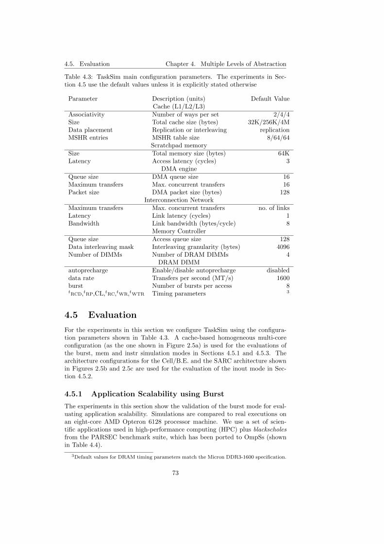
4.5. Evaluation Chapter 4. Multiple Levels of Abstraction
Table 4.3: TaskSim main configuration parameters. The experiments in Sec-tion 4.5 use the default values unless it is explicitly stated otherwise
Parameter Description (units) Default ValueCache (L1/L2/L3)
Associativity Number of ways per set 2/4/4Size Total cache size (bytes) 32K/256K/4MData placement Replication or interleaving replicationMSHR entries MSHR table size 8/64/64
Scratchpad memorySize Total memory size (bytes) 64KLatency Access latency (cycles) 3
DMA engineQueue size DMA queue size 16Maximum transfers Max. concurrent transfers 16Packet size DMA packet size (bytes) 128
Interconnection NetworkMaximum transfers Max. concurrent transfers no. of linksLatency Link latency (cycles) 1Bandwidth Link bandwidth (bytes/cycle) 8
Memory ControllerQueue size Access queue size 128Data interleaving mask Interleaving granularity (bytes) 4096Number of DIMMs Number of DRAM DIMMs 4
DRAM DIMMautoprecharge Enable/disable autoprecharge disableddata rate Transfers per second (MT/s) 1600burst Number of bursts per access 8tRCD,tRP,CL,tRC,tWR,tWTR Timing parameters 3
4.5 Evaluation
For the experiments in this section we configure TaskSim using the configura-tion parameters shown in Table 4.3. A cache-based homogeneous multi-coreconfiguration (as the one shown in Figure 2.5a) is used for the evaluations ofthe burst, mem and instr simulation modes in Sections 4.5.1 and 4.5.3. Thearchitecture configurations for the Cell/B.E. and the SARC architecture shownin Figures 2.5b and 2.5c are used for the evaluation of the inout mode in Sec-tion 4.5.2.
4.5.1 Application Scalability using Burst
The experiments in this section show the validation of the burst mode for eval-uating application scalability. Simulations are compared to real executions onan eight-core AMD Opteron 6128 processor machine. We use a set of scien-tific applications used in high-performance computing (HPC) plus blackscholesfrom the PARSEC benchmark suite, which has been ported to OmpSs (shownin Table 4.4).
3Default values for DRAM timing parameters match the Micron DDR3-1600 specification.
73
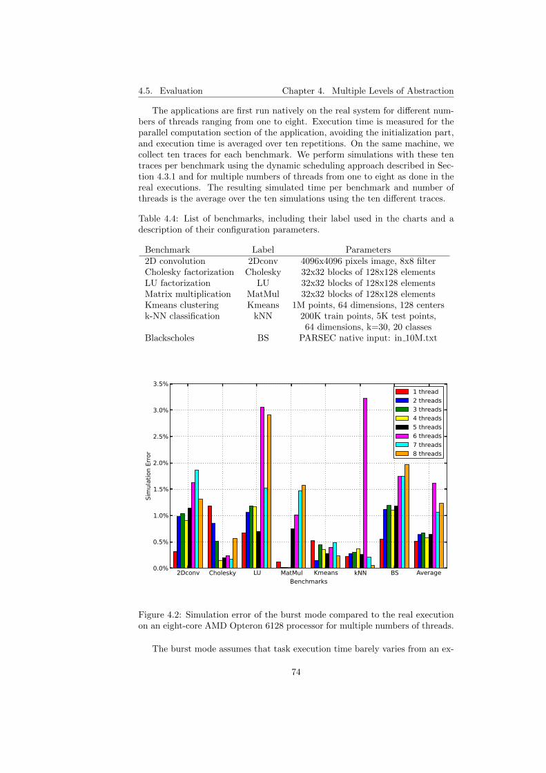
4.5. Evaluation Chapter 4. Multiple Levels of Abstraction
The applications are first run natively on the real system for different num-bers of threads ranging from one to eight. Execution time is measured for theparallel computation section of the application, avoiding the initialization part,and execution time is averaged over ten repetitions. On the same machine, wecollect ten traces for each benchmark. We perform simulations with these tentraces per benchmark using the dynamic scheduling approach described in Sec-tion 4.3.1 and for multiple numbers of threads from one to eight as done in thereal executions. The resulting simulated time per benchmark and number ofthreads is the average over the ten simulations using the ten different traces.
Table 4.4: List of benchmarks, including their label used in the charts and adescription of their configuration parameters.
Benchmark Label Parameters2D convolution 2Dconv 4096x4096 pixels image, 8x8 filterCholesky factorization Cholesky 32x32 blocks of 128x128 elementsLU factorization LU 32x32 blocks of 128x128 elementsMatrix multiplication MatMul 32x32 blocks of 128x128 elementsKmeans clustering Kmeans 1M points, 64 dimensions, 128 centersk-NN classification kNN 200K train points, 5K test points,
64 dimensions, k=30, 20 classesBlackscholes BS PARSEC native input: in 10M.txt
2Dconv Cholesky LU MatMul Kmeans kNN BS AverageBenchmarks
0.0%
0.5%
1.0%
1.5%
2.0%
2.5%
3.0%
3.5%
Simulation Error
1 thread2 threads3 threads4 threads5 threads6 threads7 threads8 threads
Figure 4.2: Simulation error of the burst mode compared to the real executionon an eight-core AMD Opteron 6128 processor for multiple numbers of threads.
The burst mode assumes that task execution time barely varies from an ex-
74

4.5. Evaluation Chapter 4. Multiple Levels of Abstraction
ecution on one thread compared to an execution on a higher number of threads.Therefore, codes optimized to fit task data in private caches and not being lim-ited by memory bandwidth are candidates to be accurately simulated, as it isthe case of highly-optimized HPC applications and scientific libraries. Figure 4.2shows the percent error of the predicted execution time using the burst modeand the execution on the real machine. The average error across all benchmarksand numbers of threads is below 1.6%, and the maximum error is 3.2%. Part ofthis error comes from the difference between the native and the trace-collectionruns and from instrumentation overheads.
Table 4.5: Cholesky factorization of a 4096×4096 blocked-matrix using differentblock sizes. The table shows the number of tasks, the average task executiontime and the comparison of real execution and simulation for four and eightthreads.
Block size 64× 128× 256× 512× 1024× 2048×64 128 256 512 1024 2048
Number of tasks 45760 5984 816 120 20 4Avg. task time 212µs 1.4ms 9.3ms 62ms 371ms 1.8s
Real vs. Simulation - 4 threadsReal exec. time (s) 2.89 2.12 2.01 2.19 3.26 7.43Predicted time (s) 2.65 2.12 1.98 2.14 3.13 7.38Error (%) 8.26 0.15 1.28 2.05 4.03 0.72Simulation time (s) 3.15 0.41 0.08 0.09 0.36 1.39Slowdown 1.09 0.20 0.04 0.04 0.11 0.19
Real vs. Simulation - 8 threadsReal exec. time (s) 1.56 1.08 1.05 1.35 3.06 7.41Predicted time (s) 1.34 1.07 1.02 1.28 3.02 7.38Error (%) 14.08 0.57 2.63 5.13 1.31 0.41Simulation time (s) 3.45 0.46 0.12 0.23 1.28 2.96Slowdown 2.21 0.48 0.11 0.17 0.42 0.40
We use Cholesky factorization (see Figure 2.11) as a case study of the valid-ity and usefulness of the burst mode for scalability analysis using multiple blocksizes (M×M in Figure 2.11a). Table 4.5 shows the number of tasks and averagetask execution time for multiple block sizes between 64×64 and 2048×2048. Weexecuted these multiple configurations in the real machine for different numbersof threads from one to eight and averaged the execution time over ten repeti-tions. We also simulated the same configurations using ten different traces andaveraged the predicted execution time.
Figure 4.3 shows the results. The configuration with 64×64 blocks shows anerror up to 14% because instrumentation overheads start becoming importantfor such small block sizes. However, for all other block sizes, simulation accu-rately reproduces real execution for multiple threads, even having collected thetrace on one thread. Table 4.5 shows the real and simulated execution times forfour and eight threads. The error for all block sizes except 64×64 tops at 5.2%.The results are not only accurate but also insightful. We can see that block sizeslarger than 512×512 do not exhibit enough parallelism to fully utilize all eightthreads. Block size 1024×1024 stops scaling at five threads, and 2048×2048
75

4.5. Evaluation Chapter 4. Multiple Levels of Abstraction
1 2 3 4 5 6 7 8 16 32 64128# threads
0
2
4
6
8
10
12
Exec
ution tim
e (s)
64x64 block size
realsimulation
1 2 3 4 5 6 7 8 16 32 64128# threads
0
2
4
6
8
10
12
Exec
ution tim
e (s)
128x128 block size
realsimulation
1 2 3 4 5 6 7 8 16 32 64128# threads
0
2
4
6
8
10
12
Exec
ution tim
e (s)
256x256 block size
realsimulation
1 2 3 4 5 6 7 8 16 32 64128# threads
0
2
4
6
8
10
12Ex
ecution tim
e (s)
512x512 block size
realsimulation
1 2 3 4 5 6 7 8 16 32 64128# threads
0
2
4
6
8
10
12
Exec
ution tim
e (s)
1024x1024 block size
realsimulation
1 2 3 4 5 6 7 8 16 32 64128# threads
0
2
4
6
8
10
12
Exec
ution tim
e (s)
2048x2048 block size
realsimulation
Figure 4.3: Comparison of real and simulated execution time for a 4096×4096blocked-matrix Cholesky factorization using multiple block sizes.
76
4.5. Evaluation Chapter 4. Multiple Levels of Abstraction
does not have any parallelism at all due to task dependencies.We extended the simulations for 16, 32, 64 and 128 threads. The results
show that block size 64×64 does not scale beyond 16 threads due to task cre-ation overheads, a problem we already explained for the matrix multiplicationexperiment in Section 3.5. That is that the rate at which the main threadproduces tasks is not fast enough compared to the rate at which tasks are exe-cuted by other threads, thus not being able to keep all threads busy. Block size512×512 stops scaling at 32 threads, and 256×256 has diminishing returns be-yond 16 threads, which makes the execution with blocks of 128×128 two timesfaster than with 256×256 when using 128 threads.
This kind of analysis is done fast because the burst mode is in most casesfaster than native execution. Table 4.5 shows the time required to simulate thefour and eight configurations on one thread (our implementation is not parallel),and the slowdown with respect to the real execution time. The average slowdownfor four threads is 0.28x (3.6x faster than native execution) and for eight threadsis 0.63x (1.6x faster).
4.5.2 Accelerator Architectures using Inout
In this section we introduce a set of experiments showing the utility and accuracyof the inout mode for architectures using scratchpad memories. Figure 4.4 showsseveral timelines of a Fast Fourier Transform (FFT) 3D application writtenin CellSs [30]. This FFT3D application is also compiled with the Mercuriumcompiler (see Section 2.7.1), but to use the CellSs runtime system.
Figure 4.4a is the real execution on a real Cell/B.E. Periods in gray representcomputation phases, and periods in black represent time spent waiting for datatransfers to complete. The application first performs an FFT on the first dimen-sion of a 3D matrix. FFT execution is computation-bound, so it is dominatedby computation time (gray). After the first FFT, it performs a transposition.The matrix transposition execution is memory-bound, so it is dominated bywaiting time (black). After the transposition, it performs another FFT but onthe second dimension, followed by a second transposition and, finally, anotherFFT on the third dimension. The five application stages are clearly identifiablein the timeline. The second transposition takes much longer than the first one,because data is accessed following a different pattern, which does not efficientlyuse the available off-chip memory bandwidth.
Figure 4.4b shows the timeline of the simulation in TaskSim using the inoutmode with a Cell/B.E. configuration (Figure 2.5b) and the fixed scheduling ap-proach as described in Section 4.3.1. The inout mode is able to closely reproducethe behavior of the real system. As it can be seen in Figure 4.4c, the same sim-ulation takes place but the off-chip memory data-interleaving granularity is setto 128 B instead of the default 4 KB in the real Cell/B.E. The time to completethe second transposition is then greatly shortened, resulting in a delay similarto that of the first transposition. This is because, using a 128 B interleavingscheme, several DIMMs are always accessed in parallel in both transpositions,thus achieving close to peak bandwidth efficiency, and getting a 30% reductionin total execution time.
In Figure 4.4d and Figure 4.4e, the same simulations (4 KB and 128 B inter-leaving granularities respectively) are carried out using a 256-core configurationof the SARC architecture (Figure 2.5c) excluding the L1 caches. Computa-
77
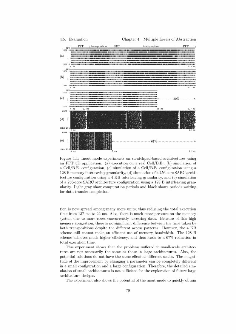
4.5. Evaluation Chapter 4. Multiple Levels of Abstraction
PPU
SPU 8
SPU 1
...
0 ms 135 ms
(a)
PPU
SPU 8
SPU 1
...(b)
(c)
PPU
SPU 8
SPU 1
...
(d)
(e)
CORE 1
CORE 256
...
CORE 1
CORE 256
...
0 ms 137 ms
0 ms 22 ms
0 ms 22 ms7 ms
0 ms 137 ms22 ms 95 ms
FFT FFT FFTtransposition transposition
30%
67%
Figure 4.4: Inout mode experiments on scratchpad-based architectures usingan FFT 3D application: (a) execution on a real Cell/B.E., (b) simulation ofa Cell/B.E. configuration, (c) simulation of a Cell/B.E. configuration using a128 B memory interleaving granularity, (d) simulation of a 256-core SARC archi-tecture configuration using a 4 KB interleaving granularity, and (e) simulationof a 256-core SARC architecture configuration using a 128 B interleaving gran-ularity. Light gray show computation periods and black shows periods waitingfor data transfer completion.
tion is now spread among many more units, thus reducing the total executiontime from 137 ms to 22 ms. Also, there is much more pressure on the memorysystem due to more cores concurrently accessing data. Because of this highmemory congestion, there is no significant difference between the time taken byboth transpositions despite the different access patterns. However, the 4 KBscheme still cannot make an efficient use of memory bandwidth. The 128 Bscheme achieves much higher efficiency, and thus leads to a 67% reduction intotal execution time.
This experiment shows that the problems suffered in small-scale architec-tures are not necessarily the same as those in large architectures. Also, thepotential solutions do not have the same effect at different scales. The magni-tude of the improvement by changing a parameter can be completely differentin a small configuration and a large configuration. Therefore, the detailed sim-ulation of small architectures is not sufficient for the exploration of future largearchitecture designs.
The experiment also shows the potential of the inout mode to quickly obtain
78
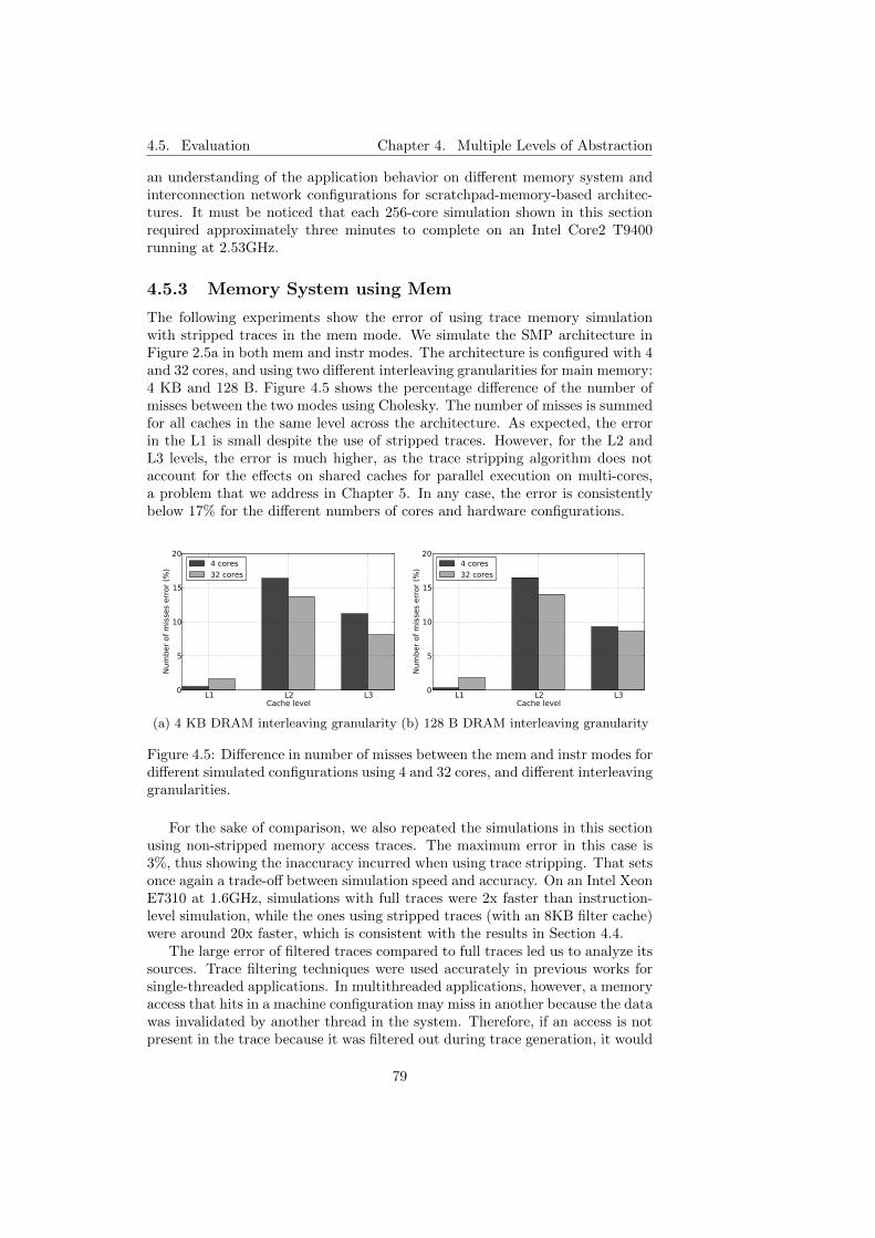
4.5. Evaluation Chapter 4. Multiple Levels of Abstraction
an understanding of the application behavior on different memory system andinterconnection network configurations for scratchpad-memory-based architec-tures. It must be noticed that each 256-core simulation shown in this sectionrequired approximately three minutes to complete on an Intel Core2 T9400running at 2.53GHz.
4.5.3 Memory System using Mem
The following experiments show the error of using trace memory simulationwith stripped traces in the mem mode. We simulate the SMP architecture inFigure 2.5a in both mem and instr modes. The architecture is configured with 4and 32 cores, and using two different interleaving granularities for main memory:4 KB and 128 B. Figure 4.5 shows the percentage difference of the number ofmisses between the two modes using Cholesky. The number of misses is summedfor all caches in the same level across the architecture. As expected, the errorin the L1 is small despite the use of stripped traces. However, for the L2 andL3 levels, the error is much higher, as the trace stripping algorithm does notaccount for the effects on shared caches for parallel execution on multi-cores,a problem that we address in Chapter 5. In any case, the error is consistentlybelow 17% for the different numbers of cores and hardware configurations.
L1 L2 L3Cache level
0
5
10
15
20
Num
ber o
f mis
ses
erro
r (%
) 4 cores32 cores
(a) 4 KB DRAM interleaving granularity
L1 L2 L3Cache level
0
5
10
15
20
Num
ber o
f mis
ses
erro
r (%
) 4 cores32 cores
(b) 128 B DRAM interleaving granularity
Figure 4.5: Difference in number of misses between the mem and instr modes fordifferent simulated configurations using 4 and 32 cores, and different interleavinggranularities.
For the sake of comparison, we also repeated the simulations in this sectionusing non-stripped memory access traces. The maximum error in this case is3%, thus showing the inaccuracy incurred when using trace stripping. That setsonce again a trade-off between simulation speed and accuracy. On an Intel XeonE7310 at 1.6GHz, simulations with full traces were 2x faster than instruction-level simulation, while the ones using stripped traces (with an 8KB filter cache)were around 20x faster, which is consistent with the results in Section 4.4.
The large error of filtered traces compared to full traces led us to analyze itssources. Trace filtering techniques were used accurately in previous works forsingle-threaded applications. In multithreaded applications, however, a memoryaccess that hits in a machine configuration may miss in another because the datawas invalidated by another thread in the system. Therefore, if an access is notpresent in the trace because it was filtered out during trace generation, it would
79

4.6. Summary Chapter 4. Multiple Levels of Abstraction
not be present during simulation to model a potential miss due to invalidations.This fact motived us to initiate research to enable more accurate simulationsof multithreaded applications using filtered traces. We present this work in thenext chapter.
4.6 Summary
In this chapter we have analyzed the use of multiple levels of abstraction in com-puter architecture simulation tools as a base for simulating large-scale architec-tures. As part of this analysis, we have characterized the levels of abstractionin existing simulation environments. In simulators requiring target applicationsto be represented as an instruction stream, the highest level of abstraction isfunctional emulation, which has been shown to be more than 100x slower thannative execution for the highly optimized Simics platform.
Also, we presented a definition of multiple application representations thatare more abstract than an instruction stream, and several simulation modesimplemented in TaskSim based on these representations. The two highest-levelmodes in TaskSim, burst and inout, have been shown faster than native exe-cution and 25x slower, respectively, while being more insightful than functionalsimulation. The burst mode has been proven useful and accurate for scalabilitystudies and application analysis, with an error below 8% compared to nativeexecution. Also, we tested the utility and accuracy of the inout mode for archi-tectures using scratchpad memories. The inout mode has been validated againsta real Cell/B.E., showing close performance behavior, and it is capable of sim-ulating up to 256-core configurations in less than three minutes. Finally, werevisit trace memory simulation techniques that are incorporated in TaskSimto provide an 18x speedup over instruction-level simulation with a maximumerror of 17% on the simulation of the cache hierarchy and memory system. Thiserror showed the inaccuracy inherent in using filtered traces for multithreadedapplications, which motives our work in the next chapter.
80

Chapter 5
Trace Filtering ofMultithreaded Applications
Recent works [108, 109] use trace memory simulation and trace filtering tech-niques such as trace stripping [138, 173] to reduce the simulation time of single-threaded configurations. These works generate a trace including all L1 missesof a benchmark running on a given microarchitecture. Then, they feed thistrace to a trace-driven simulator to explore the design space of the non-corecomponents, such as cache hierarchy—L2 and above—, off-chip memory andon-chip interconnect. This methodology assumes a fixed core microarchitectureand L1 cache for all trace-driven simulations. This is a significant limitation forsingle-thread/single-core analysis, as the non-core design space is limited. Thiskind of methodology seems more valuable for multi-core simulations where thenon-core design space is larger and a higher simulation speed is needed.
However, filtering a trace for multithreaded application simulations is notstraightforward. Trace stripping consists of filtering out all L1 hits and juststore L1 misses in the trace. This methodology assumes that for a given coremicroarchitecture and L1 cache configuration, the non-core accesses—to the L2cache—are independent of the non-core configuration. This is true for single-threaded applications where L1 accesses either hit or miss only depending onprevious accesses, which are always in the same order for a given core microar-chitecture. However, cache coherence operations in multi-core architectures,such as invalidations, may make an access to hit or miss depending on the otherthreads activities, which actually depend on the non-core configuration. In thisscenario, an access that was not recorded in the trace due to being assumedan L1 hit, may miss due to its data being invalidated by another cache in thesystem.
In this chapter, we introduce our approach to enable trace filtering for multi-threaded applications. First, we define the problem of filtering memory trace ofmultithreaded applications and explain what is the state of the art in this mat-ter. Then, we explain our methodology and our implementation using the memmode of TaskSim. Finally, we evaluate the method compared to the state of theart in terms of trace reduction, trace generation time, accuracy and simulationspeed-up.
81

5.1. Problem Chapter 5. Trace Filtering of MT Apps
5.1 Problem
Trace stripping [138] reduces trace size and simulation time by not includingL1 hits in the trace and only simulate L1 misses. Figure 5.1a shows a snippetof a memory access trace. The trace is passed through a direct-mapped cachethat informs for every access if it was a hit or a miss (Figure 5.1b). Every hitaccess is discarded and every miss is recorded in the trace giving as a result thefiltered trace in Figure 5.1c.
TYPE ADDRESS SIZE---- ------- ----LOAD 0x7ffff488 4LOAD 0x7ffff484 4LOAD 0x48fbc 8STORE 0x48e04 8LOAD 0x48f90 4LOAD 0x7ffff480 4LOAD 0x7ffff47c 4LOAD 0x7ffff478 4
(a) Original trace
TYPE ADDRESS SIZE---- ------- ----LOAD 0x7ffff488 4 (miss)LOAD 0x7ffff484 4 (hit)LOAD 0x48fbc 8 (miss)STORE 0x48e04 8 (miss)LOAD 0x48f90 4 (hit)LOAD 0x7ffff480 4 (hit)LOAD 0x7ffff47c 4 (miss)LOAD 0x7ffff478 4 (hit)
(b) Filter cache simulation
TYPE ADDRESS SIZE---- ------- ----LOAD 0x7ffff488 4LOAD 0x48fbc 8STORE 0x48e04 8LOAD 0x7ffff47c 4
(c) Filtered trace
Figure 5.1: Trace filtering: (a) example of a memory access trace, (b) how tracefiltering proceeds, and (c) the resulting filtered trace.
Let us say the filter cache is a 16 KB direct-mapped cache with 64-bytecache lines. In the filtering process, there are a series of cold, conflict andcapacity misses. The methodology states that both the full and filtered traceswill generate the same number of misses in caches with the same or largernumber of sets. Having more sets and/or a higher associativity (e.g., 64KB2-way set associative cache) will cause some of the capacity and conflict missesduring the filtering process to hit in simulation, but that will happen equally forthe full and the filtered traces, and in both cases the same accesses will miss.
The described methodology works in single thread scenarios because thereis a single order of accesses and there are no external events that may alter thecache state. However, in the case of a cache-coherent multi-core architecturerunning a multithreaded application, that is no longer the case. Some of theaccesses that hit during the filter process, may miss in a multi-core architecturebecause of cache coherence actions. Figure 5.2 shows two scenarios of the exe-cution of two threads in different simulation configurations that lead to differentthread interleavings. In both cases, a cache line invalidation occurs due to awrite in a remote cache to a shared cache line. In the case on the left, Thread 1executes Load D before Thread 0 executes Store B. Thus, D hits and the datain its cache gets invalidated afterwards. In the right case, Thread 0 executesStore B before, so Thread 1 misses on Load D as its cache line holding the datais invalid. The problem arises when the filtered trace is generated on the leftcase and D is filtered out. Then, if a given simulation configuration leads to theright case, D is not present in the trace because it is assumed a hit, and thesimulator cannot account for the timing effects of the cache miss.
Another characteristic of parallel programming models that may cause anaively filtered trace to fail is dynamic scheduling. The previous examples inFigure 5.2 assumed static scheduling. However, dynamically-scheduled parallelapplications may schedule pieces of work to different threads depending on the
82
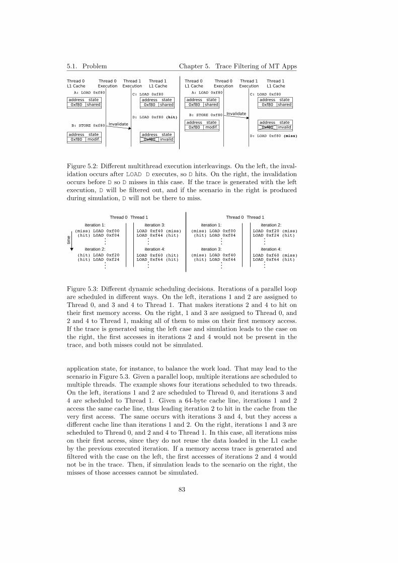
5.1. Problem Chapter 5. Trace Filtering of MT Apps
modif.0xf80address state
shared0xf80address state
shared0xf80address state
invalid0xf80address state
shared0xf80address state
modif.0xf80address state
Thread 0L1 Cache
Thread 1L1 Cache
Thread 0Execution
Thread 1Execution
A: LOAD 0xf80
shared0xf80address state
C: LOAD 0xf80
D: LOAD 0xf80 (hit)
B: STORE 0xf80 Invalidate
Thread 0L1 Cache
Thread 1L1 Cache
Thread 0Execution
Thread 1Execution
A: LOAD 0xf80 C: LOAD 0xf80
D: LOAD 0xf80 (miss)
B: STORE 0xf80 Invalidate
invalid0xf80address state
Figure 5.2: Different multithread execution interleavings. On the left, the inval-idation occurs after LOAD D executes, so D hits. On the right, the invalidationoccurs before D so D misses in this case. If the trace is generated with the leftexecution, D will be filtered out, and if the scenario in the right is producedduring simulation, D will not be there to miss.
Thread 0 Thread 1
iteration 1:(miss) LOAD 0xf00
iteration 2:(hit) LOAD 0xf20
iteration 3:LOAD 0xf40 (miss)
iteration 4:LOAD 0xf60 (hit)
(hit) LOAD 0xf04...
(hit) LOAD 0xf24...
LOAD 0xf44 (hit)...
LOAD 0xf64 (hit)...
time
Thread 0 Thread 1
iteration 1:(miss) LOAD 0xf00
iteration 3:(miss) LOAD 0xf40
iteration 2:LOAD 0xf20 (miss)
iteration 4:LOAD 0xf60 (miss)
(hit) LOAD 0xf04...
(hit) LOAD 0xf44...
LOAD 0xf24 (hit)...
LOAD 0xf64 (hit)...
Figure 5.3: Different dynamic scheduling decisions. Iterations of a parallel loopare scheduled in different ways. On the left, iterations 1 and 2 are assigned toThread 0, and 3 and 4 to Thread 1. That makes iterations 2 and 4 to hit ontheir first memory access. On the right, 1 and 3 are assigned to Thread 0, and2 and 4 to Thread 1, making all of them to miss on their first memory access.If the trace is generated using the left case and simulation leads to the case onthe right, the first accesses in iterations 2 and 4 would not be present in thetrace, and both misses could not be simulated.
application state, for instance, to balance the work load. That may lead to thescenario in Figure 5.3. Given a parallel loop, multiple iterations are scheduled tomultiple threads. The example shows four iterations scheduled to two threads.On the left, iterations 1 and 2 are scheduled to Thread 0, and iterations 3 and4 are scheduled to Thread 1. Given a 64-byte cache line, iterations 1 and 2access the same cache line, thus leading iteration 2 to hit in the cache from thevery first access. The same occurs with iterations 3 and 4, but they access adifferent cache line than iterations 1 and 2. On the right, iterations 1 and 3 arescheduled to Thread 0, and 2 and 4 to Thread 1. In this case, all iterations misson their first access, since they do not reuse the data loaded in the L1 cacheby the previous executed iteration. If a memory access trace is generated andfiltered with the case on the left, the first accesses of iterations 2 and 4 wouldnot be in the trace. Then, if simulation leads to the scenario on the right, themisses of those accesses cannot be simulated.
83

5.2. State of the Art Chapter 5. Trace Filtering of MT Apps
5.2 State of the Art
In the 1980s and early 1990s, there were several works to reduce the size ofmemory access traces for trace-driven memory simulation. This had two pur-poses: reducing the trace file size to make the most of the limited disk space,and reducing simulation time. Some works, such as Mache [156] and AE [107],just target to reduce trace file size and do not affect simulation time, althoughthey introduce an overhead to decompress (reconstruct) the trace. As an exam-ple, Mache recognizes different memory access streams during trace generation.Then, it records a tag and a base address for each stream, and just specifies thetag and the address difference for every subsequent access in that stream. Therationale behind this idea is that, in a 32-bit address space, specifying a tag andan address difference usually takes less bits than a full address.
Other works such as block filtering [15] both reduce trace size and improvesimulation performance, but they do it at the expense of simulation error.
The most interesting work for this thesis is trace stripping [138, 173]. It isinteresting because it reduces the trace file size, improves simulation speed, andit does not introduce simulation error. The only restriction is to use the samecache line size for the filter cache and the simulated caches. As explained in theprevious section, and shown in Figure 5.1, this method uses a direct-mappedcache as a filter cache. While generating the memory access trace, the accessesare passed to the filter cache, and only misses are recorded in the trace. In thework by Wang et al. [173], trace stripping is extended to simulate write-backcaches. In this case, not only are the filter cache misses recorded, but every firstwrite to a clean line is also included. This way, the access that may change thestate of a cache line to dirty is present in the trace and the corresponding writebacks take place during simulation.
A more recent work by Lee et al. [109] introduced a simulation methodologyto model not only the memory subsystem, but also a superscalar out-of-ordercore using traces and trace stripping. In this work, the trace is generated with acycle-accurate simulator from which they obtain a stripped (filtered) trace. Theypresent several models that use extra information in the trace such as the numberof instructions and/or cycles between memory accesses, and dependencies amongthem. Then, the trace is used to drive the simulation but replacing the core(including the L1 caches) by a trace player that sends memory accesses directlyto L2. The time and order in which accesses take place is decided consideringthe number of cycles between them, the size of the reorder buffer, and when theaccess is ready (its dependencies are satisfied).
All these previous works use trace filtering in the context of single-threadedapplications and multiprogrammed workloads. The only previous work thataddressed the use of trace filtering for simulating multithreaded applicationsis TPTS [108] (see Section 2.5.5). To address the problem explained in theprevious section, the authors present four alternatives:
• Naive filtering. Filter the multiple threads in the application as donefor single-threaded applications and ignore the effects of cache coherenceactions.
• Code region analysis. Disable filtering on code regions that accessshared data.
84
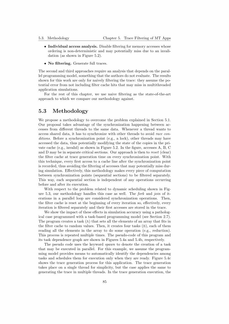
5.3. Methodology Chapter 5. Trace Filtering of MT Apps
• Individual access analysis. Disable filtering for memory accesses whoseordering is non-deterministic and may potentially miss due to an invali-dation (as shown in Figure 5.2).
• No filtering. Generate full traces.
The second and third approaches require an analysis that depends on the paral-lel programming model, something that the authors do not evaluate. The resultsshown for this work are only for naively filtering the trace: they assume the po-tential error from not including filter cache hits that may miss in multithreadedapplication simulations.
For the rest of this chapter, we use naive filtering as the state-of-the-artapproach to which we compare our methodology against.
5.3 Methodology
We propose a methodology to overcome the problem explained in Section 5.1.Our proposal takes advantage of the synchronization happening between ac-cesses from different threads to the same data. Whenever a thread wants toaccess shared data, it has to synchronize with other threads to avoid race con-ditions. Before a synchronization point (e.g., a lock), other threads may haveaccessed the data, thus potentially modifying the state of the copies in the pri-vate cache (e.g., invalid) as shown in Figure 5.2. In the figure, accesses A, B, Cand D may be in separate critical sections. Our approach is then to reset (clear)the filter cache at trace generation time on every synchronization point. Withthis technique, every first access to a cache line after the synchronization pointis recorded, thus avoiding the filtering of accesses that may potentially miss dur-ing simulation. Effectively, this methodology makes every piece of computationbetween synchronization points (sequential sections) to be filtered separately.This way, each sequential section is independent of any operations occurringbefore and after its execution.
With respect to the problem related to dynamic scheduling shown in Fig-ure 5.3, our methodology handles this case as well. The fork and join of it-erations in a parallel loop are considered synchronization operations. Then,the filter cache is reset at the beginning of every iteration so, effectively, everyiteration is filtered separately and their first accesses are stored in the trace.
We show the impact of these effects in simulation accuracy using a patholog-ical case programmed with a task-based programming model (see Section 2.7).The program creates a task (A) that sets all the elements of an array that fits inthe filter cache to random values. Then, it creates four tasks (B), each of themreading all the elements in the array to do some operation (e.g., reduction).This process is repeated multiple times. The pseudo-code of this program andits task dependence graph are shown in Figures 5.4a and 5.4b, respectively.
The pseudo code uses the keyword spawn to denote the creation of a taskthat may be executed in parallel. For this example, we assume the program-ming model provides means to automatically identify the dependencies amongtasks and schedules them for execution only when they are ready. Figure 5.4cshows the trace generation process for this application. The trace generationtakes place on a single thread for simplicity, but the case applies the same togenerating the trace in multiple threads. In the trace generation execution, the
85

5.3. Methodology Chapter 5. Trace Filtering of MT Apps
unsigned vec[SIZE];
//A writes vecvoid A() { for i=1..SIZE vec[i] = rand();}//B reads vecvoid B(int t) { for i=1..SIZE accum += vec[i];}
int main() { for 1..Nrepetitions spawn A(); for t=1..4 spawn B(t);}
A()
...
A()
A()
B(1) B(2) B(3) B(4)
B(1) B(2) B(3) B(4)
A( );
Thread 0
time
B(2);
B(2);
B(1);
B(3);
B(4);
B(4);
B(1);
B(3);
A( );
B(4);
B(2);
A( );B(1);
B(3);
...
A( );
Thread 0
time
A( );
A( );
Thread 1
A( );
A( );
A( );
Thread 2
A( );
Thread 3
B(1); B(2); B(3); B(4);
B(3); B(2); B(1); B(4);
B(2); B(1); B(4); B(3);
B(1); B(3); B(4); B(2);
B(2); B(1); B(4); B(3);
A( );B(4); B(2); B(1); B(3);
B(2); B(4); B(3); B(1);
...
...
...
...
b) Dependence grapha) Pseudo-code c) Trace generation
on one thread
d) Simulation on four threads
Figure 5.4: Pathological case. The figure shows: (a) the pseudo-code of theapplication; (b) the task dependence graph showing tasks in circles and thearrows between them are read-after-write (solid) and write-after-read (dashed)dependencies; (c) the execution in a single thread used for trace generation withthe order in which tasks are executed; and (d) the simulation of the applicationon four threads showing to which threads tasks are dynamically scheduled andtheir execution order.
first execution of A loads vec in the filter cache, say a 16 KB direct-mappedcache. Then, using the naive approach, the following executions of B and Ahit in the filter cache, so their accesses to vec are not recorded in the trace.Figure 5.4d shows a simulation using the application trace and modeling a four-thread multi-core architecture with private caches. Due to task dependencies,the simulation alternates the execution of A with the execution of the four in-stances of B. When the first A executes, it loads vec in Thread 0’s L1 cache.Then, the four instances of B execute in the four threads. In Thread 0 there isno error, as it hits as it did in trace generation; but the execution on Threads1, 2 and 3 find a cold cache where they should miss. However, the accesses inthe first execution of B(2), B(3) and B(4) are not present in the trace andthose misses are not simulated. The same happens in the second repetition. Aexecutes again in Thread 0, but its writes to vec are not present because theywere filtered out during trace generation, and the copies in the L1 caches ofThreads 1, 2 and 3 are not invalidated. Again, when Threads 1, 2 and 3 executethe second batch of B instances, their accesses to vec should miss, but againthey are not present in the trace because they also hit in the trace generationrun and were not recorded.
Using our methodology, the filter cache is reset at every spawn operationcall and task finalization during the trace generation run. Thus, before everyexecution of A and B, the filter cache is reset, and the first accesses to vec inevery task miss in the filter cache and are recorded in the trace. The simulationin Figure 5.4d using our methodology proceeds as follows. First, A loads vecin Thread 0’s L1 cache. Then, the several instances of B execute, and in allcases their first accesses to vec are simulated. B(1) reuses the data loadedby A and hits, but B(2), B(3) and B(4) find cold caches and they miss and
86

5.3. Methodology Chapter 5. Trace Filtering of MT Apps
load copies of vec to their private caches. After the first batch of B instancesexecute, a second A executes again in Thread 0. This invalidates vec’s copiesin the L1 caches of Threads 1, 2 and 3. Again, the first accesses to vec inthe following Bs are present in the trace, and they miss again, this time becausethose cached versions are invalid. This shows how our simple idea helps to builda filtered trace of a multithreaded application that is suitable for simulation ofa multi-core architecture.
We actually carried out these experiments with the implementation of ourmethodology explained later in Section 5.4. We coded this pathological case inOmpSs (see Section 2.7.1) and set it to run 500 repetitions of the main loop.The trace filtering process is as shown in Figure 5.4c: on one thread and using a16 KB direct-mapped filter cache with 64-byte lines. Using the naive approach,99.8% of the accesses get discarded, while using our methodology the filteringrate is 93.2%. The cache hit ratio of a sequential access pattern over four-byte consecutive elements that fit in cache is 93.75%: every cache line holds16 elements, so 1 out of 16 accesses to a cache line miss and the remaining 15hit. The filtering ratio of our methodology is on that range because the data isnot reused in the filter cache because it is cleared for every separate task. Thenaive approach gets a much higher filtering ratio, but may provide an erroneoussimulation as explained before.
20 50 100 150L2 cache latency
0.8
1.0
1.2
1.4
1.6
1.8
2.0
Norm
alized
Exe
cutio
n Time
fullresetnaive
Figure 5.5: Pathological case execution time normalized to full trace with L2cache latency of 20 cycles. A small L2 cache latency can be hidden by thesuperscalar core microarchitecture. Longer latencies delay L1 misses that arecorrectly simulated with our methodology (reset) and using the full trace. Thenaive method does not simulate those L1 misses, as they were filtered out duringtrace generation.
Figure 5.5 shows the normalized execution time of the naive method, la-beled naive; our proposal, labeled reset ; and the simulation using the full (non-filtered) trace, labeled full. We expect to have an underestimation of execution
87

5.4. Implementation Chapter 5. Trace Filtering of MT Apps
time using the naive method because it may not simulate some of the missesdue to invalidations and dynamic scheduling. The three methods are simulatedfor multiple L2 cache latencies on a multi-core configuration with five out-of-order cores: one core executes the main loop and creates tasks, and four coresexecute those tasks. This way we do not constraint the parallelism shown inthe dependence graph. For a latency of 20 cycles, the three methods predict thesame performance. Since vec fits in L2, the additional latency of an L1 missthat hits in L2 is hidden by the superscalar core model and does not stall thepipeline. However, when going to higher latencies, the core microarchitecturecannot hide that latency anymore and the full and reset configurations predicta higher execution time due to those L1 misses. However, the naive methoddoes not show this effect, as it cannot simulate those L1 misses: the accesseswere considered hits during trace generation, so they are not in the trace.
Alternatively to our methodology, a more complex application analysis couldbe done to identify only accesses to shared data and only avoid filtering those.However, this would require longer developments, should be done for every pro-gramming model to be supported, and trace generation may take significantlylonger. Also, such analysis would account only for potential invalidated data,but not for dynamic scheduling effects. Our methodology is simple, accountsfor both effects and is the same for multiple parallel programming models.
5.4 Implementation
As explained in previous chapters, multithreaded applications are composed ofsequential sections and parops. In Figure 5.6a we illustrate this concept foran OpenMP parallel loop. First, the application runs on one thread, whichis sequential section A. Then, the application executes a fork parop to spawna parallel loop and schedule its multiple iterations to the multiple availablethreads (four in this example). Then, every thread executes its share of theparallel loop, and each of the iterations is in itself a sequential section (B, C,D and E). After that, a join parop finalizes the parallel loop and continuesexecution on one thread.
Our methodology leverages this knowledge to effectively filter each sequen-tial section separately. This makes sense because the memory accesses in asequential section are always in the same order and their effects on the privateL1 cache state are always the same with respect to the previous and follow-ing accesses. To accomplish this, the trace generation engine must be notifiedwhenever a parop executes so it knows when to reset the filter cache.
The effort required to instrument parallel applications to catch parops dur-ing trace generation depends on the programming model. However, in general,all programming models provide a runtime system API (runtime library) and/orcompiler support for intermediate code generation. Figure 5.6b shows an ex-ample of the code generated by the GCC compiler for an OpenMP parallel forloop [2]. The programmer annotates the parallel loop with the pragma omp forkeywords, and the compiler transforms that construct to an intermediate codethat calls the libgomp OpenMP runtime library. Opposite to this, the pthreadsprogramming model exposes the API to the programmer, who then has to dealwith managing parallelism.
Some functions in a parallel programming model’s runtime system just pro-
88
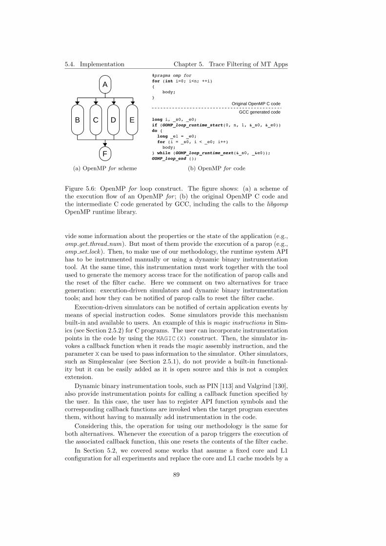
5.4. Implementation Chapter 5. Trace Filtering of MT Apps
A
B C D E
F
(a) OpenMP for scheme
#pragma omp for
for (int i=0; i<n; ++i)
{
body;
}
long i, _s0, _e0;
if (GOMP_loop_runtime_start(0, n, 1, &_s0, &_e0))
do {
long _e1 = _e0;
for (i = _s0, i < _e0; i++)
body;
} while (GOMP_loop_runtime_next(&_s0, _&e0));
GOMP_loop_end ();
Original OpenMP C code
GCC generated code
(b) OpenMP for code
Figure 5.6: OpenMP for loop construct. The figure shows: (a) a scheme ofthe execution flow of an OpenMP for ; (b) the original OpenMP C code andthe intermediate C code generated by GCC, including the calls to the libgompOpenMP runtime library.
vide some information about the properties or the state of the application (e.g.,omp get thread num). But most of them provide the execution of a parop (e.g.,omp set lock). Then, to make use of our methodology, the runtime system APIhas to be instrumented manually or using a dynamic binary instrumentationtool. At the same time, this instrumentation must work together with the toolused to generate the memory access trace for the notification of parop calls andthe reset of the filter cache. Here we comment on two alternatives for tracegeneration: execution-driven simulators and dynamic binary instrumentationtools; and how they can be notified of parop calls to reset the filter cache.
Execution-driven simulators can be notified of certain application events bymeans of special instruction codes. Some simulators provide this mechanismbuilt-in and available to users. An example of this is magic instructions in Sim-ics (see Section 2.5.2) for C programs. The user can incorporate instrumentationpoints in the code by using the MAGIC(X) construct. Then, the simulator in-vokes a callback function when it reads the magic assembly instruction, and theparameter X can be used to pass information to the simulator. Other simulators,such as Simplescalar (see Section 2.5.1), do not provide a built-in functional-ity but it can be easily added as it is open source and this is not a complexextension.
Dynamic binary instrumentation tools, such as PIN [113] and Valgrind [130],also provide instrumentation points for calling a callback function specified bythe user. In this case, the user has to register API function symbols and thecorresponding callback functions are invoked when the target program executesthem, without having to manually add instrumentation in the code.
Considering this, the operation for using our methodology is the same forboth alternatives. Whenever the execution of a parop triggers the execution ofthe associated callback function, this one resets the contents of the filter cache.
In Section 5.2, we covered some works that assume a fixed core and L1configuration for all experiments and replace the core and L1 cache models by a
89

5.4. Implementation Chapter 5. Trace Filtering of MT Apps
trace reader that sends memory accesses directly to the L2. In our methodology,however, the trace-driven simulator must include the L1 caches. Since we wantto account for cache coherent actions, such as invalidations, we need to maintainthe L1 cache state for those actions to take place. In the following section, wedescribe our implementation of this methodology to show its feasibility and asan example of how it can be put in practice.
5.4.1 Sample implementation
We implemented this methodology in the mem mode of TaskSim (see Sec-tion 4.3.3) and using the simulation methodology explained in Chapter 3. Weuse our NANOS++ instrumentation plug-in and PIN to generate traces at thememory level of abstraction (see Section 4.2). Figure 5.7 shows how the differentcomponents are combined to generate traces and carry out simulation. Two ver-sions of the OmpSs application binary are generated with Mercurium, one linkedto an instrumented version of NANOS++ (instrumented binary) and anotherone linked to a non-instrumented version (regular binary). The instrumentedbinary is run natively on one thread and it generates an application-level traceat the shared-memory abstraction level (see Section 4.2). The regular binary isexecuted with PIN, also in one thread, to catch all memory accesses. For thispurpose, we developed a PIN tool that generates the memory-access trace forthe instrumented application. If filtering is set in the PIN tool, the memoryaccesses are passed to a configurable filter cache that decides whether or not torecord them in the trace. Also, the NANOS++ API functions are registeredin our PIN tool to trigger the execution of callback functions to reset the filtercache, if filtering is enabled.
OmpSs.c
Mercurium
InstrumentedNANOS++
.so
InstrumentedOmpSsBinary
MercuriumOmpSsBinary
NANOS++.so
TraceGeneration
PIN Tool[filter/full]
Run
RunwithPIN
+ Full/filteredTrace
TaskSim
SimulationResults
Multi-coreModelConfig.
Figure 5.7: Trace generation and simulation process.
The result of the two runs is an application-level trace and one memory-access trace for every computation section. The two traces are combined to-gether to generate a single (full or filtered) trace for TaskSim.
The trace generation process (dashed line in the figure) is carried out by ourtrace reader/writer library, which is also used in TaskSim to read the input trace.
90

5.5. Evaluation Chapter 5. Trace Filtering of MT Apps
This helps to develop multiple core models based on a given trace semanticsregardless of the trace format as long as the API between the simulator and thetrace reader/writer is maintained.
5.5 Evaluation
In this section we evaluate our proposal using our implementation in terms ofincreased trace size, accuracy, trace generation cost and simulation time. Wecompare these metrics for three filtering approaches. The first is the state-of-the-art naive approach, labeled naive. As previously mentioned, it ignores cachecoherence actions and filters the trace without clearing the filter cache at anypoint. The second is our proposal, labeled reset, which clears the filter cachecontents on every synchronization point. And the third is the full/non-filteredmemory access trace, labeled full, which includes all memory accesses and is thebaseline in our experiments.
Parameter Description (units) Default ValueCore
Number of cores Number of cores in the chip 4/8/16Frequency Core/chip frequency (GHz) 1/2ROB size Number of ROB entries 64
L1 CacheAssociativity Number of ways per set 2Size Total cache size (bytes) 32KLatency Access latency (cycles) 2
L2 CacheAssociativity Number of ways per set 8Size Total cache size (bytes) 4MLatency Access latency (cycles) 20/50/100/150
Interconnection NetworkMaximum transfers Max. concurrent transfers no. of linksLatency Link latency (cycles) 1Bandwidth Link bandwidth (bytes/cycle) 8
Memory ControllerQueue size Access queue size 128Data interleaving mask Interleaving granularity (bytes) 4096Number of DIMMs Number of DRAM DIMMs 4
Off-chip Memorynumber of banks Number of banks per DIMM 8autoprecharge Enable/disable autoprecharge disableddata rate Transfers per second (MT/s) 1600burst Number of bursts per access 8tRCD,tRP,CL,tRC,tWR,tWTR Timing parameters 4
Table 5.1: TaskSim simulation parameters.
4Default values for DRAM timing parameters match the Micron DDR3-1600 specification.
91
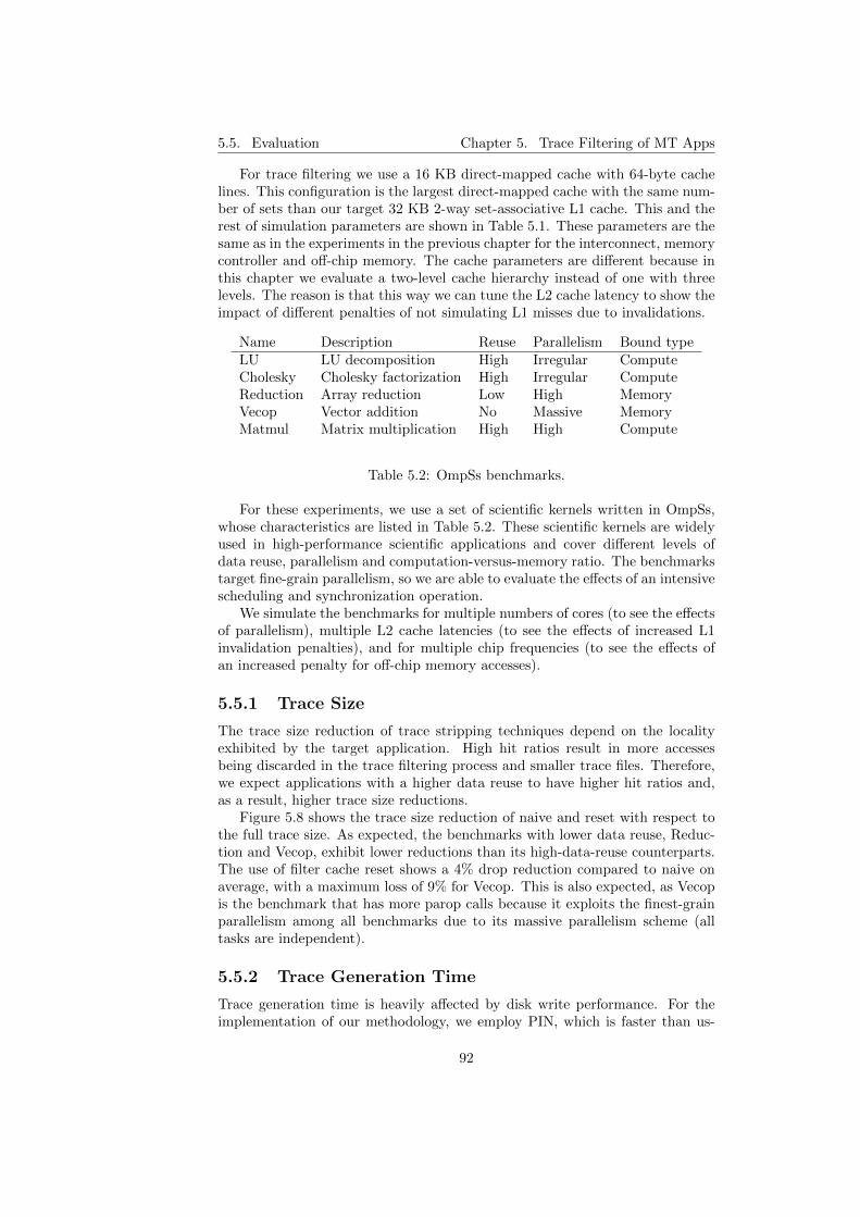
5.5. Evaluation Chapter 5. Trace Filtering of MT Apps
For trace filtering we use a 16 KB direct-mapped cache with 64-byte cachelines. This configuration is the largest direct-mapped cache with the same num-ber of sets than our target 32 KB 2-way set-associative L1 cache. This and therest of simulation parameters are shown in Table 5.1. These parameters are thesame as in the experiments in the previous chapter for the interconnect, memorycontroller and off-chip memory. The cache parameters are different because inthis chapter we evaluate a two-level cache hierarchy instead of one with threelevels. The reason is that this way we can tune the L2 cache latency to show theimpact of different penalties of not simulating L1 misses due to invalidations.
Name Description Reuse Parallelism Bound typeLU LU decomposition High Irregular ComputeCholesky Cholesky factorization High Irregular ComputeReduction Array reduction Low High MemoryVecop Vector addition No Massive MemoryMatmul Matrix multiplication High High Compute
Table 5.2: OmpSs benchmarks.
For these experiments, we use a set of scientific kernels written in OmpSs,whose characteristics are listed in Table 5.2. These scientific kernels are widelyused in high-performance scientific applications and cover different levels ofdata reuse, parallelism and computation-versus-memory ratio. The benchmarkstarget fine-grain parallelism, so we are able to evaluate the effects of an intensivescheduling and synchronization operation.
We simulate the benchmarks for multiple numbers of cores (to see the effectsof parallelism), multiple L2 cache latencies (to see the effects of increased L1invalidation penalties), and for multiple chip frequencies (to see the effects ofan increased penalty for off-chip memory accesses).
5.5.1 Trace Size
The trace size reduction of trace stripping techniques depend on the localityexhibited by the target application. High hit ratios result in more accessesbeing discarded in the trace filtering process and smaller trace files. Therefore,we expect applications with a higher data reuse to have higher hit ratios and,as a result, higher trace size reductions.
Figure 5.8 shows the trace size reduction of naive and reset with respect tothe full trace size. As expected, the benchmarks with lower data reuse, Reduc-tion and Vecop, exhibit lower reductions than its high-data-reuse counterparts.The use of filter cache reset shows a 4% drop reduction compared to naive onaverage, with a maximum loss of 9% for Vecop. This is also expected, as Vecopis the benchmark that has more parop calls because it exploits the finest-grainparallelism among all benchmarks due to its massive parallelism scheme (alltasks are independent).
5.5.2 Trace Generation Time
Trace generation time is heavily affected by disk write performance. For theimplementation of our methodology, we employ PIN, which is faster than us-
92
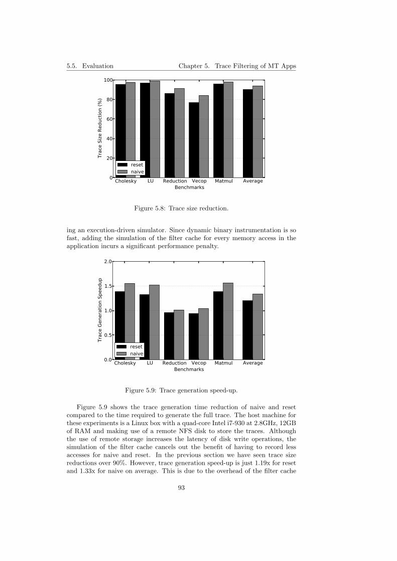
5.5. Evaluation Chapter 5. Trace Filtering of MT Apps
Cholesky LU Reduction Vecop Matmul AverageBenchmarks
0
20
40
60
80
100
Trac
e Si
ze R
educ
tion
(%)
resetnaive
Figure 5.8: Trace size reduction.
ing an execution-driven simulator. Since dynamic binary instrumentation is sofast, adding the simulation of the filter cache for every memory access in theapplication incurs a significant performance penalty.
Cholesky LU Reduction Vecop Matmul AverageBenchmarks
0.0
0.5
1.0
1.5
2.0
Trac
e Ge
nera
tion
Spee
dup
resetnaive
Figure 5.9: Trace generation speed-up.
Figure 5.9 shows the trace generation time reduction of naive and resetcompared to the time required to generate the full trace. The host machine forthese experiments is a Linux box with a quad-core Intel i7-930 at 2.8GHz, 12GBof RAM and making use of a remote NFS disk to store the traces. Althoughthe use of remote storage increases the latency of disk write operations, thesimulation of the filter cache cancels out the benefit of having to record lessaccesses for naive and reset. In the previous section we have seen trace sizereductions over 90%. However, trace generation speed-up is just 1.19x for resetand 1.33x for naive on average. This is due to the overhead of the filter cache
93

5.5. Evaluation Chapter 5. Trace Filtering of MT Apps
simulation. In our proposal, the process of resetting the filter cache implies anextra cost that makes trace generation longer than for the full trace in the mostmemory intensive benchmarks Reduction and Vecop.
In any case, trace generation is a one-time operation so, in most cases, itscost is not critical.
5.5.3 Simulation Accuracy
In this section we give a measure of how our proposal reduces the simulationerror of the state-of-the-art naive approach. Figure 5.10 shows the simulationerror introduced by trace filtering in both reset and naive having the full trace asthe baseline. The figure shows three charts, each of them for a different numberof simulated cores: four, eight and sixteen. At the same time, each chart isdivided in two halves: the left half is the configuration with 1 GHz cores, andthe right half for 2 GHz cores. The x-axis shows groups of L2 cache latencies,each group for a different benchmark. The L2 cache latencies are 20, 50, 100 and150 cycles, to be consistent with the experiment shown in Section 5.3. Althoughthe largest latencies are unrealistic, we want to show these extreme cases as anupper-bound of simulation error for trace filtering, where L1 misses have a largepenalty, even if the data is reused on chip (i.e., they hit in L2 cache). Also,these large penalties are closer to the effect of in-order cores. Our out-of-orderconfiguration is able to hide a 20-cycle latency, something an in-order core couldhardly hide.
We expected the results of reset to be closer to the simulation of the fulltrace. However, we have found quite a lot of variability during the simulationsdue to dynamic scheduling decisions (butterfly effect). Slight differences intiming due to filtering make tasks to be scheduled to different threads in thedifferent configurations which leads to completely different data reuse patternsin the private caches.
There are a few cases where our methodology has a larger error than naive.In most of these cases, apart from the variability inherent to dynamic scheduling,we have found the limitation of filtered traces to handle ping-pong effects dueto false sharing. This limitation is the same for both reset and naive, but dueto dynamic scheduling, reset missed more false sharing conflicts than naive inthe cases where reset has a larger error (the conflicting tasks were scheduled inthe same thread for naive, and to different threads in the same time frame forreset). The problem with false sharing is that, even if the first accesses to everycache line after a parop execution are recorded, consequent hit write accessesmay be accessing a cache line containing data written by another thread. Thethreads do not share the data, but both data reside in the same cache line thatis invalidated on every write. The full trace recreates correctly these scenarios,but filtered traces cannot because the accesses that may ping-pong are not inthe trace. A possible technique to handle this would be to avoid filtering writes,and only filter reads. However, this may be too aggressive so we think thatfurther investigation is needed for this purpose.
However, even considering these effects, our methodology consistently re-duces the simulation error incurred by the incorrect filtering of the naive method-ology. Figure 5.11 shows the average across all benchmarks and frequencies forthe different multi-core configurations. On average, reset halves the error ofnaive from 9% to 4.5%.
94

5.5. Evaluation Chapter 5. Trace Filtering of MT Apps
20 50 100
150 20 50 100
150 20 50 100
150 20 50 100
150 20 50 100
150 20 50 100
150 20 50 100
150 20 50 100
150 20 50 100
150 20 50 100
15030
25
20
15
10
5
0
5
Sim
ulat
ion
Erro
r (%
)
Cholesky LU Reduction Vecop Matmul Cholesky LU Reduction Vecop Matmul
resetnaive
1GHz 2GHz
L2 Cache Size/Benchmarks
(a) Simulation error for 4-core CMP
20 50 100
150 20 50 100
150 20 50 100
150 20 50 100
150 20 50 100
150 20 50 100
150 20 50 100
150 20 50 100
150 20 50 100
150 20 50 100
15030
25
20
15
10
5
0
5
Sim
ulat
ion
Erro
r (%
)
Cholesky LU Reduction Vecop Matmul Cholesky LU Reduction Vecop Matmul
resetnaive
1GHz 2GHz
L2 Cache Size/Benchmarks
(b) Simulation error for 8-core CMP
20 50 100
150 20 50 100
150 20 50 100
150 20 50 100
150 20 50 100
150 20 50 100
150 20 50 100
150 20 50 100
150 20 50 100
150 20 50 100
15030
25
20
15
10
5
0
5
Sim
ulat
ion
Erro
r (%
)
Cholesky LU Reduction Vecop Matmul Cholesky LU Reduction Vecop Matmul
resetnaive
1GHz 2GHz
L2 Cache Size/Benchmarks
(c) Simulation error for 16-core CMP
Figure 5.10: Simulation accuracy.
95
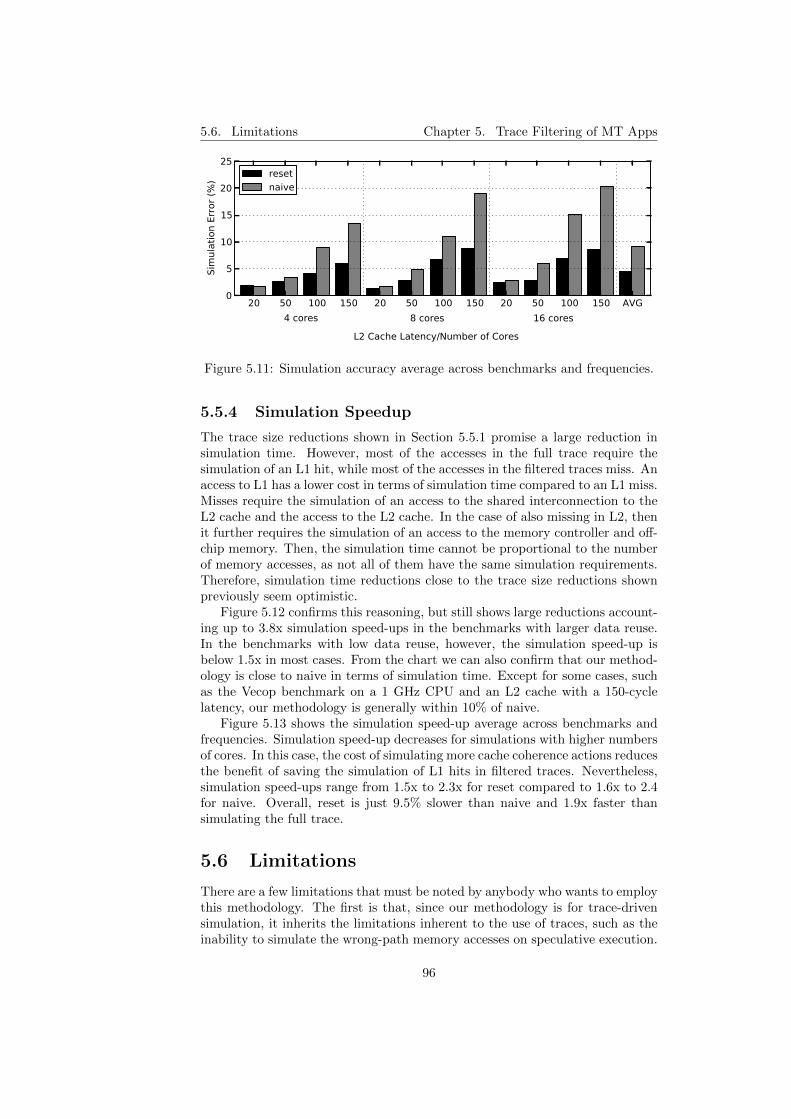
5.6. Limitations Chapter 5. Trace Filtering of MT Apps
20 50 100 150 20 50 100 150 20 50 100 150 AVG0
5
10
15
20
25
Sim
ulat
ion
Erro
r (%
)
4 cores 8 cores 16 cores
resetnaive
L2 Cache Latency/Number of Cores
Figure 5.11: Simulation accuracy average across benchmarks and frequencies.
5.5.4 Simulation Speedup
The trace size reductions shown in Section 5.5.1 promise a large reduction insimulation time. However, most of the accesses in the full trace require thesimulation of an L1 hit, while most of the accesses in the filtered traces miss. Anaccess to L1 has a lower cost in terms of simulation time compared to an L1 miss.Misses require the simulation of an access to the shared interconnection to theL2 cache and the access to the L2 cache. In the case of also missing in L2, thenit further requires the simulation of an access to the memory controller and off-chip memory. Then, the simulation time cannot be proportional to the numberof memory accesses, as not all of them have the same simulation requirements.Therefore, simulation time reductions close to the trace size reductions shownpreviously seem optimistic.
Figure 5.12 confirms this reasoning, but still shows large reductions account-ing up to 3.8x simulation speed-ups in the benchmarks with larger data reuse.In the benchmarks with low data reuse, however, the simulation speed-up isbelow 1.5x in most cases. From the chart we can also confirm that our method-ology is close to naive in terms of simulation time. Except for some cases, suchas the Vecop benchmark on a 1 GHz CPU and an L2 cache with a 150-cyclelatency, our methodology is generally within 10% of naive.
Figure 5.13 shows the simulation speed-up average across benchmarks andfrequencies. Simulation speed-up decreases for simulations with higher numbersof cores. In this case, the cost of simulating more cache coherence actions reducesthe benefit of saving the simulation of L1 hits in filtered traces. Nevertheless,simulation speed-ups range from 1.5x to 2.3x for reset compared to 1.6x to 2.4for naive. Overall, reset is just 9.5% slower than naive and 1.9x faster thansimulating the full trace.
5.6 Limitations
There are a few limitations that must be noted by anybody who wants to employthis methodology. The first is that, since our methodology is for trace-drivensimulation, it inherits the limitations inherent to the use of traces, such as theinability to simulate the wrong-path memory accesses on speculative execution.
96
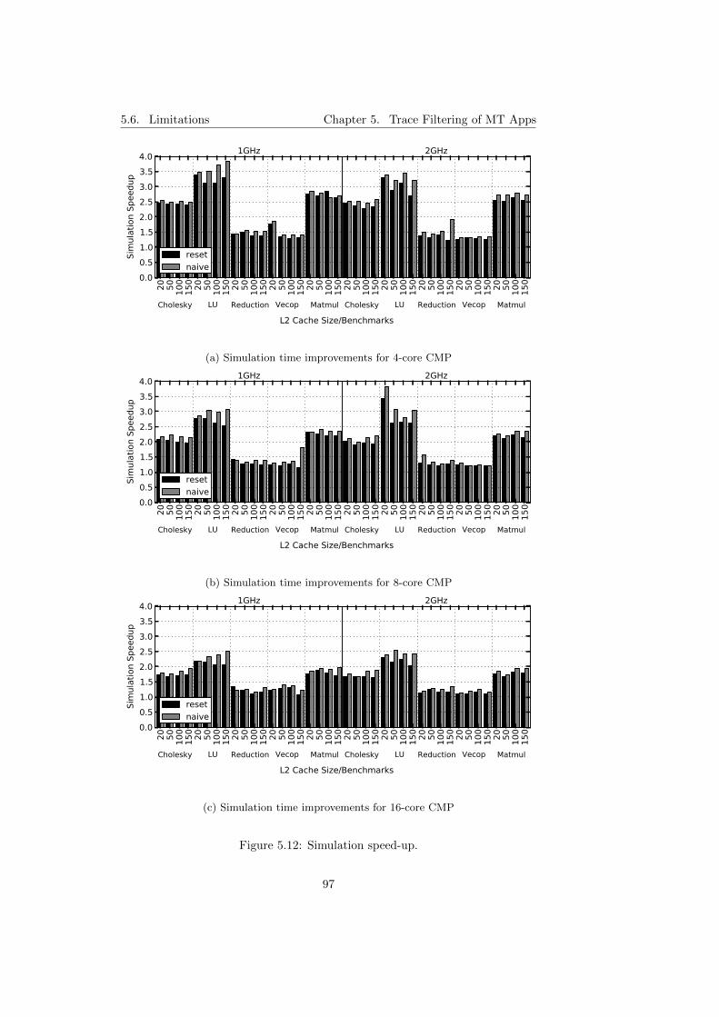
5.6. Limitations Chapter 5. Trace Filtering of MT Apps
20 50 100
150 20 50 100
150 20 50 100
150 20 50 100
150 20 50 100
150 20 50 100
150 20 50 100
150 20 50 100
150 20 50 100
150 20 50 100
1500.0
0.51.01.52.02.53.03.54.0
Sim
ulat
ion
Spee
dup
Cholesky LU Reduction Vecop Matmul Cholesky LU Reduction Vecop Matmul
resetnaive
1GHz 2GHz
L2 Cache Size/Benchmarks
(a) Simulation time improvements for 4-core CMP
20 50 100
150 20 50 100
150 20 50 100
150 20 50 100
150 20 50 100
150 20 50 100
150 20 50 100
150 20 50 100
150 20 50 100
150 20 50 100
1500.0
0.51.01.52.02.53.03.54.0
Sim
ulat
ion
Spee
dup
Cholesky LU Reduction Vecop Matmul Cholesky LU Reduction Vecop Matmul
resetnaive
1GHz 2GHz
L2 Cache Size/Benchmarks
(b) Simulation time improvements for 8-core CMP
20 50 100
150 20 50 100
150 20 50 100
150 20 50 100
150 20 50 100
150 20 50 100
150 20 50 100
150 20 50 100
150 20 50 100
150 20 50 100
1500.0
0.51.01.52.02.53.03.54.0
Sim
ulat
ion
Spee
dup
Cholesky LU Reduction Vecop Matmul Cholesky LU Reduction Vecop Matmul
resetnaive
1GHz 2GHz
L2 Cache Size/Benchmarks
(c) Simulation time improvements for 16-core CMP
Figure 5.12: Simulation speed-up.
97
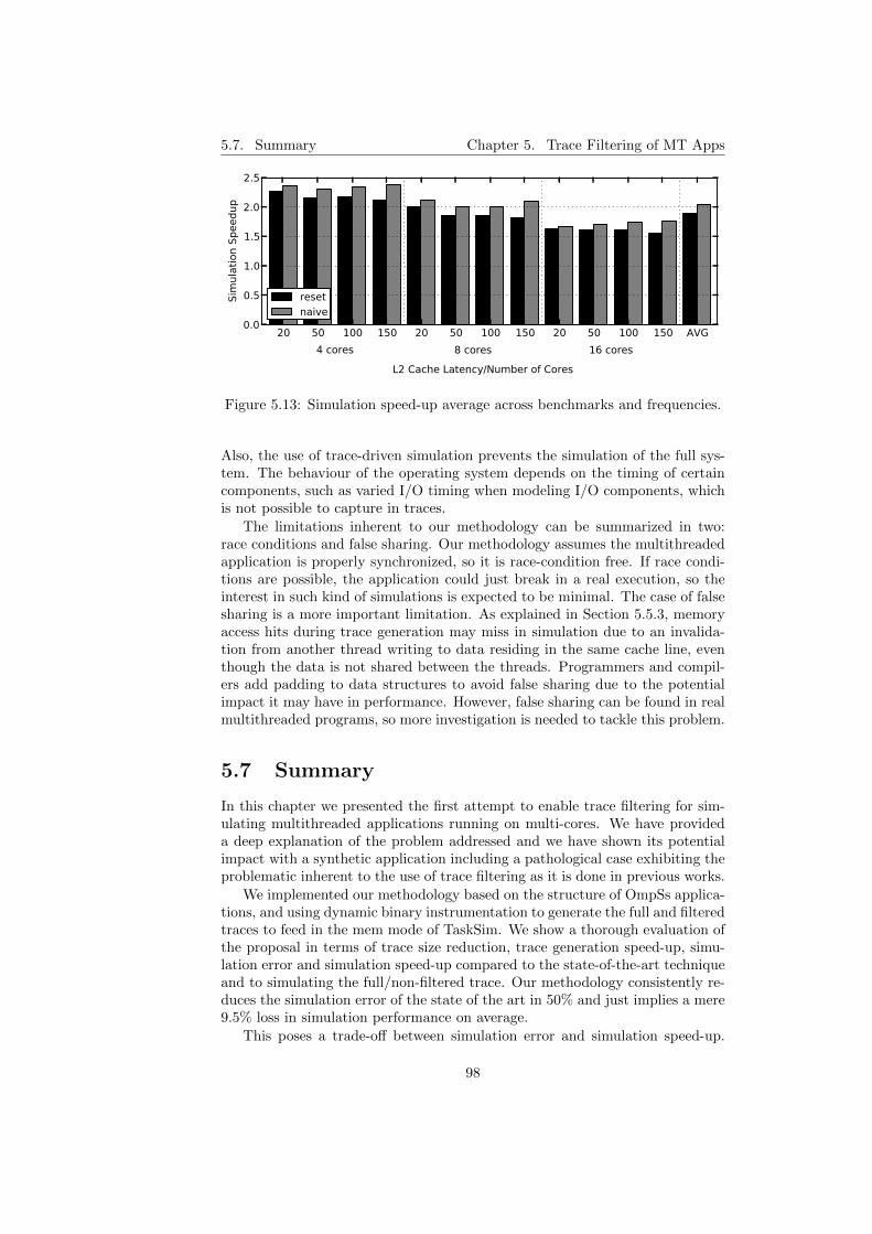
5.7. Summary Chapter 5. Trace Filtering of MT Apps
20 50 100 150 20 50 100 150 20 50 100 150 AVG0.0
0.5
1.0
1.5
2.0
2.5
Sim
ulat
ion
Spee
dup
4 cores 8 cores 16 cores
resetnaive
L2 Cache Latency/Number of Cores
Figure 5.13: Simulation speed-up average across benchmarks and frequencies.
Also, the use of trace-driven simulation prevents the simulation of the full sys-tem. The behaviour of the operating system depends on the timing of certaincomponents, such as varied I/O timing when modeling I/O components, whichis not possible to capture in traces.
The limitations inherent to our methodology can be summarized in two:race conditions and false sharing. Our methodology assumes the multithreadedapplication is properly synchronized, so it is race-condition free. If race condi-tions are possible, the application could just break in a real execution, so theinterest in such kind of simulations is expected to be minimal. The case of falsesharing is a more important limitation. As explained in Section 5.5.3, memoryaccess hits during trace generation may miss in simulation due to an invalida-tion from another thread writing to data residing in the same cache line, eventhough the data is not shared between the threads. Programmers and compil-ers add padding to data structures to avoid false sharing due to the potentialimpact it may have in performance. However, false sharing can be found in realmultithreaded programs, so more investigation is needed to tackle this problem.
5.7 Summary
In this chapter we presented the first attempt to enable trace filtering for sim-ulating multithreaded applications running on multi-cores. We have provideda deep explanation of the problem addressed and we have shown its potentialimpact with a synthetic application including a pathological case exhibiting theproblematic inherent to the use of trace filtering as it is done in previous works.
We implemented our methodology based on the structure of OmpSs applica-tions, and using dynamic binary instrumentation to generate the full and filteredtraces to feed in the mem mode of TaskSim. We show a thorough evaluation ofthe proposal in terms of trace size reduction, trace generation speed-up, simu-lation error and simulation speed-up compared to the state-of-the-art techniqueand to simulating the full/non-filtered trace. Our methodology consistently re-duces the simulation error of the state of the art in 50% and just implies a mere9.5% loss in simulation performance on average.
This poses a trade-off between simulation error and simulation speed-up.
98

5.7. Summary Chapter 5. Trace Filtering of MT Apps
The average error of our technique is 4.5% in our experiments and simulationtime is reduced by half. Research works evaluating small differences in perfor-mance may prefer to reduce the error margin and simulate the full trace even if ittakes twice the time. On the other hand, works requiring very long simulations(several days or weeks) may want to benefit from a 2x cutdown in simulationtime at the expense of a relatively small simulation error.
99

5.7. Summary Chapter 5. Trace Filtering of MT Apps
100

Chapter 6
Modeling the RuntimeSystem Timing
The methodology presented in Chapter 3 simulates sequential sections usingtraces and executes parops directly on the host machine at simulation time.Using native execution is fast but difficults the timing modeling of parop ex-ecution on the simulated machine because parop execution is not exposed thesimulation engine.
Runtime-managed applications are usually partitioned keeping in mind theoverhead of parop execution so the time spent on parops is negligible comparedto the time spent in sequential sections between them. However, in applicationsusing fine-grained parallelism to scale to large numbers of cores, parop executionmay have a significant performance impact.
In this chapter, we evaluate the importance of modeling the timing of paropsand present our attempt to use a fast high-level model for parop timing basedon their execution on the host machine.
6.1 Problem
Figure 6.1 shows the timeline of a simulation using our methodology in Chap-ter 3. The simulated application is task-based, runs on a configuration with twosimulated threads and uses a master-worker scheme where one thread createstasks and another one executes them. Figure 6.1(a) shows the application tracefile content and the corresponding simulation stages on the multiple simula-tion components, namely the two simulated threads and the integrated runtimesystem. The trace file includes sequential sections, shown as CPU events, andparop call events. Simulation starts in Thread 0 and, after a first sequential sec-tion (A), simulation finds a create task event. Then, the simulation enginecalls the runtime system through the Runtime Bridge (see Figure 3.4) to createTask 1. This operation is executed by the runtime system, which takes somehost time and, having finished, simulation resumes. Then, Thread 1, which wasidle waiting for tasks (dashed line), asks the runtime system for a ready task,and it is assigned the recently-created Task 1. Thread 1 starts simulating Task 1(which has its separate trace not shown in the figure).
Simulation proceeds analogously in Thread 0 with the creation of Task 2,
101

6.1. Problem Chapter 6. Modeling the Runtime System Timing
Simulated
Thread 0
Trace File
CPU A
create_task 1
Runtime
System
CPU B
create_task 2
Simulated
Thread 1
...
...
...
CPU C ...
task_wait
host time
CPU E
...
Thread 0 Thread 1...
sim
ula
tor
tim
e
a) Simulation Operation b) Simulated Timing
seq. sections parop calls parop exec. idle
A B B C D E
F F
A
B
C
D
E
F
Figure 6.1: Simulation example of a task-based application running on twothreads. (a) The simulation alternates between the simulated threads and theruntime system operation, to simulate the actions specified in the events in-cluded in the trace. The runtime system performs the creation of tasks, andassign tasks to idle threads (dashed line), such as Task 1 to Thread 1. (b) Thesimulation engine does not account the timing of the runtime system operations,and only simulates the timing of the sequential sections in the trace.
and so on. Later, close to the end of the application, a task wait event is found,which forces Thread 0 to wait for all previously-created tasks to complete. Thesimulation engine calls the runtime system for this synchronization primitiveand, when executed, it founds that all tasks have finished. Simulation resumesand completes after simulating the last sequential section.
At simulation time, the simulator alternates between timing simulation in thetrace-driven simulation engine and parop execution in the runtime system. Theproblem is that the trace-driven simulator is not aware of the executed runtimesystem operations, and it can only model the timing of sequential sections inthe trace, as it is shown in Figure 6.1(b). This way, the simulator is able toreflect the impact of the runtime system decisions on the application execution,such as tasks being scheduled to different threads. However, it does not accountfor the overhead of the runtime system operations themselves.
A straightforward approach to account for parop timing is to use the timetaken by the operation during trace generation as an estimate for its executiontime. The problem with this technique is that the trace generation run uses aspecific runtime configuration, including options such as scheduling and cutoffpolicies (see Section 2.7). Therefore, the problem with this technique is that thetiming of parops would be the same (the one at trace generation time) regardlessof the runtime system configuration used during simulation.
The work presented in this chapter has therefore two objectives. First, eval-uate the variability of parop timing for different runtime system and simulatedmachine configurations. And second, to model the timing of parops so simula-tion reflects the performance impact of different runtime system configurationsin the predicted execution time on the simulated machine.
102

6.2. Runtime Analysis Chapter 6. Modeling the Runtime System Timing
6.2 Runtime Analysis
Generally, runtime system operations take a small portion of the total applica-tion time: applications are appropriately partitioned, and runtime systems arehighly optimized, both to minimize runtime system overheads. However, not allapplications can be easily repartitioned, as the problem size for a determinedcomputation slice may be fixed, for example, the size of a macroblock in videodecoding applications. Also, advanced runtime system policies, such as locality-aware schedulers, may provide a better application performance, but their costlyoperation may cancel out their benefits, even leading to performance degrada-tion in some scenarios. In other words, the overhead of a better scheduler maycancel out the benefits of its better scheduling.
In order to understand the factors affecting the performance of runtimesystem operations, we analyze their computation on different scenarios and thepossible situations of contention on shared resources. The object of this studyis the NANOS++ runtime system, which is the one used along this thesis. Also,we focus on the parops used in task-based parallel applications written in theOmpSs programming model (see Section 2.7.1).
One of the factors introducing performance variability in NANOS++ paropsis the use of cut-off mechanisms (see Section 2.7), referred to as throttling.Whenever the application wants to create a new task, the throttling mecha-nism decides whether to actually spawn the new task and add it to the taskdependence graph, so any thread can execute it, or tell the thread creating thetask to execute it inline. This mechanism aims to alleviate the cost of addingmore tasks to the runtime system structures when there is no need for moreparallelism, such as when all treads are busy and there are many pending tasks.
Examples of throttling metrics are the total number of in-flight tasks and thetotal number of ready tasks at a given point in time. When the metric is abovea certain threshold, referred to as throttle-limit, additional tasks are executedinline rather than created and submitted for execution by other threads.
Another important factor introducing parop variability is the scheduler. Itmakes decisions regarding task queuing and execution at certain points of theapplication, such as on task creation, task completion and when a thread be-comes idle. For this, it manages ready task queues. A ready task queue includesa set of tasks ready for execution (dependencies satisfied), and may be global orthread-private. Different schedulers may have different policies, such as breadth-first and work-first [70], and therefore have different algorithm complexities.
Figure 6.2 shows the pseudo-code of four of the main runtime system op-erations in NANOS++. For each of these operations, we indicate whether itaccesses or updates the task dependence graph (DG) or the ready task queues(RQ). Figure 6.2a shows the code for task creation. As previously mentioned,due to the throttling mechanism, the execution may follow different paths withpotentially different costs. Also, if a task is actually submitted (no throttle), anddoes not have any potential dependencies, it is considered independent, and isdirectly pushed to a ready task queue. However, if it has potential dependen-cies, it must be checked against previous tasks in the task dependence graphand, if there are dependencies, the graph is updated accordingly with the newtask.
Another example of variability is the acknowledge of task completion, shownin Figure 6.2b. The operation after completing a task must iterate over its
103
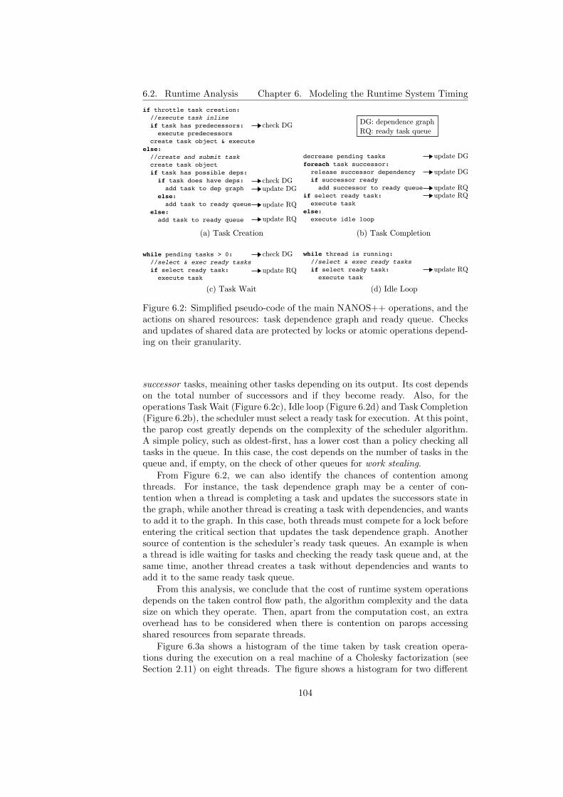
6.2. Runtime Analysis Chapter 6. Modeling the Runtime System Timing
if throttle task creation: //execute task inline if task has predecessors: execute predecessors create task object & executeelse: //create and submit task create task object if task has possible deps: if task does have deps: add task to dep graph else: add task to ready queue else: add task to ready queue
check DG
check DGupdate DG
update RQ
update RQ
(a) Task Creation
check DGwhile pending tasks > 0: //select & exec ready tasks if select ready task: execute task
update RQ
(c) Task Wait
while thread is running: //select & exec ready tasks if select ready task: execute task
update RQ
(d) Idle Loop
DG: dependence graph
RQ: ready task queue
decrease pending tasksforeach task successor: release successor dependency if successor ready add successor to ready queueif select ready task: execute taskelse: execute idle loop
update RQ
(b) Task Completion
update DG
update DG
update RQ
Figure 6.2: Simplified pseudo-code of the main NANOS++ operations, and theactions on shared resources: task dependence graph and ready queue. Checksand updates of shared data are protected by locks or atomic operations depend-ing on their granularity.
successor tasks, meaining other tasks depending on its output. Its cost dependson the total number of successors and if they become ready. Also, for theoperations Task Wait (Figure 6.2c), Idle loop (Figure 6.2d) and Task Completion(Figure 6.2b), the scheduler must select a ready task for execution. At this point,the parop cost greatly depends on the complexity of the scheduler algorithm.A simple policy, such as oldest-first, has a lower cost than a policy checking alltasks in the queue. In this case, the cost depends on the number of tasks in thequeue and, if empty, on the check of other queues for work stealing.
From Figure 6.2, we can also identify the chances of contention amongthreads. For instance, the task dependence graph may be a center of con-tention when a thread is completing a task and updates the successors state inthe graph, while another thread is creating a task with dependencies, and wantsto add it to the graph. In this case, both threads must compete for a lock beforeentering the critical section that updates the task dependence graph. Anothersource of contention is the scheduler’s ready task queues. An example is whena thread is idle waiting for tasks and checking the ready task queue and, at thesame time, another thread creates a task without dependencies and wants toadd it to the same ready task queue.
From this analysis, we conclude that the cost of runtime system operationsdepends on the taken control flow path, the algorithm complexity and the datasize on which they operate. Then, apart from the computation cost, an extraoverhead has to be considered when there is contention on parops accessingshared resources from separate threads.
Figure 6.3a shows a histogram of the time taken by task creation opera-tions during the execution on a real machine of a Cholesky factorization (seeSection 2.11) on eight threads. The figure shows a histogram for two different
104

6.3. Runtime Modeling Chapter 6. Modeling the Runtime System Timing
0 10 20 30Time (us)
02000400060008000
10000120001400016000
Task
Cre
atio
n Co
unt
throttle-limit=5throttle-limit=500
(a) Task Creation Time Distribution
5 100 500 10000Throttle Limit (4/8/16 threads)
012345678
Lock
Wai
t Tim
e (m
s)
SwitchingTaskGraphScheduler
(b) Average Lock Wait Time per Thread
Figure 6.3: Runtime system operation variability. (a) Task creation cost distri-bution of Cholesky factorization run on eight threads for two different throttlinglimits. (b) Breakdown of the lock contention time of Cholesky decompositionrun on four, eight and sixteen threads for four different throttling limits.
throttling limits, 5 and 500. Whenever the total number of in-flight tasks isabove the limit, new tasks are executed inline instead of following the regularsubmission to the task graph or ready queues. Hence, a lower throttle limitgenerates more inlining than a higher one. The results in the figure show thatusing a throttle limit of 5 leads to lower task creation costs than using a limit of500, as many more tasks are inlined. Most of the inlined creations take less than10 us, while the regular creation and submission takes between 5 and 20 us.
Figure 6.3b shows the average time per thread spent waiting for acquiring alock, and its breakdown depending on the operation being synchronized. This isshown for Cholesky factorization using multiple numbers of throttle limits andrun on four, eight and sixteen threads. The results show two effects. The firstis that lock contention increases with the number of threads for all throttlinglimits. This is because there are more chances that separate threads want toaccess a shared resource when there are more threads executing in parallel. Thesecond is that the contention on locks also increases after a certain throttle limit.The contention for locks with limit 5 is significantly lower than for larger limits.This is because in inlined task creations the runtime system does not need toaccess shared resources.
6.3 Runtime Modeling
The results in the previous section show that the cost of parops is sensible tothe runtime system and simulated machine configurations, and how these affectthe contention on the runtime system shared resources. Therefore, in situationswhere parops account for a large portion of the application, or when multipleruntime system configurations are compared in terms of overhead, it is necessaryto account for time spent in parop execution.
In this section, we introduce a fast high-level timing model for parops, to beused in the simulation methodology in Chapter 3. The objective is to providean estimate of parop execution time, while maintaining the cost of the model
105

6.3. Runtime Modeling Chapter 6. Modeling the Runtime System Timing
Thread 0 Thread 1
get start time
get stop timesimulateruntimeperiod continue
processingtrace
Runtime Thread 0
getlock/unlocktime
waitingtime
simulatelocks
Runtime
seq. section parop exec.parop call sim. parop sim. lock wait
Figure 6.4: Simulation example with host time only (left) and host time plussimulation of locks (right).
low, so it is fast enough to be used in multiple levels of abstraction from detailedto high-level ones.
The timing model lies on top of a light-weight instrumentation library thatcaptures the execution time of parops in the host machine. This gives a measureof the cost of that operation considering the runtime system state during simula-tion. As the runtime system data state depends on the simulated architecture,the control flow path followed by parop execution, the algorithm complexityand the data size on which it operates are reflected by the parop executiontime on the host. Then, the host execution time can be factored to match thesimulated machine performance. The use of performance factors has alreadybeen explored in existing simulation tools [24, 155], and several databases ofperformance factors are publicly available [9, 158].
From the previous section we know that, apart from parop computation,contention on shared resources also depends on the runtime system configura-tion. On a sequential simulator, the simulation of different threads is serializedand, thus, the execution of parops on different simulated threads is also seri-alized. Therefore, all lock acquire operations are successful and the potentialcontention is not reproduced. To account for contention, the lock acquire andrelease operations are also instrumented. As a result, when the control comesback to the simulation engine after a parop execution, the simulator has a traceof sequential sections and lock operations of the executed parop that is used tomodel its timing.
Figure 6.4 illustrates how the parop execution information is captured andused for simulation. The figure shows the methodology’s operation for a paropexecution without (left) and with (right) locks. Without locks, on a paropexecution, its starting and finishing times are recorded, and its total executiontime is computed. The resulting trace is a single sequential section with a givenexecution time (on which a performance factor can be applied to match thesimulated machine performance). Finally, the resulting sequential section timeis accounted in the parop-calling simulated thread, that resumes processing thetrace afterwards.
106
6.4. Evaluation Chapter 6. Modeling the Runtime System Timing
The example with locks shows how lock acquire and release operations, thatdo not suffer from contention during the execution on the host machine, arealso included in the resulting trace. In Figure 6.4 (right), both threads executeparops that are serialized. However, when they simulate both parop traces,Thread 0 acquires the lock first, and then Thread 1 fails to acquire the samelock and has to wait before Thread 0 releases it, thus reproducing the contentionthat would exist on that application running on the simulated machine.
6.4 Evaluation
In this section we present a set of experiments to show the impact of throttlinglimits, scheduling policies and numbers of threads on parop execution and howour methodology models their timing.
We use the integrated TaskSim-NANOS++ simulation infrastructure pre-sented in Chapter 3 and simulate with the burst mode presented in Chapter 4.The experiments compare the following configurations:
• Real: execution on the real machine.
• Naive: simulation using as parop execution time the one from the tracegeneration run (explained in Section 6.1).
• Host: simulation using as parop execution time the one from the hostmachine during simulation (Figure 6.4 (left)).
• Host+Locks: simulation using as parop execution time the one from thehost maching during simulation and also simulating lock contention fromparops in different simulated threads (Figure 6.4 (right)).
For the first experiment we use a blocked-matrix multiplication with 64×64blocks of single-precision floating-point elements written in OmpSs. We executethe application in the real machine and using the three aforementioned simu-lation configurations. All experiments are done with two different schedulers:default and cilk. Default uses a global ready queue and a LIFO policy. Cilkuses one queue per thread and, on task creation, it starts executing the createdtask and the parop-calling task gets enqueued for other thread to resume itsexecution. Executions on the real machine are repeated five times and averagedto counteract OS noise.
Figure 6.5 shows the normalized execution time on the real machine and onsimulation using the naive, host and host+locks approaches. The x-axis showsthrottling limit values from 1 to 9999999 (infinite) and each data series is fora given number of threads. The results are normalized to the execution withthrottling limit 1.
The naive configuration is able to reproduce the lack of parallelism of throt-tling limits below 50, but is not able to reproduce the loss of performance forlarger throttling limits due to parop overhead. The introduction of the hosttime in the host configuration is able to account for part of that overhead butdoes not make as much difference as in the real machine. The simulation oflocks gets the predicted execution time closer to the one of the real machine butit does not follow the same trends and does not match its magnitude either.
107

6.4. Evaluation Chapter 6. Modeling the Runtime System Timing
0.90
0.95
1.00
1.05No
rmal
ize
Exec
utio
n Ti
me
(a) real
1 threads2 threads4 threads8 threads12 threads16 threads
(b) naive
1 5 10 50 100
500
1000
1000
0
9999
999
Throttle Limit
0.90
0.95
1.00
1.05
Norm
aliz
e Ex
ecut
ion
Tim
e
(c) host
1 5 10 50 100
500
1000
1000
0
9999
999
Throttle Limit
(d) host+locks
Figure 6.5: Normalized execution time real (a) and simulated (b,c,d) for ablocked-matrix multiplication using 64×64 blocks.
In any case, parop execution time in these experiments is not significant,and the results are in the noise margin which can be affected by the inherentinaccuracies of the burst mode and OS noise during the real, trace generationand simulation executions.
To get a more precise view of the effects of our methodology, we carry outa second case study using an H.264 decoder skeleton application written inOmpSs. This skeleton has the same structure as a real implementation of anH.264 decoder using the 3D wave optimization [117]. In this case, we focus onthe parop timing across multiple schedulers and numbers of threads and use athrottling limit of 100 for all experiments.
The experiments are done for a set of schedulers including the ones in the
108

6.5. Discussion Chapter 6. Modeling the Runtime System Timing
NANOS++ distribution (default, bf, dbf, cilk, wf) and two other schedulersusing priorities depending on the chain of dependencies a given task has tothe top of the task dependence graph (toplev) and to the bottom of the graph(botlevel). These schedulers are explained in more detailed in the PhD Thesis ofPaul Carpenter [54]. The complexity of toplev and botlev is higher than for theother five scheduler, because they have to traverse the task dependence graphto assign priorities to tasks.
defau
lt bf dbf
cilk wftop
levbo
tlev
Schedulers
0
2
4
6
8
10
12
14
Tim
e (s
econ
s)
realhost
(a) Four threads
defau
lt bf dbf
cilk wftop
levbo
tlev
Schedulers
0
2
4
6
8
10
12
14Ti
me
(sec
ons)
realhost
(b) Eight threads
defau
lt bf dbf
cilk wftop
levbo
tlev
Schedulers
0
2
4
6
8
10
12
14
Tim
e (s
econ
s)
realhost
(c) Sixteen threads
Figure 6.6: Task creation execution time of the H.264 decoder skeleton both inthe real machine and using the host simulation approach using multiple numbersof threads.
Figure 6.6 shows the task creation execution time for the real machine (a)and using the host simulation approach (b) for the aforementioned schedulersand multiple numbers of threads. In the real machine, the differences for thefive schedulers in the NANOS++ distribution are not significant and can beconsidered noisy. However, the cost of toplev and botlev is very significant.However, the host simulation approach is not able to reproduce that cost. Wehave checked the source of the overhead for these scheduler in the real machine,and it comes from the increased complexity of the task graph insertion ratherthan from the contention in locks, which is minimal. Therefore, the simulationof locks is not expected to improve this prediction.
6.5 Discussion
The experiments in the previous section show that our high-level model is notable to accurately reproduce the variability of different runtime system config-urations at simulation time. The fundamental deficiencies of the method arerelated to caching effects due to the following facts:
• Serial vs. parallel execution. The simulator runs on a single host threadwhile the real application executes on multiple separate threads. This hastwo effects. The first is that parops executing in different threads will
109

6.6. Summary Chapter 6. Modeling the Runtime System Timing
have different cache states in their privates caches while the simulator hasa single private cache in which the state of the runtime system can be kept.The second is that the cache coherence actions that happen in the realmachine from accesses to shared runtime system resources from separatethreads are not present during simulation either.
• Application data vs. simulator data. In the real machine, between twoparop calls, the application computation may have completely evicted allruntime system data from the caches. In the simulator, this depends onthe level of abstraction of the timing model of sequential sections betweenparop calls. In a high-level mode such as the burst mode, the computationbetween parop calls is small and the runtime system data may be kept inthe private caches and the accesses in the next parop call will hit in thecache.
These two deficiencies lead to the underestimations of parop execution forsome schedulers seen in the previous section.
Another deficiency of the method is instrumentation overheads. The exe-cution of some parops is short and the insertion of instrumentation points canlead to overestimations when simulating the timing of parops using the hostand host+locks approaches, as we have seen for some schedulers. A possiblesolution to this problem is to measure the typical delay of an instrumentationcall and subtract it from the measured parop execution time.
As a result, the parop timing models introduced in this chapter are notenough for an accurate reproduction of the time taken by runtime system op-erations. Further investigation is needed to quantify the deficiencies analyzedin this discussion and propose more detailed models that actually account forthe runtime system effects when the cost of the runtime system operations is ofinterest of the research study being carried out.
6.6 Summary
In this chapter we explained the problem of modeling the timing of the runtimesystem operations using our simulation methodology in Chapter 3. We showedthe sources of variability for runtime system operations and proposed two high-level models for the timing of these operations based on their execution on thehost machine.
Our experiments showed that our models are able to partially mimic thetrends of parop timing and are definitely better than the naive approach, butgenerally result in underestimations. We discussed the reasons for these in-accuracies and concluded that further investigation is needed to quantify thedeficiencies of these methods and improve the models to bridge the gap betweenthe simulated and real parop execution times.
110

Chapter 7
Conclusions
In the history of microprocessor from 1972, the number of transistors per chiphas doubled every two years. Due to power density issues, among others, thisincreasing number of chips has been used since the early 2000s to include morecores in the same chip.
The inclusion of multiple cores per chip, has changed the microprocessordesign paradigm, which has an impact on single-thread performance. The de-sign of multi-cores focuses on exploiting thread-level parallelism on multiplecores, rather than instruction-level parallelism on a single core. This leads to aslowdown on the increase of single-thread performance that went from doublingevery two years until 2004, to doubling every three years and a half since then.
These two facts, the increasing trends of number of transistors per chip andsingle-thread performance, has an impact on computer architecture simulation,which is the topic in this thesis. Computer architecture simulation is importantbecause it drives most computer architecture research. In this context, thenumber of transistors determines the complexity of the model to be simulated,and the single-thread performance of the host machine determines simulationspeed. Since the number of transistors keeps doubling every two years, thecomplexity of the simulated model also increases at this rate. At the same time,single-thread performance, and thus, simulation speed, doubles every three yearsand a half. The difference is what we call the simulation speed gap, and makessimulation of multi-cores increasingly slow over time. As an example, if thesimulation of a contemporary architecture takes one week, a simulation of acontemporary architecture in five years will take more than two weeks, and overa month in ten years.
The objective of this thesis is to close the simulation speed gap to reducesimulation time. Other researchers in the computer architecture community areaware of the problem and have proposed techniques to reduce simulation time,such as sampling and parallelization, that we covered in Section 2.4.
The approach in this thesis is to raise the level of abstraction to close thesimulation speed gap and reduce simulation time. In this direction, we haveproposed a set of simulation techniques and methodologies. In the next sections,we summarize our contributions and list their associated publications, explainworks that have used our research, and provide some recommendations on howthis work could be continued in the future.
111

7.1. Contributions and Publications Chapter 7. Conclusions
7.1 Contributions and Publications
Our contributions in this thesis are the following:
• A trace-driven simulation methodology for dynamically-scheduledmultithreaded applications. It combines a trace-driven simulation enginewith a runtime system to simulate timing-independent user code usingtraces and execute timing-dependent parops at simulation time to makescheduling and synchronization decisions based on the simulated machine.
[150] A. Rico, A. Duran, F. Cabarcas, Y. Etsion, A. Ramirez, M. Valero.Trace-driven Simulation of Multithreaded Applications. In Proceed-ings of the IEEE International Symposium on Performance Analysisof Systems and Software, ISPASS ’11, pages 87–96, Apr. 2011.
[151] A. Rico, A. Duran, A. Ramirez, M. Valero. Simulating Dynamically-Scheduled Multithreaded Applications Using Traces. IEEE Micro.Submitted for publication.
• Two fast high-level simulation modes for evaluating application scal-ability and accelerators with scratchpad memories. These simulation modesare based on our definition of application abstraction. At the highest levelof abstraction, the burst mode, is faster than native execution and is ac-curate and useful to predict application scalability on larger numbers ofcores than the ones available in the real machine. The inout mode hasonly an average 25x slowdown compared to native execution, and has beenshown accurate and useful for the simulation of accelerator-based architec-tures. The most important fact is that these modes have been shown to befaster and more insightful than functional simulation in execution-drivensimulators.
[148] A. Rico, F. Cabarcas, C. Villavieja, M. Pavlovic, A. Vega, Y. Etsion,A. Ramirez, M. Valero. On the Simulation of Large-Scale Architec-tures Using Multiple Application Abstraction Levels. ACM Trans.Archit. Code Optim., 8(4):36:1–36:20, 2012.
• A trace generation technique to include memory accesses sensible tocache invalidations in filtered memory access traces for the simulationof multithreaded applications running on cache-based multi-cores. Thetrace generation technique covers invalidations due to different thread in-terleavings and different dynamic scheduling decisions. It reduces theaverage error of the state of the art from 9% to 4.5%, while providingsimilar trace size reduction (10x smaller traces) and simulation speed-up(2x faster simulations) compared to the simulation of the full trace.
[154] A. Rico, A. Ramirez, M. Valero. Trace Filtering of MultithreadedApplications for CMP Memory Simulation. In Proceedings of theIEEE International Symposium on Performance Analysis of Systemsand Software, ISPASS ’13, pages 134–135, Apr. 2013.
• A high-level simulation model for modeling the timing of executedparops in our simulation methodology. We found that our technique isnot enough to faithfully model the timing of parops due to the different
112
7.2. Impact Chapter 7. Conclusions
application and cache states between simulation and real execution. Fur-ther investigation is needed to improve the model to better account forparop timing in the applications or studies where it is relevant.
7.2 Impact
In this section we explain other works we carried out related with the work inthis thesis; works that use the simulation techniques proposed in this thesis; andother non-related works we have carried out during the course of this thesis.
7.2.1 Our Related Work
Related to the development of CellSim, we published a set of papers, posterabstracts, and a workshop presentation. In chronological order:
[49] F. Cabarcas, A. Rico, D. Rodenas, X. Martorell, A. Ramirez, E. Ayguade.A module-based cell processor simulator. In Advanced Advanced Com-puter Architecture and Compilation for High-Performance and EmbeddedSystems 2006 Poster Abstracts, ACACES ’06, pages 237–240, July 2006.
[50] F. Cabarcas, A. Rico, D. Rodenas, X. Martorell, A. Ramirez, E. Ayguade.CellSim: A Cell Processor Simulation Infrastructure. In Advanced Com-puter Architecture and Compilation for Embedded Systems 2007 PosterAbstracts, ACACES ’07, pages 279–282, July 2007.
[147] A. Rico, F. Cabarcas, D. Rodenas, X. Martorell, A. Ramirez, E. Ayguade.Implementation and validation of a Cell simulator (Cellsim) using UNISIM.In 3rd HiPEAC Industrial Workshop on Compilers and Architectures, Apr.2007.
[51] F. Cabarcas, A. Rico, D. Rodenas, X. Martorell, A. Ramirez, E. Ayguade.CellSim: A Validated Modular Heterogeneous Multiprocessor Simulator.In XVIII Jornadas de Paralelismo (CEDI 2007: II Congreso Espanol deInformatica), JP ’07, pages 187–188, Sept. 2007.
Related to CellSim, we also carried out a full-day Tutorial at the SixteenthInternational Conference on Parallel Architectures and Compilation Techniques(PACT) 2007:
[142] A. Ramirez, A. Rico, F. Cabarcas. CellSim: a Modular Simulator for Het-erogeneous Chip Multiprocessors. http://pcsostres.ac.upc.edu/cellsim/doku.php#cellsim_tutorial_documentation, 15 Sept.2007. Full-day tutorial at Parallel Architectures and Compilation Tech-niques (PACT) 2007.
Related to the development of TaskSim, we published a technical report atthe Universitat Politecnica de Catalunya – BarcelonaTech:
[146] A. Rico, F. Cabarcas, A. Quesada, M. Pavlovic, A. J. Vega, C. Villavieja,Y. Etsion, and A. Ramirez. Scalable Simulation of Decoupled Accelera-tor Architectures. Technical Report UPC-DAC-RR-2010-14, UniversitatPolitecnica de Catalunya, June 2010.
113

7.2. Impact Chapter 7. Conclusions
Related to the analysis of the runtime system overheads, we published ajournal and a conference paper related to the task creation bottleneck mentionedat several points along the thesis and explained in Section 3.5. In chronologicalorder:
[152] A. Rico, A. Ramirez, M. Valero. Task Management Analysis on the CellBE. In XIX Jornadas de Paralelismo, JP ’08, pages 271–276, Sept. 2008.
[153] A. Rico, A. Ramirez, M. Valero. Available Task-level Parallelism on theCell BE. Scientific Programming, 17(1-2):59–76, 2009.
7.2.2 Other Works using Our Work
During the course of this thesis we developed a set of simulation tools andmethodologies. In this section we give a measure of the impact of our worklisting the publications using our tools and methodologies for the evaluation oftheir proposals.
• List of publications using CellSim in chronological order:
[112] D. Ludovici G. Gaydadjiev. SARC Power Estimation Methodology.In Proceedings of the 18th Annual Workshop on Circuits, Systemsand Signal Processing, Nov. 2007.
[87] R. Giorgi, N. Puzovic, and Z. Popovic. Implementing DTA supportin CellSim. In Advanced Computer Architecture and Compilation forEmbedded Systems 2008 Poster Abstracts, ACACES ’08, July 2008.
[118] C. Meenderinck B. Juurlink. A Chip MultiProcessor Accelerator forVideo Decoding. In Proceedings 19th Annual Workshop on Circuits,Systems and Signal Processing, Nov. 2008.
[84] R. Giorgi, Z. Popovic, N. Puzovic. Exploiting DMA to enable non-blocking execution in Decoupled Threaded Architecture. In IEEEInternational Symposium on Parallel Distributed Processing, IPDPS2009, pages 1–8, 2009.
[85] R. Giorgi, Z. Popovic, N. Puzovic. Implementing Fine/MediumGrained TLP Support in a Many-Core Architecture. In Proceedingsof the 9th International Workshop on Embedded Computer Systems:Architectures, Modeling, and Simulation, SAMOS ’09, pages 78–87,2009.
[86] R. Giorgi, Z. Popovic, N. Puzovic. Introducing Hardware TLP Sup-port in the Cell Processor. In International Conference on Complex,Intelligent and Software Intensive Systems, CISIS ’09, pages 657–662,2009.
[94] X. Huang, X. Fan, S. Zhang, L. Shi. Investigation on Multi-GrainParallelism in Chip Multiprocessor for Multimedia Application. InInternational Conference on Information Engineering and ComputerScience, ICIECS 2009, pages 1–4, 2009.
[78] E. Fernandez Abeledo. Implementation of Nexus: Dynamic Hard-ware Management Support for Multicore Platforms. Master’s thesis,Delft University of Technology, 2010.
114

7.2. Impact Chapter 7. Conclusions
[90] C. Gou, G. Kuzmanov, G. N. Gaydadjiev. SAMS multi-layout mem-ory: providing multiple views of data to boost SIMD performance.In Proceedings of the 24th ACM International Conference on Super-computing, ICS ’10, pages 179–188, 2010.
[41] M. Briejer, C. Meenderinck, B. Juurlink. Extending the Cell SPEwith Energy Efficient Branch Prediction. In Proceedings of the 16thinternational Euro-Par conference on Parallel processing: Part I, Eu-roPar’10, pages 304–315, 2010.
[61] C. Ciobanu, G. Kuzmanov, G. Gaydadjiev, A. Ramirez. A Polymor-phic Register File for Matrix Operations. In International Conferenceon Embedded Computer Systems, SAMOS ’10, pages 241–249, 2010.
[119] C. Meenderinck, B. Juurlink. Nexus: Hardware Support for Task-Based Programming. In 14th Euromicro Conference on Digital Sys-tem Design, DSD ’11, pages 442–445, 2011.
[23] A. Azevedo, B. Juurlink. An Instruction to Accelerate SoftwareCaches. In Proceedings of the 24th international conference on Ar-chitecture of computing systems, ARCS’11, pages 158–170, 2011.
• List of publications using TaskSim in burst mode in chronological order:
[75] Y. Etsion, F. Cabarcas, A. Rico, A. Ramirez, R. M. Badia, E. Ayguade,J. Labarta, M. Valero. Task Superscalar: An Out-of-Order TaskPipeline. In Proceedings of the 2010 43rd Annual IEEE/ACM Inter-national Symposium on Microarchitecture, MICRO ’10, pages 89–100,2010.
• List of publications using TaskSim in inout mode in chronological order:
[48] F. Cabarcas, A. Rico, A. Ramirez, Y. Etsion, C. Villavieja, A. J.Vega, M. Pavlovic, A. Quesada, P. Bellens, R. M. Badia, M. Valero.Castell: A CMP architecture scalable to hundreds of processors.Technical Report UPC-DAC-RR-CAP-2009-33, Universitat Politec-nica de Catalunya, Nov. 2009.
[170] A. Vega, A. Rico, F. Cabarcas, A. Ramirez, M. Valero. Compar-ing Last-level Cache Designs for CMP Architectures. In Proceedingsof the Second International Forum on Next-Generation Multicore/-Manycore Technologies, IFMT ’10, pages 2:1–2:11, 2010.
[47] F. Cabarcas, A. Rico, Y. Etsion, A. Ramirez. Interleaving Granu-larity on High Bandwidth Memory Architecture for CMPs. In Inter-national Conference on Embedded Computer Systems, SAMOS ’10,pages 250–257, 2010.
[141] A. Ramirez, F. Cabarcas, B. Juurlink, A. Mesa, F. Sanchez, A. Azevedo,C. Meenderinck, C. Ciobanu, S. Isaza, G. Gaydadjiev. The SARCArchitecture. Micro, IEEE, 30(5):16–29, 2010.
[62] C. B. Ciobanu, X. Martorell, G. K. Kuzmanov, A. Ramirez, G. N.Gaydadjiev. Scalability Evaluation of A Polymorphic Register File:A CG Case Study. In Proceedings of the 24th International Confer-ence on Architecture of Computing Systems, ARCS’11, pages 13–25,2011.
115
7.2. Impact Chapter 7. Conclusions
[96] S. Isaza, F. Sanchez, F. Cabarcas, A. Ramirez, G. Gaydadjiev. Parametriz-ing Multicore Architectures for Multiple Sequence Alignment. InProceedings of the 8th ACM International Conference on ComputingFrontiers, CF ’11, pages 31:1–31:10, 2011.
[169] A. Vega, F. Cabarcas, A. Ramirez, M. Valero. Breaking the Band-width Wall in Chip Multiprocessors. In International Conference onEmbedded Computer Systems, SAMOS ’11, pages 255–262, 2011.
[16] M. Alvarez, F. Cabarcas, A. Ramırez, C. Meenderinck, B. Juurlink,M. Valero. Scalability of Parallel Video Decoding on HeterogeneousManycore Architectures. Technical Report UPC-DAC-RR-CAP-2011-12, Universitat Politecnica de Catalunya, June 2011.
[157] F. Sanchez, F. Cabarcas, A. Ramirez, M. Valero. Scalable Multi-core Architectures for Long DNA Sequence Comparison. Concurr.Comput. : Pract. Exper., 23(17):2205–2219, Dec. 2011.
[171] N. Vujic, F. Cabarcas, M. Gonzalez Tallada, A. Ramirez, X. Mar-torell, E. Ayguade. DMA++: On the Fly Data Realignment forOn-Chip Memories. IEEE Transactions on Computers, 61(2):237–250, 2012.
• List of publications using TaskSim in mem mode in chronological order:
[81] V. Garcia, A. Rico, C. Villavieja, N. Navarro, A. Ramirez. The DataTransfer Engine: Towards a Software Controlled Memory Hierarchy.In Advanced Computer Architecture and Compilation for EmbeddedSystems 2012 Poster Abstracts, ACACES ’12, pages 215–218, July2012.
7.2.3 Our Non-Related Work
From the work during the internship at the IBM TJ Watson Research Center,we published the following work:
[149] A. Rico, J. H. Derby, R. K. Montoye, T. H. Heil, C.-Y. Cher, P. Bose.Performance and Power Evaluation of an In-line Accelerator. In Proceed-ings of the 2010 ACM International Conference on Computing Frontiers,CF’10, pages 81–82, May 2010.
The work during the internship at ARM Ltd. led to the following collabora-tion:
[140] N. Rajovic, A. Rico, J. Vipond, I. Gelado, N. Puzovic, A. Ramirez. Expe-riences with Mobile Processors for Energy Efficient HPC. In Proceedingsof the Conference on Design, Automation and Test in Europe, DATE ’13,pages 464–468, 2013.
[139] N. Rajovic, A. Rico, N. Puzovic, C. Adeniyi-Jones, and A. Ramirez. Tibid-abo: Making the Case for an ARM-Based HPC System. Future Genera-tion Computing Systems, 2013. Accepted for publication.
116

7.3. Future Work Chapter 7. Conclusions
7.3 Future Work
From the work presented in this thesis, we propose two research lines as futurework:
• Exploration of programming models other than OmpSs. Thetechniques in this thesis are evaluated in the context of the OmpSs pro-gramming model. This serves as a proof of concept of the use of our tech-niques for a task-based programming model. Based on this experience,we explained in Section 3.4.2 how our trace-driven simulation methodol-ogy for multithreaded applications could be applied to other programmingmodels.
We do not know about fundamental differences of other task-based pro-gramming models that would prevent their runtime system to be inte-grated with a trace-driven simulator. However, difficulties may arise whilecarrying out this integration, which makes it a very interesting futurework. Also, this would allow the comparison of different programmingmodels for future large chip multiprocessors, which is an interesting topicin itself.
• Abstraction of power models. Power models are generally a set of cal-culations based on the technological and architectural characteristics of thetarget microprocessor, and on the utilization statistics of the different com-ponents by the target application. This applies both to simulation-basedpower models [160, 110], and even to power management units in real mi-croprocessors (Intel’s Running Average Power Limiting [95], AMD’s Ap-plication Power Management [14] and IBM’s POWER7 Power Proxy [79]).
In Chapter 4 we introduce a set of high-level timing models, and explaintheir usability and accuracy. An interesting future work is to exploreabstract power models based on these high-level timing models. Thegranularity of the utilization statistics generated by these timing mod-els is very coarse. Thus, developing abstract power models based on thesecoarse-grained collection of statistics while achieving a reasonable degreeof accuracy is a challenging task.
• Performance ratios for cross-machine burst simulation. The burstmode uses the execution time of sequential sections to predict the execu-tion time of the application running on the simulated machine. As weshowed, this is useful and accurate to predict the scalability of an applica-tion on larger numbers of cores than those available in the real machine.
An interesting idea is to use the trace generated on a machine to simulatea different machine using the burst mode. As explained in Chapter 4,performance ratios can be applied to the duration stored in the traceto mimic the execution time for a given sequential section, or a set ofsequential sections, on a different machine. Some existing simulators [24,155] use performance ratios in the context of cluster simulation. However,there are no works assessing the validity of such performance ratios for amultithreaded shared-memory environment.
We envision an interesting future work on the use of performance ratios forthe simulation of different machine configurations using the burst mode,
117

7.3. Future Work Chapter 7. Conclusions
and the cross-validation of the resulting predicted execution times againstthe real machine.
• Sampling of sequential sections. The size of traces depends on thetype of the contents that, at the same time, depends on the timing model.The traces for the burst and inout modes are rather small. However,the mem and instr mode traces can be very large, up to hundreds ofgigabytes. Also, the simulation time of such traces is usually very long. Inthis context, we could apply sampling techniques to only trace one or a fewrepresentative sequential sections, the simulation of which could providean accurate estimation of the average behavior of the application.
There are already existing sampling techniques, as we explained in Sec-tion 2.4. Some of them have even been explored in the context of mul-tithreaded applications. However, none of them have been assessed fordynamically-scheduled multithreaded applications, such as the ones driv-ing the work in this thesis.
Using such sampling techniques for runtime-managed applications wouldprovide shorter simulation times, and could also provide large reductionsin trace size for mem and instr simulations. In this case, one or a fewsequential sections would be simulated using detailed simulation, such asmem or instr, and the rest of the application could be fast forwarded inmem and instr mode using the result of the detailed simulation.
• Deterministic replay of dynamic scheduling. In the experiments inChapter 5 we compare the simulation accuracy of three different traces:reset, naive and full. The differences in these traces lead to small timingdifferences that result in butterfly effects. Differences of a few cycles, maymake a task to be scheduled to a different thread, thus changing the wholescheduling. Then, the access patterns to the cache hierarchy change andit is difficult to compare the different configurations when they end upexercising completely different actions in the underlying hardware.
A potential solution to this problem is the development of two new sched-ulers: one that records the scheduling of tasks to threads in a file, andanother one that replays that scheduling on subsequent simulations. Thisway, the reference simulation can be simulated using the record sched-uler and the rest using the replay scheduler. This would end up havingthe same scheduling in all configurations, thus resulting in comparableexperiments. However, this mechanism may suffer from the same effectsas previous works in deterministic multithreaded application simulation.That is that a thread may have to wait to execute the next task in therecorded list of tasks because its predecessors have not completed yet. Thisintroduces some idle time that would not be present in the real machine,where the scheduler would have assigned a ready task instead.
Therefore, for this work, both the reduction of variability and the intro-duction of unrealistic idle time must be assessed.
• Improved timing models for parops during simulation. In Chap-ter 6 we presented our attempt to model the execution time of parops inthe simulated machine using our simulation methodology. However, the
118

7.3. Future Work Chapter 7. Conclusions
results are not as expected and our models do not reflect the variabilityseen in the real machine.
In most cases, the cost of parops is negligible in the overall applicationexecution time and, hence, variations in parop execution time are negli-gible. However, for research studies focusing on parop cost or targetingfine-grained parallelism, a proper timing-model for parops is needed. Forthis reason we recommend that more research is targeted in this direction.
119

7.3. Future Work Chapter 7. Conclusions
120

Glossary
Application abstraction Level ofdetail in the representation of anapplication as fed to a simulator.
CMP Chip Multiprocessor.
CPU Central Processing Unit.
DMA Direct Memory Access.
DSP Digital Signal Processor.
FLOPS Floating-point OperationsPer Second.
FPGA Field Programmable Gate Ar-rays.
GPU Graphics Processing Unit.
Green500 Ranking of the 500 mostenergy efficient supercomputers.
Host machine Machine running thesimulator.
HPC High Performance Computing.
HPL High-Performance Linpack.
I/O Input/Output.
ISA Instruction Set Architecture.
Linpack Benchmark used to rank su-percomputers in the Top500 andGreen500 lists.
Microprocessor Integrated circuitthat incorporates the CPU of avon Neumann-style computingsystem.
Model abstraction Level of detail inthe model of a simulated micro-processor component.
MSHR Miss Status Handling Regis-ter.
Parops Parallelism Management Op-erations.
Sequential section Code section ina parallel application the instruc-tions of which execute in sequen-tial order regardless of whetherthe application runs in parallel orsequentially.
SIMD Single Instruction MultipleData.
SMT Simultaneaous Multithreading.
Target machine Machine modeledin the simulator.
Timing model Model that predictsthe timing of an application run-ning on the target machine.
Top500 Ranking of the 500 most per-forming supercomputers.
VLIW Very Long Instruction Word.
121

Glossary Glossary
122

Bibliography
[1] FeS2: A Full-system Execution-driven Simulator for x86. http://fes2.cs.uiuc.edu. Accessed: June, 12th 2013.
[2] GCC OpenMP Manual. http://gcc.gnu.org/onlinedocs/libgomp. Ac-cessed: July 1st, 2013.
[3] Marenostrum supercomputer ii (2006) system architecture.http://www.bsc.es/marenostrum-support-services/marenostrum-system-architecture. Accessed: June, 13th 2013.
[4] Mercurium project website. https://pm.bsc.es/projects/mcxx.Accessed: June 20th, 2013.
[5] Monte Carlo method. http://en.wikipedia.org/wiki/Monte_Carlo_method. Accessed: June, 10th 2013.
[6] NANOS++ Official Website. https://pm.bsc.es/projects/nanox. Accessed: June 20th, 2013.
[7] OpenMP 3.1 Specification. http://www.openmp.org/mp-documents/OpenMP3.1.pdf. Accessed: June, 13th 2013.
[8] Power.org — Collaborative Innovation for Power Architecture. http://www.power.org.
[9] Spec cpu2006 results. http://www.spec.org/cpu2006/results.Accessed: July 7th, 2013.
[10] SPEC Fair Use Rules. http://www.spec.org/fairuse.html. Ac-cessed: 31 May 2013.
[11] Top500 Supercomputer Sites. http://www.top500.org.
[12] Synergistic Processor Unit Instruction Set Architecture. https://www-01.ibm.com/chips/techlib/techlib.nsf/techdocs/76CA6C7304210F3987257060006F2C44, 27 Jan. 2007.
[13] C. Acosta, F. J. Cazorla, A. Ramirez, and M. Valero. The MPsimSimulation Tool. Technical Report UPC-DAC-RR-2009-7, UniversitatPolitecnica de Catalunya, Jan. 2009.
[14] Advanced Micro Devices. BIOS and Kernel Developer’s Guide (BKDG)for AMD Family 15h Models 00h-0Fh Processors, Rev 3.08. Technicalreport, 2012.
123

Bibliography Bibliography
[15] A. Agarwal and M. Huffman. Blocking: exploiting spatial locality for tracecompaction. In Proceedings of the 1990 ACM SIGMETRICS conferenceon Measurement and modeling of computer systems, SIGMETRICS ’90,pages 48–57, 1990.
[16] M. Alvarez, F. Cabarcas, A. Ramırez, C. Meenderinck, B. Juurlink, andM. Valero. Scalability of Parallel Video Decoding on Heterogeneous Many-core Architectures. Technical Report UPC-DAC-RR-CAP-2011-12, Uni-versitat Politecnica de Catalunya, June 2011.
[17] A. Ansari, S. Feng, S. Gupta, and S. Mahlke. Necromancer: EnhancingSystem Throughput by Animating Dead Cores. In Proceedings of the 37thannual International Symposium on Computer Architecture, ISCA ’10,pages 473–484, 2010.
[18] E. Argollo, A. Falcon, P. Faraboschi, M. Monchiero, and D. Ortega. COT-Son: Infrastructure for Full System Simulation. SIGOPS Oper. Syst. Rev.,43(1):52–61, 2009.
[19] C. Augonnet, S. Thibault, R. Namyst, and P.-A. Wacrenier. StarPU: AUnified Platform for Task Scheduling on Heterogeneous Multicore Archi-tectures. In Proceedings of the 15th International Euro-Par Conferenceon Parallel Processing, Euro-Par ’09, pages 863–874, 2009.
[20] D. August, J. Chang, S. Girbal, D. Gracia-Perez, G. Mouchard, D. A.Penry, O. Temam, and N. Vachharajani. UNISIM: An Open SimulationEnvironment and Library for Complex Architecture Design and Collabo-rative Development. IEEE Comput. Archit. Lett., 6(2):45–48, July 2007.
[21] T. Austin, E. Larson, and D. Ernst. SimpleScalar: An Infrastructure forComputer System Modeling. Computer, 35(2):59–67, 2002.
[22] M. Awasthi, M. Shevgoor, K. Sudan, B. Rajendran, R. Balasubramonian,and V. Srinivasan. Efficient Scrub Mechanisms for Error-Prone Emerg-ing Memories. In Proceedings of the 2012 IEEE 18th International Sym-posium on High-Performance Computer Architecture, HPCA ’12, pages1–12, 2012.
[23] A. Azevedo and B. Juurlink. An Instruction to Accelerate SoftwareCaches. In Proceedings of the 24th international conference on Archi-tecture of computing systems, ARCS’11, pages 158–170, 2011.
[24] R. M. Badia, J. Labarta, J. Gimenez, and F. Escal’e. DIMEMAS: Pre-dicting MPI applications behavior in Grid environments. In GGF ’03:Workshop on Grid Applications and Programming Tools, June 2003.
[25] A. Bakhoda, G. Yuan, W. Fung, H. Wong, and T. Aamodt. Analyz-ing CUDA Workloads Using a Detailed GPU Simulator. In IEEE Inter-national Symposium on Performance Analysis of Systems and Software,ISPASS ’09, pages 163–174, 2009.
[26] P. Barham, B. Dragovic, K. Fraser, S. Hand, T. Harris, A. Ho, R. Neuge-bauer, I. Pratt, and A. Warfield. Xen and the Art of Virtualization.In Proceedings of the nineteenth ACM Symposium on Operating SystemsPrinciples, SOSP ’03, pages 164–177, 2003.
124
Bibliography Bibliography
[27] K. J. Barker, K. Davis, A. Hoisie, D. J. Kerbyson, M. Lang, S. Pakin, andJ. C. Sancho. Entering the petaflop era: the architecture and performanceof Roadrunner. In Proceedings of the 2008 ACM/IEEE conference onSupercomputing, SC ’08, pages 1:1–1:11, 2008.
[28] R. Bedichek. Simnow: Fast platform simulation purely in software. InHot Chips, volume 16, 2004.
[29] S. Bell, B. Edwards, J. Amann, R. Conlin, K. Joyce, V. Leung, J. MacKay,M. Reif, L. Bao, J. Brown, M. Mattina, C.-C. Miao, C. Ramey, D. Went-zlaff, W. Anderson, E. Berger, N. Fairbanks, D. Khan, F. Montenegro,J. Stickney, and J. Zook. TILE64 - Processor: A 64-Core SoC with MeshInterconnect. In Solid-State Circuits Conference, 2008. ISSCC 2008. Di-gest of Technical Papers. IEEE International, pages 88–598, 2008.
[30] P. Bellens, J. M. Perez, R. M. Badia, and J. Labarta. CellSs: a Program-ming Model for the Cell BE Architecture. In SC ’06: Proceedings of the2006 ACM/IEEE Conference on Supercomputing, page 86, 2006.
[31] R. Bhargava, L. John, and F. Matus. Accurately Modeling SpeculativeInstruction Fetching in Trace-Driven Simulation. In 1999 IEEE Interna-tional Performance, Computing and Communications Conference, pages65 –71, Feb. 1999.
[32] C. Bienia, S. Kumar, J. P. Singh, and K. Li. The PARSEC BenchmarkSuite: Characterization and Architectural Implications. In Proceedings ofthe 17th international conference on Parallel Architectures and Compila-tion Techniques, PACT ’08, pages 72–81, New York, NY, USA, 2008.
[33] N. Binkert, B. Beckmann, G. Black, S. K. Reinhardt, A. Saidi, A. Basu,J. Hestness, D. R. Hower, T. Krishna, S. Sardashti, R. Sen, K. Sewell,M. Shoaib, N. Vaish, M. D. Hill, and D. A. Wood. The gem5 Simulator.SIGARCH Comput. Archit. News, 39(2):1–7, Aug. 2011.
[34] N. L. Binkert, R. G. Dreslinski, L. R. Hsu, K. T. Lim, A. G. Saidi, andS. K. Reinhardt. The M5 Simulator: Modeling Networked Systems. IEEEMicro, 26(4):52–60, 2006.
[35] B. Black, A. S. Huang, M. H. Lipasti, and J. P. Shen. Can Trace-DrivenSimulators Accurately Predict Superscalar Performance? In Proceedingsof the 1996 International Conference on Computer Design, VLSI in Com-puters and Processors, ICCD ’96, pages 478–485, 1996.
[36] G. Black, N. Binkert, S. K. Reinhardt, and A. Saidi. Modular ISA-Independent Full-System Simulation, chapter 5. Springer, 2010.
[37] L. Blackford, J. Demmel, J. Dongarra, I. Duff, S. Hammarling, G. Henry,M. Heroux, L. Kaufman, A. Lumsdaine, A. Petitet, et al. An updatedset of basic linear algebra subprograms (BLAS). ACM Transactions onMathematical Software (TOMS), 28(2):135–151, 2002.
[38] S. Borkar. Thousand Core Chips: A Technology Perspective. In Proceed-ings of the 44th annual Design Automation Conference, DAC ’07, pages746–749, 2007.
125

Bibliography Bibliography
[39] P. Bose. Integrated Modeling Challenges in Extreme-Scale Computing.Keynote at ISPASS’11: International Symposium on Performance Analy-sis of Systems and Software 2011, Apr. 2011.
[40] A. Bosque, P. Ibanez, V. Vinals, P. Stenstrom, and J. M. Llaberıa. Char-acterization of Apache Web Server with Specweb2005. In Proceedings ofthe 2007 workshop on MEmory performance: DEaling with Applications,systems and architecture, MEDEA ’07, pages 65–72, 2007.
[41] M. Briejer, C. Meenderinck, and B. Juurlink. Extending the Cell SPEwith Energy Efficient Branch Prediction. In Proceedings of the 16th inter-national Euro-Par conference on Parallel processing: Part I, EuroPar’10,pages 304–315, 2010.
[42] D. Brooks, P. Bose, V. Srinivasan, M. Gschwind, P. Emma, and M. Rosen-field. New Methodology for Early-Stage, Microarchitecture-Level Power-Performance Analysis of Microprocessors. IBM Journal of Research andDevelopment, 47(5.6):653–670, 2003.
[43] D. Burger and T. M. Austin. The SimpleScalar tool set, version 2.0.SIGARCH Comput. Archit. News, 25(3):13–25, June 1997.
[44] M. Burrows and D. J. Wheeler. A block sorting lossless data compressionalgorithm. Technical Report 124, Digital Equipment Corporation, 1994.
[45] A. Butko, R. Garibotti, L. Ost, and G. Sassatelli. Accuracy Evaluationof GEM5 Simulator System. In 7th International Workshop on Reconfig-urable Communication-centric Systems-on-Chip, ReCoSoC ’12, pages 1–7,2012.
[46] M. Butler, L. Barnes, D. Sarma, and B. Gelinas. Bulldozer: An Approachto Multithreaded Compute Performance. Micro, IEEE, 31(2):6–15, 2011.
[47] F. Cabarcas, A. Rico, Y. Etsion, and A. Ramirez. Interleaving Granularityon High Bandwidth Memory Architecture for CMPs. In InternationalConference on Embedded Computer Systems, SAMOS ’10, pages 250–257,2010.
[48] F. Cabarcas, A. Rico, A. Ramirez, Y. Etsion, C. Villavieja, A. J. Vega,M. Pavlovic, A. Quesada, P. Bellens, R. M. Badia, and M. Valero. Castell:A CMP architecture scalable to hundreds of processors. Technical ReportUPC-DAC-RR-CAP-2009-33, Universitat Politecnica de Catalunya, Nov.2009.
[49] F. Cabarcas, A. Rico, D. Rodenas, X. Martorell, A. Ramirez, andE. Ayguade. A module-based cell processor simulator. In Advanced Ad-vanced Computer Architecture and Compilation for High-Performance andEmbedded Systems 2006 Poster Abstracts, ACACES ’06, pages 237–240,July 2006.
[50] F. Cabarcas, A. Rico, D. Rodenas, X. Martorell, A. Ramirez, andE. Ayguade. CellSim: A Cell Processor Simulation Infrastructure. InAdvanced Computer Architecture and Compilation for Embedded Systems2007 Poster Abstracts, ACACES ’07, pages 279–282, July 2007.
126
Bibliography Bibliography
[51] F. Cabarcas, A. Rico, D. Rodenas, X. Martorell, A. Ramirez, andE. Ayguade. CellSim: A Validated Modular Heterogeneous Multipro-cessor Simulator. In XVIII Jornadas de Paralelismo (CEDI 2007: IICongreso Espanol de Informatica), JP ’07, pages 187–188, Sept. 2007.
[52] T. E. Carlson, W. Heirman, and L. Eeckhout. Sniper: Exploring the Levelof Abstraction for Scalable and Accurate Parallel Multi-Core Simulation.In Proceedings of 2011 International Conference for High PerformanceComputing, Networking, Storage and Analysis, SC ’11, pages 52:1–52:12,2011.
[53] A. Carpenter, J. Hu, J. Xu, M. Huang, and H. Wu. A Case for GloballyShared-Medium On-Chip Interconnect. In Proceedings of the 38th annualInternational Symposium on Computer Architecture, ISCA ’11, pages 271–282, 2011.
[54] P. Carpenter. Running Stream-like Programs on Heterogeneous Multi-coreSystems. PhD thesis, Universitat Politecnica de Catalunya, 2011.
[55] B. Chamberlain, D. Callahan, and H. Zima. Parallel Programmability andthe Chapel Language. Int. J. High Perform. Comput. Appl., 21(3):291–312, 2007.
[56] J. Chaoui, K. Cyr, J.-P. Giacalone, S. de Gregorio, Y. Masse,Y. Muthusamy, T. Spits, M. Budagavi, and J. Webb. OMAP: EnablingMultimedia Applications in Third Generation (3G) Wireless Terminals.White Paper, Texas Instruments, Dec. 2000.
[57] P. Charles, C. Grothoff, V. Saraswat, C. Donawa, A. Kielstra, K. Ebcioglu,C. von Praun, and V. Sarkar. X10: an Object-Oriented Approach to Non-Uniform Cluster Computing. In Proceedings of the 20th annual ACM SIG-PLAN conference on Object-Oriented Programming, Systems, Languages,and Applications, OOPSLA ’05, pages 519–538, 2005.
[58] J. Chen, M. Annavaram, and M. Dubois. SlackSim: a Platform for ParallelSimulations of CMPs on CMPs. SIGARCH Comput. Archit. News, 37:20–29, July 2009.
[59] J. Chen, L. K. Dabbiru, D. Wong, M. Annavaram, and M. Dubois. Adap-tive and Speculative Slack Simulations of CMPs on CMPs. In Proceedingsof the 2010 43rd Annual IEEE/ACM International Symposium on Mi-croarchitecture, MICRO ’43, pages 523–534, 2010.
[60] S. Chen, M. Kozuch, T. Strigkos, B. Falsafi, P. B. Gibbons, T. C. Mowry,V. Ramachandran, O. Ruwase, M. Ryan, and E. Vlachos. Flexible Hard-ware Acceleration for Instruction-Grain Program Monitoring. In Proceed-ings of the 35th Annual International Symposium on Computer Architec-ture, ISCA ’08, pages 377–388, 2008.
[61] C. Ciobanu, G. Kuzmanov, G. Gaydadjiev, and A. Ramirez. A Polymor-phic Register File for Matrix Operations. In International Conference onEmbedded Computer Systems, SAMOS ’10, pages 241–249, 2010.
127

Bibliography Bibliography
[62] C. B. Ciobanu, X. Martorell, G. K. Kuzmanov, A. Ramirez, and G. N.Gaydadjiev. Scalability Evaluation of A Polymorphic Register File: ACG Case Study. In Proceedings of the 24th International Conference onArchitecture of Computing Systems, ARCS’11, pages 13–25, 2011.
[63] P.-N. Clauss, M. Stillwell, S. Genaud, F. Suter, H. Casanova, and M. Quin-son. Single Node On-Line Simulation of MPI Applications with SMPI.In 2011 IEEE International Parallel Distributed Processing Symposium,IPDPS ’11, pages 664–675, 2011.
[64] R. Desikan, D. Burger, and S. W. Keckler. Measuring Experimental Errorin Microprocessor Simulation. In ISCA ’01: Proceedings of the 28th An-nual International Symposium on Computer Architecture, pages 266–277,2001.
[65] L. P. Deutsch. DEFLATE Compressed Data Format Specification version1.3. http://tools.ietf.org/html/rfc1951, 1996.
[66] J. Donald and M. Martonosi. An Efficient, Practical ParallelizationMethodology for Multicore Architecture Simulation. IEEE Comput. Ar-chit. Lett., 5(2):14, 2006.
[67] J. J. Dongarra, P. Luszczek, and A. Petitet. The LINPACK Benchmark:past, present and future. Concurrency and Computation: Practice andExperience, 15(9):803–820, 2003.
[68] A. Duran, E. Ayguade, R. M. Badia, J. Labarta, L. Martinell, X. Mar-torell, and J. Planas. Ompss: a Proposal for Programming Heteroge-neous Multi-Core Architectures. Parallel Processing Letters, 21(2):173–193, 2011.
[69] A. Duran, J. Corbalan, and E. Ayguade. An adaptive cut-off for taskparallelism. In Proceedings of the 2008 ACM/IEEE conference on Super-computing, SC ’08, pages 36:1–36:11, 2008.
[70] A. Duran, J. Corbalan, and E. Ayguade. Evaluation of OpenMP TaskScheduling Strategies. In Proceedings of the 4th international conferenceon OpenMP in a new era of parallelism, IWOMP’08, pages 100–110, 2008.
[71] S. Dutta, R. Jensen, and A. Rieckmann. Viper: A Multiprocessor SOCfor Advanced Set-Top Box and Digital TV Systems. IEEE Des. Test,18(5):21–31, 2001.
[72] L. Eeckhout, S. Nussbaum, J. Smith, and K. De Bosschere. StatisticalSimulation: Adding Efficiency to the Computer Designer’s Toolbox. Mi-cro, IEEE, 23(5):26–38, 2003.
[73] L. Eeckhout, H. Vandierendonck, and K. De Bosschere. Designing Com-puter Architecture Research Workloads. Computer, 36(2):65–71, 2003.
[74] Enciclopedia Britannica. Microprocessor. http://global.britannica.com/EBchecked/topic/380548/microprocessor.Accessed: June 6th, 2013.
128

Bibliography Bibliography
[75] Y. Etsion, F. Cabarcas, A. Rico, A. Ramirez, R. M. Badia, E. Ayguade,J. Labarta, and M. Valero. Task Superscalar: An Out-of-Order TaskPipeline. In Proceedings of the 2010 43rd Annual IEEE/ACM Interna-tional Symposium on Microarchitecture, MICRO ’10, pages 89–100, 2010.
[76] Fabrice Bellard. QEMU, a Fast and Portable Dynamic Translator. InProceedings of the 2005 USENIX Annual Technical Conference, Apr. 2005.
[77] K. Fatahalian, D. R. Horn, T. J. Knight, L. Leem, M. Houston, J. Y.Park, M. Erez, M. Ren, A. Aiken, W. J. Dally, and P. Hanrahan. Se-quoia: Programming the Memory Hierarchy. In Proceedings of the 2006ACM/IEEE conference on Supercomputing, SC ’06, page 83, 2006.
[78] E. Fernandez Abeledo. Implementation of Nexus: Dynamic HardwareManagement Support for Multicore Platforms. Master’s thesis, Delft Uni-versity of Technology, 2010.
[79] M. Floyd, M. Ware, K. Rajamani, T. Gloekler, B. Brock, P. Bose,A. Buyuktosunoglu, J. Rubio, B. Schubert, B. Spruth, J. Tierno,and L. Pesantez. Adaptive Energy-Management Features of the IBMPOWER7 Chip. IBM Journal of Research and Development, 55(3):8:1–8:18, 2011.
[80] M. Frigo, C. E. Leiserson, and K. H. Randall. The Implementation of theCilk-5 Multithreaded Language. In Proceedings of the ACM SIGPLAN1998 Conference on Programming Language Design and Implementation,PLDI ’98, pages 212–223, 1998.
[81] V. Garcia, A. Rico, C. Villavieja, N. Navarro, and A. Ramirez. The DataTransfer Engine: Towards a Software Controlled Memory Hierarchy. InAdvanced Computer Architecture and Compilation for Embedded Systems2012 Poster Abstracts, ACACES ’12, pages 215–218, July 2012.
[82] J. Gee and A. Smith. Analysis of multiprocessor memory reference behav-ior. In Proceedings of the IEEE International Conference on ComputerDesign: VLSI in Computers and Processors, ICCD ’94, pages 53–59, 1994.
[83] D. Genbrugge, S. Eyerman, and L. Eeckhout. Interval Simulation: Raisingthe Level of Abstraction in Architectural Simulation. In HPCA ’10: Pro-ceedings of the 16th IEEE International Symposium on High-PerformanceComputer Architecture, pages 1–12, Jan. 2010.
[84] R. Giorgi, Z. Popovic, and N. Puzovic. Exploiting DMA to enable non-blocking execution in Decoupled Threaded Architecture. In IEEE Interna-tional Symposium on Parallel Distributed Processing, IPDPS 2009, pages1–8, 2009.
[85] R. Giorgi, Z. Popovic, and N. Puzovic. Implementing Fine/MediumGrained TLP Support in a Many-Core Architecture. In Proceedings ofthe 9th International Workshop on Embedded Computer Systems: Archi-tectures, Modeling, and Simulation, SAMOS ’09, pages 78–87, 2009.
129

Bibliography Bibliography
[86] R. Giorgi, Z. Popovic, and N. Puzovic. Introducing Hardware TLP Sup-port in the Cell Processor. In International Conference on Complex, In-telligent and Software Intensive Systems, CISIS ’09, pages 657–662, 2009.
[87] R. Giorgi, N. Puzovic, and Z. Popovic. Implementing DTA support inCellSim. In Advanced Computer Architecture and Compilation for Em-bedded Systems 2008 Poster Abstracts, ACACES ’08, July 2008.
[88] S. R. Goldschmidt and J. L. Hennessy. The accuracy of trace-driven simu-lations of multiprocessors. In Proceedings of the 1993 ACM SIGMETRICSconference on Measurement and modeling of computer systems, SIGMET-RICS ’93, pages 146–157, 1993.
[89] J. Gonzalez, J. Gimenez, M. Casas, M. Moreto, A. Ramirez, J. Labarta,and M. Valero. Simulating Whole Supercomputer Applications. IEEEMicro, 31(3):32–45, 2011.
[90] C. Gou, G. Kuzmanov, and G. N. Gaydadjiev. SAMS multi-layout mem-ory: providing multiple views of data to boost SIMD performance. InProceedings of the 24th ACM International Conference on Supercomput-ing, ICS ’10, pages 179–188, 2010.
[91] N. Hardavellas, S. Somogyi, T. F. Wenisch, R. E. Wunderlich, S. Chen,J. Kim, B. Falsafi, J. C. Hoe, and A. G. Nowatzyk. SimFlex: a Fast,Accurate, Flexible Full-System Simulation Framework for PerformanceEvaluation of Server Architecture. SIGMETRICS Perform. Eval. Rev.,31(4):31–34, 2004.
[92] S. A. Herrod. Tango Lite: A Multiprocessor Simulation Environment,Introduction and User’s Guide. http://www-flash.stanford.edu/herrod/docs/tango-lite.ps, 1993.
[93] M. Hsieh, K. Pedretti, J. Meng, A. Coskun, M. Levenhagen, and A. Ro-drigues. SST + gem5 = A Scalable Simulation Infrastructure for HighPerformance Computing. In Proceedings of the 5th International ICSTConference on Simulation Tools and Techniques, SIMUTOOLS ’12, pages196–201, 2012.
[94] X. Huang, X. Fan, S. Zhang, and L. Shi. Investigation on Multi-GrainParallelism in Chip Multiprocessor for Multimedia Application. In Inter-national Conference on Information Engineering and Computer Science,ICIECS 2009, pages 1–4, 2009.
[95] Intel Corporation. Intel 64 and IA-32 Architectures Software Developer’sManual Volume 3A, 3B, and 3C: System Programming Guide, Parts 1and 2. Technical report, 2011.
[96] S. Isaza, F. Sanchez, F. Cabarcas, A. Ramirez, and G. Gaydadjiev.Parametrizing Multicore Architectures for Multiple Sequence Alignment.In Proceedings of the 8th ACM International Conference on ComputingFrontiers, CF ’11, pages 31:1–31:10, 2011.
130

Bibliography Bibliography
[97] A. Jaleel, R. S. Cohn, C.-k. Luk, and B. Jacob. CMP$im: A BinaryInstrumentation Approach to Modeling Memory Behavior of Workloadson CMPs. Technical Report UMDSCA-2006-01, Intel, 2006.
[98] A. Jaleel, R. S. Cohn, C.-K. Luk, and B. Jacob. CMP$im: a Pin-based On-the-fly Multi-core Cache Simulator. In Proceedings of the Fourth AnnualWorkshop on Modeling, Benchmarking and Simulation (MoBS), co-locatedwith ISCA, pages 28–36, 2008.
[99] D. R. Jefferson and H. A. Sowizral. Fast concurrent simulation using theTime Warp mechanism, part I: Local control. Rand Note N-1906AF, theRand Corp., Santa Monica, CA, Dec. 1982.
[100] J. A. Kahle, M. N. Day, H. P. Hofstee, C. R. Johns, T. R. Maeurer,and D. Shippy. Introduction to the Cell multiprocessor. IBM Journal ofResearch and Development, 49(4-5):589–604, July 2005.
[101] L. V. Kale and S. Krishnan. Charm++: a portable concurrent objectoriented system based on C++. SIGPLAN Not., 28(10):91–108, 1993.
[102] T. S. Karkhanis and J. E. Smith. A First-Order Superscalar ProcessorModel. In Proceedings of the 31st annual International Symposium onComputer Architecture, ISCA ’04, pages 338–, 2004.
[103] C. D. Kersey, A. Rodrigues, and S. Yalamanchili. A Universal ParallelFront-end for Execution Driven Microarchitecture Simulation. In Pro-ceedings of the 2012 Workshop on Rapid Simulation and PerformanceEvaluation: Methods and Tools, RAPIDO ’12, pages 25–32, 2012.
[104] A. KleinOsowski and D. Lilja. MinneSPEC: A New SPEC BenchmarkWorkload for Simulation-Based Computer Architecture Research. Com-puter Architecture Letters, 1(1):7–7, 2002.
[105] E. J. Koldinger, S. J. Eggers, and H. M. Levy. On the Validity of Trace-driven Simulation for Multiprocessors. In Proceedings of the 18th AnnualInternational Symposium on Computer Architecture, ISCA ’91, pages 244–253, 1991.
[106] A. Krasnov, A. Schultz, J. Wawrzynek, G. Gibeling, and P.-Y. Droz.RAMP Blue: A Message-Passing Manycore System in FPGAs. In In-ternational Conference on Field Programmable Logic and Applications,2007, FLP ’07, pages 54–61, 2007.
[107] J. R. Larus. Abstract execution: a technique for efficiently tracing pro-grams. Softw. Pract. Exper., 20(12):1241–1258, Nov. 1990.
[108] H. Lee, L. Jin, K. Lee, S. Demetriades, M. Moeng, and S. Cho. Two-phasetrace-driven simulation (TPTS): a fast multicore processor architecturesimulation approach. Softw. Pract. Exper., 40:239–258, Mar. 2010.
[109] K. Lee, S. Evans, and S. Cho. Accurately approximating superscalarprocessor performance from traces. In IEEE International Symposium onPerformance Analysis of Systems and Software, 2009, ISPASS’09, pages238–248, Apr. 2009.
131

Bibliography Bibliography
[110] S. Li, J. H. Ahn, R. D. Strong, J. B. Brockman, D. M. Tullsen, andN. P. Jouppi. McPAT: an Integrated Power, Area, and Timing ModelingFramework for Multicore and Manycore Architectures. In Proceedings ofthe 42nd Annual IEEE/ACM International Symposium on Microarchitec-ture, MICRO 42, pages 469–480, 2009.
[111] G. Loh, S. Subramaniam, and Y. Xie. Zesto: A Cycle-Level Simulator forHighly Detailed Microarchitecture Exploration. In IEEE InternationalSymposium on Performance Analysis of Systems and Software, 2009, IS-PASS 2009, pages 53–64, 2009.
[112] D. Ludovici and G. Gaydadjiev. SARC Power Estimation Methodology.In Proceedings of the 18th Annual Workshop on Circuits, Systems andSignal Processing, Nov. 2007.
[113] C.-K. Luk, R. Cohn, R. Muth, H. Patil, A. Klauser, G. Lowney, S. Wallace,V. Janapa, and R. K. Hazelwood. Pin: Building customized programanalysis tools with dynamic instrumentation. In Programming LanguageDesign and Implementation, PLDI ’05, pages 190–200, 2005.
[114] P. S. Magnusson, M. Christensson, J. Eskilson, D. Forsgren, G. Hallberg,J. Hogberg, F. Larsson, A. Moestedt, and B. Werner. Simics: A FullSystem Simulation Platform. IEEE Computer, 35(2):50–58, 2002.
[115] M. Martin, M. Hill, and D. Wood. Token Coherence: Decoupling Per-formance and Correctness. In 30th Annual International Symposium onComputer Architecture, ISCA ’30, pages 182–193, 2003.
[116] M. M. K. Martin, D. J. Sorin, B. M. Beckmann, M. R. Marty, M. Xu, A. R.Alameldeen, K. E. Moore, M. D. Hill, and D. A. Wood. Multifacet’sGeneral Execution-driven Multiprocessor Simulator (GEMS) Toolset.SIGARCH Comput. Archit. News, 33(4):92–99, 2005.
[117] C. Meenderinck, A. Azevedo, B. Juurlink, M. Alvarez Mesa, andA. Ramirez. Parallel Scalability of Video Decoders. J. Signal Process.Syst., 57(2):173–194, Nov.
[118] C. Meenderinck and B. Juurlink. A Chip MultiProcessor Accelerator forVideo Decoding. In Proceedings 19th Annual Workshop on Circuits, Sys-tems and Signal Processing, Nov. 2008.
[119] C. Meenderinck and B. Juurlink. Nexus: Hardware Support for Task-Based Programming. In 14th Euromicro Conference on Digital SystemDesign, DSD ’11, pages 442–445, 2011.
[120] J. Miller, H. Kasture, G. Kurian, C. Gruenwald, N. Beckmann, C. Celio,J. Eastep, and A. Agarwal. Graphite: A Distributed Parallel Simulator forMulticores. In High Performance Computer Architecture (HPCA), 2010IEEE 16th International Symposium on, pages 1–12, 2010.
[121] J. E. Miller, H. Kasture, G. Kurian, N. Beckmann, C. G. III, C. Celio,J. Eastep, and A. Agarwal. Graphite: A Distributed Parallel Simulator forMulticores. Technical Report MIT-CSAIL-TR-2009-056, MassachusettsInstitute of Technology, Nov. 2009.
132

Bibliography Bibliography
[122] M. Monchiero, J. H. Ahn, A. Falcon, D. Ortega, and P. Faraboschi. Howto simulate 1000 cores. SIGARCH Comput. Archit. News, 37(2):10–19,July 2009.
[123] G. Moore. Progress in digital integrated electronics. In InternationalElectron Devices Meeting, volume 21, pages 11–13, 1975.
[124] G. E. Moore. Cramming more components onto integrated circuits. Elec-tronics, 38(8), 19 Apr. 1965.
[125] M. Moudgill. Techniques for Implementing Fast Processor Simulators. InProceedings of the The 31st Annual Simulation Symposium, SS ’98, pages83–, 1998.
[126] M. Moudgill, P. Bose, and J. Moreno. Validation of Turandot, a FastProcessor Model for Microarchitecture Exploration. In IPCCC’99: IEEEInternational Performance, Computing and Communications Conference,pages 451–457, Feb. 1999.
[127] M. Moudgill, J.-D. Wellman, and J. H. Moreno. Environment for PowerPCMicroarchitecture Exploration. IEEE Micro, 19(3):15–25, May 1999.
[128] S. S. Mukherjee, S. K. Reinhardt, B. Falsafi, M. Litzkow, M. D. Hill, D. A.Wood, S. Huss-Lederman, and J. R. Larus. Wisconsin Wind Tunnel II:A Fast, Portable Parallel Architecture Simulator. IEEE Concurrency,8:12–20, Oct. 2000.
[129] O. Mutlu, H. Kim, D. N. Armstrong, and Y. N. Patt. Understandingthe effects of wrong-path memory references on processor performance.In Proceedings of the 3rd workshop on Memory performance issues: inconjunction with the 31st International Symposium on Computer Archi-tecture, WMPI ’04, pages 56–64, 2004.
[130] N. Nethercote and J. Seward. Valgrind: a framework for heavyweightdynamic binary instrumentation. In Proceedings of the 2007 ACM SIG-PLAN conference on Programming language design and implementation,PLDI ’07, pages 89–100, 2007.
[131] S. Nussbaum and J. Smith. Modeling Superscalar Processors Via Statisti-cal Simulation. In Proceedings of the International Conference on ParallelArchitectures and Compilation Techniques, 2001, PACT ’01, pages 15–24,2001.
[132] K. Olukotun, B. A. Nayfeh, L. Hammond, K. Wilson, and K. Chang. Thecase for a single-chip multiprocessor. In Proceedings of the Seventh Inter-national Conference on Architectural Support for Programming Languagesand Operating Systems, ASPLOS VII, pages 2–11, 1996.
[133] A. Patel, F. Afram, S. Chen, and K. Ghose. MARSS: a full system simula-tor for multicore x86 CPUs. In Proceedings of the 48th Design AutomationConference, DAC ’11, pages 1050–1055, 2011.
[134] M. Pavlovic, Y. Etsion, and A. Ramirez. Can Manycores Support theMemory Requirements of Scientific Applications? In A4MMC’10: 1stWorkshop on Applications for Multi and Many Core Processors, 2010.
133

Bibliography Bibliography
[135] E. Perelman, G. Hamerly, M. Van Biesbrouck, T. Sherwood, andB. Calder. Using SimPoint for Accurate and Efficient Simulation. InProceedings of the 2003 ACM SIGMETRICS international conference onMeasurement and Modeling of Computer Systems, SIGMETRICS ’03,pages 318–319, 2003.
[136] J. M. Perez, R. M. Badia, and J. Labarta. A Dependency-Aware Task-Based Programming Environment for Multi-Core Architectures. In Pro-ceedings of the 2008 IEEE International Conference on Cluster Comput-ing, pages 142–151, Sept. 2008.
[137] J. Preshing. A Look Back at Single-Threaded CPUPerformance. http://preshing.com/20120208/a-look-back-at-single-threaded-cpu-performance, 8Feb. 2012. Accessed: 31 February 2013.
[138] T. R. Puzak. Analysis of Cache Replacement Algorithms. PhD thesis,1985. AAI8509594.
[139] N. Rajovic, A. Rico, N. Puzovic, C. Adeniyi-Jones, and A. Ramirez. Tibid-abo: Making the Case for an ARM-Based HPC System. Future GenerationComputing Systems, 2013. Accepted for publication.
[140] N. Rajovic, A. Rico, J. Vipond, I. Gelado, N. Puzovic, and A. Ramirez.Experiences with Mobile Processors for Energy Efficient HPC. In Pro-ceedings of the Conference on Design, Automation and Test in Europe,DATE ’13, pages 464–468, 2013.
[141] A. Ramirez, F. Cabarcas, B. Juurlink, A. Mesa, F. Sanchez, A. Azevedo,C. Meenderinck, C. Ciobanu, S. Isaza, and G. Gaydadjiev. The SARCArchitecture. Micro, IEEE, 30(5):16–29, 2010.
[142] A. Ramirez, A. Rico, and F. Cabarcas. CellSim: a Modular Simulator forHeterogeneous Chip Multiprocessors. http://pcsostres.ac.upc.edu/cellsim/doku.php#cellsim_tutorial_documentation,15 Sept. 2007. Full-day tutorial at Parallel Architectures and CompilationTechniques (PACT) 2007.
[143] L. Rauchwerger, P. K. Dubey, and R. Nair. Measuring Limits of Paral-lelism and Characterizing its Vulnerability to Resource Constraints. InProceedings of the 26th Annual International Symposium on Microarchi-tecture, MICRO 26, pages 105–117, 1993.
[144] J. Reinders. Intel Threading Building Blocks. O’Reilly, 2007.
[145] J. Renau, B. Fraguela, J. Tuck, W. Liu, M. Prvulovic, L. Ceze, S. Sarangi,P. Sack, K. Strauss, and P. Montesinos. SESC simulator. http://sesc.sourceforge.net, Jan. 2005.
[146] A. Rico, F. Cabarcas, A. Quesada, M. Pavlovic, A. J. Vega, C. Villavieja,Y. Etsion, and A. Ramirez. Scalable Simulation of Decoupled Accelera-tor Architectures. Technical Report UPC-DAC-RR-2010-14, UniversitatPolitecnica de Catalunya, June 2010.
134

Bibliography Bibliography
[147] A. Rico, F. Cabarcas, D. Rodenas, X. Martorell, A. Ramirez, andE. Ayguade. Implementation and validation of a Cell simulator (Cell-sim) using UNISIM. In 3rd HiPEAC Industrial Workshop on Compilersand Architectures, Apr. 2007.
[148] A. Rico, F. Cabarcas, C. Villavieja, M. Pavlovic, A. Vega, Y. Etsion,A. Ramirez, and M. Valero. On the Simulation of Large-Scale Architec-tures Using Multiple Application Abstraction Levels. ACM Trans. Archit.Code Optim., 8(4):36:1–36:20, 2012.
[149] A. Rico, J. H. Derby, R. K. Montoye, T. H. Heil, C.-Y. Cher, and P. Bose.Performance and Power Evaluation of an In-line Accelerator. In Proceed-ings of the 2010 ACM International Conference on Computing Frontiers,CF’10, pages 81–82, May 2010.
[150] A. Rico, A. Duran, F. Cabarcas, Y. Etsion, A. Ramirez, and M. Valero.Trace-driven Simulation of Multithreaded Applications. In Proceedings ofthe IEEE International Symposium on Performance Analysis of Systemsand Software, ISPASS ’11, pages 87–96, Apr. 2011.
[151] A. Rico, A. Duran, A. Ramirez, and M. Valero. Simulating Dynamically-Scheduled Multithreaded Applications Using Traces. IEEE Micro. Sub-mitted for publication.
[152] A. Rico, A. Ramirez, and M. Valero. Task Management Analysis on theCell BE. In XIX Jornadas de Paralelismo, JP ’08, pages 271–276, Sept.2008.
[153] A. Rico, A. Ramirez, and M. Valero. Available Task-level Parallelism onthe Cell BE. Scientific Programming, 17(1-2):59–76, 2009.
[154] A. Rico, A. Ramirez, and M. Valero. Trace Filtering of MultithreadedApplications for CMP Memory Simulation. In Proceedings of the IEEEInternational Symposium on Performance Analysis of Systems and Soft-ware, ISPASS ’13, pages 134–135, Apr. 2013.
[155] F. Ryckbosch, S. Polfliet, and L. Eeckhout. VSim: Simulating Multi-Server Setups at Near Native Hardware Speed. ACM Trans. Archit. CodeOptim., 8(4):52:1–52:20, 2012.
[156] A. D. Samples. Mache: no-loss trace compaction. In Proceedings of the1989 ACM SIGMETRICS international conference on Measurement andmodeling of computer systems, SIGMETRICS ’89, pages 89–97, 1989.
[157] F. Sanchez, F. Cabarcas, A. Ramirez, and M. Valero. Scalable MulticoreArchitectures for Long DNA Sequence Comparison. Concurr. Comput. :Pract. Exper., 23(17):2205–2219, Dec. 2011.
[158] S. Sharkawi, D. DeSota, R. Panda, R. Indukuru, S. Stevens, V. Taylor,and X. Wu. Performance Projection of HPC Applications Using SPECCFP2006 Benchmarks. In Proceedings of the 2009 IEEE InternationalSymposium on Parallel&Distributed Processing, IPDPS ’09, pages 1–12,2009.
135

Bibliography Bibliography
[159] T. Sherwood, E. Perelman, G. Hamerly, and B. Calder. AutomaticallyCharacterizing Large Scale Program Behavior. In Proceedings of the 10thinternational conference on Architectural Support for Programming Lan-guages and Operating Systems, ASPLOS X, pages 45–57, 2002.
[160] P. Shivakumar and N. P. Jouppi. Cacti 3.0: An integrated cache tim-ing, power, and area model. Technical report, Technical Report 2001/2,Compaq Computer Corporation, 2001.
[161] A. Srivastava and A. Eustace. ATOM: a system for building customizedprogram analysis tools. In Proceedings of the ACM SIGPLAN 1994 con-ference on Programming Language Design and Implementation, PLDI ’94,pages 196–205, 1994.
[162] Z. Tan, A. Waterman, R. Avizienis, Y. Lee, H. Cook, D. Patterson,and K. Asanovic. RAMP gold: An FPGA-based Architecture Simulatorfor Multiprocessors. In 47th ACM/IEEE Design Automation Conference(DAC), 2010, DAC ’10, pages 463–468, 2010.
[163] E. Tejedor, M. Farreras, D. Grove, R. M. Badia, G. Almasi, andJ. Labarta. A High-Productivity Task-Based Programming Model forClusters. Concurr. Comput. : Pract. Exper., 24(18):2421–2448, Dec. 2012.
[164] M. M. Tikir, M. A. Laurenzano, L. Carrington, and A. Snavely. PSINS: AnOpen Source Event Tracer and Execution Simulator for MPI Applications.In Proceedings of the 15th International Euro-Par Conference on ParallelProcessing, Euro-Par ’09, pages 135–148, 2009.
[165] D. M. Tullsen, S. J. Eggers, and H. M. Levy. Simultaneous Multithread-ing: Maximizing On-Chip Parallelism. In Proceedings of the 22nd annualinternational symposium on Computer architecture, ISCA ’95, pages 392–403, 1995.
[166] R. Ubal, J. Sahuquillo, S. Petit, and P. Lopez. Multi2Sim: A SimulationFramework to Evaluate Multicore-Multithreaded Processors. In 19th In-ternational Symposium on Computer Architecture and High PerformanceComputing, 2007, SBAC-PAD ’07, pages 62–68, 2007.
[167] R. A. Uhlig and T. N. Mudge. Trace-driven memory simulation: a survey.ACM Comput. Surv., 29:128–170, June 1997.
[168] J. E. Veenstra and R. J. Fowler. MINT: A Front End for Efficient Sim-ulation of Shared-Memory Multiprocessors. In Proceedings of the SecondInternational Workshop on Modeling, Analysis, and Simulation On Com-puter and Telecommunication Systems, MASCOTS ’94, pages 201–207,1994.
[169] A. Vega, F. Cabarcas, A. Ramirez, and M. Valero. Breaking the Band-width Wall in Chip Multiprocessors. In International Conference on Em-bedded Computer Systems, SAMOS ’11, pages 255–262, 2011.
[170] A. Vega, A. Rico, F. Cabarcas, A. Ramırez, and M. Valero. Compar-ing Last-level Cache Designs for CMP Architectures. In Proceedings ofthe Second International Forum on Next-Generation Multicore/ManycoreTechnologies, IFMT ’10, pages 2:1–2:11, 2010.
136

Bibliography Bibliography
[171] N. Vujic, F. Cabarcas, M. Gonzalez Tallada, A. Ramirez, X. Martorell,and E. Ayguade. DMA++: On the Fly Data Realignment for On-ChipMemories. IEEE Transactions on Computers, 61(2):237–250, 2012.
[172] D. W. Wall. Limits of instruction-level parallelism. In Proceedings ofthe Fourth International Conference on Architectural Support for Pro-gramming Languages and Operating Systems, ASPLOS IV, pages 176–188,1991.
[173] W.-H. Wang and J.-L. Baer. Efficient trace-driven simulation methodfor cache performance analysis. In Proceedings of the 1990 ACM SIG-METRICS conference on Measurement and modeling of computer systems,SIGMETRICS ’90, pages 27–36, 1990.
[174] J. Wawrzynek, D. Patterson, M. Oskin, S.-L. Lu, C. Kozyrakis, J. C. Hoe,D. Chiou, and K. Asanovic. RAMP: Research Accelerator for MultipleProcessors. IEEE Micro, 27(2):46–57, 2007.
[175] T. F. Wenisch, R. E. Wunderlich, B. Falsafi, and J. C. Hoe. Tur-boSMARTS: Accurate Microarchitecture Simulation Sampling in Minutes.In Proceedings of the 2005 ACM SIGMETRICS international conferenceon Measurement and modeling of computer systems, SIGMETRICS ’05,pages 408–409, 2005.
[176] Wikipedia. Microprocessor. http://en.wikipedia.org/wiki/Microprocessor, 2013. Accessed: June 6th, 2013.
[177] R. E. Wunderlich, T. F. Wenisch, B. Falsafi, and J. C. Hoe. SMARTS:Accelerating Microarchitecture Simulation Via Rigorous Statistical Sam-pling. In Proceedings of the 30th annual International Symposium onComputer Architecture, ISCA ’03, pages 84–97, 2003.
[178] G. Yan, X. Liang, Y. Han, and X. Li. Leveraging the Core-Level Com-plementary Effects of PVT Variations to Reduce Timing Emergencies inMulti-Core Processors. In Proceedings of the 37th annual InternationalSymposium on Computer Architecture, ISCA ’10, pages 485–496, 2010.
[179] J. Yi, S. Kodakara, R. Sendag, D. Lilja, and D. Hawkins. Characterizingand Comparing Prevailing Simulation Techniques. In 11th InternationalSymposium on High-Performance Computer Architecture, 2005, HPCA’11, pages 266–277, 2005.
[180] J. J. Yi, L. Eeckhout, D. J. Lilja, B. Calder, L. K. John, and J. E. Smith.The Future of Simulation: A Field of Dreams. Computer, 39(11):22–29,Nov. 2006.
[181] M. Yourst. PTLsim: A Cycle Accurate Full System x86-64 Microarchi-tectural Simulator. In IEEE International Symposium on PerformanceAnalysis of Systems Software 2007, ISPASS ’07, pages 23–34, 2007.
[182] R. Zhong, Y. Zhu, W. Chen, M. Lin, and W.-F. Wong. An Inter-CoreCommunication Enabled Multi-Core Simulator Based on SimpleScalar. In21st International Conference on Advanced Information Networking andApplications Workshops, 2007, volume 1 of AINAW ’07, pages 758–763,2007.
137

Bibliography Bibliography
[183] P. Zhu, M. Chen, Y. Bao, L. Chen, and Y. Huang. Trace-driven Simulationof Memory System Scheduling in Multithread Application. In Proceedingsof the 2012 ACM SIGPLAN Workshop on Memory Systems Performanceand Correctness, MSPC ’12, pages 30–37, 2012.
138