rainwater harvesting (rwh) in a case study catchment
TRANSCRIPT

i
EVALUATING THE IMPACTS OF
RAINWATER HARVESTING (RWH)
IN A CASE STUDY CATCHMENT:
THE ARVARI RIVER, RAJASTHAN,
INDIA
Claire Jean Glendenning
A thesis submitted in fulfilment of the requirements of the degree of Doctor
of Philosophy
Faculty of Agriculture, Food and Natural Resources
The University of Sydney
2009

ii
CERTIFICATION OF ORIGINALITY
I hereby certify that the substance of the material used in this study has not been
submitted already for any degree and is not currently being submitted for any other
degree and that to the best of my knowledge any help received in preparing this thesis,
and all reference material used, have been acknowledged.
Claire Jean Glendenning
2009

iii
ABSTRACT
In many areas of India, increasing groundwater use has led to depleted aquifers.
Rainwater harvesting (RWH), the small scale collection and storage of runoff to augment
groundwater stores, is seen as a solution to the deepening groundwater crisis in India.
However while the social and economic gains of RWH have been highlighted, there has
not yet been a thorough attempt to evaluate the impacts of RWH on larger catchment
hydrological balances. The thesis here will endeavour to address this research gap
through a case study of the 476 km2 ungauged semi-arid Arvari River catchment in the
state of Rajasthan. Over 366 RWH structures have been built in this catchment since
1985 by the community and the local non-government organisation (NGO), Tarun Bharat
Sangh (TBS).
The local effects of RWH structures and general catchment characteristics were
determined through field investigations during the monsoon seasons of 2007 and 2008.
The analysis described large variability in both climatic patterns and recharge estimates.
Potential recharge estimates from seven RWH storages, of three different sizes and in six
landscape positions, were calculated using the water balance method, which were
compared with recharge estimates from water level rises in twenty-nine dug wells using
the water table fluctuation method. The average daily potential recharge from RWH
structures is between 12 – 52 mm/day, while recharge reaching the groundwater was
between 3 – 7 mm/day. The large difference between recharge estimates could be
explained through soil storage, and a large lateral transmissivity in the aquifer.
Approximately 7% of rainfall is recharged by RWH in the catchment, which is similar in

iv
both the comparatively wet and dry years of the field analysis. This is because the
capacity of an individual structure to induce recharge is related to structure size and
capacity, catchment runoff characteristics and underlying geology. Due to the large
annual fluctuations in groundwater levels, the field study results suggest that RWH has a
large impact on the groundwater supply, and that there is a large lateral flow of
groundwater in the area.
The results inferred from the field analysis were then applied to a conceptual water
balance model to study catchment-scale impacts of RWH. An existing model was not
used because of the paucity of data, and the need to incorporate an effective
representation of RWH function and impact. The model works on a daily time step and
is divided into subbasins. Within the subbasin hydrological response units (HRUs)
describe the different land use/soil combinations associated with the Arvari River
catchment, including irrigated agriculture.
Sustainability indices, related to water from groundwater and rainfall for irrigated
agriculture demand, were used to compare scenarios of management simulated in the
conceptual model. The analysis shows that as RWH area increases, it reaches a limiting
capacity from where developing additional RWH area does not increase the benefit to
groundwater stores, but substantially reduces streamflow. This limiting capacity was also
seen at the local-scale, where cumulative potential recharge from an individual RWH
structure reaches a maximum daily recharge rate. These results could have important
implications for RWH development, but require further research. The analysis
highlighted the important link between irrigation area and RWH area. If the irrigation
area is increased at the optimal level of RWH, where the sustainability indices were
greatest, the resilience of the system actually decreased. Nevertheless RWH in a system
increased the overall sustainability of the water demand for irrigated agriculture,
compared to a system without RWH. Also RWH provided a slight buffer in the
groundwater store when drought occurred.

v
While RWH addresses the supply-side issues of groundwater operation, the institutions
that form rules for groundwater use must also be considered, because of the link between
irrigation area and RWH. The Arvari River Parliament, the community-based group in
the case study area, was examined according to Ostrom’s factors for collective action. It
was found that the major limitation for the effectiveness of this group was the minimal
information available about the aquifer characteristics.

vi
ACKNOWLEDGEMENTS
The challenges and experiences I have had during this PhD project have helped me to
grow not only academically, but personally. I have many people to thank for this
opportunity, which took me from the semi-arid desert villages of Rajasthan, to the soon-
to-be-demolished rabbit warren that is the Ross St Building at the University of Sydney.
Thank you to the Faculty of Agriculture, Food and Natural Resources for the Christian
Thorne scholarship and additional support for the project costs. I would also like to thank
the PRSS and Grants-in-Aid schemes for their funding support for the field work costs.
Thank you to my supervisor, Willem Vervoort, for his guidance. Thanks firstly for
agreeing to supervise this project, but also for your encouragement and generously giving
your time. Your help, particularly with R code and modelling, was invaluable.
I would like to thank the NGO, Tarun Bharat Sangh, and the Chairman, Shri Rajendra
Singhji, for supporting this project. Thank you to all the volunteers at Tarun Ashram,
especially Shri Gopal Singhji and Shri Kanhaiyalal Gujjarji, who provided great advice,
suggestions and support for the field work component of the project.

vii
Thank you to the community of the Arvari River catchment, who were ever curious and
helpful about what I was doing. Thanks to Rudaramji for measuring the rainfall at
Hamirpur, and also the endless chai’s waiting for us when we came by each day.
I am forever and eternally grateful to Shri Murari Lal Gujjarji, who worked tirelessly as
my field assistant for two years, and safely rode 100 km daily on the motorbike with me
to collect data. Big thanks to his family also, who accepted me into their home. I am
humbled by your generosity.
Thank you to Michael Harris and Tom Bishop for reading sections of the thesis, I really
appreciated your advice.
Thanks to the crew in Room 214, my fellow PhD-ers, Floris (thanks for your help with
R), Sarah and Chun for their camaraderie.
To my family (thanks mum!) and friends for their encouragement and patience, thanks
for keeping me sane.
This thesis is dedicated to my prerna, Vivek Umrao.

viii
TABLE OF CONTENTS
Abstract.............................................................................................................................. iii
Acknowledgements............................................................................................................ vi
Table of Contents ............................................................................................................ viii
Lists of Tables.................................................................................................................. xiii
Lists of Figures................................................................................................................ xvi
1. Introduction................................................................................................................ 1
1.1. Motivation.......................................................................................................... 1
1.2. Research Questions and Objectives ................................................................ 3
1.3. Outline of Thesis ............................................................................................... 4
2. A Review of Rainwater Harvesting (RWH) For Groundwater Recharge ............... 6
2.1. Introduction....................................................................................................... 6
2.2. Rainwater harvesting (RWH).......................................................................... 8
2.2.1. Groundwater Use and Problems in India .......................................................... 8
2.2.2. What is Rainwater harvesting (RWH)? .......................................................... 10
2.2.3. Previous Studies Measuring the Impact of RWH........................................... 13
2.2.4. Methods for Measuring RWH Impact ............................................................ 16
2.2.4.1. Physical Methods for measuring Recharge........................................ 16

ix
2.2.4.2. Water Balance Modelling .................................................................. 21
2.3. Groundwater Sustainability........................................................................... 29
2.4. Groundwater Institutions in India ................................................................ 31
2.4.1. Institutions and Property Rights...................................................................... 32
2.4.2. Institutional Arrangements for Groundwater in India .................................... 34
2.5. Conclusion on Reviewed Literature .............................................................. 37
3. Study Area Description ............................................................................................ 39
3.1. General Description ........................................................................................ 39
3.1.1. Location .......................................................................................................... 39
3.1.2. Social Aspects................................................................................................. 41
3.1.3. Regional Climate ............................................................................................ 41
3.1.4. Geomorphology and Geology......................................................................... 45
3.1.5. Hydrogeology ................................................................................................. 46
3.1.6. Soils................................................................................................................. 49
3.2. Study Data Collection..................................................................................... 50
3.2.1. Monitoring Network ....................................................................................... 50
3.2.2. Catchment Rainfall Variation ......................................................................... 53
3.2.3. Soils - Sampled Texture Profiles .................................................................... 56
3.2.4. Land use .......................................................................................................... 59
3.2.4.1. Commons ........................................................................................... 59
3.2.4.2. Agriculture ......................................................................................... 59
3.2.4.3. Rainwater Harvesting (RWH)............................................................ 61
3.3. Conclusion ....................................................................................................... 64
4. Local-Scale Impacts of Rainwater Harvesting ....................................................... 65
4.1. Introduction..................................................................................................... 65
4.2. Rainwater Harvesting Data Analysis ............................................................ 67
4.2.1. Methods........................................................................................................... 67

x
4.2.1.1. Potential Recharge Estimates from RWH – Water Balance Method 67
4.2.1.2. Recharge Efficiency of Structures ..................................................... 69
4.2.1.3. River flow .......................................................................................... 70
4.2.1.4. Electrical Conductivity (EC) Measurements ..................................... 70
4.2.2. Results............................................................................................................. 70
4.2.2.1. Potential Recharge Estimates from RWH – Water Balance Method 70
4.2.2.2. Potential Recharge and Rainfall Relationship ................................... 77
4.2.2.3. Recharge Efficiency of RWH Structures........................................... 81
4.2.3. River flow and Storage ................................................................................... 82
4.3. Well Data Analysis.......................................................................................... 88
4.3.1. Recharge Estimate in Wells – Water Table Fluctuation (WTF) Method ....... 88
4.3.2. Results............................................................................................................. 89
4.3.2.1. Well Response ................................................................................... 89
4.3.2.2. Trends of Well Recharge in the Monitored Area............................... 98
4.3.3. Recharge Estimates in the Groundwater Table (Rgw) – Water Table
Fluctuation Method................................................................................................. 100
4.4. Summary and General Discussion .............................................................. 103
4.4.1. Comparison of Recharge Estimates .............................................................. 103
4.4.2. Potential Recharge from RWH in the Catchment......................................... 105
4.4.3. Discussion and Conclusions ......................................................................... 106
5. Modelling Rainwater Harvesting Impacts in a Catchment – The Model ............ 110
5.1. Introduction................................................................................................... 110
5.2. The Model ...................................................................................................... 112
5.2.1. Subbasins ...................................................................................................... 113
5.2.2. Aquifers......................................................................................................... 114
5.2.3. Rainfall.......................................................................................................... 117
5.2.4. Evapotranspiration ........................................................................................ 122
5.2.5. Soils............................................................................................................... 124
5.2.6. Hydrological Response Units (HRUs).......................................................... 124

xi
5.2.7. Interception and Runoff ................................................................................ 131
5.2.8. Routing and Transmission Losses ................................................................ 133
5.3. Applying the model to the real world.......................................................... 134
5.3.1. Sensitivity Analysis ...................................................................................... 134
5.3.2. Qualitative Calibration and Verification....................................................... 137
5.4. Summary and General Discussion .............................................................. 141
6. Modelling RWH Impacts in a Catchment – Simulation Analysis........................ 146
6.1. Introduction................................................................................................... 146
6.2. Methods.......................................................................................................... 147
6.2.1. Sustainability Indices .................................................................................... 147
6.2.2. Defining thresholds....................................................................................... 149
6.2.3. Simulations ................................................................................................... 151
6.2.4. Droughts........................................................................................................ 152
6.2.5. Streamflow changes ...................................................................................... 152
6.3. Results ............................................................................................................ 153
6.3.1. The System without RWH............................................................................ 153
6.3.2. The System with RWH ................................................................................. 154
6.3.3. The Influence of Rainfall .............................................................................. 159
6.3.4. Drought Conditions and RWH Impact ......................................................... 162
6.3.5. Streamflow Impacts of RWH........................................................................ 163
6.4. Discussion....................................................................................................... 166
7. Management of Groundwater Demand in the Arvari River Catchment ............. 169
7.1. Introduction................................................................................................... 169
7.2. Inception and Rules of the Arvari River Parliament (ARP)..................... 171
7.3. Review of the ARP ........................................................................................ 173
7.4. Conclusion ..................................................................................................... 178

xii
8. Key Findings, Implications and Discussion.......................................................... 180
8.1. General Overview and Key Findings .......................................................... 181
8.2. Implications ................................................................................................... 184
8.3. Limitations and further research ................................................................ 186
8.4. Concluding comments .................................................................................. 187
Appendix 1 – Photos and Maps of Monitored RWH Structures .................................. 189
Appendix 2 – R Code of Model Subbasin 1 .................................................................. 192
References ...................................................................................................................... 202
xiii
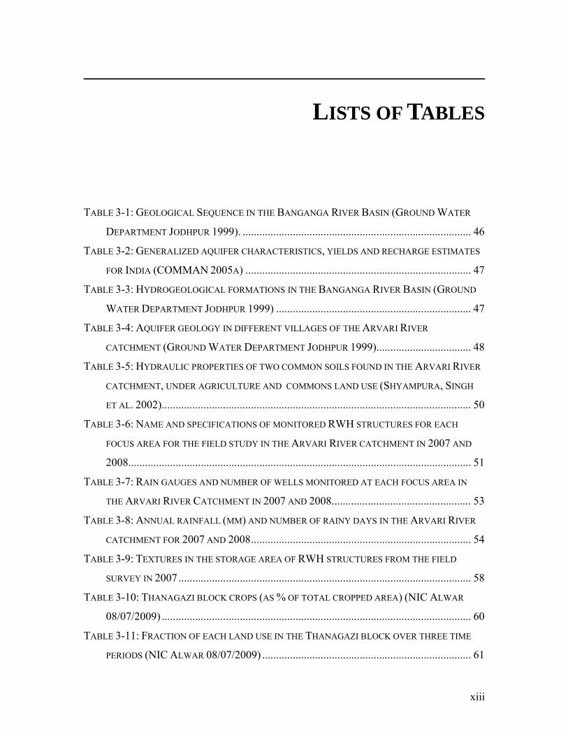
LISTS OF TABLES
TABLE 3-1: GEOLOGICAL SEQUENCE IN THE BANGANGA RIVER BASIN (GROUND WATER
DEPARTMENT JODHPUR 1999). .................................................................................. 46
TABLE 3-2: GENERALIZED AQUIFER CHARACTERISTICS, YIELDS AND RECHARGE ESTIMATES
FOR INDIA (COMMAN 2005A) ................................................................................. 47
TABLE 3-3: HYDROGEOLOGICAL FORMATIONS IN THE BANGANGA RIVER BASIN (GROUND
WATER DEPARTMENT JODHPUR 1999) ...................................................................... 47
TABLE 3-4: AQUIFER GEOLOGY IN DIFFERENT VILLAGES OF THE ARVARI RIVER
CATCHMENT (GROUND WATER DEPARTMENT JODHPUR 1999).................................. 48
TABLE 3-5: HYDRAULIC PROPERTIES OF TWO COMMON SOILS FOUND IN THE ARVARI RIVER
CATCHMENT, UNDER AGRICULTURE AND COMMONS LAND USE (SHYAMPURA, SINGH
ET AL. 2002)............................................................................................................... 50
TABLE 3-6: NAME AND SPECIFICATIONS OF MONITORED RWH STRUCTURES FOR EACH
FOCUS AREA FOR THE FIELD STUDY IN THE ARVARI RIVER CATCHMENT IN 2007 AND
2008........................................................................................................................... 51
TABLE 3-7: RAIN GAUGES AND NUMBER OF WELLS MONITORED AT EACH FOCUS AREA IN
THE ARVARI RIVER CATCHMENT IN 2007 AND 2008.................................................. 53
TABLE 3-8: ANNUAL RAINFALL (MM) AND NUMBER OF RAINY DAYS IN THE ARVARI RIVER
CATCHMENT FOR 2007 AND 2008............................................................................... 54
TABLE 3-9: TEXTURES IN THE STORAGE AREA OF RWH STRUCTURES FROM THE FIELD
SURVEY IN 2007......................................................................................................... 58
TABLE 3-10: THANAGAZI BLOCK CROPS (AS % OF TOTAL CROPPED AREA) (NIC ALWAR
08/07/2009) ............................................................................................................... 60
TABLE 3-11: FRACTION OF EACH LAND USE IN THE THANAGAZI BLOCK OVER THREE TIME
PERIODS (NIC ALWAR 08/07/2009) ........................................................................... 61

xiv
TABLE 3-12: AVERAGE PHYSICAL PARAMETERS OF RWH STRUCTURES BUILT BY TBS AND
THE COMMUNITY SINCE 1985 – 2005 IN THE ARVARI RIVER CATCHMENT (PERS COMM.
TBS).......................................................................................................................... 64
TABLE 4-1: STATISTICAL PARAMETERS FOR EQ 4-2, DESCRIBING THE RELATIONSHIP
BETWEEN AVERAGE DEPTH (M) AND REP VOLUME (M3) ON NON-RAINY DAYS TO
CALCULATE REP VOLUME (M3) ON RAINY DAYS........................................................... 71
TABLE 4-2: TUKEY HSD RESULTS OF POTENTIAL RECHARGE BY FOCUS AREA AND RWH
TYPE........................................................................................................................... 75
TABLE 4-3: AVERAGE DAILY REP (MM/DAY) AND NUMBER OF DAYS WATER STORED IN
MONITORED RWH STRUCTURES IN 2007 AND 2008 ................................................... 76
TABLE 4-4: STATISTICAL PARAMETERS FOR EQ 4-5 DESCRIBING THE RELATIONSHIP
BETWEEN THE CUMULATIVE SUM OF REP (MM) AND CUMULATIVE SUM OF RAINFALL
(MM) .......................................................................................................................... 78
TABLE 4-5: RECHARGE EFFICIENCY OF RWH STRUCTURES IN 2007 AND 2008................. 82
TABLE 4-6: GENERALISED AQUIFER CHARACTERISTICS FOR AQUIFERS ACROSS INDIA AND
MOST LIKELY OCCURRING IN THE ARVARI RIVER CATCHMENT (COMMAN 2005A). 89
TABLE 4-7: DESCRIPTION OF GEOLOGY IN AREAS WHERE MONITORED DUG WELLS............ 89
TABLE 4-8: AVERAGE RGW (MM/DAY) IN THE FOCUS AREAS IN THE ARVARI RIVER
CATCHMENT USING THE WTF METHOD.................................................................... 102
TABLE 4-9: HYDRAULIC PROPERTIES FOR SOIL IN MONITORED RWH STRUCTURES USING
THE SOIL TEXTURE TRIANGLE (CM3
WATER/CM3
SOIL) (SAXTON, RAWLS ET AL. 1986)
................................................................................................................................. 104
TABLE 4-10: EXAMPLE ANALYSIS OF MOVEMENT OF REP THROUGH THE SOIL PROFILE ON
ONE DAY IN 2008 (MM/DAY) .................................................................................... 105
TABLE 4-11: APPROXIMATE AREA OF THE CATCHMENT FOR DIFFERENT RWH STRUCTURE
TYPES IN THE ARVARI RIVER CATCHMENT AND APPROXIMATE PERCENTAGE OF
ANNUAL RAINFALL THAT BECOMES REP IN 2007 AND 2008 ...................................... 106
TABLE 5-1: STATISTICAL SUMMARY OF THANAGAZI RAINFALL (1980 – 2006) COMPARED
WITH THE MEASURED RAINFALL FROM THE ARVARI RIVER CATCHMENT AT BHAONTA
AND HAMIRPUR FOCUS AREAS IN 2007 AND 2008 (P = RAINFALL)........................... 118
TABLE 5-2: LAI FOR EACH HYDROLOGICAL RESPONSE UNIT IN THE MODEL .................. 123

xv
TABLE 5-3: DESCRIPTION OF HYDROLOGICAL RESPONSE UNITS (HRUS) IN RELATION TO
CATCHMENT CHARACTERISTICS ............................................................................... 126
TABLE 5-4: CROP SEASONS IN THE ARVARI RIVER CATCHMENT...................................... 127
TABLE 5-5: LAND USE CURVE NUMBERS IN MODEL......................................................... 132
TABLE 5-6: RELATIVE SENSITIVITY INDEX CLASSES AS DESCRIBED BY LENHART ET AL.
(2002)...................................................................................................................... 135
TABLE 5-7: SENSITIVITY OF OUTPUT FROM THE MODEL WITH RAINFALL AND INPUT
PARAMETERS ........................................................................................................... 136
TABLE 5-8: SUM OF FIELD ESTIMATES OF AVERAGE POTENTIAL RECHARGE FROM RWH AND
MODEL OUTPUT OF THE SAME FOR SIMILAR ANNUAL RAINFALL YEARS .................... 138
TABLE 5-9: NATURAL ANNUAL RECHARGE FROM THE DEVELOPED REGRESSION
(RANGARAJAN AND ATHAVALE 2000) AND THE MODEL OUTPUT FOR DIFFERENT LAND
USES......................................................................................................................... 140
TABLE 5-10: MODEL PARAMETERS AND VALUES............................................................. 143
TABLE 5-11: COMPARISON OF THE MODEL DESCRIBED IN CHAPTER 5 WITH WELL
ESTABLISHED MODELS ............................................................................................. 144
TABLE 7-1 ANALYSIS OF ARP AND THE FACTORS THAT FAVOUR COLLECTIVE ACTION
(OSTROM 1990; OSTROM 1992)............................................................................... 176

xvi
LISTS OF FIGURES
FIGURE 2-1: SCHEMATIC REPRESENTATION OF RWH FUNCTION FOR GROUNDWATER
RECHARGE ................................................................................................................. 11
FIGURE 2-2: EXAMPLE OF A RWH STRUCTURE KNOWN AS AN ANICUT IN RAJASTHAN,
INDIA. AT THE END OF THE MONSOON IN SEPTEMBER THE STRUCTURE IS FULL. THREE
MONTHS LATER THE STORAGE IS ALMOST EMPTY, THROUGH EVAPORATIVE LOSS,
LATERAL SUBSURFACE FLOW AND RECHARGE............................................................ 13
FIGURE 2-3: COMMON VILLAGE WELLS FOUND IN RAJASTHAN, WITH DIESEL PUMPS. ........ 35
FIGURE 3-1: POSITION OF THE CASE STUDY CATCHMENT, THE ARVARI RIVER CATCHMENT
(OR CATCHMENT OF SAINTHAL SAGAR DAM) IN THE EASTERN PART OF THE STATE OF
RAJASTHAN, INDIA. THE VILLAGES, WHICH WERE THE FOCUS OF THE DATA
COLLECTION STUDY, ARE HIGHLIGHTED..................................................................... 40
FIGURE 3-2: DAILY RAINFALL (MM) AT THE THANAGAZI STATION FROM 1980 – 2006 WITH
A MOVING AVERAGE LINE OVER TWO YEARS TO INDICATE ANY TRENDS (NO RAINFALL
DATA AVAILABLE FOR 1999)...................................................................................... 42
FIGURE 3-3: QUANTILE-QUANTILE PLOTS FOR DAILY RAINFALL (MM) AT THANAGAZI
STATION FOR A. 1980 – 1986 BY 1987 – 1993, B. 1992 – 1997 BY 1998 – 2002 ......... 43
FIGURE 3-4: NUMBER OF RAINFALL EVENTS GREATER THAN 35 MM AT THANAGAZI STATION
FROM 1980-2006 ....................................................................................................... 44
FIGURE 3-5: MONTHLY AVERAGE DAILY POTENTIAL EVAPOTRANSPIRATION (PREISTLEY-
TAYLOR METHOD) FOR THE ALWAR DISTRICT FROM 1901-2002 (INDIA WATER
PORTAL 2009)............................................................................................................ 45
FIGURE 3-6: POSITION OF MONITORED WELLS IN THE ARVARI RIVER CATCHMENT ........... 52
FIGURE 3-7: DAILY RAINFALL (MM) FROM RAIN GAUGES IN THE ARVARI RIVER CATCHMENT
IN 2007 AND 2008...................................................................................................... 54

xvii
FIGURE 3-8: VARIATION IN DAILY RAINFALL DEPTH INTERVALS (MM) IN THE ARVARI RIVER
CATCHMENT DURING THE MONSOON SEASON (JUNE-SEPTEMBER) OF 2007 AND 200855
FIGURE 3-9: LOCATIONS OF SAMPLED SOIL TEXTURE PROFILES EXAMINED IN THE ARVARI
RIVER CATCHMENT IN 2007 ....................................................................................... 57
FIGURE 3-10: TWO GENERAL SOIL PROFILES AND TEXTURE CHARACTERISTICS IN THE
ARVARI RIVER CATCHMENT FROM THE FIELD SURVEY UNDER THE MAIN LAND USES, A.
AGRICULTURE AND B. COMMONS .............................................................................. 58
FIGURE 3-11: A. THE DIFFERENT TYPES OF RWH STRUCTURES AND THEIR EXTENT WITHIN
THE ARVARI RIVER CATCHMENT, B. DIGITAL ELEVATION MODEL (DEM) OF THE
ARVARI RIVER CATCHMENT...................................................................................... 63
FIGURE 4-1: AFTER SHARDA ET AL. (2006), THE WATER BALANCE OF THE STORAGE OF A
RWH STRUCTURE...................................................................................................... 68
FIGURE 4-2: FITTED LINEAR MODEL TO ESTIMATE REP ON RAINY DAYS USING REP
CALCULATED FROM THE WATER BALANCE METHOD ON NON-RAINY DAYS, A. SANKARA
BANDH, B. BERUJI BANDH, C. JHIRI JOHAD, D. LALPURA JOHAD ................................. 72
FIGURE 4-3: ESTIMATED REP (M3) WITH DAILY RAINFALL (MM) FROM BHAONTA GAUGE FOR
A. SANKARA BANDH, B. BERUJI BANDH, AND WITH DAILY RAINFALL FROM HAMIRPUR
GAUGE FOR C. JHIRI JOHAD, D. LALPURA JOHAD ........................................................ 73
FIGURE 4-4: AVERAGE DEPTH (MM) BY DAILY REP (MM) FOR A. SANKARA BANDH, B. BERUJI
BANDH, C. LALPURA JOHAD, (WHERE REP (MM) IS CALCULATED BY DIVIDING REP (M3)
BY AVERAGE SURFACE AREA (M2))............................................................................. 74
FIGURE 4-5: CUMULATIVE POTENTIAL RECHARGE (MM) AGAINST CUMULATIVE RAINFALL
(MM) USING THE EXPONENTIAL FUNCTION (Y AXIS IS LOGGED) A. SANKARA BANDH, B.
BERUJI BANDH, C. JHIRI JOHAD, D. LALPURA JOHAD .................................................. 79
FIGURE 4-6: CUMULATIVE RAINFALL FOR 2007 (MM) AGAINST CUMULATIVE RAINFALL FOR
2008 (MM) (LINE REPRESENTS X = Y) ......................................................................... 80
FIGURE 4-7: CUMULATIVE RAINFALL (MM) REQUIRED FOR 1 MM, 10 MM AND 100 MM OF REP
FOR EACH MONITORED RWH STRUCTURE AND COMPARED WITH ESTIMATES FROM
SHARDA ET AL. (2006) ............................................................................................... 81
FIGURE 4-8: DAILY DISCHARGE OR OVERFLOW OVER THE MONITORED ANICUTS ON THE
ARVARI RIVER IN 2007 AND 2008.............................................................................. 83

xviii
FIGURE 4-9: CUMULATIVE SUM OF RAINFALL (MM) AT HAMIRPUR AGAINST CUMULATIVE
SUM OF OVERFLOW ON THE ANICUTS ON THE ARVARI RIVER AT A. HAMIRPUR, B.
KALED, C. NITATA ..................................................................................................... 85
FIGURE 4-10: ESTIMATED REP (MM/DAY) FROM MONITORED ANICUTS ON THE ARVARI RIVER
IN 2007 AND 2008...................................................................................................... 86
FIGURE 4-11: MEASURED EC (MS/CM-1) VALUES IN ANICUTS AND DUG WELLS IN 2008 IN
THE FOCUS AREAS OF A. KALED , B. NITATA, C. HAMIRPUR ....................................... 87
FIGURE 4-12: THE SIX MONITORED WELLS AT FOCUS AREA BHAONTA, A. ASL (M)
GROUNDWATER LEVEL, B. RELATIVE GROUNDWATER LEVEL HEIGHT, C. RELATIVE
GROUNDWATER LEVEL HEIGHT AT WELL BK5 AND DEPTHS AT SANKARA BANDH AND
BERUJI BANDH (M) ..................................................................................................... 91
FIGURE 4-13: THE TWO MONITORED DUG WELLS AT FOCUS AREA LALPURA, A. ASL (M)
GROUNDWATER LEVEL, B. RELATIVE GROUNDWATER LEVEL HEIGHT (M) .................. 92
FIGURE 4-14: THE MONITORED WELL AT JHIRI ASL GROUNDWATER LEVEL (M)................ 93
FIGURE 4-15: THE FOUR MONITORED DUG WELLS AT HAMIRPUR A. GROUNDWATER LEVEL
ASL (M), B. RELATIVE GROUNDWATER LEVEL HEIGHT (M)........................................ 94
FIGURE 4-16: RESPONSE OF MONITORED WELLS AT KALED A. GROUNDWATER LEVEL ASL
(M), B. RELATIVE GROUNDWATER LEVEL HEIGHT (M), C. RELATIVE GROUNDWATER
LEVEL HEIGHT (M) WELL KLD6 ................................................................................. 95
FIGURE 4-17: RESPONSE OF TWO MONITORED DUG WELLS AT NITATA, A. GROUNDWATER
LEVEL ASL (M), B. RELATIVE GROUNDWATER LEVEL HEIGHT (M)............................. 96
FIGURE 4-18: ROADSIDE WELLS BETWEEN JHIRI AND KALED. A. GROUNDWATER LEVEL
ASL (M), B. RELATIVE WATER LEVEL HEIGHT (M) ..................................................... 96
FIGURE 4-19: MONITORED DUG WELLS ALONG ROADSIDE FROM JHIRI TO LALPURA A.
GROUNDWATER LEVEL ASL (M), B. RELATIVE WATER LEVEL HEIGHT (M) ................ 97
FIGURE 4-20: INVERSE DISTANCE WEIGHTED INTERPOLATION OF MONITORED WELL
HEIGHTS ASL (M) A. 1ST JUNE 2007, B. 12 SEPTEMBER 2007 ..................................... 99
FIGURE 4-21: INVERSE DISTANCE WEIGHTED INTERPOLATION OF MONITORED WELL
HEIGHTS ASL (M) A. 1ST JUNE 2008, B. 12 SEPTEMBER 2008 ..................................... 99
FIGURE 4-22: INTERPOLATION OF AVERAGE RGW (MM/DAY) FROM WTF METHOD IN A.
2007, B.2008............................................................................................................ 100

xix
FIGURE 4-23: DIGITAL ELEVATION MODEL (DEM) FOR THE AREA OF THE MONITORED DUG
WELLS ...................................................................................................................... 102
FIGURE 4-24: COMPARISON OF REP ESTIMATES FROM MONITORED RWH (MM/DAY) AND RGW
IN MONITORED DUG WELLS (MM/DAY) IN 2007 AND 2008........................................ 104
FIGURE 5-1: DIVISION OF SUBBASINS, BASED ON THE ARVARI RIVER CATCHMENT, IN THE
MODELLED CATCHMENT OF THE DEVELOPED CONCEPTUAL HYDROLOGICAL MODEL 114
FIGURE 5-2: CROSS CORRELATION FUNCTION FROM POTENTIAL RECHARGE (REP) FROM
SANKARA BANDH TO ACTUAL RECHARGE (RGW) AT WELL BK1 ............................... 116
FIGURE 5-3: STOCHASTIC RAINFALL MODELLING FLOW CHART BASED ON FERNANDEZ-
ILESCAS AND RODRIGUEZ-ITURBE (2004) AND USED IN THIS MODEL TO PREDICT DAILY
RAINFALL FOR EACH SUBBASIN ................................................................................ 117
FIGURE 5-4: RELATIONSHIP BETWEEN ANNUAL RAINFALL AND MONSOON SEASON
RAINFALL, AND DRY SEASON RAINFALL (MM) AT THANAGAZI RAINFALL STATION
(1980 – 2006) .......................................................................................................... 119
FIGURE 5-5: HISTOGRAM OF THE ALWAR ANNUAL RAINFALL DISTRIBUTION 1901 – 2002
INDICATING A LOG NORMAL DISTRIBUTION .............................................................. 119
FIGURE 5-6: A. ONE SIMULATION OF MODELLED ANNUAL RAINFALL USING THE FOURIER
SERIES FUNCTION (RED) AND WITH A RANDOM COMPONENT (BLUE) COMPARED WITH
ALWAR ANNUAL RAINFALL (BLACK), B. QUANTILE-QUANTILE PLOT OF ONE
SIMULATION OF MODELLED ANNUAL RAINFALL AGAINST OBSERVED ANNUAL
RAINFALL (MM) (WITH LINE X = Y), C. EXAMPLE OF ONE SIMULATION OF MODELLED
ANNUAL RAINFALL DISTRIBUTION. THE COLOURED POINTS REPRESENT COLLECTED
RAINFALL DURING THE FIELD STUDY FROM THE THREE GAUGES IN THE CATCHMENT IN
2007 AND 2008 (SECTION 3.2.2) .............................................................................. 121
FIGURE 5-7: WATER BALANCE FOR AGRICULTURE HRUS ............................................... 128
FIGURE 5-8: WATER BALANCE FOR RWH HRUS............................................................ 129
FIGURE 5-9: SCHEMATIC REPRESENTATION OF ONE SUBBASIN IN THE MODEL WITH
DIFFERENT HRUS IN THE SOIL LAYER ...................................................................... 133
FIGURE 5-10: COMPARISON OF CUMULATIVE SUM OF RAINFALL AGAINST CUMULATIVE SUM
OF RECHARGE BETWEEN A. FIELD RESULTS AND B. MODEL OUTPUT ........................ 139

xx
FIGURE 5-11: GROUNDWATER LEVELS IN A. FIELD WELL KLD6 2008 IN VILLAGE KALED
(MM ASL), B. FROM THE MODEL OUTPUT IN A SIMILAR RAINFALL YEAR IN SUBBASIN 1
................................................................................................................................. 140
FIGURE 5-12: A. DAILY DISCHARGE OVER ANICUTS ON THE ARVARI RIVER IN 2007 AND
2008 (M3), B. DAILY STREAMFLOW FROM MODEL OUTPUT (MM) .............................. 141
FIGURE 6-1: HISTOGRAM OF ANNUAL RAINFALL DISTRIBUTION (MM) FOR 30 REALISATIONS
OF 12 YEAR MODEL SIMULATIONS IN SUBBASIN 2 .................................................... 151
FIGURE 6-2: DISTRIBUTION OF THE SUSTAINABILITY INDICES, WITH MEDIAN, FOR DIFFERENT
AREAS OF IRRIGATION WITHOUT RWH FOR KHARIF AND RABI A. RELIABILITY INDEX,
B. RESILIENCE INDEX, C. VULNERABILITY INDEX .................................................... 154
FIGURE 6-3: DISTRIBUTION OF THE RELIABILITY INDEX WITH MEDIAN FOR DIFFERENT
AREAS OF IRRIGATION AND RWH FOR KHARIF AND RABI SEASON............................ 155
FIGURE 6-4: DISTRIBUTION OF THE RESILIENCE INDEX WITH MEDIAN FOR DIFFERENT AREAS
OF IRRIGATION AND RWH FOR KHARIF AND RABI SEASON ....................................... 157
FIGURE 6-5: DISTRIBUTION OF THE VULNERABILITY INDEX WITH MEDIAN FOR DIFFERENT
AREAS OF IRRIGATION AND RWH FOR KHARIF AND RABI SEASON............................ 158
FIGURE 6-6: RELIABILITY IN RABI WITH BELOW AVERAGE RAINFALL AND ABOVE AVERAGE
RAINFALL A. WITHOUT RWH AT VARIOUS LEVELS OF IRRIGATION, B. WITH VARIOUS
SCENARIOS OF RWH AND IRRIGATED AGRICULTURE ............................................... 160
FIGURE 6-7: RESILIENCE IN RABI WITH BELOW AVERAGE RAINFALL AND ABOVE AVERAGE
RAINFALL A. WITHOUT RWH AT VARIOUS LEVELS OF IRRIGATION, B. WITH VARIOUS
SCENARIOS OF RWH AND IRRIGATED AGRICULTURE ............................................... 161
FIGURE 6-8: VULNERABILITY IN RABI WITH BELOW AVERAGE RAINFALL AND ABOVE
AVERAGE RAINFALL A. WITHOUT RWH AT VARIOUS LEVELS OF IRRIGATION, B. WITH
VARIOUS SCENARIOS OF RWH AND IRRIGATED AGRICULTURE ................................ 162
FIGURE 6-9: SUSTAINABILITY INDICES IN SIMULATIONS WITH A. 2 YEAR DROUGHT PERIOD,
B. 4 YEAR DROUGHT PERIOD, C. 6 YEAR DROUGHT PERIOD ....................................... 163
FIGURE 6-10: ANNUAL STREAMFLOW AS % OF ANNUAL RAINFALL (MM) A. NO RWH OR
IRRIGATED AGRICULTURE, B. 15% IRRIGATED AGRICULTURE, NO RWH, C. 15%
IRRIGATION, 0.5% RWH, D. 15% IRRIGATION, 3% RWH, E. 5% IRRIGATION, 3%
RWH, F. 10% IRRIGATION, 3% RWH...................................................................... 165

1
1. INTRODUCTION
1.1. Motivation
Water is the most basic necessity for nature and humans. However, as human population
increases, society is facing serious issues related to water quantity and quality. The
global community now acknowledges a water crisis: the UN has declared 2005 – 2015
the decade of water and many of the Millennium Development Goals focus on water;
Target 10 is to halve the proportion of people without sustainable access to safe drinking
water and basic sanitation by 2015 (UN Millennium Project 2005).
Groundwater is an important resource for humans. Globally groundwater provides 50%
of current potable water supplies, 40% of the demand for self-supplied industry and 20%
of irrigation water (Villholth 2006). In India, where 15% of the world’s population lives,
groundwater accounts for over 80% of domestic water use in rural areas, and 55 – 60% of
the Indian population (about 620 million people) is directly or indirectly dependent on
groundwater for its livelihood. Since the increased use of groundwater in India, millions
of people have been lifted out of poverty (Kemper 2007). Despite and because of the
importance of groundwater, exploitation and degradation of groundwater supplies is a
serious issue in India, and groundwater tables are rapidly falling in a number of states

2
(Rodell, Velicogna et al. 2009). The search for feasible solutions for sustaining
groundwater stores is therefore gaining considerable momentum, and rainwater
harvesting (RWH) is encouraged as a possible solution.
Rainwater harvesting (RWH), a traditional catchment development tool in South Asia,
collects and stores runoff that falls during the heavy downpours in the Indian monsoon
season, allowing time for the stored water to recharge shallow groundwater aquifers.
Despite the so-called ‘groundwater recharge movement’ in India, which has been
promoting and reinvesting in RWH over the past three decades, there is a lack of
systematic studies that have measured the hydrological impact of RWH structures and
generated recharge on local and catchment-scale water balances. A number of studies
have highlighted the possible negative impacts of RWH, which could be high
unreliability in drought years and high negative externalities at higher degrees of
catchment development (Kumar, Patel et al. 2008). Rainwater harvesting redistributes
the available water resources across the catchment, by increasing the annual amount of
catchment rainfall that is stored and becomes recharge, which could change other water
balance components, including evaporation and streamflow, with possible trade-offs
between upstream and downstream users, and users and the environment (Kumar, Ghosh
et al. 2006). However these arguments are not confirmed by any empirical studies.
The purpose of this research is therefore to expand the knowledge of the impacts of RWH
at the local and catchment-scales. This research seeks to understand the changes in the
catchment water balance by first examining the local-scale impacts of RWH in a case
study catchment of the Arvari River in the state of Rajasthan, India. A simple conceptual
model is subsequently developed to extrapolate the results of the field work to the
catchment-scale. This model makes it possible to investigate the interrelationships
between RWH, irrigated agriculture and any possible impacts on catchment water
balances that may occur under increasing areas of RWH. The major contribution from
this study is a methodology to systematically examine the impact of RWH development
in a catchment.

3
1.2. Research Questions and Objectives
The principal question investigated in this thesis is:
What are the hydrological impacts of RWH at the local and the catchment-scales?
This research question will be broken down into two main parts. The first section
considers the local-scale impacts of RWH for a case study catchment, the Arvari River,
and the second section examines the catchment-scale impacts through the use of a water
balance model. A final smaller section examines the institution in the study area
catchment that manages groundwater use.
The hypotheses that are tested in the first section are:
Recharge from RWH has a large local-scale effect on groundwater levels
The magnitude of recharge from RWH is dependent on the annual rainfall
To test these hypotheses at the local-scale, research questions addressed included:
How much rainfall is potentially recharged by an individual structure?
Are there any differences or similarities in recharge behaviour between
structures in a similar area or by structure type?
How much potential recharge reaches the underlying aquifer?
How effective is RWH in recharging groundwater?
What is the zone of influence of RWH?
What are the main hydrological processes that are influenced by RWH?
What are the general climatic and landscape characteristics of the semi-arid
case study catchment that might influence RWH?
The hypotheses that are tested in the second section are:
Increased area of RWH decreases streamflow downstream
Development of RWH increases the viability of irrigated agriculture
At higher levels of RWH development in a catchment, the benefit is not as
great as during the initial stages of RWH construction.
To address these hypotheses the research questions considered were:

4
Is there an existing water balance model that can simulate all the relevant
catchment hydrological processes related to RWH?
Using a hydrological model, how does RWH impact the modelled catchment
system?
How effective is RWH in alleviating drought for groundwater irrigated
agriculture?
Rainwater harvesting is a supply-side groundwater management tool, and therefore the
institutions, which define access and conservation rules, are important to consider for
sustainable groundwater management. In the final section of the thesis, the effectiveness
of the catchment community institution in the case study catchment is investigated, and
whether this institution addresses groundwater demand issues.
1.3. Outline of Thesis
The study consists of eight chapters. Following this Introduction, Chapter 2 reviews the
current literature related to RWH in the world and more specifically in India. The major
issues with groundwater in India are considered and RWH is defined. The gaps in the
literature are identified and relate to the quantification of RWH impacts at the local-scale
and catchment-scale. Groundwater institutions in India are also highlighted as an under
researched area.
Chapter 3 gives a brief introduction to the study area catchment, the Arvari River, which
was chosen for extensive field work in 2007 and 2008. The catchment is well known for
its RWH work, with over 366 structures throughout the catchment. Like many
catchments in India, RWH development was planned at the village-scale, with no larger
catchment-scale plans. There is limited data available on aquifer characteristics, and no
climate station in the catchment. The methodology for data collection is also described

5
and the analysis of the variation in catchment rainfall presented. The dominant land uses
are explained and details of sampled soil profiles are given.
Field data collected in the monsoons of 2007 and 2008 in the Arvari River catchment are
analysed in Chapter 4. The first part of the chapter examines the data from the RWH
structures and calculates potential recharge from each monitored structure. These results
are compared with the analysis of the response in groundwater levels from the monitored
dug wells. High spatial and temporal variability is seen; a common feature of semi-arid
regions, but some broad conclusions on local-scale RWH impacts can be inferred from
this chapter. This information is needed to up-scale these impacts to a catchment-scale
water balance model.
Chapter 5 develops a conceptual water balance model, which will be used to answer the
catchment-scale research questions. The model is based on hydrological response units
(HRUs), and includes the surface water – groundwater interactions, which are important
in RWH function. Results of the simulation of different management scenarios in the
model are then compared in Chapter 6 using sustainability indices. The impact of rainfall
on RWH function is also examined.
Chapter 7 examines the Arvari River Parliament, a catchment group in the case study
area, which has defined informal rules for water resource development and management.
These rules are considered with regards to groundwater use, and whether the institution is
effective in monitoring and enforcing groundwater extraction.
The final chapter presents the important implications of the results. Here, key findings
are summarised, and implications are drawn from the study’s findings. The chapter also
discusses limitations of the study, leading to avenues for further research.

6
2. A REVIEW OF RAINWATER
HARVESTING (RWH) FOR
GROUNDWATER RECHARGE
2.1. Introduction
Globally groundwater is an increasingly important natural resource, particularly in India
where it accounts for more than 45% of the total irrigation supply (Kumar, Singh et al.
2005), and for about 9% of India’s GDP (Mudrakartha 2007). However this has not
always been the case, in the last 50 years or so India has seen a huge boom in the use of
groundwater. In 1960, tube wells numbered less than one million, which by 2000 had
increased to an estimated 19 million (Shah, Deb Roy et al. 2003). This has had a large
impact on small-holder farmers in India, because crops irrigated by groundwater are
generally more productive than using surface water irrigation as groundwater requires
little transport, can be accessed relatively easily and cheaply, is produced where it is
needed and provides a relatively reliable source of water (Dhawan 1995). Evidence from
India suggests that crop yield/m3 on groundwater irrigated farms tends to be 1.2 – 3 times

7
higher than on surface water irrigated farms (Dhawan 1989). However three serious
problems currently affect groundwater use in South Asia: depletion due to overdraft;
water logging and salinisation; and pollution due to agricultural, industrial and other
human activities (Shah, Deb Roy et al. 2003). In many parts of the country the water
table is declining at the rate of 1 − 2 m/year (Singh and Singh 2002). The search for
feasible solutions for alleviating groundwater shortages is therefore becoming urgent.
One option being increasingly considered and implemented, is rainwater harvesting
(RWH) (Agarwal and Narain 1997).
Different techniques of rainwater harvesting are found throughout the Middle East,
Africa and South Asia. In many areas of India this method is important for groundwater
recharge, because the major portion of the annual rainfall is received in around 100 hours
of heavy monsoonal downpour, providing very little time for natural recharge to the
aquifer due to rapid runoff. This technique has become even more relevant as more land
has been deforested, increasing runoff. Rainwater harvesting stores monsoonal runoff,
which then percolates to groundwater tables (Keller, Sakthivadivel et al. 2000). India has
a long history of RWH and currently rising investment in RWH development. It is
therefore increasingly important to quantify the hydrological impact of RWH structures.
In particular, it is important to understand the downstream trade-offs in a larger
catchment with RWH, because of possible changes in the catchment water balance and
changes between blue and green water (Falkenmark 2003).
While RWH addresses supply issues related to groundwater, the management of
groundwater demand is through institutions. Institutions affect the access, operation and
monitoring of a resource through defined rules. Historically natural resources were
common property in India, but under present legislation groundwater rights are
privatised. This has lead to property rights issues and over-extraction of groundwater, for
example the Coca Cola case in India, where the industrial use of groundwater has caused
water levels to decline in neighbouring small-holder farms (Gronwall 2006). In
developing countries community-based common property resource management is a
viable alternative to state or private property rights (Saleth 2005). A key question is

8
whether such community institutions would be effective in management of the
groundwater resource.
2.2. Rainwater harvesting (RWH)
Rainwater harvesting involves using small-scale structures to collect runoff for either
supplemental irrigation, as is most common in Africa (Ngigi, Savenije et al. 2007), or for
groundwater recharge, as is typical in many regions of India (Kumar, Ghosh et al. 2006).
Although literature highlights RWH as an efficient cost-effective method of replenishing
aquifers, the few studies that have quantified RWH impacts have generally done so at
local, small-scale catchments and have not considered larger catchment hydrological
impacts, such as downstream trade-offs or surface water – groundwater interactions,
where use of one type affects the availability of the other (Badiger, Sakthivadivel et al.
2002; Sharda, Kurothe et al. 2006).
2.2.1. Groundwater Use and Problems in India
Eighty percent of global groundwater use occurs in Bangladesh, China, India, Iran,
Pakistan and the US (Shah, Burke et al. 2007), with India being the largest groundwater
irrigator in the world (Shah, Singh et al. 2006). In India and China combined, 1 – 1.2
billion poor small-holder farmers are supported by groundwater (Shah, Burke et al.
2007). This is because groundwater irrigation tends to be less biased against the poor
than large scale surface water irrigation projects (Deb Roy and Shah 2002). Groundwater
is easily accessible and can be developed quickly by farmers or small groups, and can be
reliable and flexible in time and space. In India groundwater-based irrigation covers a
greater area than the established canal irrigated systems, which were set up largely by the
colonial government in the late 19th century (Sakthivadivel 2007; Shah 2007a).
Groundwater also has the advantage of having less evaporation than surface dams and
canals (Keller, Sakthivadivel et al. 2000).

9
In India, the advance of technology from shallow wells with animal pulling and human
labour, to diesel pumps and electricity has greatly impacted the amount of groundwater
extraction since independence in 1947 (Shah, Singh et al. 2006). While exponential
groundwater use over the past few decades has improved livelihoods by allowing more
stability for cropping, there are increasingly serious issues with aquifer depletion (Shah,
Burke et al. 2007). This is partly due to electricity subsidies by state-owned electricity
services to farmers, which has encouraged over extraction of groundwater (Radhakrishna
2003; Narasimhan 2005; Subash Chandra 2005). But there is also a serious lack of
proper planning and management of groundwater extraction, with little regulation and
enforcement (Radhakrishna 2003; Datta 2005; Subash Chandra 2005). Groundwater is
largely a private informal sector, where each well owner regulates their own use; public
agencies do not play a direct role in groundwater management. Effective institutional
arrangements to manage groundwater have not yet been developed, which means that use
of groundwater still remains unchecked (Villholth and Giordano 2007; Shah 2007b) (this
will be explored in more detail in Section 2.4). With the increasing severity of extreme
events such as droughts and floods predicted over the next 20 years, and increasing
population pressures, groundwater management will become even more important to
address (Pandey, Gupta et al. 2003; Gupta and Deshpande 2004; Ramesh and Yadava
2005).
Currently the response to groundwater depletion has focussed on supply-side
management of groundwater rather than demand-side. In India a massive integrated
catchment development program provides public resources to local communities for
catchment development works, including constructing rainwater harvesting (RWH)
structures (Hope 2007; Shah 2007a). Based on trends during the 1990’s, there has been a
progressive shift of budgetary allocations from irrigation development to RWH (Shah
2007a). Methods to recharge aquifers, including RWH (sometimes referred to as
artificial recharge), have become so widespread in India over the last two to three
decades that it is now referred to as ‘a groundwater movement’ or ‘artificial recharge
movement’ (Sakthivadivel 2007; Sakthivadivel 2008). However one of the difficulties of

10
such a movement is the lack of documentation of the impacts of these projects on
groundwater, and any upstream-downstream trade-offs (Hope 2007; Sakthivadivel 2008).
The reliance and depletion of groundwater in India has meant investment in RWH, to
augment groundwater stores, has occurred rapidly without any hydrological assessment
(Kumar, Ghosh et al. 2006). Consequently, the use of RWH and its impacts must be
more fully understood to allow its potential benefits and impacts to be realised.
2.2.2. What is Rainwater harvesting (RWH)?
Some of the literature describes RWH for groundwater recharge as artificial recharge
(Bouwer 2002). However in much of the literature, RWH is considered part of ‘managed
aquifer recharge’, which also includes artificial recharge, enhanced recharge, water
banking and sustainable underground storage (Dillon 2005; Gale 2005). Managed
aquifer recharge is defined as the ‘planned, human activity of augmenting the amount of
groundwater available through works designed to increase the natural replenishment or
percolation of surface waters into the groundwater aquifers, resulting in the
corresponding increase in the amount of groundwater available for abstraction’ (IETC
1998).
Rainwater harvesting encompasses methods to induce, collect, conserve, and store runoff
from various sources and purposes, by linking a runoff-producing area with a separate
runoff-receiving area (Boers and Benasher 1982; Rockstrom 2000; Young, Gowing et al.
2002) (Figure 2-1). Methods of RWH have three common characteristics (Boers and
Benasher 1982):
1. They depend upon small-scale capture of local water. RWH does not include
storing river water in large reservoirs or the mining of groundwater.
2. They can be applied in arid and semi-arid regions, where runoff has an
intermittent character and rainfall is highly variable, so drought and flood hazards
to agriculture are significant. In these areas storage of water is important. This
means RWH is viable in areas with annual rainfall as low as 300 mm (Kutch

11
1982), but this may also be a disadvantage, because RWH is dependent on limited
and uncertain rainfall (Qadir, Sharma et al. 2007).
3. Rainwater harvesting is a relatively small-scale operation in terms of catchment
area, volume of storage, and capital investment. The scale of RWH can range
from household, to field or small catchment (Ngigi 2003). Mbilinyi, Tumbo et al.
(2005) based RWH on the size of the runoff-producing area. These include;
On-farm, within-field systems or in situ. Rainfall is captured where it
falls, to conserve water and prevent runoff from cropped areas and prolong
the time for infiltration (Vohland and Barry 2009).
Micro-catchment system, where there is a distinct division between the
runoff-generating catchment area and a cultivated basin or storage area
where the runoff is concentrated and stored (Gowing, Mahoo et al. 1999).
In micro-catchment water harvesting, the percentage of runoff increases
with decreasing catchment size due to reduced infiltration losses. Small
watersheds can produce runoff of about 10 – 15% of annual rainfall (Boers
and Benasher 1982).
Macro-catchment RWH which has a large catchment area than micro-
catchment systems.
Figure 2-1: Schematic representation of RWH function for groundwater recharge

12
From as early as 4500 BC, RWH has been practised in various parts of the world (Verma
and Tiwari 1995), and is most commonly found in developing countries due to its
decentralised, low cost and local-scale aspects (Ngigi 2003). Indigenous RWH systems,
such as jessour and meskat in Tunisia (Schiettecatte, Ouessar et al. 2005), tabia in Libya,
cisterns in north Egypt, hafaer in Jordan, Syria and Sudan, underground cisterns (aljibes)
in Spain (Van Wesemael, Poesen et al. 1998) and many other techniques are still in use
(Oweis, Hachum et al. 1999). Irrigation reservoirs or tanks have been in existence for
more than 2000 years in Sri Lanka (Matsuno, Tasumi et al. 2003).
In India RWH also has a long history, practised for at least the last 1000 years and based
on traditional knowledge and collaboration between communities with local kings
(Agarwal and Narain 1997; Shah 2001; Pandey, Gupta et al. 2003; Sakthivadivel 2007).
Traditional RWH systems were even practised in the Indus valley (3000 BC – 1500 BC)
(Grey and Sharma 2005). Techniques of RWH have been noted in ancient texts, such as
the Rigveda (1500 BC) and the Atharva Veda (800 BC) (Agarwal and Narain 1997).
According to a historical study by Pandey, Gupta et al. (2003), abrupt climate
fluctuations heightened construction efforts of RWH structures across regions in
prehistoric and early historic societies. Despite the traditional use of RWH, it became
neglected from the time of British rule (Radhakrishna 2003). With Indian independence,
the state became the major provider of water, replacing communities and households as
the primary units for provision and management of water (Agarwal and Narain 1999).
But in the last few decades, RWH has seen a strong revival due to groundwater depletion,
involving the participation of communities, government and non-government
organizations (NGOs). It has been estimated that in India today, almost 1.5 million
traditional village tanks, ponds and earthen embankments harvest rainwater in 660 000
villages (Pandey, Gupta et al. 2003).
In India one of the main purposes of RWH is to store runoff to recharge shallow
groundwater aquifers (Agarwal and Narain 1997). This technique developed as a result
of the pattern of monsoonal rainfall in June to September of each year, but methods are
highly location specific (Verma and Tiwari 1995). The normal duration of the monsoon

13
in India is about 100 – 120 days and the Indian plains receive about 80% of annual
rainfall during this time (Kumar, Singh et al. 2005; Ramesh and Yadava 2005). As a
result of high intensity rainfall in such a short period of time, RWH stores runoff that
could otherwise continue downstream. Because RWH has a small storage capacity, it
responds quickly to rainfall-runoff compared to larger dams. Depending on the geology,
stored water can percolate into the underlying groundwater table (Figure 2-2). The
groundwater is subsequently used for irrigation, and domestic purposes via dug wells or
tube wells. A disadvantage of RWH is that open storages are often subject to high
evaporation losses, due to high surface area to volume ratios (Neumann, MacDonald et
al. 2004). But storage in aquifers has the advantage of essentially zero evaporation
(Bouwer 2002). Rainwater harvesting also tends to lead to increased crop production
intensities and greater crop yield, because rises in the water table mean better
accessibility and yields of groundwater (Keller, Sakthivadivel et al. 2000).
Figure 2-2: Example of a RWH structure known as an Anicut in Rajasthan, India. At the end of the monsoon in September the structure is full. Three months later the storage is almost empty, through evaporative loss, lateral subsurface flow and recharge.
2.2.3. Previous Studies Measuring the Impact of RWH
Until recently RWH was seen as a totally benign technology (Batchelor, Rama Mohan
Rao et al. 2003). This is because the impact of an individual dam was considered
relatively small. However the cumulative impact of RWH, which are essentially small
farm dams, on streamflows could be significant (Calder, Gosain et al. 2006).
Additionally, as groundwater increases, land use changes and favours more irrigated
September 2006 December 2006

14
agriculture (Sharma 2002). The need to quantify the overall impact of RWH in a
catchment is important, because it can cause unintended impacts such as inequitable
sharing of water between upstream and downstream users (Batchelor, Singh et al. 2002).
Nevertheless there are very few published studies that have accurately quantified the
nature and magnitude of these impacts in India, with most being mainly site-specific and
descriptive (Kumar, Ghosh et al. 2006; Sakthivadivel 2008). In addition the studies relate
mainly to RWH storage, but there is lack of research on recharge or streamflow impacts.
A number of studies have examined the amount of runoff that can be captured by RWH,
i.e. runoff potential, to prioritise catchments for RWH development. Many studies
encouraged the use of satellite images and GIS to estimate runoff potential of studied
catchments (Sharma, Kiran et al. 2001; Anbazhagan, Ramasamy et al. 2005; Sekar and
Randhir 2007). Gupta et al (1997) used the curve number (CN) method with GIS to
estimate runoff potential in a semi-arid catchment of Rajasthan for RWH development.
Tripathi and Pandey (2005) used an estimated runoff coefficient of 0.8 to examine if
villages in the Kutch District of Gujarat would benefit from RWH or not. None of these
studies considered potential RWH impacts on groundwater levels and surface flow in the
catchments they prioritised, or how many structures would be suitable without
significantly altering the catchment water balance.
Lumped or conceptual water balance models have been used to estimate groundwater
recharge from different RWH techniques in the world (Hassan and Bhutta 1996; Ouessar,
Sghaier et al. 2004; Badarayani, Kulkarni et al. 2005; Pretorius, Woyessa et al. 2005;
Ouessar, Bruggeman et al. 2008), in addition to numerical and analytical techniques
(Sorman and Abdulrazzak 1993; Khazai and Spank 1997; Kahlown and Abdullah 2004;
Jha and Peiffer 2005). Neumann et al. (2004) developed a conceptual methodology to
calculate recharge from RWH structures using Darcy’s Law, and analysed theoretical
aquifer impacts using MODFLOW. The study concluded that the impact of RWH on
water levels in a catchment may be minimal for all but the immediate vicinity of the
structure itself. Decline rates in RWH depths was suggested as an indicator for the
structures efficiency in recharging the aquifer, varying from as low as 3.5 mm/day (which

15
indicates evaporative losses), and as high as 51 mm/day. Streamflow impacts were not
considered. Other studies specific to India have focused on measurements from wells to
infer recharge from RWH. Badiger et al. (2002) monitored 42 wells in four micro-
catchments and the impact of recharge with distance from the wells. They inferred that
recharge from RWH was about 3 – 8% of rainfall. Gontia and Sikarwar (2005) reported
that groundwater levels rose by 8 m in wells in the Saurashtra region of Gujarat and this
rise was assumed to come from RWH, though no measurements were taken from the
structures themselves. Gore et al. (1998) quantified the effects of RWH in 16 observation
wells in Maharashtra state, by modelling groundwater coupled with a water balance
model, concluding that there was an overall increase in groundwater from RWH recharge
of 8 ha.m/year. In the foothills of northern India, field studies over 10 years showed the
possibilities of RWH to reduce the impact of severe droughts on agriculture, but in this
instance water stored in structures was directly used for irrigation, rather than for
percolation (Grewal, Mittal et al. 1989). Sharda et al. (2006) quantified recharge from a
number of RWH structures in Gujarat, using the water balance method and the water
table fluctuation method. They found that structures had a limited capacity to induce
maximum recharge, and that a cumulative rainfall of 104.3 mm was required to induce 1
mm of recharge.
Apart from the modelling studies by Gore et al. (1998), Neumann et al. (2004) and the
field analysis by Badiger et al (2002) and Sharda et al. (2006), there are few other studies
that have quantified the impacts of RWH in India, and of those, none considered
streamflow impacts at a larger catchment scale. Despite the positive impact RWH brings
for irrigated agriculture by increasing groundwater availability, there is a serious lack of
understanding of catchment-scale impacts of RWH, and this has been acknowledged in
many papers (Barah 1996; Kumar, Ghosh et al. 2006; Sakthivadivel 2007; Shah 2007a;
Kumar, Patel et al. 2008). There is a need for improved understanding of how RWH
functions and the impact RWH structures have on groundwater availability, as well as on
the local and downstream environment (Gale 2005). Data is sparse; therefore extensive
data collection through hydrological instrumentation is also needed. Data will then aid in

16
the use of water balance models that can extrapolate RWH impacts to a larger catchment
scale.
2.2.4. Methods for Measuring RWH Impact
Quantifying groundwater recharge is important to measure RWH impacts and is also
necessary for sustainable groundwater resource management in semi-arid and arid areas,
where groundwater resources are economically important (de Vries and Simmers 2002).
But recharge is one of the most difficult components of the water balance to measure,
because it needs to be measured below the visible surface and is highly variable;
particularly in arid environments, where it can be the smallest component of the water
balance (Bond 1998). All well-established recharge-estimation methods have limitations,
most of which yield results that are problem and scale dependent (de Vries and Simmers
2002). To quantify the impact of RWH, it is necessary to estimate the amount of runoff
stored, evaporation loss, subsequent recharge that reaches the groundwater table and
possible overflow from the structure. Recharge from RWH can be estimated using
physical measurements at the local-scale for an individual structure. However
considering the difficulty and time required for physical measurements of recharge,
modelling provides a cheaper, faster way to consider larger scale catchment effects of
RWH.
2.2.4.1. Physical Methods for measuring Recharge
Groundwater recharge is the movement of water beyond the root zone that reaches the
underlying aquifer (Bond 1998). Potential recharge (Rep) is that water which moves
below the root zone, while actual recharge (Rgw) is that water which enters the
groundwater table. The root zone is a specified depth that varies with many factors
including plant species and variety, stage of growth, crop vigour, soil conditions and
watertable conditions (de Vries and Simmers 2002; Humphreys, Edraki et al. 2003).

17
There are several physical methods for estimating recharge based on soil physical
principles and techniques. These methods attempt to directly estimate recharge, which is
a difficult, time-consuming and expensive task, because soil is spatially variable and
hence large numbers of values are required to measure a distribution (Shaw 1988). Most
of the methods are based on the water balance. The steady state water balance is based
on the law of conservation of mass, with hydrological inputs and outputs of the root zone
represented by the following equation, which can be rearranged to calculate recharge (Eq
2-1).
epS I P Roff ET R Eq 2-1
∆S = change in soil water content, I = irrigation, P = precipitation, Roff = runoff,
ET = evapotranspiration, Rep = potential recharge (recharge below the root zone).
For dynamic calculations (i.e. varying in time) saturated soil water movement is often
described by Darcy’s Law (Eq 2-2).
s
HKq
Eq 2-2
q = flux density, K = hydraulic conductivity,
s
H
= hydraulic gradient or change in hydraulic head H (m) over distance s (m)
Darcy’s Law applies if the water flow is laminar and only describes steady or stationary
flow processes, in which the flux remains constant and equal over the time step
considered (Hillel 1998). Combining Darcy’s Law with the water balance for a soil unit
allows dynamic calculation of fluxes. Extension to unsaturated conditions leads to a
partial differential equation (Richards’ Equation), which can only be solved numerically.
Soil water movement is indirectly influenced by soil structural and textural
characteristics, which are variable functions across space (McBratney and Pringle 1997).
Soil variability has long been recognised and arises from complex interactions between
time, parent material, topography, climate and organisms (Jenny 1941). Since soil, and
hence the action of soil water movement, is spatially different within soils and between
soils, recharge is therefore also spatially and temporally variable. This means estimation
of this component of the water balance is quite difficult.

18
Methods based on Darcy’s Law
Darcy’s Law can be used to estimate recharge in cases where hydraulic conductivity is
already known (Gee et al. 2005). This method centres on the assumption that Darcy’s
Law describes the soil water flux (Rose, Stern et al. 1965). When the measurements are
performed below the root zone, the flux is assumed to represent Rep (Bond 1998).
Advantages of methods using Darcy’s Law are that they are relatively cheaper than other
physical methods and can cover a large area, using commonly available instruments such
as neutron probes and tensiometers. The disadvantages are that the estimation of
hydraulic conductivity and small hydraulic gradients may not be accurate and use of the
instruments is labour intensive and can be expensive to maintain (Gee and Hillel 1988).
Similar to the straight application of Darcy’s Law, is the Zero Flux Plane (ZFP) method
in which both the hydraulic conductivity and the recharge flux can be calculated (Rose,
Stern et al. 1965). In the first case the flux at the surface needs to be downward or zero
and calculations consider the whole profile. The change in water content with depth
determines the drainage flux or Rep. The ZFP method is based on the assumption that,
after wetting, evaporative drying of the soil occurs from the top down. This means that
lower in the profile (below the ZFP) the flux is downward, while higher up in the profile
(above the ZFP) the flux is up. If the depth of the ZFP is identified, then changes above
the ZFP are a result of evaporation, while changes below the ZFP are the result of Rep.
To measure the ZFP, the change in water content at several depths needs to be
determined. Potential recharge is then measured from changes in soil water content and
soil water potential, using instruments such as tensiometers and neutron probes.
Lysimetry
A lysimeter is a device in which a volume of soil is located in a container to isolate it
hydrologically from the surrounding soil on all sides and at its base (Scanlon and Healy
2002, Bond 1998). The drainage flux is measured accurately from the outflow at the
base. Lysimeters provide the only direct measure of water flux from a surface, so they
provide a standard against which other methods can be tested and calibrated (Rosenberg,
Blad et al. 1983). Lysimetry provides all the terms of the water balance equation.

19
However they are very expensive and labour intensive, and cover only small spatial
areas.
Tracer techniques and the Chloride Mass Balance (CMB)
The Chloride Mass Balance (CMB) method of estimating Rep is often used because of its
low cost (Wood 1999), and is an example of a tracer method. The tracer method assumes
that as water moves through the soil it carries with it stable chemicals that do not react or
interact with the soil. By comparing profiles of these conservative tracers, the net
movement of water can be inferred and hence Rep. The basis of the CMB method is that
the flux of water can be calculated across a plane if the following conditions are prevalent
(Wood 1999): chloride from the groundwater originates from precipitation, the chloride is
conservative in the system, the chloride-mass flux has not changed over time and there is
no recycling or concentration of chloride within the aquifer. These conditions are for
steady state and for natural systems, where ΔS is zero. Errors within the CMB method
are due to spatial variation of chloride, but CMB modelling is identified as one of the
most reliable methods, similar to the water balance method (Wood 1999). However
Grismer et al. (2000) found that the CMB method greatly underestimated potential
recharge rates in a non-irrigated area compared to other methods.
Tracer techniques are less data intensive than techniques such as the water balance.
However there are many errors associated with: the uptake of the tracers by vegetation;
anions exclusion and adsorption by the soil matrix; preferred pathways and macropore
presence; lateral movement of solutes; and sampling density. Consequently tracer
techniques are a technique preferred at small scales where processes can be better
understood (Walker 1998).
Water balance
Rearrangement of the water balance allows potential recharge to be determined at large
time scales.
epR I P Roff ET S Eq 2-3

20
∆S can assumed to be zero in a hydrological year (May – April) (Zhang, Walker et al.
2002). Consequently each component on the right hand side is established from field
techniques. While Rep can be inferred from the water balance, accurate summation and
frequent measurement of the other variables in the water balance is needed (Beecher,
Hume et al. 2002). There is also an accumulation of errors for each variable on the right
hand side and thus for Rep. Grismer et al. (2000) found the greatest source of error in the
water balance technique to estimate Rep is associated with the estimation of runoff and
soil-water holding capacities of the soils, but with long-term data it can show valuable
patterns. Humphreys et al. (2003) link the error for determining Rep to the value assigned
to ET. Because of the large uncertainties in the Rep rate by this method, the usefulness of
this method to arid and semi-arid regions is questionable (Gee and Hillel 1988). As a
result measurements need to be very accurate. But for RWH structures, where Rep can be
a larger component of the water balance than under other land uses, and evaporation is
from open water, it may be an applicable method to use.
Water Table Fluctuation Method
The water table fluctuation method requires knowledge of the specific yield of the aquifer
and change in groundwater levels over time (Healy and Cook 2002). The amount of
recharge (Rgw) can be estimated from the rise in the water table ( h ) over time ( t )
(Healy and Cook 2002; Scanlon, Healy et al. 2002) by the specific yield ( Sy ):
.gwR Sy h t Eq 2-4
Assuming a constant specific yield can introduce errors in the recharge estimations
(Sophocleous 1991). However many studies have used the WTF, despite uncertainties of
aquifer parameters, because of the ease of data collection (Crosbie, Binning et al. 2005;
Marechal, Dewandel et al. 2006; Muralidharan and Andrade 2007; Wendland, Barreto et
al. 2007). Because the WTF method is measured at a single point, due to the effects of
mounding and pumping, the fluctuations might not be spatially significant. However by
increasing the number of wells or piezometers in the monitoring network, spatial scale
recharge characteristics of an aquifer can be inferred (Leduc, Bromley et al. 1997; Panda,
Mishra et al. 2007).

21
Concluding remarks on physical methods
There are many different physical methods available to measure recharge. However most
are labour and time intensive and expensive. Additionally the spatial and temporal
variability associated with recharge makes accurate estimation difficult. Best results are
generally obtained by using a combination of methods. Due to this variability, modelling
could be a useful method to estimate recharge and also to understand the impact of
recharge across a catchment, but the model output would need to be validated against
physical measurements.
2.2.4.2. Water Balance Modelling
Water balance modelling has been developed to extrapolate results from physical
measurements to larger scales for different time periods or management scenarios. The
ultimate aim of a water balance model is to improve decision-making about a
hydrological problem (Beven 2001). For example hydrological models can predict how
future changes in climate and land use may affect recharge rates and downstream flows
(Scanlon, Healy et al. 2002). However model output accuracy is dependent on the
accuracy of the input data, and the appropriateness of the model being used for the
situation (Silberstein 2006). All hydrological models incorporate the water balance as the
underlying principle, simulating vertical and horizontal soil water movement, vegetation
water use and plant growth, and can range from simple, requiring few parameters, to
complex models (Beven 2001). Despite their drawbacks, models can provide at least an
estimate of the impacts of different land use, for example the impact of RWH in a
catchment.
Hydrological models can be classified in a number of ways. They can be described as
lumped or distributed (Beven 2001). Lumped models treat the catchment as a single unit,
with variables representing averages over the catchment area. In contrast, distributed
models make predictions that are distributed in space, with variables that represent local
averages by dividing the catchment into a large number of elements or grid squares and
solving variables associated for every square. Deterministic models describe the

22
processes by which the systems function, provided that their mechanisms are understood
and data is available (Beven 2001). In contrast, a stochastic model gives a range of
possible outcomes for a given set of inputs and can express the likelihood of each one
happening as a probability. While deterministic models can also provide a distribution of
outcomes, this is usually external to the model. Deterministic models provide only one
outcome from a simulation with one set of inputs and parameter values.
The key processes and concepts that need to be defined in a catchment-scale water
balance model include the compartmentalisation of the soil regolith, infiltration – runoff
partitioning, land use definition (which includes soil hydraulic properties), evaporation,
stream routing and transmission losses. These processes can be more complex depending
on the system in question, for example a semi-arid or arid region has distinctive rainfall-
runoff behaviour and wide spatial and temporal variability (Pilgrim, Chapman et al.
1988). Furthermore these processes need to suit the problem being examined, and are
chiefly influenced by the amount of data available. Lack of observed data in semi-arid
and arid regions is a common problem for runoff modelling (Pilgrim, Chapman et al.
1988). If there is a lack of data, the model should be relatively simple, because
calibration and validation may not be possible (Guntner, Karlo et al. 2004). A model of
this sort would allow the researcher to model their understanding of a certain system to
direct future data collection.
Soil regolith
A common approach is to model the soil regolith as one layer which represents the soil
water storage of the root zone. The soil layer or bucket fills with rainfall, and irrigation if
appropriate, and empties via evapotranspiration and recharge below the root zone. More
complex models can accommodate multi-layered soil profiles and with various types of
vegetation and land management options. A multiple layer tipping bucket model has
more than one bucket, each representing a different layer in the soil. Water moves
downwards from one bucket to the next when the amount of water in the upper bucket
exceeds its storage capacity. The size of the bucket is determined by the water content at
saturation, field capacity, permanent wilting point and the depth of the soil layer, where

23
the cumulative bucket size is dependent on the rooting depth (Walker, Zhang et al. 2002).
Examples of such a model set-up include PERFECT (Littleboy, Silburn et al. 1992; Abbs
and Littleboy 1998) and APSIM (McCown, Hammer et al. 1996). These models can be
extrapolated relatively easily using GIS software or interpolation tools.
Rather than an overflowing bucket, the Richard’s equation is an alternative for moving
water down the soil profile as seen in the models SWIM (Ross 1990), WAVES (Walker
and Zhang 2002) and SWAP (Tripathi, Panda et al. 2003; Anuraga, Ruiz et al. 2006;
Singh, Kroes et al. 2006a; Singh, Jhorar et al. 2006b). The Richards’ equation approach
treats soil water movement as continuous rather than a series of cascades and uses finite
difference or finite element approximation to solve the system of differential equations.
As a result models like SWIM reproduce changes in water content with depth, rather than
using a single soil storage parameter (Ross 1990).
Rainfall Runoff Relationships
Runoff is a key component in the water balance. In arid environments Hortonian
overland flow (infiltration excess) tends to be the dominant runoff process (Lange,
Liebundgut et al. 2000), and can be about 30 – 40% of annual rainfall (Batchelor, Rama
Mohan Rao et al. 2003). In addition, arid zones generally have high rainfall intensities
which can be highly variable in space and time, further increasing the likelihood of
Hortonian overland flow. Unfortunately due to the high variability in arid catchments
and low population densities, very few are gauged, so where data is lacking, simple
approaches to modelling runoff can be used. These include:
Using Richards’ equation. Two separate runoff processes can be simulated.
The first is when the soil profile, or upper layers, becomes saturated and the
excess water runs off (Dunne overland flow). The second process is when
rainfall intensity exceeds the infiltration capacity of the non-saturated soil
(Hortonian overland flow) (Walker and Zhang 2002).
The USDA Soil and Conservation Service (SCS) curve number (CN) method,
which partitions daily rainfall between infiltration and runoff. The CN values
represent potential maximum soil retention for various land covers and

24
textures (USDA-SCS 1985). The curve number method does not distinguish
between Hortonian or Dunne runoff, but focuses on the relationship between
soil, land use and rainfall (Owens, Silburn et al. 2003). Models that use the
CN method include EPIC, PERFECT, APSIM-Soilwat and SWAT. Many
studies and water balance models have used the SCS-CN method to estimate
runoff (Narayanpethkar, Gurunadha Rao et al. 1994; Van Wesemael, Poesen
et al. 1998; Gheith and Sultan 2002; Mandal, Sarma et al. 2002; Senay and
Verdin 2004; Zade, Ray et al. 2005; Martin-Rosales, Gisbert et al. 2007;
Ouessar, Bruggeman et al. 2008). Tiwari et al (1991) modified the SCS-CN
method for Indian conditions and applied them to the Kaliaghai river basin,
where Ia (initial abstraction) is 0.3:
2( )a
a
P I SQ
P I S
Eq 2-5
Q = direct flow volume expressed as depth, P = total rainfall, S = potential
maximum soil retention, CN = curve number value used to estimate potential
maximum soil retention (S).
25,400254S
CN
Eq 2-6
If rainfall depth is the only data available to a modeller, the CN method gives
the best practical estimation of runoff (Smith 1997).
A runoff coefficient, which describes the fraction of rainfall occurring as
runoff (Sargaonkar, Vijya et al. 2006).
Using a Unit Hydrograph, which is a linear transformation of the excess
rainfall into runoff, for example the IHACRES model (Jakeman and
Hornberger 1993).
Land use and Hydrological Response Units
Land use information and hydrological characteristics of soil form the basis of
hydrological model inputs (Helmschrot and Flugel 2002). Land use maps, created
through remote sensing, can provide such information for model inputs. The top
boundary condition, or type of land use, determines the amount of water input

25
(infiltration) from rainfall and the amount of output via evapotranspiration. Land use
includes everything for which land is used for by humans, from farms to housing. Each
unique land use has a different impact on the water balance equation. For example
forested catchments have higher evapotranspiration than grassed catchments, while in
semi-arid areas the difference between evapotranspiration in these catchments decreases
as the precipitation : evaporation ratio decreases (Zhang, Dawes et al. 2001). Thus land
use management impacts the catchment water balance and hence water yield and
groundwater recharge. Each unique combination of land use and soil type can be
described in a model as a hydrological response unit (HRU). Winter (2001) defined
HRUs on the basis of land-surface form, geology, and climate. Fundamentally, HRUs
have a complete hydrologic system consisting of surface runoff, groundwater flow, and
interaction with atmospheric water.
Key controls of evapotranspiration are rainfall interception, net radiation, advection,
turbulent transport, leaf area, and plant-available water capacity. Actual
evapotranspiration can be calculated by:
Catchment water balance
Penman-Monteith equations or equivalents (such as Priestley-Taylor)
Eddy Covariance
Energy balance
A simple function that uses soil moisture content (Fernandez-Illescas and
Rodriguez-Iturbe 2004)
While land use provides the input or top boundary condition into hydrological models,
the essential parameters for soil-water balance models are soil hydraulic characteristics.
For physically based soil water movement models based on Richard’s Equation, the
crucial soil parameters are soil hydraulic conductivity and water retention characteristics.
However these soil properties are highly variable in space and time and measurement is
time-consuming and expensive. Therefore to calculate soil hydraulic properties easily
and over a large area pedotransfer functions (PTFs) are commonly used. Pedotransfer
functions are an effective and cheaper method of deriving soil hydraulic properties,
26
which take readily available data, such as field morphology, texture, structure, and pH,
then translate them into estimates of other soil properties including hydraulic
conductivity and water retention characteristics (Minasny and McBratney 2002). As
PTFs depend on the data on which they are based, they are restricted to a country or
region (Minasny, McBratney et al. 1999).
Transmission losses
Transmission losses refer to water which is lost during water flow in channels. It is
important to incorporate this process in any catchment-scale hydrological model because
it forms a part of the water balance (Sharma and Murthy 1994a). Transmission losses are
controlled by the channel geometry, upstream flow volume, duration of flow, bed
material size and sediment load and are a key part of the river hydrology in semi-arid
basins (Lange 2005). In arid areas, in the lower reaches of ephemeral rivers, discharge
decreases downstream due to transmission losses. These losses are generally large but
can be highly non-linear and variable in space (El-Hames and Richards 1998; Dunkerley
and Brown 1999; Lange 2005).
As highlighted by Sharma and Murthy (1994a) there are many methods to estimate
transmission losses, which include inflow-loss rate equations, simple regressions
equations, simplified differential equations for loss rate, storage routing as a cascade of
leaky reservoirs, and kinematic wave models incorporating infiltration. These all depend
on sufficient collection of data and often knowledge of upstream and downstream flows.
A method specific to arid regions of India, is a set of three developed regression
equations, relating transmission loss to channel characteristics and flow volume, which
could be transferred to ungauged basins with similar climatic and landscape conditions
(Sharma and Murthy 1994b).

27
Routing
Routing is the movement of water in a river down a catchment, which is dependent on the
river storage, by introducing translation and dispersion in the flood wave. This can be
calculated using (ranging from simple to complex):
Linear routing (if the empirical parameter m = 1) where S storage is calculated
by:
mS kQ Eq 2-7
k is an empirical parameters, which determine the duration and spread of S
(storage, m3) using Q = discharge in the river (m3/s)
Muskingham method
Muskingham-Cunge method, which introduces diffusion in the channel, with
hydraulic diffusivity and celerity (velocity) parameters (Lange 2005)
Full Saint Venant Equations (Beven 2001)
Depending on data availability different approaches can be used. Simpler methods do not
represent all the processes modelled, but are less data dependent.
Models that have been used to measure the impact of RWH or small farm
dams
A number of models have been used to examine the impact of small farm dams on
catchment hydrology, which are similar in function to RWH in India. For example
Ouessar et al. (2008) adapted the complex catchment scale model SWAT so that it could
measure the impact of water-harvesting systems in a 270 km2 arid catchment in Tunisia.
In Australia, farm dam impacts have been measured using a simple lumped catchment
model called TEDI (Nathan, Jordan et al. 2005) and CHEAT (Lowe, Nathan et al. 2005;
Jordan, Wiesenfled et al. 2008). Using TEDI, Savadmuthu (2002) found that the impact
of farm dams on annual runoff is very high during drier years and is marginal during
wetter years, although annual runoff is historically low during drier years. Sakthivadivel
et al. (1997) used the model ROSES (Reservoir Operation Simulation Extended System)
to model daily hydrologic behaviour of cascading small tanks to guide in small tank
rehabilitation works. Letcher, Schreider et al. (2001) looked at two algorithms for
analysing changes in stream flow response due to changes in land use and farm dam

28
development in three catchments and Schreider, Jakeman et al (2002) used IHACRES to
see statistically significant reductions in the quantity of potential stream flow response
caused by farm dam development in Australia. There are currently no water balance
modelling studies that incorporate both surface water and groundwater interactions,
specifically in relation to RWH structures built for the primary purpose of recharge in
India.
Concluding Remarks
Different hydrological processes are dominant in different land uses and climatic
conditions, and an appropriate model must be chosen that best represents the problem and
the landscape. For example, in the case of RWH, runoff prediction and the description of
attributes of the soil surface might be more important because these areas receive high
intensity storm rainfall events in the monsoon. Daily time steps are best suited for the
estimation of recharge, because recharge is generally a larger component of the water
budget at smaller time scales. Smaller time steps can also minimise accumulation errors
from water balance models (Scanlon, Healy et al. 2002), so can give reasonable estimates
of recharge because they generally work on a time series that are shorter than a year
(Walker and Zhang 2002). With any model however, reliability of estimates should be
calibrated against existing data and the results should be validated (Scanlon, Healy et al.
2002).
An array of water balance models exist from the simple single layer bucket methods of
WATBAL and PERFECT to the more complex APSIM, WAVES, SWIM and SWAT. In
addition many scientists have developed their own models to simulate a water balance
problem they are addressing (Bellot, Bonet et al. 2001; Healy and Cook 2002; Shentsis
and Rosenthal 2003; Ruud, Harter et al. 2004; Tsutsumi, Jinno et al. 2004; Bari, Smettem
et al. 2005; Portoghese, Uricchio et al. 2005). However with any model choice a clear
objective is important and an understanding of the key processes and data appropriate to
achieve the objective is needed (Finch 1998). With increased complexity more
parameters are required and with this, the potential for increasing uncertainty and effort
in data collection. So while modelling may be able to extrapolate field scale information

29
to larger catchments, the purpose, data requirements and complexity of the model must
be considered. In relation to RWH designed to recharge groundwater, the surface water –
groundwater interaction is important, but currently no model or modelling study has
explicitly addressed this.
2.3. Groundwater Sustainability
The biophysical sustainability of natural resources is one of the main goals for
management. Groundwater sustainability is most relevant when considering the impacts
of RWH, which augments groundwater supply, but RWH development also tends to
increase the area of irrigation and therefore groundwater extraction (Srivastava, Kannan
et al. 2008). However, as this literature review highlights, groundwater sustainability is
difficult to define.
Since the Rio Declaration on Environment and Development that formulated Agenda 21,
sustainable development has become the primary goal for resource management. The
World Commission on Environment and Development defined sustainable development
as development that meets the needs of the present without compromising the ability of
future generations to meet their own needs (Brundtland 1987). Loucks (1997) applied
this to water resource systems, where sustainable water resource systems are those that
are ‘designed and managed to contribute fully to the objectives of society, now and in the
future, while maintaining their ecological, environmental and hydrological integrity’
(page 518). However there are many difficulties associated with defining sustainability,
which has been discussed in great length, due to the value judgments needed to be made
about what is an achievable goal for the present that does not affect future outcomes, and
what the future outcomes may actually be (Loucks 1997). Therefore trying to quantify
sustainability is difficult, because systems and the ‘needs’ are always changing (Sarang,
Vahedi et al. 2008). Nevertheless a number of studies have tried to quantify the
sustainability of water resource systems by quantifying measures of reliability, resilience

30
and vulnerability (Hashimoto, Stedinger et al. 1982; Loucks 1997; Ajami, Hornberger et
al. 2008). Reliability is how likely the system is to fail or the frequency of failure,
resilience is how quickly the water resource system recovers from failure and
vulnerability is how severe the consequences or the extent of failure may be. These
measures relate to Holling’s seminal paper (1973), who first described the concept of
resilience as the ability of an ecological system to persist with the same basic structure
when subjected to stress.
Groundwater sustainability is defined broadly as the development and use of groundwater
resources in a manner that can be maintained for an indefinite time without causing
‘unacceptable’ environmental, economic or social consequences (Alley and Leake 2004).
Understanding the impacts of management, including pumping and RWH, are important
to manage groundwater sustainability. Definitions for groundwater sustainability are
argued in many papers (Loucks 2000; Sophocleous 2000), and often refer to the concept
of safe yield, defined as the maintenance of a long-term balance between the amount of
groundwater withdrawn annually and the annual amount of recharge (Sophocleous 1997;
Sanford 2002). However this term is now discredited in much of the literature
(Sophocleous 1997; Sophocleous 2000; Alley and Leake 2004), because safe yield does
not address the impacts of groundwater discharge on ecosystems, and on surface water.
This means safe yield can be maximised but streams could dry up as discharge is
‘captured’ (Maddock and Vionnet 1998). To understand long-term development of
groundwater, the amount of capture must be determined (Bredehoeft 2006). However as
Custodio (2002) points out, negative impacts of aquifer development, including water-
level drawdown, do not necessarily imply that abstraction is greater than recharge. They
may be due to well interferences and the lag period that follow changes in the aquifer
water balance. Custodio (2002) argues that aquifer overexploitation is not necessarily
detrimental if it is not permanent.
However sustainable yield of an aquifer must be less than long-term recharge if adequate
amounts of water are to be available to sustain both the quantity and quality of streams,
springs, wetlands, and groundwater dependent ecosystems (Sophocleous 2000). Initially

31
all groundwater developments mine water, but the eventual reduction is later balanced by
surface water supply and induced recharge (Alley, Healy et al. 2002). Sophocleous and
Devlin (2004) suggest that a general knowledge of recharge rates is needed to decide how
to manage the groundwater resource, so that pumping can be balanced by an equal
capture of discharge and/or recharge. One way of managing groundwater extraction is
that yield should vary over time as environmental conditions vary (Sophocleous 2000).
However uncertainty remains on how to precisely determine sustainable yield, and link it
to the concept of sustainable development. In India, a water budget approach to
sustainable groundwater at the State level is based on the safe yield policy depending on
a given percentage of rainfall. The target is to have less abstraction than recharge, which
means that capture is not addressed (Kalff and Woolley 2005). While such definitions
are important to direct management, implementation of the safe yield policy at each
individual well is equally important. This depends on the strength of the institutional
arrangements present.
2.4. Groundwater Institutions in India
Rainwater harvesting is seen by many as a solution to the deepening groundwater crisis in
India, which is the result of the groundwater irrigation boom that has occurred in the
country since independence. But where RWH is introduced, the area under irrigation
also increases as more groundwater becomes available, so any benefit from increasing
supply may be counteracted by increasing demand (Srivastava, Kannan et al. 2008). This
could not only lead to greater depletion of groundwater stores, but less resilience in the
irrigation community when a shock such as drought occurs, as the reliance on
groundwater for livelihood has increased (Moench 2007). While RWH is an important
tool for supply-side management of groundwater, such focus disregards the demand-side
aspects of groundwater management and can not be considered in isolation.

32
2.4.1. Institutions and Property Rights
How a common resource, such as groundwater, is managed, depends on the existing
laws, and institutional arrangements. Institutions determine the state of resources at a
point in time as they provide operational and conservation rules that guide resource use
and management, including who controls the resource, how conflicts are resolved, and
how the resource is to be managed (North 1990; Agrawal and Yadama 1997; Heltberg
2001). An important aspect of effective property rights and institutional arrangements is
the prevention of ‘free riding’ or overconsumption of a resource. Much of the world is
dependent on resources, such as groundwater, that are subject to the possibility of an
open-access or a ‘Tragedy of the Commons’ scenario (Hardin 1968). An open-access
scenario is a lack of ownership and control of the resource, where access and
conservation rules are not present resulting in overexploitation (Bromley 1992; Heltberg
2001). Institutional arrangements are therefore very important to safe guard the condition
of resources at any point in time (Agrawal and Yadama 1997).
Different property rights regimes exist to manage common resources, which are defined
on the basis of property rights held over resources by the users (Eggertsson 1990).
Exclusive rights can be held by individuals, which is private ownership. Privatization
creates exclusive, private and transferable rights over the flow of natural resources to an
individual (Grafton 2000). Alternatively, property rights can be held by the state. State
property right regimes separate ownership and control from actual use, where ownership
lies with the citizens, and management and control resides with bureaucrats, while use
resides with a subset of the citizenry (Bromley 1992). There are many examples of
state-based property rights in developing countries that have led to degradation of natural
resources, as those resources became de facto open-access, especially where state-based
rights have superseded pre-existing private or community rights (Bromley and Chapagain
1984; Gadjil and Iyer 1989). Amongst other things this is because of high monitoring
and enforcement costs, which make centralised control ineffective (Ostrom 1990).

33
Finally resources can be held as commonly owned or as a common property resource
(CPR), whereby a community controls access to a resource by excluding outsiders and
regulating its use by insiders through access and withdrawal rules. A common property
resource regime represent private property for the group since all others are excluded
from use and decision making, and individuals have rights and duties (Richards 1997).
Decentralising the management of resources to the users through CPR institutions can be
an appropriate solution in developing countries, where customs and social conventions
result in cooperative solutions (Wade 1987; Ostrom 1990). Advantages of CPR are that
the users can have more local knowledge of the resource, so that rules are better adapted,
they are more flexible in changing the rules and they are able to implement efficient
monitoring of the resource (Ostrom 1990). Problems of CPR relate to: some
appropriators will not organize; some self-organised efforts will fail; local tyrannies may
prevail; stagnation may occur; inappropriate discrimination may result; access to
scientific information may be limited; conflict may arise among appropriators; and,
appropriators may be unable to cope with large-scale common property resources
(Ostrom 1999).
Traditionally in India, natural resources were managed as village-based CPR. However
with the colonisation by the British, management and ownership of natural resources
became a state matter. This change in property rights led to a decline of self-governance
(Jodha 1985). With the independence of India in 1947, decisions regarding common
resources were made by a centralised government. Property rights shifted from local
villages to the state, thus breaking down traditional village institutions (Bromley 1992;
Randhir and Lee 1996). There are many documented examples that explain the change
from CPR to de jure government property regimes to de facto open-access regimes across
India (Bromley and Chapagain 1984; Jodha 1985; Gadjil and Iyer 1989; Hanna, Folke et
al. 1996). In contrast there is a wide range of literature documenting many successful
examples of CPR operating in the world, where users of common resources, such as
forest and surface irrigation systems, develop rules and regulations without relying on
external authorities (Berkes 1989; Bromley 1992; Ostrom, Walker et al. 1992). But there

34
are very few documented examples of successful common property groundwater resource
institutions.
2.4.2. Institutional Arrangements for Groundwater in
India
Groundwater is a common resource, which means that the resource is so large that it is
costly to exclude potential users, and also the supply is limited; consumption by one user
reduces its availability to others (Ostrom, Walker et al. 1992; Ostrom, Gardner et al.
1994). However groundwater property rights in India currently do not address these
characteristics. Groundwater rights are attached to land rights. There is no legislation to
regulate and monitor groundwater use, so the land owner can extract as much
groundwater as desired, and in India there are over 12 million private well owners
managing their own groundwater use (Saleth 2005) (Figure 2-3). In addition, the highly
fragmented ownership of land in India, means groundwater use is unplanned, unregulated
and uncoordinated (Mukherji and Shah 2005; Villholth 2006). The dependence on
groundwater has increased significantly in the last 50 years, but well-constructed
institutions to manage this resource do not currently exist and have not been developed in
India (Kemper 2007). Most of the existing water institutions, which were developed
during the colonial period, are increasingly less relevant to address the current
groundwater challenge (Saleth 2005).
Groundwater management is highly centralised in India, and is conferred on the States
under the State list of the Seventh Schedule of the Indian Constitution. The state
governments define the law for the control and regulation of groundwater use. The
Ministry of Water Resources (MWR) is recognised as the nodal agency for water
resources in India. Under the MWR, there are a number of technical agencies, including
the Central Groundwater Board (CGWB). The CGWB is responsible for carrying out
nationwide surveys and assessment of groundwater resources, and guiding the states
appropriately in scientific and technical matters relating to groundwater.

35
Figure 2-3: Common village wells found in Rajasthan, with diesel pumps.
In the early 1970s the Central Groundwater Board, in response to the alarming increase in
groundwater overdraft, designed a Model Groundwater Bill for groundwater regulation.
Despite this, the Bill has not been implemented effectively. The Model Groundwater Bill
of 1992 is a revision of the 1970 Bill, and makes obtaining groundwater use permits
compulsory and requiring groundwater users to be registered. The Bill also prohibits
sinking of wells in recognised degraded groundwater areas and sets out punishments for
violators (Shankar 1992). The Bill was again revised in 1996, and 2005. Singh and
Singh (2002) consider the Bill to have failed due to a combination of factors including: a
lack of political will; lack of awareness amongst farmers; strong farmer lobbies in some
states; the non-availability of any other source of water supply in some areas; the
existence of millions of wells; and a lack of understanding of groundwater systems. In
Gujarat for example, powerful farmers have lobbied politicians to avoid regulations and
obtain electricity connections. The Bill also is not specific to any location and does not
set withdrawal limits (Saleth 2005), and any monitoring is difficult due to the high
transaction costs of metering millions of wells across poor road networks (Shah 2007a).
Current institutional arrangements to manage the groundwater resource do not capture the
complexity of the resource, and corruption and inequity are present (Narain 1998).

36
As a result the groundwater resource in India is currently facing an open-access scenario.
Groundwater use is governed by a de facto system of rights based on self-supply and
determined by farm size, the depth of wells, the number of wells, pumping capacity and
economic power to build wells and pump water (Saleth 2005). Some consider
groundwater development to be self-regulating because aquifer hydrogeology imposes
checks on further development, due to the economics of pumping from greater depths
(Shah 2007b). However if such a situation arises the consequences could be significant
for communities that rely on this resource, which are predominantly poor small-holder
farmers (Gale, Neumann et al. 2002). Therefore effective groundwater institutions are
needed to prevent such situations occurring.
A growing body of literature has highlighted the value of communal groundwater user
groups (Kemper 2007). It has also been suggested that the impetus for communal
ownership could come from the ‘groundwater recharge movement’, which encourages
RWH. However the groundwater movement is aimed at augmenting groundwater
supply, rather than regulating extraction (Mukherji and Shah 2005). Additional
difficulties for collective action of communities lie in the nature of the resource itself.
Groundwater use means farmers do not need to organise, bargain, or negotiate to develop
an irrigation system, and users can sink wells independently of other users (Schlager
2007). Groundwater is an ‘invisible resource’, so groundwater users may never know the
resource boundaries or aquifer capacity without scientific information (Moench 2007).
Additionally, groundwater users may never know the effect of their pumping on other
users or the number of users of the resource, because the resource is so large (Moench
2007). This easy access and lack of information at the operational level about the
resource makes it difficult for groundwater users to develop self-governance norms
(Kemper 2007; Schlager 2007). However there are scattered examples from India,
Pakistan, Yemen and Egypt where groundwater users have effectively self-imposed
restrictions on the use of groundwater through communal ownership of the resource
because they were able to exclude potential users, had accessible hydrogeological
information and had the support of local governments (van Steenbergen 2006). But

37
largely the body of literature examining and researching groundwater institutions is
limited (Gopalakrishnana, Tortajada et al. 2005).
Concluding remarks
Extraction of groundwater in India is not controlled effectively under the current
institutional arrangements, which have had little effect regulating and monitoring the
millions of groundwater users in India and has led to an open-access scenario. The
centralised approach to manage groundwater, through the 1970s Model Groundwater
Bill, has not been successfully implemented in any state except Gujarat. Even here there
has been little impact because of strong farmer lobbies. There is also a great need to
define appropriate groundwater property rights, which are still based on old colonial
laws. A publicly well-known example of the lack of application and relevance of this law
is the overuse of groundwater by Coca-Cola India’s bottling plant in the state of Kerala.
However the case reached the Supreme Court as the land owner, Coca-Cola, had depleted
local groundwater tables in surrounding poor communities, and the bottling plant was
closed (Gronwall 2006). One option for managing groundwater is through communal
ownership, which was the traditional form of natural resource management in India. But
relatively little is known about local informal institutions that govern groundwater use
(Mukherji and Shah 2005). Due to the heavy reliance on groundwater, particularly for
the poor, who are disproportionately dependent on groundwater, the nature and function
of informal groundwater institutions must be examined.
2.5. Conclusion on Reviewed Literature
Rainwater harvesting is a small-scale catchment development tool with a long tradition in
many countries, including India. While RWH techniques are countless, in many parts of
India RWH captures and stores the intensive monsoonal runoff to recharge groundwater.
While anecdotal evidence of the social and economic gains of RWH are abundant, due to
the increased capacity of small-holder farmers to irrigate, the technical aspects of how
38
this catchment development tool actually functions and impacts larger scale catchment
water balances are little understood. As RWH changes the water balance, the
downstream impacts of RWH should also be considered.
Local-scale measurement of recharge from RWH is difficult as most field methods are
expensive, time consuming, or do not deliver the desired accuracy. In addition high
temporal and spatial variability of rainfall, soil and aquifer hydraulic properties means
that long time series of data are needed. Data however, is very limited in semi-arid/arid
regions where populations are sparse and economic resources are limited (particularly in
developing countries). Simulation modelling of catchment hydrology might offer a way
of assessing the impact of RWH at a larger catchment scale, but model input and
accuracy will determine the usefulness of the final results. One option in the face of
limited data is to first use models to better understand the process and dynamics of RWH
to guide further detailed investigations. Further to this, the concept of sustainability
could be applied to the simulation model to examine and compare the impacts of different
management scenarios, such as RWH, on irrigated agriculture and water balances. To
evaluate the impact of RWH, local scale estimates of recharge from individual RWH
structures need to be obtained, and then using a simulation model, the impact of RWH at
a catchment scale could be better understood.
Groundwater management in India is an open-access scenario, largely unaddressed by the
current property rights and institutional arrangements, and management has focused more
on the supply-side through groundwater recharge. Common property resource
institutions, where local communities make access and conservation rules themselves,
have been highlighted as a viable option for management of groundwater, but in general
there is very little research on the subject of institutions related to groundwater in India.

39
3. STUDY AREA DESCRIPTION
3.1. General Description
3.1.1. Location
The case study area for this project is the Arvari River catchment, which is located in the
state of Rajasthan (Figure 3-1). Rajasthan is the largest state in India, covering an area of
342 226 km2 and is predominantly agrarian: 70% of its population depends on
agriculture-based activities. Although the state covers 10.5% of India’s geographical
area, it shares only 1.2% of its water resources (Narain, Khan et al. 2005).
The Arvari River catchment is in the eastern part of the state, in the district of Alwar, and
makes up about 7% of the larger Banganga River Basin as a tributary. The Arvari River
catchment sits between latitude 27.1’30 and 27.22’15 and longitude 76.16’30 and
76.4’55. The catchment drains into Sainthal Sagar dam, a medium size irrigation project
built in 1898. The inflows into the dam come from the semi-arid ephemeral rivers of the
Bidila and the Arvari. For this case study of RWH impacts, the catchment area of

40
Sainthal Sagar Dam is considered, commonly referred to as the catchment of the Arvari
River. The Arvari River catchment is mainly in the Thanagazi block of the Alwar district
(administrative divisions), and covers an area of about 476 km2. Geologically the
catchment is a part of the Aravalli Hill range, which is one of the oldest mountain ranges
in the world (Bhuiyan, Singh et al. 2006).
Figure 3-1: Position of the case study catchment, the Arvari River catchment (or
catchment of Sainthal Sagar Dam) in the eastern part of the state of Rajasthan,
India. The villages, which were the focus of the data collection study, are
highlighted.
There are no direct sources of information relating specifically to the Arvari River
catchment. However many state and national government records refer to the Alwar
district and the Thanagazi block. The State Groundwater Department also refers to the
Banganga River Basin. The general study area description is inferred from these sources.

41
3.1.2. Social Aspects
In the Alwar district, 85% of the population lives in rural areas. The average population
density is 273 persons/ km2. In the Thanagazi block the current population is 144 119,
with a rate of growth of 2.67% each year (Rathore 2003).
Agriculture is the main source of livelihood, which increased from 67% in 1981 to 76.5%
in 1991 (Rathore 2003). The lack of surface water bodies in this area has made people
entirely dependent on groundwater resources for water needs (Bhuiyan, Singh et al.
2006). There has been a shift in the use of energy for pumping wells; bullock operated
wells have declined to 11%. There is a shortage of electricity in this area, so
predominantly diesel pumps are used. The number of wells in the Alwar district and
Thanagazi block is increasing every year. The number of diesel pumps increased from 1
605 in 1991 to 3 741 in 2001. In the Thanagazi block, 96.3% of wells are privately
owned. To increase groundwater access, deepening of wells is a common practice, along
with digging of new wells (Rathore 2003).
A large percentage of the population of the Arvari River catchment is Scheduled Castes
(SC), Scheduled Tribes (ST) or Other Backward Classes (OTC). These population
groupings, recognised by the Constitution of India, are known as the ‘depressed classes’
under the earlier British colonial government. These classifications are based on the
social and economic conditions of the communities. In the Alwar district the male to
female ratio is 1000:887, and literacy in rural areas is 58% (77% for males, 39% for
females) (NIC Alwar 08/07/2009).
3.1.3. Regional Climate
The climate of the Banganga River Basin is semi-arid with hot summers between March
and June. May and June are the hottest months of the year with a mean daily maximum
and minimum temperature in May of 42.10C and 25.70C. The winter extends from

42
November to March, with temperatures dropping to a minimum of 7.70C and a maximum
of 210C in January.
The average rainfall of the Banganga River Basin is 637.6 mm, with an average of 31
rainy days a year (1901-1998). Eighty percent of this rainfall falls during the south-
westerly monsoon between June and September (Ground Water Department Jodhpur
1999). The closest rainfall station to the Arvari River catchment is in the town of
Thanagazi (15 km to the North of the catchment). Figure 3-2 shows the daily rainfall
pattern at Thanagazi from 1980-2006 (no data for 1999). The majority of rain falls
within the monsoon period in each year, with many large events of up to 150 mm. The
moving two year average line in Figure 3-2 shows no significant trends in rainfall from
1980-2009. However there is some increase in rainfall in the early 1980s and the mid-
1990s.
Figure 3-2: Daily rainfall (mm) at the Thanagazi station from 1980 – 2006 with a
moving average line over two years to indicate any trends (no rainfall data available
for 1999).

43
Figure 3-3 demonstrates more clearly what is suggested in the moving trend line of
Figure 3-2. The early 1990s has more daily rainfall between 25 mm - 100 mm than the
late 1990s and early 2000s (Figure 3-3 b). The increase in the mid-1990s of rainfall is
also seen in the larger number of rainfall events during this period (Figure 3-4). These
larger rainfall days are important in RWH operation, as field observations and
communication with farmers suggested that greater rainfall events induced more runoff
and thus storage in RWH structures. From this rainfall data, the average number of
rainfall days greater than 35 mm per year is eight. Overall the data indicates both inter-
and intra- annual variation in rainfall.
a b
Figure 3-3: Quantile-quantile plots for daily rainfall (mm) at Thanagazi station for
a. 1980 – 1986 by 1987 – 1993, b. 1992 – 1997 by 1998 – 2002

44
Figure 3-4: Number of rainfall events greater than 35 mm at Thanagazi station
from 1980-2006
Total annual potential evapotranspiration is 1523.7 mm, highest in May (271.5 mm) and
lowest in December (155.6 mm). Monthly average daily potential evapotranspiration
values are shown in Figure 3-5.

45
Figure 3-5: Monthly average daily potential evapotranspiration (Preistley-Taylor
method) for the Alwar district from 1901-2002 (India Water Portal 2009)
3.1.4. Geomorphology and Geology
Within the general Aravalli Hill region are rocky uplands, shallow to moderately deep
colluvial plains and narrow alluvial plains (Shyampura and Sehgal 1995). Within the
Arvari River catchment dominant landscape features are:
Flat topped hill ridges of high relief basement rocks as high as 730 m and inter-
ridge valleys with plains stretching southward. The average height of the ridges
ranges from 690 m to 640 m in the central part of the area. The southern and
eastern areas have low to moderately high hills (500 – 600 m) with low gradients
(Rathore 2003; COMMAN 2005b).
Valleys, which contain sediments of varying thickness (COMMAN 2005b).
The geological sequence generally consists of limestone, quartzite, phyllites, alluvial
sediments and wind blown sand, silt and clay (Table 3-1).

46
Table 3-1: Geological Sequence in the Banganga River Basin (Ground Water
Department Jodhpur 1999).
Super Group Group Formation
QuaternaryAlluvium and wind blown sand comprised of sand, silt,
gravel, clay and kankar
Delhi
(Proterozoic)Ajabgarh
Argillaceous meta sediments, consisting of phyllites,
quartzites, amphibolites and impure dolomitic limestone
Alwar
Arenaceous meta-sediments, consisting of quartzite,
conglomerates, gritty quartzites interbedded with phyllite,
quartz sericite schist
Unconformity
Bhilwara and Aravalli (Pre-Delhi). Granites, Granitic Gneisses (Archaean)
3.1.5. Hydrogeology
Hydrogeological provinces in India can be grouped into three main divisions; hard rock
regions (nearly 65% of India), alluvial regions of major river basins (mostly in the
northern parts of India) and consolidated sedimentary formations (about 5% of India)
(Table 3-2) (COMMAN 2005a).
In the Banganga River Basin, groundwater occurs in shallow alluvium layers and deeper
hard rock areas. The alluvial system overlies the fractured hard rock aquifers, where the
coarse nature of alluvium usually results in phreatic conditions, and the hard-rock aquifer
is connected hydraulically (Table 3-3) (Gale, Neumann et al. 2002). Abstraction from
wells in the hard rock aquifer can seasonally drain overlying alluvium (Gale 2005). The
alluvial deposits are sandy to coarse and form aquifers a few tens of metres thick. The
underlying aquifer is fractured igneous and metamorphic rocks (Gale 2005).

47
Table 3-2: Generalized aquifer characteristics, yields and recharge estimates for
India (COMMAN 2005a)
Geologic
Formation
Specific
Yield
(Sy) %
Transmissivity
(m2/day)
Hydraulic
Conductivity
(m/day)
Well
yield
(L/sec)
Recharge
from
rainfall
%
Unconsolidated
formations5 – 18 250 – 4000 10 – 800 40 – 100 8 – 25
Semi-consolidated
formations1 – 8 100 – 2300 0.5 – 70 10 – 50 10 – 14
Igneous and
metamorphic rocks1 – 4 10 – 500 0.1 – 10 1 – 10 1 – 12
Volcanic rocks 1 – 3 25 – 100 0.05 – 15 3 – 6 6 – 14
Carbonate rocks 3 – 7 Highly variable 5 – 25Not
available
Table 3-3: Hydrogeological formations in the Banganga River Basin (Ground Water
Department Jodhpur 1999)
Hydrogeological
formations in the
Banganga River
Basin
Average yield
from dug wells
(m3/day)
Average yield
from tube
wells (m3/hr)
Depth of
substrate
(m)
%
Area
Alluvium 59 – 100 2.3 – 67.5 2.6 – 36.7
Quartzite 40 – 75 0.4 – 9.0 3.1 – 37.8 15%
Slate 42 – 48 5.5 – 27.5 8%
Schist 36 – 44
Granite 25 – 40
In the area of the Arvari River catchment, aquifer properties have been identified for
some of the villages (Table 3-4). According to the Alwar State Groundwater Board, the

48
Arvari River catchment area is divided into zones of ‘slate’ with yields of 50 – 150
m3/day and ‘hills’.
Eleven hydrological tests were performed on tube wells in the alluvial aquifer in the
Banganga River Basin. Transmissivity values ranged widely from 2.00 – 838.02 m2/day,
and storativity values between 0.00066 – 0.01707. Specific yield in the alluvial aquifers
of the Banganga River Basin range from 0.07% – 0.15%. In hard rock, depending on the
fractures, joints and foliation, the values range from 0.02% – 0.03% Basin (Ground
Water Department Jodhpur 1999).
The groundwater resource in the Thanagazi block is classified as over-exploited. The
water tables in this region vary from 15 – 25 m below the surface, but the annual
fluctuation is high, particularly in years of monsoon failure when recharge is low
(Shyampura and Sehgal 1995).
Table 3-4: Aquifer geology in different villages of the Arvari River catchment
(Ground Water Department Jodhpur 1999)
Village Name Aquifer Formation
Andhi Schist
Thali Schist
Raisar Quartzite
Rasala Granite
Jhiri Schist
Agarkidhani Slate
Dewra Quartzite
Pratapgarh Schist

49
3.1.6. Soils
According to the National Bureau of Soil Survey and Land use Planning (NBSS and
LUP), three broad soil types can be described in the Arvari River catchment (Shyampura
and Sehgal 1995):
Soils of the hills that are gravelly and light textured. They are generally found on
rocky-outcrops, are shallow, well-drained and are loamy skeletal soils, which are
severely eroded and strongly stony.
Soils found on gently sloping terrain, with loamy-sand, sandy loam texture and
these are well-drained. They are moderately shallow, calcareous, and are very
severely eroded and strongly stony.
Soils in the valleys, which are deeper and well drained. They are generally fine
loamy soils on very gently sloping plains with dotted hillocks having loamy
surface and slightly eroded.
Hydraulic characteristics of two of the most common soils, one found under agriculture
and one in commons (hills/sparse forest) land use in the Arvari River catchment are
described in Table 3-5 (Shyampura, Singh et al. 2002). The soils under agriculture
(Bansur series No. 47) are deeper and have a much higher field capacity (FC) and wilting
point (WP) than the soils in the higher elevations (Kanwat Series No. 50), which is
mostly commons land.

50
Table 3-5: Hydraulic properties of two common soils found in the Arvari River
catchment, under agriculture and commons land use (Shyampura, Singh et al.
2002)
1. Bansur series No. 47 – Agricultural land use
Horizon Depth mm FC % WP % FC mm WP mm AW mm
Ap 160 25 5.3 40 8.5 31.5
Bw1 210 17.6 4.9 37.0 10.3 26.7
Bw2 370 18.5 7.4 68.5 27.4 41.1
Bw3 420 15.1 9.8 63.4 41.2 22.3
C1 340 15.4 9.2 52.4 31.3 21.1
Total 1500 261.2 118.6 142.6
2. Kanwat series No. 50 – Commons land use
Horizon Depth mm FC % WP % FC mm WP mm AW mm
Ap 250 5.8 3.2 14.5 8 6.5
C1 250 5.9 3.1 14.8 7.8 7
C2 250 5.7 3.1 14.3 7.8 6.5
C3 250 5.7 3.1 14.3 7.8 6.5
Total 1000 57.8 31.3 26.5
3.2. Study Data Collection
3.2.1. Monitoring Network
Six villages were chosen for detailed studies of wells and RWH structures in 2007 and
2008, based on position and accessibility in the Arvari River catchment. These focus
areas are located mainly in the middle and upper reaches of the catchment (Figure 3-1).
In each focus area a RWH structure was monitored, along with dug wells close to the
structure (Table 3-6 and Table 3-7). In Bhaonta, two cascading Bandhs were monitored,

51
in Lalpura and Jhiri earthen Johads were monitored, and finally in Hamirpur, Nitata and
Kaled Anicuts that lie across the main reach of the river were observed.
In the RWH structures, water depths and the surface area of the stored water were
recorded daily during the monsoon season in 2007 and 2008. Surface area was not
measured for the Anicuts that lay on the river (Hamirpur, Kaled and Nitata), as the length
of water was not safely or practically accessible. At the end of the monsoon, as water
levels in the wells began to fall, and water level depth differences in the structures
declined, measurements in the RWH structures and dug wells were taken weekly until all
stored water had either recharged or evaporated from the structures.
Table 3-6: Name and specifications of monitored RWH structures for each focus
area for the field study in the Arvari River catchment in 2007 and 2008
VillageStructure
Name
Photo and
Map in
Appendix 1
RWH
Type
Max.
Storage
area (ha)
Max.
Storage
depth (m)
Approx.
Capacity
(m3)
Approx.
Catchment
area (ha)
BhaontaSankara a, c
Bandh2.9 8 23.4 200
Beruji b, c 1.9 4 7.8 300
LalpuraKoda
Walad, e Johad 2.0 3 7.1 150
Jhiri Amli f, g Johad 1.4 3 4.2 NA
HamirpurJabar
Sagarh, i Anicut 1.8 3 5.0 10 500
KaledTodee
Sagarj, k Anicut 2.3 2 4.6 15 200
NitataBhojya
Kalal, m Anicut 0.7 1.5 1.1 300
There are no official piezometers in the catchment. Water levels in twenty-nine dug
wells were monitored throughout 2007 and 2008 (Figure 3-6). These included wells
close to the monitored RWH structures and eight wells outside the focus areas that were

52
not as close to RWH structures (Table 3-7). All well measurements were taken from the
ground surface and then calculated to metres above sea level (ASL) using a Digital
Elevation Model (DEM) from the Shuttle Radar Topography Mission (SRTM) (Jarvis,
Reuter et al. 2008), which has a standard deviation of less than 16 m (Gallant and
Hutchinson 2006).
In 2007 three rain gauges were set up in Bhaonta, Hamirpur and Sirinagar (Figure 3-1).
In August 2008 additional rain gauges were installed at Kaled and Lalpura. These rain
gauges collected daily rainfall amounts.
Figure 3-6: Position of monitored wells in the Arvari River Catchment

53
Table 3-7: Rain gauges and number of wells monitored at each focus area in the
Arvari River Catchment in 2007 and 2008
Focus Area Rain gauge Number of dug wells
Bhaonta Yes 6
Lalpura 2008 only 2
Jhiri No 1
Hamirpur Yes 3
Kaled 2008 only 5
Nitata No 2
Various – along roads No 8
3.2.2. Catchment Rainfall Variation
Rainfall variability in the catchment is large, with highly localised events (Figure 3-7). In
2007 the focus areas with rain gauges (Bhaonta, Hamirpur and Sirinagar) received a
similar amount of rain. Lower in the catchment, Sirinagar received the greatest amount
of rainfall, with one large event of over 100 mm. In contrast, in 2008, the upper
catchment received much more rain and had more rainy days with greater event sizes
than the lower catchment at Sirinagar (Table 3-8). Using a t-test, site is a significant
variable for rainfall in both 2007 and 2008, confirming the strong variation that can be
observed in Figure 3-7.

54
Figure 3-7: Daily rainfall (mm) from rain gauges in the Arvari River catchment in
2007 and 2008
Table 3-8: Annual rainfall (mm) and number of rainy days in the Arvari River
catchment for 2007 and 2008
Focus AreaTotal Rainfall (mm) Rainy Days
2007 2008 2007 2008
Bhaonta 361 751 40 32
Hamirpur 449 897 27 56
Sirinagar 499 494 18 38
Average 436 714 28 42
The magnitude of the daily rainfall was also very different between gauges (Figure 3-8).
In 2008 there were a greater number of days with falls greater than 10 mm, which is

55
important when considering the function of RWH, where large events are needed to
generate sufficient runoff to fill the storage area (Muralidharan and Andrade 2007).
Figure 3-8: Variation in daily rainfall depth intervals (mm) in the Arvari River
catchment during the monsoon season (June-September) of 2007 and 2008
The average annual rainfall in 2007 in the catchment was much lower than the average
annual rainfall (mm) of 705.8 mm at the Thanagazi station (1980-2006) (Table 3-8).
Conversely, in 2008, rainfall was above the average in the upper reaches of the Arvari
River catchment, Bhaonta and Hamirpur. With respect to event size, in 2007 all rain
gauges in the catchment had a less than average number of large events. However in
2008, Bhaonta and Hamirpur had respectively 10 and 12 large events, which was above
the Thanagazi average of 8.

56
The data from the catchment rain gauges displays high spatial variability during the
monsoon season in both event size, and temporal distribution. Compared to the longer
term rainfall data from Thanagazi, the 2007 annual rainfall was below average with a
smaller number of large events. In contrast 2008 had higher average annual rainfall, the
monsoon season spread over a longer period of time and with larger rainfall events. This
will have an impact on RWH structures, which require large rainfall events to fill
storages, a common rainfall-runoff characteristic in semi-arid areas (Pilgrim, Chapman et
al. 1988). Nevertheless it should be noted that rainfall is highly localised, so that some
structures may receive more rainfall than others within a small area.
3.2.3. Soils - Sampled Texture Profiles
Twenty five soil sampling sites were examined in a number of places throughout the
catchment in 2007 (Figure 3-9). The sites included agricultural and commons land uses
in the focus areas, the RWH storage area in the focus areas, and any exposed soil profiles
along the roads between the focus areas.
Texture was examined using the bolus technique to a 1 m depth (Boudling 1994). In
most of the soils however, very high gravel contents and large stones were reached well
before 1 m. The characteristics described in the general soils report (Section 3.1.6) were
confirmed from the field examinations, where soils are generally moderately shallow and
well drained. They are also highly stony and severely eroded. The heavy erosion of the
surrounding Aravalli Hills, particularly during the intense rainfall of the monsoon, has
influenced the formation of soils in the area. Exposed saprolite is extensively observed in
the area. Generally two soil types were discerned; a highly eroded soil in the hills, and a
deeper soil in the plains (Figure 3-10).
The land use reflects soil type closely (Figure 3-10). Productive land for agriculture had
a higher clay percentage, was deeper and found on the plains. The more undulating and
high sloping areas had higher percentage sand, a greater percentage of rocks, and were
very shallow.

57
Figure 3-9: Locations of sampled soil texture profiles examined in the Arvari River
catchment in 2007
Soils in the RWH structure storage areas varied from sandy loams to light medium clays
and were generally very shallow (Table 3-9). Generally the structures were located at the
base of hills in shallow soils. However there was a higher clay percentage in the upper
30 cm of the RWH storage areas, possibly due to sedimentation. With each monsoon
fine sediments are carried with runoff into these storage areas, resulting in a build up of
clay sediments. Below this layer the general soil characteristics of the hillier soils were
found. This sedimentation layer could have future implications for the effectiveness of
RWH, which would warrant future study and depends largely on the maintenance of the
structure.

58
Figure 3-10: Two general soil profiles and texture characteristics in the Arvari
River catchment from the field survey under the main land uses, a. Agriculture and
b. Commons
Table 3-9: Textures in the storage area of RWH structures from the field survey in
2007
Location RWH TypeTexture at
0 – 30 cm
Texture at
30 – 60 cm
Texture at
60 – 100 cm
Bhaonta Beruji Bandh Silty clay loam Light clay Stony > 50cm
Sankara Bandh Silt loam Highly stony > 45cm
Lalpura Johad Loam fine sandy Sandy clay Light clay
Jhiri Johad Light medium clay Highly stony > 25cm
Hamirpur Anicut Loam fine sandy Loam fine sandy Loam fine sandy
Kaled Anicut Sandy loam Silty clay Stony > 55cm
Nitata Anicut Loam fine sandy Silt clay loam Stony > 68cm
59
3.2.4. Land use
The major land uses in the Arvari River catchment are commons and agriculture.
3.2.4.1. Commons
The commons land use is found on the higher elevations and hills. It includes sparse
forest, which is used for grazing and wood collection. The forests are mainly mixed
deciduous, which are edaphic in type (Shyampura and Sehgal 1995). There has been
increase in the forest area from 8.4% in 1989-90 to 14.4 % in 1998-99.
3.2.4.2. Agriculture
The agricultural land use has three potential cropping seasons, Kharif, Rabi and Zaid.
Kharif, the monsoon crop, is planted after the first rains in June/July. Roughly 90 – 120
growing days later, the crop is harvested (September – October). Kharif crops are
predominantly maize and pearl millet (Table 3-10). Maize requires more water than pearl
millet, so if monsoon rains are less, more pearl millet is planted. About six good rainfall
episodes are required to water the crops, with groundwater used to supplement irrigation
where possible, if rainfall is not sufficient. Other Kharif crops include sorghum and
pulses.
Rabi, the winter crop, is planted in late November – early December and is harvested
around March. Wheat requires more irrigation than mustard, so if there is a good
monsoon and well water levels are high, wheat is planted. If not, more mustard is
planted. Other Rabi crops include barley and black lentils. Rabi is irrigated entirely with
groundwater.

60
The Zaid or summer crop is only planted if there is sufficient groundwater. The area of
planting is generally less than 10% of total agricultural land, because of the high
evaporative losses. Vegetable crops are mainly planted in this season. All irrigation for
Zaid is from groundwater.
Constraints to agriculture in this area include low, seasonal, high intensity, erratic and
localised rainfall, high evaporation, shallow depth of soils (which tend to be highly stony
and have high gravel content) and gentle to moderate slopes in the vicinity of hills. In the
Alwar district dug wells and tube wells are the main source of irrigation. 52% of
irrigated area is irrigated by wells, 47% by tube wells and 1% by canals. In Thanagazi
99% of irrigated area is by wells. This means there is almost complete dependence on
groundwater for irrigation in this area, particularly in the Rabi and Zaid crop seasons.
Table 3-10 suggests that pearl millet is grown in larger areas than maize in the Kharif
season, but from field observations in 2007 and 2008, maize was most predominant in the
Arvari Catchment. The total irrigable area in the Banganga Basin covers about 47% of
the basin. This is similar to the irrigable area in the Thanagazi block which has increased
in the last 20 years from 35% to almost 50% (Table 3-11), as more marginal land has
been brought under cultivation.
Table 3-10: Thanagazi block crops (as % of total cropped area) (NIC Alwar
08/07/2009)
Crop 1983 – 1984 1995 – 1996 2000 – 2001Crop
Season
Pearl Millet 32.4 25.9 28.9 Kharif
Maize 11.1 9.7 12.0
Wheat 19.0 21.5 23.6
RabiBlack Lentil 19.4 15.0 10.3
Barely 8.9 3.6 4.4
Rape and Mustard 4.5 20.7 16.2
Sorghum 1.1 0.7 1.1 Both seasons

61
Table 3-11: Fraction of each land use in the Thanagazi block over three time periods
(NIC Alwar 08/07/2009)
Land use% of Total Land Area
1983 – 1984 1995 – 1996 2001 – 2002
Common 65 52 50
Agriculture (rain-fed Kharif only) 20 33 34
Irrigated Agriculture (Kharif and Rabi) 15 14 16
Total Agriculture 35 48 50
There is a large amount of livestock in the area, buffaloes and cows provide milk and
oxen and camels provide draught power.
3.2.4.3. Rainwater Harvesting (RWH)
The local NGO, Tarun Bharat Sangh and the community have built 366 RWH structures
in the Arvari River catchment since 1985 (photos of the various RWH structures are in
Appendix 1). Based on the local nomenclature, several different types of RWH
structures can be distinguished in the catchment:
ANICUT
Anicuts are built across the main nallah (reach) of the river. They are generally made of
cement and stone or concrete. Of these, the Anicuts at Hamipur, Samra, Basi and Kaled
sit across the main river reach in the middle catchment area. Due to their position, these
structures supposedly have a very large impact on local groundwater tables and on
streamflow. Their main purpose is to recharge the aquifer.
BANDH
In English Bandh means dam, but in relation to the Arvari River catchment, Bandhs are
similar to Anicuts. Bandhs mainly sit across tributaries of the main river reach in this
catchment. They generally consist of a concrete core, but the outer edges are of earth,
and some are entirely made of earth. The main purpose of a Bandh is recharge.

62
JOHAD and JOHADI
Johads are earthen dams shaped like a crescent moon. They are found at the foothills of
slopes, collecting water from a small hilly catchment area. The main purpose of Johads
is for livestock drinking water with some contribution to recharge. Johadis are smaller
Johads.
TALAB and TALAI
In each village of India, a Talab or Talai can be found. A Talab is a deep hole or pond-
like structure that has high raised edges on 3 sides made of earth (similar to Johad).
Monsoon water is collected in the Talabs for village use and livestock drinking with
some small contribution to recharge. Talais are smaller Talabs.
MEDBHANDHI
Medbhandis are constructed in farmed fields. The lower sides of the field are raised
slightly to retain runoff to increase soil moisture content, and are made from earth. The
purpose of a Medbhandi is to retain soil moisture for Kharif and Rabi crops.
In general, the upper hillier catchment area of the Arvari River catchment has more RWH
development, particularly on the north-eastern side, compared to lower in the catchment
(Figure 3-11). Anicuts and Bandhs have larger catchment areas and storage areas than
Johads and Talabs (Table 3-12). The most common type of RWH structure in the
catchment is the Johad, with over 127 throughout the catchment (Table 3-12, Figure 3-11
a). Bandhs and Anicuts are less numerous, and found closer to the river. The distribution
of the structures was not planned at a catchment scale, depending on which villages were
most interested in RWH development, structures were built. TBS only develops RWH
when approached by interested communities. However within each village, local
knowledge and understanding of hydrogeology is used to decide where and how the
structures should be built for best storage and recharge effects (Kumar and Kandpal
2003).

63
a b
Figure 3-11: a. The different types of RWH structures and their extent within the
Arvari River catchment, b. Digital Elevation Model (DEM) of the Arvari River
Catchment
While there are a number of structures built by government agencies and even older pre-
independence structures, this study will concentrate on the impact of the TBS structures,
assuming the older structures are part of the natural landscape and catchment hydrology.
Based on the information obtained from TBS about the structures they have built,
approximately 1.44% of the catchment surface area is covered by storage of RWH (Table
3-12). This discounts Medbandhi, which were not considered in the field study because
their impact on recharge is not considered significant. This estimate of RWH catchment
areas is an underestimate of the total catchment area of RWH structures, as some of the
catchment areas of RWH would overlap. However in this study a RWH density of 1.44%
is tested.

64
Table 3-12: Average physical parameters of RWH structures built by TBS and the
community since 1985 – 2005 in the Arvari River Catchment (pers comm. TBS)
Structure type NumberCatchment
area (ha)
Storage surface
area (ha)
Maximum
storage depth (m)
Anicut 28 1090 3 2.7
Bandh 84 460 4 3.5
Johad / Johadi 127 54 1.5 3
Talab / Talai 39 30 10 3
Medbhandi 88 8 4 1.3
3.3. Conclusion
The Arvari River catchment, due to the large number of RWH structures present in the
area, was chosen as the field study site to examine RWH impacts on local and catchment
scales. The study area is in a semi-arid region, which is recognised as having highly
variable climate spatially and temporally. This is confirmed in the analysis of rainfall
from the rain gauges in the Arvari River catchment. The hydrogeology of the area is
appropriate for RWH, with the shallow aquifer readily accessible by dug wells and the
underlying fluvial deposits allow rapid percolation to recharge groundwater stores. There
has been significant reinvestment in RWH here over the last 20 years in the area, which
makes it an interesting case study to evaluate the impacts of RWH on a larger scale
catchment. However the catchment is ungauged and there is no climate station within the
catchment. Additionally the existing information on aquifer properties, geology and soils
is at a very large scale, which does not capture the spatial and temporal variability at the
smaller scales. This is a disadvantage when trying to examine hydrological processes in
the area, but with increasing RWH in areas across India in similar situations to this
catchment, it is important to start investigations in such areas. The data collection
focused on six main areas where RWH, including Anicuts, Bandhs and Johads, and dug
wells were monitored in 2007 and 2008. These focus areas concentrate in the upper and
middle areas of the catchment.

65
4. LOCAL-SCALE IMPACTS OF
RAINWATER HARVESTING1
4.1. Introduction
One of the key purposes of rainwater harvesting (RWH) in India is to store runoff and
thereby increase groundwater, thus changing local water balances. However, as pointed
out in Chapter 2, there has been very limited quantification of both the local (Agrawal
1996; Sharda, Kurothe et al. 2006) and the catchment-scale impacts of RWH (Batchelor,
Singh et al. 2002; Kumar, Ghosh et al. 2006). As a consequence, and due to the small-
scale nature of RWH, some argue that the large-scale impacts can be considered mostly
minor. However when RWH occurs at many locations in a catchment, the impacts could
be quite significant. As highlighted by Batchelor et al. (2002), RWH can also change
patterns of water use. Irrigated agriculture areas have increased where RWH
1The first year of results from Chapter 4 was published in the proceedings of the Water Down Under Conference 2008, Adelaide and published in the Australian Journal of Water Resources 12 (3) pp 269-280 ‘Quantifying the impacts of rainwater harvesting in a case study catchment: The Arvari River, Rajasthan, India.’ Authors: C. Glendenning, R.W. Vervoort.

66
development has increased groundwater availability, and water intensive crops can be
farmed. Furthermore, RWH could have impacts for downstream users, because as more
runoff is stored upstream, less water than previously can move downstream.
The major difficulty with assessing the catchment-scale impact of RWH in India is the
lack of long-term hydrological field measurements on RWH structures, groundwater
levels and streamflow. Apart from the detailed two year study by Sharda et al. (2006),
there appear to be no other thorough direct measurements of groundwater variation due to
RWH. This is particularly true in Rajasthan, and in the Arvari River catchment, where
there have been no quantified studies of RWH, despite RWH implementation in this
catchment since 1985. This is a common problem in many areas of India where RWH is
practised. Sharda et al (2006) studied groundwater impacts of RWH in Gujarat and
estimated that between 7 – 10% of rainfall becomes groundwater recharge by RWH.
However, this was based on relatively small catchments of 200 – 612 ha, with a very
dense network of observation wells. It is unclear how this would scale to a larger
catchment area such as the Arvari River catchment. Similar recharge estimates of 3 – 8%
of rainfall were reported by Badiger et al. (2002) from RWH structures called Paals in
the Alwar district. Another study on a single check dam in granitic terrain in Andhra
Pradesh estimated much higher proportions of between 27 – 40% of rainfall recharged
(Muralidharan and Andrade 2007). Finally, another study found recharge rates for
percolation tanks in alluvial formations in the Pali district of Rajasthan to vary from 14 –
52 mm/day, with 65 - 89% of water stored becoming percolation, and 11 – 35% lost to
evaporation, though the methodology used in this study was unclear (Narain, Khan et al.
2005).
In the absence of substantial long term and spatially-detailed hydrological data,
catchment-scale impacts could be best studied using a water balance model. However
even for a simple model, a basic level of field data is needed to understand the local
hydrological processes and for possible calibration and validation. This might include
data such as rainfall, streamflow, potential recharge estimates in time and space for RWH
structures, combined with an understanding of the hydrogeological characteristics of the

67
catchment. Given the shortage of data on RWH, collection of local data in the Arvari
River catchment is a major part of this study. This chapter reports on the collection of the
field data in the case study catchment. This data will give an overview of observed local
impacts of monitored RWH and response in dug wells in 2007 and 2008, from which
catchment variability can be inferred. In addition the data will be used in later chapters to
develop and verify a catchment-scale model.
4.2. Rainwater Harvesting Data Analysis
4.2.1. Methods
Field data collected in 2007 and 2008 were used to calculate the potential recharge (Rep)
of monitored RWH structures built by Tarun Bharat Sangh (TBS) and the community
(Table 3-6). The issue of scaling and trying to encompass all the major characteristics of
the catchment, particularly in relation to the hydrogeology of the catchment and the
different types of RWH, was considered in the choice of the location of the field surveys.
Owing to various factors, including accessibility and time limitations, detailed studies
concentrated on six focus areas in the upper and middle reaches of the catchment;
Bhaonta, Lalpura, Jhiri, Hamirpur, Kaled and Nitata (as described in Section 3.2.1).
Streamflow (catchment runoff) was monitored downstream at Sirinagar in 2007. Natural
recharge was not measured.
4.2.1.1. Potential Recharge Estimates from RWH –
Water Balance Method
Following the methodology described in Sharda et al. (2006), potential recharge (Rep)
estimates from the RWH structures were calculated for data collected in 2007 and 2008.
Potential recharge was estimated on non-rainy days using the water balance approach

68
(Figure 4-1, Eq 4-1), when runoff into the structures is assumed to be zero. The volume
of Rep (m3) is calculated based on losses and additions of water taken from the storage of
the RWH structures (Sharda, Kurothe et al. 2006):
.ep s tR A h ET O Eq 4-1
sA = average surface area (m2) of stored water, 1 1( . ) / 3s t s t s t s tA A A A
(This is the Heronian mean)
ET = evaporation (this study used daily potential evaporation from Fig 3-5) (m),
tO = overflow (m3), which did not occur during the field data collection
h = increase in depth (m) in water level of the structure
Figure 4-1: After Sharda et al. (2006), the water balance of the storage of a RWH
structure
On rainfall days the volume of epR was calculated based on the relationship between Rep
on non-rainy days and the average depth of water in the structures (Sharda, Kurothe et al.
2006);
bep avR ah
Eq 4-2

69
a and b =curve fitting parameters fitted using a linear model
avh = average depth where 1( / 2)t th h .
This analysis assumes that the majority of runoff from rainfall would reach the structures
on the same day as the rainfall. This is acceptable considering the small catchment areas
for RWH structures. Domestic goats and buffaloes drank and bathed in the structures,
but this was not included as it was considered an insignificant loss of daily storage from
the structures. Missing daily data for measurements of surface area and depth were
approximated using a linear interpolation. Negative recharge values in the time series
largely represented times when evaporation was greater than the change in depth and Rep
was therefore assumed to be zero on that day.
4.2.1.2. Recharge Efficiency of Structures
The hydrogeological efficiency or recharge efficiency of the RWH structures was
determined by examining the relationship between the volume of Rep and the volume of
water stored in the structure for each year (Martin-Rosales, Gisbert et al. 2007).
Recharge efficiency, η recharge , is expressed as (Beernaerts 2006):
argrech e ep run onR V Eq 4-3
Rep = total volume of potential recharge over a given period (m3), calculated from the
methodology in Section 4.2.1.1, V run-on = total volume of water collected in the storage
area over a given period (m3), which was calculated by assuming the volume is a
triangular prism shape in the RWH storage and calculating volume on a daily basis with
the field data of surface area and depth. While this is not a totally accurate representation
of the structure storage volume, it gives an estimate of the volume of run-on, and is
consistent across storages.

70
4.2.1.3. River flow
Discharge was calculated on the days when overflow occurred at the Anicuts on the river
(Hamirpur, Kaled and Nitata) using the broad-crested weir equation:
3
2. .Q C b H Eq 4-4
Q = discharge (m3/day)
C = coefficient of discharge for the weir = 1.7 = (2/3 )3/ 2 (gravity acceleration)1/ 2
b = breadth of the weir (m)
H = the head of water above the crest measured at upstream (m)
4.2.1.4. Electrical Conductivity (EC) Measurements
During the monsoon, water emerged below the Anicuts on the river. Within the local
community there is some debate as to whether this is base flow i.e. groundwater derived,
or leakage from the Anicuts. Weekly measurements of EC (mS/cm) were taken from the
monitored wells and from water in and below the monitored RWH structures in 2008 to
determine the origin of the water.
4.2.2. Results
4.2.2.1. Potential Recharge Estimates from RWH –
Water Balance Method
From Figure 4-2 and Figure 4-4 it can be seen that the collected data from the RWH
structures is quite noisy. This is a reflection of the difficulties associated with estimating
the planar surface area and the height of the structures. The surface area of all structures
had highly irregular shapes. The presence of cattle, particularly buffaloes, created large

71
depressions around the edges of the storage area, which also added difficulty in
accurately measuring the storage surface area and depths. The most difficult structure to
accurately measure was Jhiri Johad, where buffaloes or children removed the base mark
for measuring depth many times, and the storage area was riddled with many depressions.
As a result this data is the noisiest.
As described in Section 4.2.1.1, in order to estimate Rep on rainy days, a linear
relationship between calculated Rep volume on non-rainy days and average depth was
developed (Sharda, Kurothe et al. 2006) (Figure 4-2). Statistical parameters for the fitted
lines in Figure 4-2 for each structure are shown in Table 4-1. All relationships were
significant. The shape of the relationship between average depth (m) and Rep volume
(m3) is the same for all structures, and the parameters are also similar to those found in
Sharda et al. (2006). The relationship between average depth and Rep volume on non-
rainy days was then used to estimate Rep volume on rainy days.
Table 4-1: Statistical parameters for Eq 4-2, describing the relationship between
average depth (m) and Rep volume (m3) on non-rainy days to calculate Rep volume
(m3) on rainy days
VillageRWH
structurea b R2
RMSE
(m3)
Standard deviation
of Rep (m3)
Bhaonta
Sankara
Bandh179.9 1.7 0.93 1601.3 873.1
Beruji
Bandh69.3 2.2 0.69 427.2 115.2
JhiriJhiri
Johad82.1 1.8 0.62 536.8 403.9
LalpuraLalpura
Johad117.2 3.5 0.95 818.8 658.0
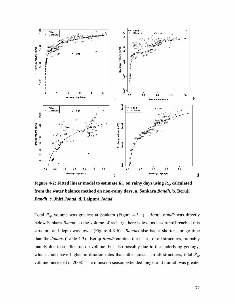
72
a b
c d
Figure 4-2: Fitted linear model to estimate Rep on rainy days using Rep calculated
from the water balance method on non-rainy days, a. Sankara Bandh, b. Beruji
Bandh, c. Jhiri Johad, d. Lalpura Johad
Total Rep volume was greatest at Sankara (Figure 4-3 a). Beruji Bandh was directly
below Sankara Bandh, so the volume of recharge here is less, as less runoff reached this
structure and depth was lower (Figure 4-3 b). Bandhs also had a shorter storage time
than the Johads (Table 4-3). Beruji Bandh emptied the fastest of all structures, probably
mainly due to smaller run-on volume, but also possibly due to the underlying geology,
which could have higher infiltration rates than other areas. In all structures, total Rep
volume increased in 2008. The monsoon season extended longer and rainfall was greater

73
in 2008, which is reflected in the Rep volume with a longer time series and greater volume
than in 2007 (Figure 4-3).
a b
c d
Figure 4-3: Estimated Rep (m3) with daily rainfall (mm) from Bhaonta gauge for
a. Sankara Bandh, b. Beruji Bandh, and with daily rainfall from Hamirpur gauge
for c. Jhiri Johad, d. Lalpura Johad
There is greater daily Rep (mm) with greater storage depth in the structures, than with less
stored water (Figure 4-4). For the two Bandhs (Figure 4-4 a and b) there is an
approximately linear increase of daily Rep (mm) with increasing storage depth. Lalpura
Johad also indicates an increase in daily Rep (mm) with greater depths, but the

74
relationship might be more non-linear. The slopes of the fitted linear models in Figure 4-
4 are similar for all structures, but lowest in Sankara Bandh, which is a reflection of the
size of the structure. At Sankara Bandh, for each incremental increase in depth, a larger
surface area of water is required compared to the other smaller structures, which have
higher daily Rep response with increasing depth, but smaller Rep volume.
a b
c
Figure 4-4: Average Depth (mm) by daily Rep (mm) for a. Sankara Bandh, b. Beruji
Bandh, c. Lalpura Johad, (where Rep (mm) is calculated by dividing Rep (m3) by
average surface area (m2))
An analysis of variance model was fitted for recharge by site, then structure and finally
recharge by structure type, which were all significant variates. Due to the higher rainfall

75
in 2008, the RWH structures stored a greater volume of water, so that by site, structure
and structure type, the statistical analysis indicated differences in the results between the
two monitored years (Table 4-2). Using Tukey HSD, there were no significant
differences between focus areas in 2007, whereas in 2008 Jhiri Johad was significantly
different from the others. Bandhs and Johads are significantly different in 2008, but not
in 2007. This is most probably due to higher average rainfall in 2008, which meant that
the larger structures, the Bandhs, could store more water than the Johads and thus Rep
increased. The rainfall at Sankara Bandh (Bhaonta gauge) had the lowest rainfall in
2007, yet Sankara Bandh held the highest storage. This is due to the catchment area of
this structure, which is larger than all the other monitored structures and is located in the
steep rocky hills.
Differences in Rep are difficult to interpret, given the variability in Rep volume, which
depends on the shape and size of structure storage, runoff characteristics (local rainfall
and land cover), and infiltration characteristics in the storage area (soil depth and
underlying bed rock), but these differences indicate the local variability. In the Johads,
the soil depth was deeper and had higher clay content compared to Bandhs, which would
influence the infiltration capacity of the stored water to reach the groundwater
(Table 3-9).
Table 4-2: Tukey HSD results of potential recharge by focus area and RWH type
Significant Difference by: 2007 2008 Both Years
Focus area
(Bhaonta, Lalpura, Jhiri)No
Yes, except
Lalpura – Bhaonta
Yes, except
Lalpura – Bhaonta
RWH structure type
(Bandh, Johad)No Yes Yes
As rainfall increases, the volume of Rep increases. Compared to 2007, in 2008 the total
volume of Rep at Sankara Bandh increased 3 times, Beruji Bandh 2.3, Jhiri Johad 2.0 and
Lalpura Johad 2.1 times. As only two years of field data has been collected, it is difficult
to determine the exact relationship between annual rainfall and annual recharge. The

76
observed data however, indicate the range of Rep values that can occur across a variable
landscape. Such variability can be included in models via Monte Carlo simulations or
can assist with parameter estimation.
The average daily Rep rates (Table 4-3) in 2008 are much greater than in 2007, as more
rainfall in 2008 meant more stored water in the RWH storage areas and therefore more
Rep. Studies conducted on recharge through percolation tanks constructed in hard rock
and alluvium formations in the Pali district (Western Rajasthan), showed similar
percolation rates of 14 – 52 mm/day (Narain, Khan et al. 2005). Another study by
Neumann et al. (2004) theoretically compared evaporation rates with different recharge
rates from structures. They found that rates varied broadly for different reservoirs.
Decline rates that were similar to evaporation rates (3.6 mm/day) suggested that
reservoirs were 100% inefficient, acting only as evaporation pans. Other reservoirs with
decline rates of 24 mm/day or greater suggested more recharge, which is similar to all
monitored RWH structures in this study (Table 4-3). Neumann et al. (2004) points out
that the rate of infiltration from structures can change throughout the season due to:
change in hydraulic gradient, the shape of the storage area and runoff into the structure,
carrying with it sediments which build up over time forming a layer.
Table 4-3: Average daily Rep (mm/day) and number of days water stored in
monitored RWH structures in 2007 and 2008
RWH Structure YearTotal days
of storage
Average daily
Rep (mm/day)
Standard deviation
of Rep
Sankara Bandh2007 169 45.6 0.07
2008 206 55.6 0.15
Beruji Bandh2007 138 20.9 0.07
2008 201 27.8 0.03
Jhiri Johad2007 273 12.3 0.01
2008 308 19.5 0.01
Lalpura Johad2007 240 15.7 0.02
2008 382 23.5 0.04

77
4.2.2.2. Potential Recharge and Rainfall Relationship
As explained, rainfall in this study area is highly localised. This must be considered
when examining the relationship between rainfall and potential recharge, because those
structures that were closest to a rain gauge may have stronger relationships. At Sankara
Bandh and Beruji Bandh, the rainfall gauge was approximately 2 km from the structures.
However the nearest rain gauge for Lalpura Johad was 8.5 km away, and for Jhiri Johad
2.5 km.
The exponential function, as used by Sharda et al. (2006), was fitted to cumulative sum of
rainfall and cumulative sum of Rep over the two year time series:
10log ( ) [ ]cPepR a b e
Eq 4-5
epR = cumulative recharge (mm), P = cumulative rainfall (mm), a, b and c = parameters
This function gives estimates of cumulative recharge from cumulative rainfall, which is
useful to identify how much rainfall would be needed for a given amount of Rep.
Potential recharge was converted from m3/day to mm/day by dividing by the average
surface area of the structures (See Section 4.2.1.1).
Logarithmic and logistic sigmoid curves were also fitted, but the exponential function
(Eq 4-5) had the best fit, with high R2 (Table 4-4). In all structures, Rep from RWH
reaches a maximum daily depth as cumulative rainfall continues to infinity, a relationship
also described in Sharda et al. (2006) (Figure 4-5). This reflects the engineering design
of the structures, which can only store a limited amount of runoff, regardless of how
much rainfall and so can only induce a maximum depth of daily recharge.

78
Table 4-4: Statistical parameters for Eq 4-5 describing the relationship between the
cumulative sum of Rep (mm) and cumulative sum of rainfall (mm)
Structure R2 a b c
Sankara Bandh 0.89 2.78 1.94 0.004
Beruji Bandh 0.88 2.86 0.21 0.005
Jhiri Johad 0.93 2.78 0.75 0.003
Lalpura Johad 0.81 2.68 0.77 0.008
In Sankara Bandh (Figure 4-5 a) two distinct trends can be seen, which reflects the
different rainfall patterns of 2007 and 2008. The intensity of rainfall in 2007 was smaller
than in 2008 (Figure 4-6). This resulted in the higher cumulative recharge daily depth
that is seen at Sankara Bandh. Jhiri Johad also displays this pattern, but 2007 cumulative
Rep depth is higher than the 2008 cumulative Rep (Figure 4-5 b). This is more difficult to
explain, but could be associated with a different rainfall pattern in this location, with
perhaps a large rainfall event early in 2007. Beruji Bandh does not display this
difference, because it is situated below Sankara Bandh storage, so runoff from a large
rainfall event takes more time to reach this structure (Figure 4-5 c). Lalpura Johad
similarly displays the lack of response to higher rainfall events (Figure 4-5 d). The steps
in the data in Figure 4-5 is because recharge is continuous, while rainfall does not occur
each day.

79
a b
c d
Figure 4-5: Cumulative potential recharge (mm) against cumulative rainfall (mm)
using the exponential function (y axis is logged) a. Sankara Bandh,
b. Beruji Bandh, c. Jhiri Johad, d. Lalpura Johad

80
Figure 4-6: Cumulative rainfall for 2007 (mm) against cumulative rainfall for 2008
(mm) (line represents x = y)
Figure 4-7 displays the cumulative rainfall required to induce 1 mm, 10 mm and 100 mm
of Rep from the monitored RWH structures, calculated from the regressions in Table 4-4
and Eq 4-5, and are comparable with the results in Sharda et al. (2006). This is a positive
result, because the data collected from the Sharda et al. (2006) study was across a smaller
area and contained less noise than this study. Beruji Bandh, Jhiri Johad and Lalpura
Johad display very similar results to the Sharda et al. (2006) estimates. However Sankara
Bandh requires less cumulative rainfall to induce recharge. This may be because Sankara
Bandh has a larger storage, and is situated in the steep rocky hills, where percolation is
highest (Table 4-3). Beruji Bandh requires more cumulative rainfall to induce recharge,
which is a reflection of the position of Beruji Bandh, below Sankara Bandh (which would
first collect runoff), and in a smaller catchment area. The Johads, Lalpura and Jhiri, hold
water in storage for the longest time (Table 4-3), due to lower infiltration rates in the
storage areas. More rainfall is needed for these structures to induce more Rep. These
results highlight the difference in Rep between the larger and smaller RWH structures.

81
Figure 4-7: Cumulative rainfall (mm) required for 1 mm, 10 mm and 100 mm of Rep
for each monitored RWH structure and compared with estimates from Sharda et al.
(2006)
4.2.2.3. Recharge Efficiency of RWH Structures
Despite the uncertainties associated with the field measurements of RWH surface area
and depth, stored run-on volume into each monitored RWH structure was estimated to
determine the recharge efficiency. Given these uncertainties, there is a not a large
difference between years in these results (Table 4-5). In 2007 the volume stored in the
structures was much less than in 2008, but this does not seem to influence recharge
efficiency, as the volume of run-on is in a similar ratio to Rep volume across the two
years.
The most efficient RWH structure is Beruji Bandh. More of the water stored in this
structure became potential recharge than in any other structure, which could be because it
had the shortest storage time and therefore less evaporative losses (Table 4-3). In 2008

82
there is a greater storage surface area in all the RWH structures, but shallower depths at
the exteriors of the storage area. A larger surface area therefore means greater
evaporation losses, as the high surface area to volume ratio of small reservoirs leads to
higher evaporation loss (Keller, Sakthivadivel et al. 2000). This is possibly why Sankara
Bandh, with the highest potential recharge volume, but also the largest storage surface
area (and therefore higher evaporative losses), has lower recharge efficiency than Beruji
Bandh.
Johads have similar recharge efficiency. The Johads at Jhiri and Lalpura held water in
storage longer than in the Bandhs, and so evaporative losses would have been higher
(Table 4-3). As described in Table 3-9, the deeper heavier clay layer in these structures,
and underlying geology, mean that infiltration rates are smaller in Johads, so hold stored
water for longer. These structures are known in the community to not have a large
recharge component, which was confirmed in this study, and are purpose built to store
water for cattle bathing and drinking.
Table 4-5: Recharge efficiency of RWH structures in 2007 and 2008
RWH structureRecharge efficiency %
2007 2008
Sankara Bandh 6.0 8.2
Beruji Bandh 16.4 14.1
Jhiri Johad 2.1 1.3
Lalpura Johad 3.4 4.1
4.2.3. River flow and Storage
In much of the literature that considers RWH impacts, the upstream-downstream trade
offs are often highlighted as a potential problem, but this has never been quantified.
These trade offs were also considered when conducting field work in the case study, and
discharge across three Anicuts that lie across the main reach of the river were monitored.

83
As already highlighted, there is a large variability in rainfall, which is reflected in the
overflow from the Anicuts on the river. In 2007, the Anicut at Hamirpur overflowed on 8
days towards Kaled. At Kaled Anicut, overflow occurred for 22 days and further
downstream towards Sainthal Sagar dam, at Sirinagar, there was no river flow (refer to
Figure 3-1 for catchment position). On the other tributary, at Nitata, the Anicut
overflowed on 6 days. In 2008, rainfall increase led to more overflow; Hamirpur 24
days, Nitata 11 days, but Kaled had the longest overflow, flowing daily through the
months of July to early November (Figure 4-8).
Figure 4-8: Daily discharge or overflow over the monitored Anicuts on the Arvari
River in 2007 and 2008
Discharge and days of overflow was greatest at the Kaled Anicut in both years
(Figure 4-8). Either more rain fell in the catchment of the Kaled Anicut, or perhaps the
larger Anicut at Samra, which is above Kaled Anicut and below Hamirpur Anicut,
released water slowly downstream. The latter reason seems more likely because in 2008
flow occurred daily from July until November (there was no rain after September in
2008). The peaks in all the Anicuts fall at similar times, mostly when large rainfall events
occurred and therefore there were greater runoff events into the river.

84
At Hamirpur Anicut, overflow started at a similar cumulative rainfall in both years
(Figure 4-9 a). At Kaled and Nitata Anicuts the cumulative overflow from the structures
was much greater in 2007 than for a similar cumulative amount of rainfall in 2008
(Figure 4-10 b and c). Due to the high variability of rainfall, the use of the same rainfall
at Kaled and Nitata as Hamirpur may produce these results. However, it could also
possibly suggest that more water reached the stream earlier in 2007 than in 2008 at these
locations. Perhaps more water was captured upstream in 2008 than in 2007. In 2008
there were larger rainfall events, which RWH is most efficient in capturing. While this
study can not compare the impact of RWH on streamflow before and after RWH works
began, this analysis suggests that the rainfall – stream runoff relationship may have been
altered. In 2008, even though 300 mm rain fell in a much shorter time period than in
2007 (Figure 4-6) due to the difference between the smaller number of rainfall events in
2007 and the larger number of rainfall events in 2008, the streamflow is not as great.
This suggests that RWH may be capturing runoff in larger events, which would otherwise
reach the river. This analysis also indicates that for overflow at the Anicuts to occur,
concurrent events of rainfall is just as important as the cumulative amount of rainfall.

85
a b
c
Figure 4-9: Cumulative sum of rainfall (mm) at Hamirpur against cumulative sum
of overflow on the Anicuts on the Arvari River at a. Hamirpur, b. Kaled, c. Nitata
Given that no surface areas were measured for the water stored in the Anicuts, the depth
of recharge from the Anicuts was estimated using the water balance method for days
when there was no overflow, no rainfall and no runoff in the storage.
epR h ET Eq 4-6
h = change in depth behind dam wall, ET = potential evaporation.
This assumes that Rep occurs evenly over the storage surface area. As a result the actual
total Rep volumes would differ from these estimates, as these would be related to the
surface area.

86
Figure 4-10 shows the differences in recharge at the Anicuts. Average daily recharge
varied from 42 mm/day at Nitata, to 25 mm/day Kaled and 44 mm/day at Hamirpur.
Kaled was the smallest structure, with the lowest dam wall height, which could be why
Rep was lowest here. Interestingly in all Anicuts recharge appears higher in the low
rainfall year (2007). In 2008 there was more overflow (Figure 4-8), so there was not a
long enough time series to establish Rep. Potential recharge could only be estimated once
overflow had stopped and so actual Rep could be much higher. This could explain the
lower values at Kaled Anicut. But overall these estimated Rep values are high when
compared with the values obtained from the Johads and Bandhs, possibly due to
differences in underlying stratum. This confirms the notion that the structures on the
river are important for recharge. These results could also provide approximate
transmissions losses from the river reaches.
Figure 4-10: Estimated Rep (mm/day) from monitored Anicuts on the Arvari River
in 2007 and 2008
After the first few rainfall events, it was observed that water accumulated downstream of
all three Anicuts on the river. This water was not flowing, and it was assumed either to

87
be leakage from the dams or upwelling base flow from the shallow alluvial aquifer. This
water was present from July 2007 to early 2008, and again in the monsoon of 2008 to
early 2009. Based on EC measurements, it appears that the water is not base flow but
lateral subsurface flow from the water stored in the Anicut upstream (Figure 4-11). The
EC values of the water downstream of the Anicuts are closer to the EC values of water in
the storage of the Anicuts than to values in the groundwater in the nearby monitored dug
wells. From this data, there is also seen an increase in salinity levels in groundwater as
water levels decline. This could be from return flow from irrigated agriculture, which
increases salinity in the groundwater.
a b
c
Figure 4-11: Measured EC (mS/cm-1) values in Anicuts and dug wells in 2008 in the
focus areas of a. Kaled , b. Nitata, c. Hamirpur

88
Conclusions
Some general characteristics of RWH structures can be determined from the above
analysis, despite uncertainties associated with the field data. In all RWH structures the
higher than average rainfall in 2008, increased the total volume of Rep and average daily
Rep depth. But recharge efficiency was similar between years and structures, which
suggest that the efficiency of RWH is a function of location, size and shape rather than
amount of rainfall received. This also limits the maximum daily recharge depth of the
structure, which would also be related to the saturated hydraulic conductivity of the
underlying stratum. Nevertheless high rainfall years influence the amount of runoff and
therefore the volume of Rep from a RWH structure.
4.3. Well Data Analysis
4.3.1. Recharge Estimate in Wells – Water Table
Fluctuation (WTF) Method
The water table fluctuation (WTF) method is used to estimate recharge from the
monitored dug well data. It requires knowledge of the specific yield (Sy) and change in
groundwater levels over time (Healy and Cook 2002). The amount of recharge
( gwR mm/day) can be estimated from the rise in the water table ( h ) over time ( t )
(Healy and Cook 2002; Scanlon, Healy et al. 2002):
.gw yR S h t Eq 4-7
A constant specific yield (Sy) was taken as 0.1, based on literature data (Table 4-6),
assuming an unconsolidated geological formation. The lithology of the area is
predominantly alluvium and blown sand (Table 4-7), which, according to standard Sy
values (Johnson 1967), would give a similar estimate. Furthermore in the Banganga
River Basin, of which the Arvari River catchment is a part, Sy in alluvial aquifers ranges
from 0.07 – 0.15 (Ground Water Department Jodhpur 1999). While assuming a constant

89
Sy can introduce errors in the recharge estimations (Sophocleous 1991), there is little
other data to allow a more accurate estimation of Sy, such as used in other studies
(Crosbie, Binning et al. 2005; Marechal, Dewandel et al. 2006; Muralidharan and
Andrade 2007; Wendland, Barreto et al. 2007).
Table 4-6: Generalised aquifer characteristics for aquifers across India and most
likely occurring in the Arvari River Catchment (COMMAN 2005a)
Geological formation Sy % T m2/day
Unconsolidated 5-18 250-4000
Semi-consolidated 1-8 100-2300
Table 4-7: Description of geology in areas where monitored dug wells
VillageNumber of
monitored dug wells
Lithology (Geological Survey of
India 1999)
Bhaonta 6Intertrappean quartzite,
conglomerate
Lalpura 2 Alluvium and blown sand
Jhiri-Lalpura road 3 Alluvium and blown sand
Jhiri 1 Alluvium and blown sand
Hamirpur-Kaled road 5 Schist and alluvium
Hamirpur 4 Intertrappean schist
Kaled 6 Alluvium and blown sand
Nitata 2 Alluvium and blown sand
4.3.2. Results
4.3.2.1. Well Response
Water levels in all monitored wells increased during the monsoon seasons in 2007 and
2008. The rate of increase is different for each well, which could be due to a range of

90
factors including: aquifer properties, number of RWH structures nearby, and the amount
and intensity of rainfall in the local area. While this variability means that strong
conclusions are difficult, it highlights local catchment variability, a common feature of
semi-arid areas (Pilgrim, Chapman et al. 1988) and also the local recharge impacts of
RWH.
Most wells had diesel pumps and these were used extensively for irrigation during the
monsoon of 2007 due to the low rainfall. Consequently water levels in pumped wells
decreased significantly after reaching a maximum height early in the monsoon of 2007
(which may not actually have been the maximum groundwater level because of pumping
effects). This made it difficult to estimate recharge using the water table fluctuation
(WTF) method. On the other hand the rainfall in 2008 was mostly sufficient for meeting
Kharif crop needs, resulting in less pumping, especially in the early months of the
monsoon (July – August), so the water level rises in the wells can be seen more clearly in
2008 and reached a higher level.
Data from all monitored wells, including those close to the monitored Bandhs and
Johads, those close to monitored Anicuts on the rivers, and wells not close to a RWH
structure, is reported. In the accompanying figures, water levels are plotted as heights
above sea level (ASL) and also as relative groundwater levels, where relative height is
defined as:
int
max
( )
( )inital
t ialh hrelative height
h h
Eq 4-8
ht = height ASL (m) at time t, hinitial = initial groundwater level height ASL (m), hmax =
maximum groundwater level height (m)
Using relative groundwater level heights allows easier comparison of the recharge
behaviour (or rise) in wells in similar areas, and is particularly useful to examine whether
any of the wells recharge faster than others.

91
a b
c
Figure 4-12: The six monitored wells at focus area Bhaonta, a. ASL (m)
groundwater level, b. Relative groundwater level height, c. Relative groundwater
level height at Well BK5 and depths at Sankara Bandh and Beruji Bandh (m)
The wells at Bhaonta saw a greater response in 2008 than 2007 (Figure 4-12 a and b).
There was less pumping and more rainfall, so the impact of recharge can be seen more
clearly. Wells BK1 and BK2 were closest to the two large Bandhs, but were pumped in
2007. The relative response in 2008 shows a greater increase in these wells compared
with BK3 and BK6 (Figure 4-12 b). In general, wells BK1, BK2, BK4 and BK5 show
faster responses than BK3 and BK6. This could be due to their position in the landscape.
Wells BK3 and BK6 are in a valley that runs parallel to the valley with the Bandhs, so

92
recharge may take longer to reach there due to different geology (Appendix 1). Well
BK4 is further away from the structures than well BK3, and aquifer connectivity
probably has some influence on the difference in response between these two wells. Well
BK5 was the shallowest well, close to the surface in a rocky area, while BK1 and BK2
were in the agriculture land. The response from well BK5 closely mirrored the RWH
structures water storage patterns of rise and fall (Figure 4-12 c.), which confirms the
influence of recharge from RWH on groundwater levels. Wells BK4 and BK 6 are
almost 1 km away from Sankara Bandh and 600 m from Beruji Bandh, but the influence
of recharge on groundwater levels can still be clearly seen. This could be the result of
large lateral transmissivity as Bhaonta is in the rockier higher elevation area and there are
larger volumes of potential recharge coming from the Bandhs, particularly from Sankara
Bandh (Figure 4-3).
a b
Figure 4-13: The two monitored dug wells at focus area Lalpura, a. ASL (m)
groundwater level, b. Relative groundwater level height (m)
The two wells below the Lalpura Johad had diesel pumps, which were used in both 2007
and 2008 (Figure 4-13). This makes it difficult to determine any recharge trends.
Nevertheless well LP1 is situated directly in front of the Lalpura Johad and the relative
response from this well was greater than at well LP2, which is further away. This
suggests that recharge from Lalpura Johad has a smaller mounding influence on the

93
water table because it does not effect dug wells further away, whereas at Bhaonta, rises
were seen in wells 6 km away. Alternatively the aquifer connectivity may be poor, with
lower transmissivity, but the Lalpura focus area is in a similar landscape position and
elevation to Bhaonta, so the former conclusion may be more apt.
Figure 4-14: The monitored well at Jhiri ASL groundwater level (m)
There was only one well close to the Jhiri Johad structure, which was also pumped
(Figure 4-14). The response is greater in 2008 than in 2007 which could be due to less
pumping and/or more recharge.

94
a b
Figure 4-15: The four monitored dug wells at Hamirpur a. Groundwater level ASL
(m), b. Relative groundwater level height (m)
In Hamirpur all wells, which were close to the monitored Anicut on the river, similarly
showed a greater relative response in 2008 than in 2007 (Figure 4-15). There was much
less pumping from all wells in 2008. Wells HP2 and HP3 are directly next to each other
and consequently are very similar. Wells HP1 and HP4 are closest to the river, while
well HP1 is closest to the Anicut. However the response from these wells is very similar
to HP2 and HP3 which are further away (Figure 4-15 b). This might indicate a fast
lateral transmissivity in this area.

95
a b
c
Figure 4-16: Response of monitored wells at Kaled a. Groundwater level ASL (m),
b. Relative groundwater level height (m), c. Relative groundwater level height (m)
well KLD6
At Kaled, wells KLD1 – KLD5 are all along the river below the Anicut and display
similar characteristics in response (Figure 4-16 a and b). Well KLD6 is more than 1 km
away from the river and as a result the response here was slower and perhaps does not
reflect the mounding influence of the Anicut nearby, but the overall recharge in the
aquifer (Figure 4-16 c). Well KLD6 also indicates a higher response in 2008 than 2007.
There was no pump on this well, so rise here is related to recharge reaching the aquifer in
this area. This indicates that overall recharge was much higher in 2008 compared to
2007.

96
a b
Figure 4-17: Response of two monitored dug wells at Nitata, a. Groundwater level
ASL (m), b. Relative groundwater level height (m)
The two wells near the Anicut at Nitata follow each other in response (Figure 4-17). Well
NT1 is above the Anicut, while well NT2 is downstream from the Anicut. Water stored in
the structure percolates into the aquifer, influencing both wells. Alternatively, well NT1
might be influenced by transmission losses from water flowing into the Anicut storage
area.
a b
Figure 4-18: Roadside wells between Jhiri and Kaled. a. Groundwater level ASL
(m), b. Relative water level height (m)

97
The roadside wells in Figure 4-18 are situated between the Jhiri and Kaled focus areas.
These wells were not situated as close to RWH structures as the other wells and as such
could be interpreted as background values of recharge. Water levels in well RD3
continue to rise when other wells nearby have already decreased (Figure 4-18 a). This
well was in the valleys, not close to a RWH structure or the river, and was not pumped.
The slow response of this well most likely represents lateral flow in the shallow alluvial
aquifer, by transmission through the aquifer, rather than natural recharge in the area of
the well itself.
Further monitored roadside wells are between Jhiri and Lalpura in the upper catchment
(Figure 4-19). The wells on the roads still reflect increasing recharge in 2008, though the
rate of increase is not as high as those wells close to RWH structures.
a b
Figure 4-19: Monitored dug wells along roadside from Jhiri to Lalpura
a. Groundwater level ASL (m), b. Relative water level height (m)

98
4.3.2.2. Trends of Well Recharge in the Monitored
Area
Figure 4-20 and Figure 4-21 show groundwater levels ASL (m) in the dug wells that have
been interpolated across the surrounding area using the Inverse Distance Weighting
method. This is mainly to show general trends and is not a rigorous spatial analysis.
Figure 4-20 a and Figure 4-21 a are pre-monsoon levels (1st June) in 2007 and 2008
respectively, Figure 4-20 b and Figure 4-21 b are towards the end of the monsoon (12th
September) for each monitored year. The interpolation was done within the area of the
monitored wells, rather than extrapolating to the whole spatial area in the catchment
(Figure 3-6). The pre-monsoon maps look very similar between years, which would be
expected as local management practices results in water levels being pumped to a similar
depth each year. The post-monsoon levels are higher in 2008 (Figure 4-22 b) than in
2007 (Figure 4-21 b), which reflects the greater amount of both rainfall and recharge
from RWH structures in 2008 and less pumping. The maps also clearly indicate spatial
variability in recharge and a general slope of the watertable towards the south east.

99
a b
Figure 4-20: Inverse Distance Weighted Interpolation of monitored well heights
ASL (m) a. 1st June 2007, b. 12 September 2007
a b
Figure 4-21: Inverse Distance Weighted Interpolation of monitored well heights
ASL (m) a. 1st June 2008, b. 12 September 2008

100
4.3.3. Recharge Estimates in the Groundwater Table
(Rgw) – Water Table Fluctuation Method
A daily time step was used to calculate Rgw using the water table fluctuation (WTF)
method with a constant Sy of 0.1 for all monitored wells. The most unaffected section of
the time series was used to estimate Rgw. In 2007, due to heavy pumping, the unaffected
time series for each well was very short, and for some wells not available. In 2008
however, the unaffected sections of the time series were longer as there was less
pumping. The WTF method was applied mainly to the rise in dug well at the start of the
monsoon season in both years. Also analysis of this section of the time series coincides
with the steeper part of the groundwater rises, which means it is likely to result in more
accurate estimates of recharge, because it would be less affected by lateral transmission
than the latter part of the series. Not all negative change in depth is due to direct
pumping. Some wells that are not pumped decrease in depth during the monsoon season,
which could be due to pumping influence from wells nearby.
a b
Figure 4-22: Interpolation of average Rgw (mm/day) from WTF method in
a. 2007, b.2008

101
Average Rgw (mm/day) was estimated for each dug well monitored in each year. Due to
the lack of information about the extent and properties of the local aquifer, it is difficult
to extrapolate this to a volumetric increase in the aquifer. The average daily Rgw rates
(mm/day) for each year were spatially interpolated using the Inverse Distance Weighting
method (Figure 4-22).
The average daily Rgw rates (mm/day) were higher in 2008 than 2007 (Figure 4-22).
Despite the uncertainty of interpolation, the general trends that can be seen show that
moving down the catchment, and to lower elevations, estimated daily Rgw increases. This
might suggest flow of groundwater down the catchment is dictated by elevation.
However the wells at Hamirpur and the wells south of the focus area of Hamirpur, have
higher recharge rates than at Kaled and Nitata focus areas, which are further downstream
(Table 4-8). This may be due to the position in the landscape. If groundwater is moving
towards lower elevations, Hamirpur and the surrounds are at slightly lower elevations
than Nitata and Kaled (Figure 4-23). Another interpretation is that the aquifer properties
in these areas are different, and the WTF method in this study assumes a constant Sy
throughout the catchment. It might be possible to deduce the lateral movements from the
temporal variation in well responses down the catchment. However due to spatial and
temporal distribution of rainfall such an analysis is not straight forward.

102
Figure 4-23: Digital Elevation Model (DEM) for the area of the monitored dug wells
Table 4-8: Average Rgw (mm/day) in the focus areas in the Arvari River catchment
using the WTF method
Focus AreasNumber of
monitored wells
Average Rgw
(mm/day) 2007
Average Rgw
(mm/day) 2008
Bhaonta 6 4.6 7.2
Lalpura 2 2.5 7.5
Jhiri-Lalpura road 3 4.1 6.9
Jhiri 1 NA 7.3
Hamirpur 4 12.4 23.9
Jhiri- Kaled road 5 9.6 13.1
Kaled 6 7.3 13.0
Nitata 2 10.0 11.5

103
4.4. Summary and General Discussion
4.4.1. Comparison of Recharge Estimates
The average daily potential recharge (Rep mm/day) from the monitored RWH structures
was greater in 2008 than in 2007 and this increase was also seen in the water table
response in the wells (Rgw mm/day). However average daily Rep is much greater than
average daily Rgw for wells close to the structures (Figure 4-24). This difference could be
either due to a large amount of lateral flow or due to water stored in the soil profile below
the RWH storage area. This is further examined by estimating hydraulic properties of the
soils in the RWH storage areas. Based on the field textures (Table 3-9) and using the soil
texture triangle (Saxton, Rawls et al. 1986), field capacity (FC), available water (AW) and
saturated hydraulic conductivity (Ksat) of the soil in RWH storages is obtained (Table 4-
9). Using these characteristics, approximately 30% of Rep is held in the soil, and about 13
– 32% is Rgw (Table 4-10). Approximately 30 – 50% of the difference could be lateral
flow, as groundwater moving down the catchment. Sankara Bandh was furthest away
from the wells in a hillier area, so a larger lateral flow component is more expected
(Table 4-10). Larger local mounds, such as possibly under Sankara Bandh, would also
increase hydraulic gradients and thus increase lateral movement of water. There is
possibly less lateral flow from the Johads, Jhiri and Lalpura, due to higher storage in the
soil and lower recharge values.

104
Figure 4-24: Comparison of Rep estimates from monitored RWH (mm/day) and Rgw
in monitored dug wells (mm/day) in 2007 and 2008
Table 4-9: Hydraulic properties for soil in monitored RWH structures using the soil
texture triangle (cm3 water/cm3 soil) (Saxton, Rawls et al. 1986)
Structure Soil texture % Sand % Clay FC AW Ksat (cm/hr)
Sankara Bandh Silt Loam 20 20 0.29 0.17 0.48
Beruji Bandh Silt Loam 20 20 0.29 0.17 0.48
Jhiri JohadSandy Clay
Loam50 30 0.28 0.11 0.29
Lalpura Johad Sandy Clay 50 40 0.32 0.10 0.15
The high lateral flow potential also suggests that the rise in groundwater table in wells
not close to RWH structures is more likely to be recharge from RWH structures than
natural recharge. Natural recharge estimates from the regression developed by
Rangarajan et al. (2000) for alluvial areas gives approximately 57 mm/year of natural
recharge in 2007 and 104 mm/year of natural recharge in 2008 in the Arvari River

105
catchment. These estimates are smaller than actual rise in groundwater, which range
from approximately 200 – 300 mm in the monsoon season.
Table 4-10: Example analysis of movement of Rep through the soil profile on one day
in 2008 (mm/day)
Structure
Average
Rep
(mm/day)
FC
%
Rep as
soil water
(mm/day)
Rep – soil
water
(mm/day)
Rgw
(mm/day)
Average
lateral
flow
(mm/day)
lateral
flow %
Sankara
Bandh55.6 29 16.1 39.5 7.2 32.3 58
Beruji
Bandh27.8 29 8.0 19.7 7.2 12.5 45
Jhiri
Johad19.5 28 5.5 14.0 7.3 6.7 35
Lalpura
Johad23.5 32 7.5 16.0 7.5 8.5 36
4.4.2. Potential Recharge from RWH in the Catchment
Based on data from the NGO, Tarun Bharat Sangh, the storage area of RWH structures is
about 1.44% of the Arvari River catchment area, which is an underestimate but was used
as the tested RWH density in this study. The RWH storage surface area was considered
to be the same for 2007 and 2008 for the calculation presented in Table 4-11. This is
erroneous because in 2008 there was more rainfall, which increased the storage surface
area, but this study can not confirm by how much. The rainfall at Hamirpur was used to
calculate the percentage of rainfall that becomes recharge from Anicuts/Bandhs and
Johads/Talab in the catchment (Table 4-11). These structures were grouped because of
similarities in size.

106
In 2007 around 6.6% of rainfall became Rep, and in 2008 about 7% of rainfall became Rep.
These values are actually quite similar to the recharge efficiency estimates from the
monitored RWH structures (Table 4-5). The fraction of rainfall that becomes recharge is
also very similar between a dry and a wet year, which reflects the recharge efficiency of
the structures.
Table 4-11: Approximate area of the catchment for different RWH structure types
in the Arvari River catchment and approximate percentage of annual rainfall that
becomes Rep in 2007 and 2008
Structure % Area of
Catchment
% Annual Rainfall
2007 2008
Anicut/Bandh 0.82 9.5 9.1
Johad/Talab 0.61 2.4 4.0
Total 1.44 6.6 7.1
4.4.3. Discussion and Conclusions
In a data sparse environment such as this area, first estimates of catchment characteristics
such as recharge, flow in the river and climatic patterns are an important step towards
understanding the existing hydrological processes in the catchment. This is particularly
relevant for management actions that could impact catchment hydrology, including
rainwater harvesting. The main outcome of this chapter is the field data from the Arvari
River catchment collected in 2007 and 2008 indicating large variability in space and time.
There were significant limitations to the field data collection in the catchment. For the
catchment community, measuring wells and stored water in RWH structures was a
novelty, as the collected field data is the first of its kind for this area. The Arvari River
catchment has very little infrastructure, with subsistence farming the main livelihood
(Chapter 3). Consequently the facilities and infrastructure in the area are quite poor and
this limited the field data collection. Roads were sometimes inaccessible and in disrepair.
Climate and weather also constrained the ability to do field work with extreme

107
temperatures and intense rainfall at times. Additionally, measurements of the surface
areas of stored water in RWH structures were often difficult due to inaccessibility.
Nevertheless the main aim of the field work was to obtain, relatively rapidly, a large
number of data points over an inhomogeneous catchment area. In the end, the overall
number of observations is modest and techniques used basic and so there are
measurement uncertainties. However this chapter indicates that despite these
shortcomings, it was still possible to develop a relatively accurate picture of local-scale
water balances and catchment-scale variability.
The focus areas were in the upper and middle reaches of the catchment. In this relatively
small area, rainfall exhibited a highly variable temporal and spatial pattern, with localised
events (Section 3.2.2). The 2007 season had below average annual rainfall while 2008
had above average annual rainfall. Within each year event size and distribution was very
variable. This is typical of monsoonal rainfall in Rajasthan where rainfall is characterised
by short intensity, localised and variable within a basin (Sharma and Murthy 1995).
The method used by Sharda et al. (2006) to estimate recharge from RWH structures was
used here to analyse the data collected from the RWH structures, and results generally
agree with their findings and of Badiger et al. (2002), that less than 10% of rainfall
becomes potential recharge. However higher potential recharge was observed locally
which would explain observations by Muralidharan and Andrade (2007). While the
results are limited by the length of the time series available, this study compares a
comparatively wet and dry year and this indicates variation in possible recharge. The
impact of higher annual rainfall on recharge can be clearly seen in 2008, with higher
rainfall resulting in more overall potential recharge. Despite this variation in rainfall the
fraction of rainfall that becomes recharge was very similar between the years. Potential
recharge from the structures reaches a limiting point with increasing rainfall, which is a
factor of the maximum storage capacity in the structure. However, a difference in Rep
was found between Bandhs and Johads, with an average Rep of 37.5 mm/day for Bandhs,
and 17.8 mm/day for Johads. This may be related to the fact the observed Bandhs were
located on more porous material and thus highlights the importance of careful positioning

108
of the structures. Interestingly while Rep amounts were higher in 2008, recharge
efficiencies were about the same for the two years. Efficiency is a function of infiltration
and structure shape and size rather than rainfall amount. These factors also influenced
the amount of rainfall that becomes recharge. For any attempt to model RWH in the
catchment, it would be recommended to calibrate the model so that a similar percentage
of rainfall becomes potential recharge as found in this chapter.
The analysis of the well data was difficult because of the amount of pumping, particularly
in 2007. But by taking the most unaffected sections of the time series, and assuming a
constant specific yield, estimates of Rgw ranged from 7.2 mm/day to 11.3 mm/day.
Recharge estimates increased moving down the catchment in elevation. The recharge
values from the wells were much lower than the estimates of potential recharge from the
RWH structures. This suggests that either the recharge from RWH is not reaching the
aquifer, or the aquifer has large transmissivity and therefore strong lateral flow. The
analysis in this chapter suggests that about 30% Rep is stored in the soil while at least
another 30% moves laterally. As a result the water recharged becomes spreads out over a
larger area depending on the size of the aquifer. Potential recharge from the structures
would initially cause local mounding which dissipates across the aquifer. The latter is
more likely considering the geology of the area and because RWH built by TBS only
occupies 1.44% of the area. If lateral flow is significant, then the downstream impacts of
reducing surface runoff upstream due to RWH could be counter-acted through the
increase in groundwater levels downstream as a result of lateral flow reaching
downstream areas. The length or distance of the benefits of the rise in groundwater level
is not established from this study, but could be the focus of future work. Additionally
more knowledge of aquifer characteristics would greatly improve understanding of the
surface water – groundwater interactions.
The river flowed more frequently during the above average rainfall year of 2008, than in
2007. In both years, clustered rainfall events and larger storms were needed to generate
streamflow. Based on the EC analysis no base flow was observed in the river, water
below the Anicuts was assumed to be lateral flow from the storage of the Anicuts

109
upstream. While the analysis of recharge from the Anicuts was even more uncertain, the
estimated Rep values were high compared with Bandhs and Johads. This confirms the
local knowledge that the Anicuts provide a great amount of recharge. It also suggests
substantial transmission losses from the river (Lange 2005).
RWH structures clearly have a large impact on the amount of recharge occurring in a
local area, but the data collected was not sufficient to make any conclusive statements on
any catchment-scale impacts. This analysis shows the dependence of RWH function on
rainfall, which is highly erratic in this area, with larger Rep volumes in higher rainfall
years. Also the size of the storage area of the structure influences the maximum daily
depth of potential recharge. In all the monitored off-river structures there was no
overflow, so perhaps these structures are too large. But a longer time series of rainfall
and structure data would be needed to confirm this. The next step is to take the
information learnt about the hydrological processes RWH influences from this chapter
and apply it to a water balance model to examine the catchment scale impacts.

110
5. MODELLING RAINWATER
HARVESTING IMPACTS IN A
CATCHMENT – THE MODEL
5.1. Introduction
An individual RWH structure may not have a large effect on streamflow or aquifer
storage, but the cumulative effect of many RWH structures within a large catchment
would be more significant. For example the construction of farm dams in some
catchments of the Murray Darling Basin in Australia saw statistically significant
reductions in the quantity of potential streamflow response (Schreider, Jakeman et al.
2002). The impact of RWH streamflow impact is important to understand due to
increasing competition between water users as well as between water users and the
environment. Additionally, the resulting shifts in the water balance could impact the
resilience of agricultural livelihood, which means communities could be more vulnerable
to shocks such as drought. Given the general lack of field data, a hydrological model is a

111
useful and inexpensive way of predicting and investigating management scenarios in a
catchment and examining the resulting interactions between hydrological processes. A
model also has the advantage of being able to investigate the effects of different
management scenarios on hydrological processes at a larger scale than the field scale.
There are a many different applications for hydrological models, which largely depends
on the purpose of the model and the data available, as a model is only as accurate as the
data inputs (Silberstein 2006). Where large and detailed data inputs are available, the
most common use of models is to calibrate and validate the model to a specific
catchment, after which the impacts of different management scenarios and forecasting
can be evaluated. Models can also be used as a way to test the researchers’
understanding of the processes occurring in a system, when there is no clear
understanding of the process. This allows the researcher to examine the interactions
between complex processes and this gives further insight into possible impacts of
management decisions. From such models, future data inputs required to apply the
model to a specific area can also be established. Moreover such a model could also be
used to draw more general conclusions on process interaction and feedback. An example
of the application of such a model is the work by Anderies (2005), which examined
feedbacks in the Goulburn-Broken catchment that affect the resilience of the system.
An array of water balance models exist from simple single layer bucket methods to more
complex models such as SWAT (Arnold and Fohrer 2005). Many researchers have
developed their own models to simulate a specific water balance problem they are
addressing, for example Portoghese et al. (2005) developed a GIS based water balance
model to provide estimates of groundwater recharge in poorly gauged environments.
However due to the lack of data in the Arvari River catchment, this severely limited the
use of many complex models such as SWAT (Arnold and Fohrer 2005), which require
long term data series inputs. The key limitation is the lack of streamflow gauging data,
which means calibration and validation of a hydrological model is almost impossible.
The lack of basic data is a common feature of semi-arid and arid regions in developing
countries where populations are small and economic resources are limited. The

112
communities in these areas tend to be remote and undeveloped, and expertise and
investment in tools for hydrological measurement are not readily found (Sen 2008).
Modelling in such areas is also difficult because climatic conditions tend to be temporally
and spatially variable in these regions (Wheater and Al-Weshah 2002). Additionally the
surface water – groundwater interactions, which are necessary to represent RWH
hydrological processes, are limited in many models. For example the TEDI model, used
to estimate small farm dam impacts in Australia, has no groundwater component. Those
models that do have surface water – groundwater interactions require large amounts of
data, which are not available in this case study. Due to these constraints, the aim of this
chapter is to develop a conceptual hydrological model, for a catchment that is based on
the Arvari River catchment data from Chapter 4, to investigate the impact of RWH at the
catchment-scale.
Given the lack of calibration and validation data for any water balance model applied
expressly to the Arvari River catchment, the model is designed primarily to investigate
the interactions and the feedback relationships between RWH function and catchment
hydrology. The model will not be an exact quantification of these impacts specific to a
particular area, but a theoretical representation of potential impacts. Based on the
developed model, future research and data collection can be directed more appropriately
to apply the model to a specific catchment.
5.2. The Model
The model is written in R (R Development Core Team 2007) on a daily time step and is
partly based on information and results from Chapter 3 and Chapter 4. For a full
description of all the model parameters, which are described in detail in this chapter, see
Table 5-10 in Section 5.4. The R code for one subbasin of the model is included in
Appendix 2.

113
5.2.1. Subbasins
One way of simulating catchment hydrological processes is by considering the catchment
as one lumped entity. The water balance is calculated for one unit, which is assumed to
be representative of the whole catchment. With limited data and knowledge this is often
the best approach. However, from the field results in Chapter 4, the catchment displays
great variability in climatic and landscape conditions. As a result it was decided to divide
the modelled catchment into smaller units to include some of the observed variability in
catchment characteristics.
The water level responses from the dug wells in the field study in Chapter 4 reveal that
RWH structures clearly affect local groundwater levels. As this model is developed to
examine the impact of RWH on catchment processes, the best option would be to divide
the modelled catchment into local aquifer systems, where similar hydrogeological
properties exist. Unfortunately there is very little detailed information available about
these properties in this area. The State Groundwater Board divided the hydrogeological
properties of the Arvari River catchment into two classes: ‘hills’ for which yields are not
defined, while all the other areas of the catchment are defined as ‘slate aquifers’ where
the only property defined are yields of 50 – 150 m3/day. Given the absence of such
information, and based on the surface characteristics and the nature of the river, the
catchment was divided into 3 subbasins (Figure 5-1). This assumes that the groundwater
and surface water catchments align. The first division is based on separating the two
rivers flowing into the dam at the end of the catchment. The longest river is divided into
an upper and a lower subbasin – Subbasin 1 and Subbasin 2. Subbasin 1 is
predominantly a hilly area, and represents the catchment up to the Hamirpur Anicut.
Subbasin 2 corresponds to the lower elevations of the same river, characterised by less
RWH and more agriculture. Subbasin 3 represents the shorter river with lower elevations
and less RWH (Figure 3-11).

114
Figure 5-1: Division of subbasins, based on the Arvari River catchment, in the
modelled catchment of the developed conceptual hydrological model
5.2.2. Aquifers
Based on the available hydrogeological information (Section 3.1.5), it is assumed there is
an upper shallow alluvial aquifer, which is hydraulically connected to a deeper
groundwater system (Gale, Neumann et al. 2002). In the model, the water that enters the
deeper aquifer is considered lost from the system as most wells in the Arvari River
catchment do not access this aquifer. The Arvari River catchment lies in the
unconsolidated geological formations of India (Table 3-2). The field observations of the
recharge response in shallow dug wells (Section 4.3.2.1) also suggest that the aquifer is
close to the surface.
For each subbasin a shallow aquifer is therefore defined. For all three shallow aquifers,
an initial and maximum water level describes the overall storage. Detailed aquifer
properties are not known for this area, but data from Chapter 4 provide the local response

115
of the monitored dug wells. Therefore the key determinant for defining the shallow
aquifer limits in the model was to capture the fluctuations in the dug wells that were seen
in the field results. As no baseflow was observed in the field over two years, the
maximum storage in the aquifers was set sufficiently high to prevent baseflow in the
model. The initial water level in the shallow aquifer was based on the average depth of
the monitored dug wells on 1/1/2008, which was approximately half of the maximum
storage capacity. The groundwater balance is calculated for the shallow aquifer in each
subbasin, with addition from recharge from different land uses (R), extraction for
irrigation when present (Irr), lateral flow between subbasins (L) and loss to the deeper
aquifer (Pc) (Eq 5-1). Water lost to the deeper aquifer was calculated using a percolation
coefficient, which determines the fraction of water from the alluvial aquifer lost to the
deeper layer (Arnold, Allen et al. 1993). There are no field estimates, so the percolation
coefficient was assumed to be quite small at 0.001.
GW R Irr L Pc Eq 5-1
GW = Change in shallow aquifer storage
Water in the shallow aquifer can move laterally between subbasins into other shallow
aquifers. Lateral flow is described using Darcy’s Law (Anderies 2005) (Eq 5-4). Flow
from the shallow aquifer of Subbasin 1 moves into the shallow aquifer of Subbasin 2.
Some lateral flow from the shallow aquifer in Subbasin 2 and Subbasin 3 occurs to an
assumed regional aquifer below the dam node. However the depth of groundwater below
the modelled catchment is unknown (D2), therefore the percolation coefficient in
Subbasin 2 and Subbasin 3 is increased to 0.002 to include both movement of water into
a deeper aquifer and water moving laterally downstream. For the movement from
Subbasin 1 to Subbasin 2, the following equation is used:
.( 1 2 1)
3
K Aflow E D D
D
Eq 5-2
.
3
K A
D
Eq 5-3
( 1 2 1)flow E D D Eq 5-4

116
K = hydraulic conductivity, A = cross-sectional area, D3 = length of flow path connecting
upper-lower, E1 = average elevation of Subbasin 1, D1 = depth to the water table in
Subbasin 1, which fluctuates daily, D2 = depth to water table in Subbasin 2, which also
fluctuates daily, = parameter to describe flow unit2/day/distance
E1 was estimated from the DEM and D1 and D2 were estimated from the field data in
Chapter 4. was approximated, using values of transmissivity (T), where = K.b/D
where K.b is the transmissivity. Using K.b = T = ~ 250 m2/day (Section 3.1.5) and
D3 = ~ 2500 m, gives = 0.1.
In the model recharge from the surface in each subbasin enters the shallow aquifer one
day after the actual recharge event. Cross correlation analysis between potential recharge
from RWH and groundwater levels from the field data indicate there is some delay
between potential recharge and actual recharge (Figure 5-2). The delay between potential
recharge and actual recharge sometimes correlates over more than one day, but
considering the variability within the field, and the strength of the cross correlation on the
first day (Figure 5-2), a one day lag was considered acceptable.
Figure 5-2: Cross Correlation function from potential recharge (Rep) from Sankara
Bandh to actual recharge (Rgw) at Well BK1

117
5.2.3. Rainfall
As explored in Section 3.2.2, rainfall is both spatially and temporally variable, and is
quite erratic. Rather than using the observed data from the catchment (only two years) or
the long term annual data from the Alwar station (43 km from the catchment)
(1901 – 2006), a stochastic model to simulate the rainfall was used to create daily
realisations of rainfall for each subbasin for 12 years (Figure 5-3). Rainfall is predicted
for each subbasin, thereby introducing variability in rainfall over the catchment. Rainfall
is predicted using a Poisson model (Rodriguez-Iturbe, Gupta et al. 1984), where rainfall
is defined as a Poisson process in time with rate (day-1) (Laio, Porporato et al. 2001a;
Fernandez-Illescas and Rodriguez-Iturbe 2004). The distribution of the times between
rainfall events is exponential with mean 1/ (day-1), and the mean depth of rainfall events
is defined by the parameter (mm), also based on an exponential distribution of rainfall
depths.
Figure 5-3: Stochastic rainfall modelling flow chart based on Fernandez-Ilescas and
Rodriguez-Iturbe (2004) and used in this model to predict daily rainfall for each
subbasin
The field study collected catchment rainfall over two years, which is insufficient to
develop stable statistical parameters for the rainfall model. Therefore the parameters

118
were calculated from the daily rainfall data at the Thanagazi station (1980 – 2006) and
the annual rainfall at the Alwar station (1901 – 2002). The rainfall at Thanagazi indicates
similar properties to that of the field results, but covers a longer time period (Table 5-1).
As the monsoon season is the most significant period of rainfall, the data was analysed
separately for the wet monsoon months (June – September), and the dry months (October
– May) (Table 5-1). To account for the intra-annual variability, different and values
were calculated for the monsoon season and the dry months.
Table 5-1: Statistical summary of Thanagazi rainfall (1980 – 2006) compared with
the measured rainfall from the Arvari River catchment at Bhaonta and Hamirpur
focus areas in 2007 and 2008 (P = rainfall)
Station Annual Mean Annual Standard
Deviation
Annual log based
mean
P Wet P Dry P P Wet P Dry P P Wet P Dry P
Thanagazi 695 599 96 271 259 73 636 535 0
Bhaonta 598 554 54 335 259 76 549 512 0
Hamirpur 696 662 35 351 301 50 651 626 0
However rainfall is also variable between years. From the Thanagazi daily rainfall data,
there is a strong relationship between the monsoon season rainfall and annual rainfall,
which is not as strong during the dry season (Figure 5-4). Inter-annual rainfall variability
is therefore influenced by the monsoon season. This observed relationship was
incorporated into the rainfall model by varying the values for the monsoon seasons
between years to simulate the inter-annual variability.
The distribution of annual rainfall was determined from the distribution of annual rainfall
from Alwar (Figure 5-5). A smooth function (based on a Fourier series approach) was
used to simulate the annual variation.

119
Figure 5-4: Relationship between annual rainfall and monsoon season rainfall, and
dry season rainfall (mm) at Thanagazi rainfall station (1980 – 2006)
Figure 5-5: Histogram of the Alwar annual rainfall distribution 1901 – 2002
indicating a log normal distribution

120
This function however, predicted an inter-annual rainfall variation that did not capture the
distribution of the observed data at Alwar (red line in Figure 5-6 a). A random
component with the standard deviation of the Alwar annual rainfall distribution was
therefore added to match the observed variability (blue line in Figure 5-6 a).
The modelled and observed annual rainfall are similar (Figure 5-6 b), with an observed
mean of 618 mm, and predicted mean of 609 mm, and observed variance of 29 983 mm2
and predicted variance of 37 315 mm2. Figure 5-6 c shows that the modelled annual
rainfall distribution is similar to the observed distribution of Alwar annual rainfall (Figure
5-5), but possibly overestimating the number of low rainfall years. The red and blue
points in Figure 5-6 c represent annual rainfall from the field data, which all lie within the
modelled distribution.

121
a
b c
Figure 5-6: a. One simulation of modelled annual rainfall using the Fourier Series
function (red) and with a random component (blue) compared with Alwar annual
rainfall (black), b. Quantile-quantile plot of one simulation of modelled annual
rainfall against observed annual rainfall (mm) (with line x = y), c. Example of one
simulation of modelled annual rainfall distribution. The coloured points represent
collected rainfall during the field study from the three gauges in the catchment in
2007 and 2008 (Section 3.2.2)

122
The mean rain storm depth () during the monsoon season and dry season was calculated
by dividing the calculated annual rainfall by the number of rainfall events () (Table 5-1).
The parameter was calculated from the Thanagazi rainfall data set, for both the
monsoon season and the other months. Lastly, was constrained to be greater than
6 mm as this increased the number of larger events to reflect the observed catchment
rainfall (Figure 3-4).
5.2.4. Evapotranspiration
Evaporation for RWH structures is assumed to be equal to potential evapotranspiration
(PotET). Potential evapotranspiration was predicted from the daily Alwar district data,
using a similar Fourier series approach that was used to predict annual rainfall.
Due to the lack of climate information the prediction of actual evapotranspiration (ET) in
the model is relatively simple. Evapotranspiration was based on a piece wise linear
function, which has been widely used in ecohydrological water balance models (Laio,
Porporato et al. 2001b; Fernandez-Illescas and Rodriguez-Iturbe 2004; Teuling and Troch
2005). In this calculation of ET, water loss is mainly governed by transpiration from
plants. From maximum ET, ET losses decrease linearly from AWcr (critical available
water, where plants begin to close stomata and soil water availability becomes important)
to WP (wilting point) (Teuling and Troch 2005) (Eq 5-6).
max[0;min 1;cr
AW WP
AW WP
Eq 5-5
PotETLAITcfET r _exp1Eq 5-6
The parameter c_T is the light use efficiency parameter, which was set to 0.4 (Slavich,
Walker et al. 1999). is the soil moisture stress function (Eq 5-5). The parameter fr
represents the root fraction in the layer (Teuling and Troch 2005), which was assumed to
be a homogeneous root distribution in the model and set to 1. In section 5.2.5 the

123
derivation of WP and AWcr is explained. Leaf Area Index (LAI) (m-2) is defined for each
land use. Depending on the number of cropping seasons within the year, LAI increases to
a maximum of 5 m-2 and declines to 0.1 m-2 (Table 5-2). These values are based on a
number of papers. In China, Li, Cui et al. (2003) found wheat had a maximum LAI of
5 m-2. Rastogi et al. (2000) also observed a maximum wheat LAI at 5 m-2 in India, and
Tyagi et al (2003) found the peak LAI for maize in a semi-arid area of India to be
between 5 – 5.5 m-2.
Table 5-2: LAI for each Hydrological Response Unit in the Model
Land use Month LAI (m-2)
Agriculture
Ag1 July-Sept 5
Oct-June 0.4
Ag2 July-Sept, Nov 5
Oct, Dec-Jan 5
Feb-June 0.1
Ag3 July-Sept, Nov,
March-June5
Oct, Dec-Feb 5
Commons July-Jan 4
Feb-June 0.5
Equation 5-6 ignores soil evaporation (i.e. ET = 0 if LAI = 0). In semi-arid regions,
evaporation from the soil surface is concentrated in a shallow top layer and the rapid
decrease of AW and hydraulic conductivity reduce evaporation strongly when AW drops
below field capacity (Wythers, Lauenroth et al. 1999; Lauenroth and Bradford 2006;
Yepez, Scott et al. 2007). It seems clear that bare soil evaporation may be significantly
reduced by such an evaporation barrier, but it is not suggested to be insignificant.
Despite this, and because modelling soil evaporation would introduce further parameters,
it was not directly modelled in this study. Instead, given that LAI was never set to 0,
some ET was always occurring.

124
5.2.5. Soils
From the publication on soils of Rajasthan from the National Bureau of Soil Survey and
Land Use Planning (NBSS and LUP), two main soils for the Arvari River catchment are
defined, from which water holding capacity and WP are determined (Table 3-5, Section
3.1.6). The soil descriptions are layered, but the model assumes only one soil layer, thus
all horizons were incorporated. The Bansur series soil was used for the agricultural land
uses in the model, while the Kanwat series is applied to the Commons land use. The
Commons land use soil is much shallower and has a smaller water holding capacity than
the agricultural soil, which has a field capacity of 261.19 mm. Water holding properties,
such as Field Capacity (FC), are important properties as they determine the balance
between evapotranspiration, irrigation, and recharge in each land use.
Based on the data in Table 3-5, WP was defined as a fraction of FC, to reduce the number
of parameters. As a result WP was defined as 0.454 FC for the agricultural land uses and
0.54 FC for the Commons land use. The value of AWcr, representing the point at which
stomata close, was more difficult to define, and is essentially a free parameter. In the
literature this parameter varies between 44 – 94% of FC (Laio, Porporato et al. 2001a;
Teuling and Troch 2005). In the model AWcr was defined as 0.7 FC for the agricultural
land use and 0.78 FC for the Commons land use. Overall this means that the agricultural
soil has a wider range of water availability and plants take longer to reach stress levels
than the Commons soil. This would agree with the observed deeper soils under the
agricultural and irrigated areas in the Arvari River catchment (Section 3.2.3).
5.2.6. Hydrological Response Units (HRUs)
Within each subbasin, Hydrological Response Units (HRU) are defined, which represent
a land use with unique management factors and soil type (Arnold, Allen et al. 1993;
Arnold and Fohrer 2005). Hydrological Response Units are the basic hydrological unit

125
for the model and have no spatial interpretation (Arnold and Fohrer 2005). The water
balance is calculated for each HRU in each subbasin. The partitioning of rainfall into
runoff uses the USDA-SCS Curve Number method (Section 5.2.7). All runoff is first
routed into the RWH reservoirs, where a maximum depth for RWH is defined. Any
water that overflows from the RWH reservoir is moved into the stream, which is then
routed into the next subbasin, subject to transmission losses.
Land use information was obtained through field surveys with farmers and from
government statistics for the Thanagazi block. In the Arvari River catchment, land use
has changed over time. However current land use in the catchment closely reflects
elevation and soil distribution (Section 3.2.3). In the hills, with higher elevations and
shallow rocky soils, land is usually used for grazing with thinly covered forest areas or
open land known as Commons. In the plains along the river, where the soils are deeper
and richer in clay content, land use is predominantly agriculture including irrigated
agriculture. Further from the river agriculture still persists, but there is less irrigation and
the area for Rabi and particularly Zaid crops is reduced.
The main land uses considered in the model are Agriculture, which is divided into three
by different management, Commons and RWH (Table 5-3).
Domestic and livestock water use was not considered to be significant. While mining for
marble takes place within the Arvari River catchment, it was not included. This was
because the model incorporates only those processes directly related to RWH, and to
incorporate mining practices and related hydrology in the model was considered too
complex.

126
Table 5-3: Description of hydrological response units (HRUs) in relation to
catchment characteristics
HRU Land useLandscape
positionElevation
Hydrological
impact
Agriculture Ag1
Rain-fed Kharif
2 – 3 km from
river
On gently
sloping
plains
Relies on rainfall to
increase soil
moisture content.
Ag2
Irrigated Kharif
and Rabi
Along river Return flow from
groundwater
irrigation.
Ag3
Irrigated Kharif,
Rabi, Zaid
Commons Sparse forest On steeper rocky
slopes
Higher
elevations
High runoff,
exposed, little
vegetation
(1 – 3 m trees),
which are in leaf
during monsoon.
RWH Bandhs
(includes
Anicuts)
More concentrated
in upper
catchment, near/in
river
Higher
elevations
Stores runoff, with
a high groundwater
recharge
component.
Overflow moves
downstream.
Johads
(includes
Talabs)
Bottom of hills Mixed
In the model, the fractional area of the total catchment for each HRU area is defined.
This is based on Table 3-11 for the Thanagazi block, where the approximate area of the
Commons HRU is 50%, Ag1 HRU is 35%, Ag2 HRU is 15%, and Ag3 HRU is 1.5%.
The tested RWH density or fractional area is 1.44%, which is based on TBS information.

127
These values could be changed depending on the hydrological problem to be addressed.
When irrigated agriculture or RWH area is increased, the increased area of land use is
taken from the Commons HRU.
AGRICULTURE HRU – Ag1 (Rain-fed Kharif), Ag2 (Irrigated Kharif and
Rabi), Ag3 (Irrigated Kharif, Rabi and Zaid)
Field surveys and previous studies were used to understand the different farming
practices in the area. Table 5-4 describes the general practices in the Arvari River
catchment. Further description is in Section 3.2.4.2.
Table 5-4: Crop seasons in the Arvari River Catchment
Crop
seasonMonths Main crops
Irrigation
Water source
Kharif July-
Oct
Maize and Pearl millet. If rains are less, maize is
substituted with pearl millet as this crop requires
less water. Sowing after first monsoon rains (late
June, early July). Almost 100% cultivable land
used. For about 60% of the area, groundwater
irrigation supplements rainfall.
Rain-fed and
some areas
supplemented
with
groundwater
Rabi Nov-
March
Wheat and mustard are the main crops, but also
barley, chick peas and vegetables. Less area is
cultivated than Kharif, due to groundwater source
needed (~ 60% area) The rest is left fallow. If
rainfall is good then the area of wheat planted is
increased.
Groundwater
Zaid April-
May
Vegetables, cattle feed, some sorghum and barley.
10% cultivated area, dependent on groundwater
level (less area planted due to high PotET and
water levels are deeper so higher diesel costs for
pumping)
Groundwater

128
All agricultural practices are simulated using the water balance approach (Figure 5-7).
Rainfall, irrigation and ET influence the soil layer, which represents the layer where root
activity takes place. The runoff process uses the Curve Number (CN) method and is
discussed in detail in section 5.2.7. Recharge occurs when the soil layer reaches FC, and
all excess input water then becomes recharge. Input into the root layer is
Rainfall (P) – Runoff (RO).
Figure 5-7: Water balance for Agriculture HRUs
Irrigation is only included for the Ag2 and Ag3 HRUs. In the model, irrigation water is
taken from the shallow aquifer in each subbasin (Figure 5-7). Irrigation takes place when
the soil profile is at AWcr (Allen, Pereira et al. 1998), to a maximum daily depth of
150 mm and minimum irrigation depth of 100 mm. These depths were based on field
observations of irrigation practices.
COMMONS HRU
The general simulation approach for the Commons land use is similar to the agricultural
land use, but no irrigation is included, and a different curve number is used to describe
runoff (Section 5.2.7). A different LAI distribution (Table 5-2) and soil type (Section
5.2.5) is also used.

129
RWH HRU – Bandhs and Johads
In the model RWH captures all the runoff from the Commons and Agriculture land uses
in each subbasin (Figure 5-8). Runoff entering RWH storage is multiplied by the
fractional area of each contributing land use and then divided by the fractional area of
RWH structures in the subbasin to represent the appropriate depth of water entering the
storage areas. The total volume of RWH is considered as one large reservoir at the end of
each subbasin (Loukas, Mylopoulos et al. 2007). The HRU for RWH was divided into
two to capture the differences in recharge between the larger and smaller structures as
observed in Chapter 4, where the Bandhs HRU represent Bandhs and Anicuts and the
Johads HRU represent Johads and Talabs. This gives different parameter values for the
two RWH HRUs, which was based on field observations for each structure type. As
pointed out in section 5.2.4, ET equals PotET.
Figure 5-8: Water balance for RWH HRUs
A soil layer is not simulated in the RWH structures. Instead recharge is calculated using
Darcy’s Law (Eq 5-7). Saturated hydraulic conductivity (Ksat) and depth from the surface
to the aquifer (l) are parameters defined in the following equation:
.h
q Ksatl
Eq 5-7
A pedotransfer function developed for India was used to calculate Ksat (Adhikary,
Chakraborty et al. 2008) where:
1.48173.4*( % %)satK silt clay Eq 5-8

130
The resulting Ksat from this pedotransfer function is 1534.28 mm/day, which was used for
both Bandhs and Johads. Sampled soil textures in RWH storage areas (Table 3-9) were
used to calculate silt % and clay %. While Johads had a deeper clay layer, which
reduced Rep in the field, this was simulated in the model by changing the parameter of
depth to the shallow aquifer, rather than Ksat.
Depth to the shallow aquifer was assumed to be 18000 mm for Johads, and 4000 mm for
Bandhs, based on the average depth of water levels from the surface in wells in the field
close to monitored structures. Bandhs, which also incorporate the Anicuts on the river,
are therefore much closer to the groundwater table than the Johads. The maximum depth
of each structure is also defined differently; storage in Bandhs is 2000 mm deep, Johads
1000 mm. This is approximately half the actual average maximum depth in the field.
The half maximum depth was taken because of the difference in structure shape in the
model. In the field, structure shape is almost triangular in cross-section, whereas in the
model the structure shape is represented as a rectangle. Any water above the maximum
depth becomes overflow and is moved into the river. The maximum depth also
influences the non-linearity of potential recharge that was described in Section 4.2.2.2,
where, as rainfall increases, the structure reaches a limiting capacity to induce more
potential recharge. In order to interpret this effect in the model, an additional parameter
‘a’ was introduced. When calculating recharge from RWH, beyond a defined threshold
of recharge, recharge is raised to the power of the parameter ‘a’, which introduces some
non-linearity:
sata a(threshold - threshold )+(K .((RWH.storage + depth to aquifer)/(depth to aquifer)) )) Eq 5-9
All potential recharge from RWH goes directly into the shallow aquifer in each subbasin.
In Chapter 4, it was noted the large difference in recharge estimates from Rep to Rgw, but
in the model, the recharge from the fractional area of RWH spreads across the whole
aquifer, so the rise in each modelled shallow aquifer reflects the field results (See Section
5.3.2 for further discussion of calibration and validation).

131
5.2.7. Interception and Runoff
An adapted USDA-SCS Curve Number (CN) method for India was used to estimate
runoff from each land use. The CN method predicts runoff from rainfall, using a curve
number, which represents potential maximum soil retention and reflects land use,
antecedent moisture condition and soils (Ponce and Hawkins 1996). At the start of this
research, the CN method used the adapted equations for Indian conditions (Eq 5-10)
(Tiwari, Kumar et al. 1991; Zade, Ray et al. 2005). In the suggested modified equation
initial abstraction (Ia) was set to 0.3 (Tiwari, Kumar et al. 1991).
2( 0.3 )
0.7
P SQ
P S
Eq 5-10
Q = direct flow volume expressed as depth, P = total rainfall, S = potential maximum soil
retention, CN = curve number value used to estimate S
The translation between S and CN is:
25, 400254S
CN
Eq 5-11
When the model output from this study was examined, the suggested value of Ia = 0.3 did
not produce enough runoff to reach the RWH HRU, and so recharge from RWH was well
below field results. Such a high initial abstraction would be understandable in a model
on an annual time step, but not at the daily time steps run in this model. On larger
temporal scales, initial losses increase due to transmission and evaporation losses
(Simanton, Hawkins et al. 1996). Therefore Ia was changed to 0.05 (Woodward,
Hawkins et al. 2003). Antecedent moisture conditions 2 and hydrologic soil group B
(medium textured soils) were used to find the CN for each land use. The CN for each
Agriculture HRU and Commons HRU was defined from the SCS tables (USDA-SCS
1985). Sharma (1987) found that CN for bare crust-forming sandy soils in the Indian
Arid Zone were 87 and 91 for 0.5% and 5 – 10% slopes respectively, which is greater
than the USDA-SCS CN of 77. Hydrologically a majority of the sandy soils in arid/semi-

132
arid areas have low runoff potential, but due to raindrop impact these soils form a surface
crust which reduces infiltration and increases runoff. Additionally rainfall intensity is
very high which also creates Hortonian overland flow. However, despite this
observation, and given the absence of any firm data that the soils in the Arvari River
catchment are indeed crust-forming sandy soils, the curve numbers were based on the
SCS tables (Table 5-5). The chosen CN values are similar to a study for south-eastern
Rajasthan, where weighted CN values ranged from 80 – 83 (Gupta, Deelstra et al. 1997).
But it was recognised that this is a calibration parameter in the model and therefore might
increase or decrease for real catchments. The agriculture HRUs have two curve numbers,
one during the time when land is fallow, and the other lower CN when cropped, when
runoff would be lower (Table 5-5).
Table 5-5: Land use Curve Numbers in model
HRU by land use Curve Number
Commons 79
Agriculture Cropped 72
Fallow 77
Figure 5-9 shows schematically one subbasin and the inputs and outputs for each HRU,
indicating the common shallow aquifer for the subbasin. Also note that all runoff is first
routed into the RWH before overflowing into the stream. This approach was chosen as
there was insufficient information to identify what fraction of overall runoff bypassed
RWH. Once the water reaches the stream it is routed to the next subbasin and becomes
subject to transmission losses.

133
Figure 5-9: Schematic representation of one subbasin in the model with different
HRUs in the soil layer
5.2.8. Routing and Transmission Losses
There are many modelling methods to route streamflow. However with little information
on channel characteristics and flow, linear routing was chosen:
S kQ Eq 5-12
k is an empirical parameter, describing the storage (S m3) in the river reach of discharge
(Q m3/s).
In the model the routing coefficient, k, was set to 5. This value indicates little spreading
of the flood hydrograph, which would be typical for a semi-arid ephemeral river, such as
the Arvari River. In Australia, Costelloe et al. (2005) set k to 4.5 in semi-arid channels in
South-western Queensland, while in the Godavari River in India, Kshirsagar et al (1995)
used k values of 2 and 8.4 with Muskinghum routing (Muskinghum routing gives more
substantial storage than linear routing for the same k value).
Transmission losses are an important hydrological component of a semi-arid river system
(Pilgrim, Chapman et al. 1988). However due to the limited data on streamflow, the
model incorporates regressions developed by Sharma and Murthy (1994b) to calculate

134
transmission losses. The regression equation relates transmission loss to channel
characteristics and flow volume in an arid region of north-west India (Sharma and
Murthy 1994b). The study concluded that the regression could be transferred to
ungauged basins. Consequently to calculate transmission losses the model uses:
0.731 1.983 upV V
Eq 5-13
V1 = transmission loss for first km (m3), Vup = inflow volume at the upstream site (m3)
This equation was used to calculate transmission losses per km river length.
Transmission losses are then added to the shallow groundwater. Because the model
works in depth only, to calculate transmission loss in each subbasin using the regression
in Eq 5-13, the river length and catchment area was taken from the respective subbasin
the model represents in the Arvari River catchment.
5.3. Applying the model to the real world
5.3.1. Sensitivity Analysis
Parameter sensitivity analysis is used to evaluate the magnitude of changes in parameters
on the output, or to identify those parameters that exert the most influence on model
results (McCuen 1973; Hamby 1994). As such, a sensitivity analysis helps to identify
those parameters in the model which have the most impact or are most correlated with
model output, for example streamflow volumes. From the 23 input parameters in the
model, those that were considered to have the highest impact on the output of the model
were chosen for a parameter sensitivity analysis. As a result the 8 parameters considered
most uncertain were CN, Ia, LAI, PAWC, percolation coefficient, irrigation trigger, AWcr,
and WP. While rainfall is not a parameter, in order to understand how the spatial and
temporal variability of rainfall might affect the output, this variable was included in the
sensitivity analysis as well.

135
There are many sensitivity analysis methods, but in this case the method proposed by
Lenhart et al. (2002) was used. Each of the chosen parameters was changed in magnitude
from the initial value, which varied depending on a reasonable range of values, but
generally the change was plus and minus 25% from the initial value. The model runs
consisted of changing one parameter, for all subbasins, in the same direction. The output
examined was the sum of Johad recharge and Bandh recharge (RRWH), shallow aquifer
water levels (GW), runoff (RO), ET and streamflow (Sf) (Table 5-7). For each output a
Relative Sensitivity Index (RSI) was calculated (Eq 5-14) (Lenhart, Eckhardt et al. 2002;
Ouessar, Bruggeman et al. 2008). While RSI examines the impact of one parameter only
and does not consider the sensitivity of changes in a number of parameters, it is a first
step towards understanding sensitive input parameters in this model. Lenhart et al.
(2002) classified each RSI according to Table 5-6.
1 0 0
1 0 0
( ) /
( ) /
y y yRSI
x x x
Eq 5-14
x0 = initial value of the parameter, x1 = tested value of the parameter, y0 = corresponding
output with parameter x0, y1 = corresponding output with parameter x1.
Table 5-6: Relative Sensitivity Index classes as described by Lenhart et al. (2002)
Class Index value Sensitivity
I 0 <= |RSI| < 0.05 Small to Negligible
II 0.05 <= |RSI| < 0.20 Medium
III 0.20 <= |RSI| < 1.00 High
IV |RSI| >= 1.00 Very High
The model is highly sensitive to changes in the rainfall input (Table 5-7), which is a
stochastic input in the model. This is not surprising as rainfall is the key hydrological
input into any water balance model, and impacts in some way each component of the
model output. However this means that variations in rainfall across subbasins would
impact the output and distribution for each model run of 12 years.

136
The parameters with the highest sensitivity are CN and Ia, which for all model output had
medium to very high sensitivity (Table 5-7). This is understandable as CN and Ia
determine the partitioning of rainfall into runoff and thus are key parameters in the
hydrological balance. The most sensitive model output is groundwater levels, which was
sensitive to some degree for each parameter change. The sensitivity of groundwater
levels is quite important in this model, as this is the key state variable that RWH is
supposed to influence. Such high sensitivity would be a problem for making location
specific statements given the high parameter uncertainty. However, for the purpose of
investigating RWH impacts and feedbacks, this is a good outcome. Another sensitive
output was ET, which is influenced by the soil parameters and LAI. Evapotranspiration
and groundwater levels are also sensitive to the irrigation trigger, which influences how
much water is transpired, and amount of water extracted from the groundwater. This
sensitivity analysis demonstrates that accurate land use, aquifer properties and soil
information would be key to understanding location specific impacts of RWH.
Table 5-7: Sensitivity of Output from the Model with Rainfall and Input Parameters
ParameterRSI - x1 (higher input value) RSI - x1 (lower input value)
RRWH GW RO ET Sf RRWH GW RO ET Sf
Rainfall IV IV IV II IV IV II IV II IV
CNAgriculture IV II IV I IV IV II IV I IV
Commons IV IV IV II IV IV III IV I IV
Ia IV I IV II IV IV III IV I IV
LAI Commons I II I II I I III I I I
FCCommons I II I II I I III I I I
Agriculture I I I II I I I I I
Percolation Coefficient I II I I I I I I I I
Irrigation trigger I III I III I I II I II I
AWcr I III I III I I III I III I
WP I I I I I I II I II I

137
This model displays similar sensitivities to that of the SWAT model (Lenhart, Eckhardt et
al. 2002). In that study the most sensitive parameters were LAI and CN, and physical soil
properties such as bulk density, available water capacity and hydraulic conductivity.
5.3.2. Qualitative Calibration and Verification
Calibration and validation of the model is qualitatively performed using the two years of
data collected from the field and the resulting observations and conclusions from
Chapter 4. Thorough calibration and validation would require many more data which is
lacking in this area, and in particular groundwater and streamflow observations would
need to be collected for future research. The qualitative calibration and validation was
motivated in an attempt to realistically represent the processes related to RWH in the
Arvari River catchment, rather than quantify them. As such, qualitative calibration
brings the model in the realm of possible real catchments rather than purely theoretical.
The irrigation area was set up to mimic the field observations where the farmers were
found to always maximise the use of the available groundwater. This means local
farmers increase the area of irrigated agriculture based on the groundwater availability as
they judge from the depths of their dug wells. Therefore a function which relates the
fraction of irrigated land to post-monsoon groundwater levels was developed. The actual
groundwater use is a complex function, which relates to how the farmers adjust the
irrigation to water availability, and it was not attempted to model this exactly. If the
shallow aquifer level is higher than 125 mm, then the defined fractional area of Ag2 and
Ag3 increases 1.2 times from the originally assigned values. This function also captures
shifts in crops from the more water-demanding maize, to the less water-demanding millet
in Kharif, and from wheat to mustard in Rabi.
The main aim in the calibration was scaling recharge from all HRUs, which was
calibrated based on field data and literature. During the calibration runs, all subbasins
had the same rainfall distribution input and also the fractions of HRU area were kept
constant (which includes the adjustment of the irrigated fraction as described above).

138
The tested RWH area was set at 1.44% of the catchment area, which was the current level
of RWH in the catchment in 2005. For RWH recharge, the parameters that were
calibrated were the distance to the groundwater (Eq 5-7) and the depth of the structures at
which overflow takes place. From the field analysis, Bandhs had higher recharge than
Johads (Chapter 4). Transmission losses on the river above Anicuts are taken into
consideration in the Bandh HRU, so Bandhs were calibrated to have greater recharge
(Table 5-8). In the field, the relationship between cumulative rainfall and cumulative
potential recharge was non-linear. However this is not fully demonstrated in the model
output, which over-estimates recharge for high rainfall (Table 5-8). This is also reflected
in the percentage of rainfall that becomes recharge, which in the model ranges from 6%
in low rainfall years to almost 15% in high rainfall years, but is relatively constant in the
field at 7% rainfall – recharge. This demonstrates the difficulties with replicating the
RWH structure shape and function in the model without the addition of many extra
parameters that would increase the uncertainty of the model further. Additionally,
because the field estimates are based on only two years of data, the impact of rainfall
intensity and duration would also have an impact on recharge from RWH structures,
which would require a longer time series of field data to understand in detail. However,
when comparing the cumulative sum of rainfall against cumulative sum of recharge, the
model displays some similarity in response as results from the field (Figure 5-10).
Table 5-8: Sum of field estimates of average potential recharge from RWH and
model output of the same for similar annual rainfall years
Method
Field estimates recharge (mm/yr) Model Output recharge (mm/yr)
449 mm
rainfall
897 mm
rainfall
564 mm
rainfall
745 mm
rainfall
Bandh 2770 4380 5379 6517
Johad 1950 2430 2634 4155

139
a b
Figure 5-10: Comparison of cumulative sum of rainfall against cumulative sum of recharge between a. Field results and b. Model output
Background natural recharge estimates for the Commons HRU were calibrated based on
existing literature. In Karnataka, India, weathered granites have a recharge capacity of
6 – 200 mm per year for an average rainfall value of 968 mm (Chand, Chandra et al.
2004). A developed regression equation based on tritium studies for alluvium provinces
in India, where R (mm/yr) = 0.147. (P mm/yr) – 6, was used to calibrate natural recharge
(Rangarajan and Athavale 2000). Using rainfall at Hamirpur, this gives an approximate
natural recharge value of 60 mm in 2007, and 126 mm in 2007. This regression was used
to calibrate the Commons HRU in the model. In the original model, recharge from
Commons HRU was much higher than literature estimates (Rangarajan and Athavale
2000), so the soil water holding capacity was doubled to reflect recharge estimates by
increasing the FC. Changing the CN did not reduce recharge substantially. The final
Commons recharge output show reasonable comparisons to the recharge from the
regression (Table 5-9). The Ag2 and Ag3 HRUs are irrigated so recharge from these
units would be higher than the Commons HRU as there would be return flow from
irrigation events. Marechal et al. (2006) estimated return flow from irrigated agriculture
in a semi-arid groundwater basin in Andhra Pradesh, India, between 69 – 86 mm/year.
The study area from this work has much lower PotET than the Arvari River catchment, so
higher irrigation amounts and therefore more recharge is modelled for Ag2 and Ag3
HRUs (Table 5-9). The high irrigation recharge might also be indicated by the slowly
increasing salinity in the groundwater over the monsoon season (Figure 4-11).

140
Table 5-9: Natural annual recharge from the developed regression (Rangarajan
and Athavale 2000) and the model output for different land uses
Rainfall
(mm/yr)
Recharge
(mm/yr) from
regression
Recharge (mm/yr) from HRUs in the model
Commons Ag1 Ag2 Ag3
426 57 32 23 116 117
748 104 128 100 182 174
The response of groundwater levels in the shallow aquifer were adjusted to reflect the
fluctuations seen in the monitored dug wells by changing the size of the shallow aquifer.
The fluctuation in the field dug wells was multiplied by the estimated specific yield of
0.1, which gave a rise of approximately between 60 – 300 mm/year depending on rainfall
and the distance from RWH structures. Figure 5-11 a shows rise at Kaled well 6 during
the monsoon season of 2008. Figure 5-11 b shows the similar but slightly slower and
lower response of the model output. The difference in well response in the field and the
model output could be because the observed field dug wells reflect local groundwater
mounding, which is not captured in the model, or specific yield is overestimated.
a. b.
Figure 5-11: Groundwater levels in a. field well KLD6 2008 in village Kaled (mm
ASL), b. from the model output in a similar rainfall year in subbasin 1
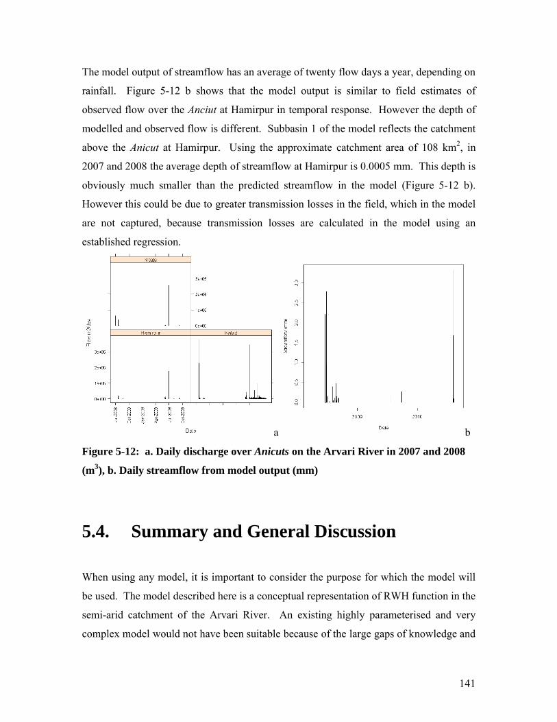
141
The model output of streamflow has an average of twenty flow days a year, depending on
rainfall. Figure 5-12 b shows that the model output is similar to field estimates of
observed flow over the Anciut at Hamirpur in temporal response. However the depth of
modelled and observed flow is different. Subbasin 1 of the model reflects the catchment
above the Anicut at Hamirpur. Using the approximate catchment area of 108 km2, in
2007 and 2008 the average depth of streamflow at Hamirpur is 0.0005 mm. This depth is
obviously much smaller than the predicted streamflow in the model (Figure 5-12 b).
However this could be due to greater transmission losses in the field, which in the model
are not captured, because transmission losses are calculated in the model using an
established regression.
a b
Figure 5-12: a. Daily discharge over Anicuts on the Arvari River in 2007 and 2008
(m3), b. Daily streamflow from model output (mm)
5.4. Summary and General Discussion
When using any model, it is important to consider the purpose for which the model will
be used. The model described here is a conceptual representation of RWH function in the
semi-arid catchment of the Arvari River. An existing highly parameterised and very
complex model would not have been suitable because of the large gaps of knowledge and

142
data related to the Arvari River catchment. This includes incomplete knowledge of
aquifer properties, a lack of basic hydrological data, including long term weather
observations in the catchment, soil properties and a gauging station on the river. In
contrast, simpler existing models do not incorporate the hydrological processes related to
RWH. As a result, a conceptual water balance model was purpose built. The model
captures the relevant hydrological processes in the catchment that are influenced by
RWH, which have not been captured appropriately in other models. This includes
surface water – groundwater interactions and large recharge volumes from the specific
land use – RWH.
Despite the aim to keep the model simple, the field results (Chapter 4) indicated that
some complexity and variability was necessary to capture the processes effectively in the
model. As such, the model has 23 parameters (Table 5-10). Compared to a simple model
such as IHACRES (Evans and Jakeman 1998), with only six parameters, it is more
complex. However low parameter models do not include the processes that are related to
RWH. Simpler models, while effective for modelling streamflow output do not allow
investigation of catchment internal hydrological processes. Those models that do include
a reservoir model and surface water – groundwater interactions, such as SWAT (Arnold
and Fohrer 2005), are far to complex (over 41 parameters) and data intensive. However
the semi-distributed, deterministic model built here is similar in structure to models like
SWAT. A study by Ye et al (1997) compared three rainfall-runoff models including
GSFB (8 parameters), IHACRES (6 parameters), and a complex conceptual model,
LASCAM (22 parameters). They found that while the simple conceptual model is
adequate for monthly time periods, on a daily time step a slightly more complex model is
better for prediction of streamflow in an ephemeral catchment. As the model built here
was on a daily time step, in order to capture the recharge process from RWH, it is
comparable to LASCAM in complexity.

143
Table 5-10: Model Parameters and values
Model
ComponentParameter Name Value
Groundwater Percolation Coefficient 0.001 – 0.002
Initial Value 100 mm
Maximum Value 200 mm
Parameter to describe flow
unit2/day/distance ()Eq 5-3
Elevation of Subbasin 1 (E1)
D2 Groundwater level in subbasin 2
D1 Groundwater level in subbasin 1
Rainfall (P) Rainfall Depth Varies with each year
Rainfall Length 0.5 in monsoon, 0.06 in dry months
Evapotranspiration
(ET)
Critical available water AWcr 0.7 FC Agric, 0.78 FC for Commons
Wilting point (WP) 0.454 FC Agric, 0.54 FC Commons
Leaf area index (LAI) Table 5-2
Light use efficiency (-c_T) 0.4
Soil moisture stress function ( ) (Eq 5-5)
Root fraction (fr) 1
RWH HRU Hydraulic conductivity Ksat 1534.28 mm/day
Depth to groundwater table (L) 18000 mm Johads, 4000 mm Bandhs
Maximum storage depth 1000 mm Johads, 2000 mm Bandhs
Threshold for recharge non-linearity 100
a (shape parameter) 0.3
HRUs (Ag1, Ag2,
Ag3, Commons)
Curve Number (CN) Table 5-6
Field capacity (FC) Agric 261 mm, Commons 100 mm,
Irrigation Trigger (Ag2, Ag3) When soil profile is AWcr
The model described in this Chapter is similar to many other conceptual models purpose
built to address a specific hydrological issue (Table 5-11). For example a similar semi-

144
distributed, semi-conceptual model, using linear reservoirs and with surface water –
groundwater interactions, was built to examine flooding in the Okavango Delta,
Botswana, though on a monthly time step (Wolski, Savenije et al. 2006). Another study
uses a conceptual model due to a data poor environment in Ghana, to estimate runoff in
small reservoirs, using the Thornthwaite-Mather procedure, which represents the runoff
process occurring in this area. This model was calibrated by using remotely sensed
reservoir storage changes, a method which could also be applied in the future to the
model developed here (Liebe, van de Giesen et al. 2009). The TEDI model (Lowe,
Nathan et al. 2005) and the HYLUC-Cascade model (Bishop, Calder et al. 2009)
represent similar hydrological processes to estimate the impact of farm dams on
catchment flows, but do not incorporate any surface water – groundwater interactions.
Table 5-11: Comparison of the model described in Chapter 5 with well established models
Model NameNumber of
ParametersLimitations
Chapter 5
Model23 Not calibrated or validated to field measurements
IHACRES 6 Limited surface water – groundwater interaction
SWAT 41 Highly complex, requires large data inputs
TEDI 5 No surface water – groundwater interactions
Admittedly the model in this study is only a conceptual representation of the actual
environment of the case study. As a result, there is uncertainty in the representation of
the landscape described in this chapter and the model output could not be applied to the
field. This includes uncertainty in operations (data missing, human error), input
(estimates) and hydrologic uncertainty (model and calibration). However, because the
model focuses on conceptual relationships and there is limited data, uncertainty
estimation is not possible. Future work would be to compare the output from this model,
with other more established models and greater data input to calibrate and validate, and
also whether those models are equifinal.

145
The sensitivity analysis identified the key data input that would have to be collected to
apply this model to a real catchment. To calibrate and validate the model output data
needed would be detailed streamflow data, and groundwater levels. Input data required
would be long-term series of spatial rainfall and runoff measurements to calculate
appropriate curve numbers. Key information for modelling of the internal processes
would be: land use patterns and ET distributions, soil properties and aquifer
characteristics. A longer time series of recharge estimates from RWH and natural
recharge estimates would also be valuable.
R, an open source statistics and mathematics program, was useful to develop the
conceptual model presented above, with a run time of 6 minutes if run for 10 years on a
daily time step through the whole catchment (1.7 GHz Pentium IV machine with 1 GB
RAM). While the model will produce results that are based on physical processes, they
are not an exact representation of reality, but give a general indication of trends of
changing land use and watershed development. The next step is to apply this model to
different scenarios to examine the impacts of RWH at the catchment-scale.

146
6. MODELLING RWH IMPACTS IN A
CATCHMENT – SIMULATION
ANALYSIS
6.1. Introduction
Sustainable water resource systems are those systems that are designed and managed to
contribute fully to the objectives of society, now and in the future, while maintaining
their ecological, environmental and hydrological integrity (Loucks and Gladwell 1999).
However trying to apply and quantify sustainability is difficult, because systems and the
‘needs’ are always changing (Sarang, Vahedi et al. 2008). Nevertheless a number of
studies have tried to quantify the sustainability of water resource systems by quantifying
measures of reliability, resilience and vulnerability. The indices are based on whether a
specified demand threshold is met by the water resource system (Hashimoto, Loucks et
al. 1982; Loucks 1997; Zongxue, Jinno et al. 1998; McMahon, Adeloye et al. 2006;

147
Ajami, Hornberger et al. 2008). These indices are used in conjunction with the
conceptual model discussed in Chapter 5 to examine the impacts of RWH in a catchment.
Two different aspects of the impact of RWH will be considered in this chapter. The first
examines the impact of RWH on irrigated agriculture using the sustainability indices. In
India irrigated agriculture is largely dependent on groundwater use. The impacts of
RWH on groundwater supply and thus irrigated agriculture are therefore an important
consideration. The amount of water needed to meet crop water requirements, which
includes water from groundwater and rainfall, is defined as the calculation of the
sustainability indices. This approach is purely anthropocentric because the threshold
considers only crop water demand, and ignores environmental and ecological ‘demands’.
A larger analysis examining these factors could be part of future work. The second
analysis investigates the changes in the catchment hydrology through examination of
changes in streamflow for different land use scenarios.
6.2. Methods
6.2.1. Sustainability Indices
Hashimoto et al. (1982) describe three criteria for evaluating the performance of water
resource systems:
1. How likely the system is to fail or the frequency of failure (Reliability, RE).
2. How quickly it recovers from failure (Resilience, RS), and
3. How severe the consequences or extent of failure may be (Vulnerability, V).
These measures are related to Holling’s seminal paper (1973), who first described the
concept of resilience as the ability of an ecological system to persist with the same basic
structure when subjected to stress. In order to quantify these indices, the operational
status of the water resource system needs to be described as either satisfactory (S) or
unsatisfactory (F), using defined thresholds. Unsatisfactory status could be the result of

148
floods, droughts, or higher demands. As Loucks (1997) points out, these thresholds are
subjective judgments. However by using these indices, improvements or trends in
different management scenarios can be gauged in a water resource system. These indices
are also easy to use (Kay 2000). For this reason they are used in this analysis to examine
the impacts of RWH for different areas of irrigation and RWH using the conceptual
model developed in Chapter 5.
1. Reliability (RE)
Reliability is the frequency or probability that a system is in a satisfactory state
(Fowler, Kilsby et al. 2003):
[ ]tprob X S where1
T
ttZ
RET
Eq 6-1
Where Xt is the system’s output state or status at time t, Zt is a binary measure where Xt is
either an element of S values (output or performance of the water resource system is in a
satisfactory state) or F values (output or performance of the water resource system is in a
failure state). The RE index ranges from 0 to 1, where 1 reflects 100% reliability in
meeting demands.
2. Resiliency (RS)
Resiliency is the probability that when a system is in a failure state, the next time step
is a satisfactory state (Fowler, Kilsby et al. 2003; Ajami, Hornberger et al. 2008):
1{ | }t tprob X S X F where
1
1
T
tt
T
t
WRS
T Zt
Eq 6-2
W = 1 if Xt is element of F and then Xt+1 is an element of S otherwise W = 0. The
resilience index ranges from 0 to 1, where 1 is a system with 100% resilience.

149
3. Vulnerability (V)
Vulnerability is the maximum of the sum of the difference between the threshold
(criteria – C) and the actual level (Xt) for any failure periods (Ji) (Fowler, Kilsby et al.
2003; Ajami, Hornberger et al. 2008).
max , 1,...,i
tt J
V C X i N
Eq 6-3
It thus reflects the severity of the failure. The vulnerability index can have a wide range
depending on the difference between Xt and C, but higher values indicate higher
vulnerability, lower values represent a less vulnerable system.
Many studies have used these three indices to evaluate the sustainability of water
resource systems. Fowler et al. (2003) modelled the impacts of climate change on the
resilience of the Yorkshire water resource system. Kay (2000) applied the performance
indices to the crop production index of Israel to examine Israel’s water resource system
from 1949-1997. Jain and Bhunya (2008) used the indices with Monte Carlo simulations
to test the performance of a reservoir in India. Peters et al. (2005) investigated how
droughts are changed by groundwater systems and analysed the performance of
groundwater during drought. And finally Ajami et al. (2008) used the indices to examine
how hydrological uncertainties impact the management system.
6.2.2. Defining thresholds
From the literature there is sufficient evidence to show that there is a direct link between
irrigation and poverty alleviation. Agricultural growth leads to overall economic growth,
and irrigation is a prime catalyst for agricultural growth. Groundwater development
increases irrigation area (Mukherji and Shah 2005) and is seen as a more effective way to
target poverty than surface irrigation, due to its reliability and spatial availability
(Wegerich 2006). There is also literature to support that where RWH is introduced,
irrigated agriculture increases. In Orissa, India, a study by Srivastava et al. (2008)

150
confirmed that farmers increased Rabi and Zaid crops in the 2nd and 3rd year after RWH
was established. The study found that a rain-fed farmer will shift to irrigated agriculture
once the reliability of the groundwater system is established. Therefore the thresholds for
the calculation of the sustainability indices in this study relate to water demand for
irrigated agriculture.
In the Arvari River catchment, irrigation is supplied mainly through groundwater.
However the water requirement for the first crop season (Kharif) is primarily met by
rainfall. If rainfall requirements are not sufficient, then they are supplemented with
groundwater where possible. The winter crop season (Rabi) is completely reliant on
groundwater for irrigation. The summer season (Zaid) is generally 10% or less of the
irrigated agriculture area and is also completely reliant on groundwater for irrigation.
Because of the small area of Zaid, the thresholds are only defined for water required to
irrigate the Kharif and Rabi crops.
In the study area the main crop grown during Kharif is maize. For maximum production
a medium maturity grain crop requires between 500 to 800 mm of water depending on
the climate. The water required to irrigate maize using the FAO crop factors, is
511.8 mm for 125 growing days (Allen, Pereira et al. 1998). The main Rabi crop is
wheat. For high yields, water requirements are 450 to 650 mm depending on the climate
and length of the growing period. For the model a threshold of 470.5 mm of water for
120 growing days of wheat was used (Allen, Pereira et al. 1998).
To meet crop water demands, the farmers rely on a combination of groundwater and
rainfall in Kharif and groundwater in Rabi. The water resource system in this study was
therefore based on the availability of water in the sowing months of the Kharif (July) and
Rabi (November) crops. The available water in the system is defined daily as the
groundwater storage combined with any rainfall in the months of July (Kharif) or
November (Rabi). More months were not considered, because the initial water available
at the start of each season strongly determines water availability for the rest of the season
and the amount of irrigated area planted as observed in the field (Chapter 4), so any

151
impact of RWH would best be seen in these months. The water available in these months
was then compared with the defined threshold to calculate daily values of the
sustainability indices.
6.2.3. Simulations
Due to the stochastic generation of rainfall in the model, 30 realisations of the rainfall
were applied to each land use scenario for the whole catchment (Figure 6-1). The model
was run on a daily step for 12 years. The first two years of the model were discarded
before the analysis as a ‘warm-up period’. A number of different land use scenarios were
considered based on the area of irrigation, the area of RWH and whether irrigation or
RWH is present. The percentage area of RWH land use varied at 0.5%, 1%, 1.5% and
3% and the irrigated land use percentage area was varied at 5%, 10%, 15% and 20%.
Scenarios were run with and without irrigation and RWH. Results are presented as
box-plots, which present the distribution across the rainfall realisations, with medians,
and averaged across the subbasins.
Figure 6-1: Histogram of annual rainfall distribution (mm) for 30 realisations of 12
year model simulations in Subbasin 2

152
6.2.4. Droughts
In the Arvari River catchment, groundwater supply is not only affected by the irrigation
demand, (represented as the area under irrigation) and recharge from RWH, but also by
the amount of rainfall. While irrigation area and RWH area are determined by societal
management actions, rainfall in the area is an exogenous variable. Drought is a
temporary, recurring meteorological event, which begins because of a lack of
precipitation and results in a lack of water availability for natural resources and human
activities, particularly agriculture (Smakhtin and Schipper 2008).
Drought affects each component of the water balance differently, but the analysis here
considers the impact of drought on the modelled groundwater output to meet irrigation
demand. To understand the influence of annual rainfall and drought conditions on
irrigated agriculture and RWH, simulations of drought were run, where a drought year
was defined as below average annual rainfall. The model was run incorporating different
lengths of years of below average rainfall. The indices were compared between each of
the drought scenarios. For example the model was run for 12 years; 3 yrs of above
average rainfall, then a below average rainfall period, which ranged from 2 to 6 years,
then another 3 yrs of above average rainfall and so on until the end of the 12 year time
period was reached. The first two years of the model were again discarded for the
analysis.
6.2.5. Streamflow changes
With increasing RWH land use in a catchment, flow downstream may change as more
runoff is stored in RWH structures. This will be examined in the model by examining
differences in streamflow between different scenarios of RWH and irrigation area. In
particular differences in the rainfall-runoff relationship will be analysed, including any
reduction in streamflow depth and amount.
153
6.3. Results
6.3.1. The System without RWH
Figure 6-2 shows the results of the sustainability indices for scenarios without RWH,
with 4 different irrigation areas. All indices show that as the area of irrigation increases,
sustainability decreases in the system. A greater area of irrigation represents a greater
crop water demand and therefore more groundwater extraction would occur, so that the
threshold is not met as frequently as at a smaller irrigation area.
Reliability clearly shows the impact of the increase in irrigation area, which drops from a
reliability of 0.8 at 5% irrigation, to half that at 10% irrigated area (Figure 6-2 a). This
difference is not as large from the 15% to 20% irrigated area, because the reliability is
already very low at 15%. Resilience again is highest for the smallest irrigated area, but as
irrigation area increases, the decrease in the RS index increases is not as much as the RE
index, because RS is already low at a small area of irrigation (Figure 6-2 b). This
indicates that the overall capacity of the system to withstand shocks is minimal.
Vulnerability increases with increasing irrigation, and is highest at 20% irrigation,
reconfirming what the other indices show (Figure 6-2 c).
The Rabi season has higher reliability, resilience, and lower vulnerability than the Kharif
season, which is a reflection of the threshold defined for each season, which is higher for
Kharif than Rabi (Section 6.2.2).

154
a. b
c
Figure 6-2: Distribution of the sustainability indices, with median, for different
areas of irrigation without RWH for Kharif and Rabi a. Reliability Index,
b. Resilience Index, c. Vulnerability Index
6.3.2. The System with RWH
When RWH is introduced in the model the indices indicate a more viable water resource
system for irrigated agriculture, compared to the previous analysis without RWH. This is
indicated by overall higher reliability and resilience, and lower vulnerability.

155
There is not much difference in reliability as irrigation increases in the Kharif and Rabi
seasons (Figure 6-3). In both crop seasons, at 5% and 10% irrigation, the impact of
RWH means that these scenarios are almost completely reliable. Even though reliability
decreases at 15% and 20%, it is still greater than scenarios without RWH (Figure 6-2).
As RWH area increases (x-axis in Figure 6-3), reliability increases, but at 15% and 20%
irrigation area, as RWH increases from 1.5% to 3%, reliability does not increase further
and slightly decreases, particularly at the 20% irrigation area in the Rabi season (Figure
6-3).
Figure 6-3: Distribution of the reliability index with median for different areas of
irrigation and RWH for Kharif and Rabi season
The 5% irrigation scenario does not have a calculated resilience index, because there
were no failure states from which to return to a satisfactory state (Figure 6-4). 15% and
20% irrigation areas have low resilience values (Figure 6-4). However these values are

156
higher than in the scenarios without RWH, so a system with RWH is more resilient than
without RWH.
At 10% irrigation, in both crop seasons, the resilience index behaves quite differently to
the other scenarios (Figure 6-4). This is the result of the irrigation area function in the
model that mimics farmer behaviour in the field, which relates the fraction of irrigated
land to the groundwater level. If water is plentiful (defined in the model as the shallow
aquifer level higher than 125 mm) then the defined fractional area of irrigated agriculture
increases 1.2 times. This function is thus a distinct ‘step’ function, which creates an
abrupt change in the irrigation area. A smooth function would be more suitable, but due
to lack of information on the exact shape of such a function, this was not attempted. In
the 5% irrigation area scenario the groundwater level is always above 125 mm, and in the
15% and 20% irrigation area scenarios, the groundwater level is always below 125 mm.
However at the 10% irrigation area scenario, the function impacts the resilience index.
At 10% irrigation, in the Rabi season, at 0.5% RWH area, the groundwater levels are
greater than 125 mm, so the fraction of irrigation area does not increase and resilience is
high. However as RWH area increases, the groundwater levels increase due to increased
recharge, and the irrigation area function begins to operate, increasing the irrigation area,
which in turn decreases groundwater levels and thus the resilience index. At 3% RWH
the irrigation area function can only increase the irrigation area to a maximum 1.2 times
or 12%, so extraction can not increase further, and because of additional RWH the
resilience increases. This is similarly reflected in the Kharif season at 10% irrigation
area, except that the function is also operating at 0.5% RWH because of the rainfall input
in this crop season, which increases storage into RWH and thus recharge.

157
Figure 6-4: Distribution of the resilience index with median for different areas of
irrigation and RWH for Kharif and Rabi season
Vulnerability, or the extent of failure, is predictably highest when irrigation area is largest
(20%). A larger area of irrigation means a larger volume of water is pumped from the
groundwater. Therefore the difference between the demand required and the available
water is greater, giving a higher vulnerability. At low irrigation area (5%), vulnerability
is negligible, but increases with each increasing step of irrigation area. At 20% irrigation,
as RWH area increases, the vulnerability distribution is similar for all RWH values.
However at 15% irrigation, in both crop seasons, as RWH increases from 0.5% RWH to
1% area, vulnerability increases. And from 1.5% to 3% RWH area, the vulnerability
does not improve much (Figure 6-5). This is also seen at 10% irrigation in the Kharif
season, which shows a similar response for the same area for the Rabi season in the
reliability analysis that is the result of the irrigation area function operating.

158
Figure 6-5: Distribution of the vulnerability index with median for different areas of
irrigation and RWH for Kharif and Rabi season
Compared to the first analysis with irrigation and no RWH (Figure 6-2), the addition of
RWH in the system increases reliability, resilience and decreases the vulnerability of the
water resource system for irrigated agriculture. Within an individual irrigation scenario,
as RWH area increases from 1.5% to 3%, the benefit to the system is not large and in
some cases the sustainability indices actually decrease. This suggests that there is a
limiting point in the area of RWH that gives a maximum benefit for recharge, beyond
which the benefit is marginal. In addition the fact that farmers respond to water levels
and increase their irrigation area means that some levels of RWH area have less
sustainability.
159
6.3.3. The Influence of Rainfall
To understand the influence of variations in annual rainfall on irrigated agriculture and
RWH, the indices were compared between below average and above average annual
rainfall years. The long-term average from the Thanagazi station data of 705.8 mm was
taken as the average for this analysis. The analysis shown here is for the Rabi season
only, as the Kharif season displays a similar response. Also the Rabi season has less
daily rainfall, so the impact of recharge from RWH would be the primary influence on
whether the threshold demand is met or not.
In all indices, the above average rainfall years show higher sustainability than below
average rainfall years. Systems with and without RWH have higher reliability with
above average rainfall (Figure 6-6). However when rainfall is below average, the
reliability of the system with RWH performs better than a system without RWH. This is
seen most clearly at 5% and 10% irrigation scenarios; in this case, despite below average
rainfall, the system has almost 100% reliability. The reliability of a system without RWH
has median reliability of 80% for 5% irrigation area and 20% for 10% irrigation area
(Figure 6-6 a and b). When rainfall is above average, RWH in a system gives 100%
reliability up to the 15% irrigation scenario (Figure 6-6 b). In the below average rainfall
scenarios when RWH is present the change from 1.5% RWH to 3% RWH sees a slight
decrease in reliability (Figure 6-6 b).

160
a b
Figure 6-6: Reliability in Rabi with below average rainfall and above average
rainfall a. without RWH at various levels of irrigation, b. with various scenarios of
RWH and irrigated agriculture
Resilience is also better with above average rainfall (Figure 6-7). Again a system with
RWH has better resilience than a system without RWH (Figure 6-7 b). With RWH in the
system and above average rainfall, resilience can not be measured for 5%, 10% irrigation
scenarios. As RWH increases from 1.5% to 3% no large improvements in the index
value is seen. At 10% irrigation in the below average rainfall with RWH (Figure 6-7 b)
the results are similar to Figure 6-4, which is the result of the irrigation area function
operating. Groundwater levels are low at 0.5% RWH so the irrigation area does not
increase, and resilience is high. From here, as RWH area increases, resilience decreases
because groundwater levels rise and the irrigation area function is operating. In Figure 6-
7 a, despite the absence of RWH, because of above average rainfall, groundwater levels
increase, so that at 10% and 15% irrigation, the irrigation area function works, while at
20% groundwater levels are not high enough to trigger the irrigation area function, and so
resilience is higher.

161
a b
Figure 6-7: Resilience in Rabi with below average rainfall and above average
rainfall a. without RWH at various levels of irrigation, b. with various scenarios of
RWH and irrigated agriculture
In Figure 6-8 the vulnerability index shows that a system with RWH is better than a
system without RWH in above and below average rainfall years. In Figure 6-8 b as
RWH increases, vulnerability is similar for all levels of RWH.
In this analysis when rainfall is below average, the sustainability indices are not as
positive as when rainfall is above average, due to lower recharge from RWH. However
in below average rainfall, the indices are greater with RWH in the system than without
RWH. This means RWH alleviates some of the deficit in below average rainfall years
because it supplies some groundwater, though it would be less than in an above average
rainfall year. This was observed in Chapter 4 in the difference in potential recharge
volume between the two different rainfall years.

162
a b
Figure 6-8: Vulnerability in Rabi with below average rainfall and above average
rainfall a. without RWH at various levels of irrigation, b. with various scenarios of
RWH and irrigated agriculture
6.3.4. Drought Conditions and RWH Impact
RWH provides within season buffering, but may not provide longer term supply if
drought occurs, because the pumping for irrigation reduces the buffer between seasons
and recharge from RWH would decrease.
The overall sustainability indices for 10 year time period, with increasing series of
concurrent below average rainfall years, does not show strong differences as the drought
period increases. This suggests that RWH is able to provide some buffer in low rainfall
periods (Figure 6-10). Overall the resilience index is low, but it shows some change,
with decreasing resilience as the drought period increases, and also the reliability
decreases as drought period increases, but these changes are not as large as when RWH is
not present in the system in the analysis in section 6.3.1.

163
a b
c
Figure 6-9: Sustainability indices in simulations with a. 2 year drought period, b. 4
year drought period, c. 6 year drought period
6.3.5. Streamflow Impacts of RWH
Figure 6-10 displays plots of annual streamflow as a percentage of rainfall against annual
rainfall for different areas of RWH and irrigation. When irrigation is introduced, the
gradient of the rainfall – streamflow relationship decreases, but streamflow still occurs at
low annual rainfall. As irrigation area increases, the large streamflow events decrease.
This is because the model converts the Commons HRU, with a higher CN, to irrigated

164
HRUs, which has lower runoff. Therefore more water is ‘captured’ through irrigated
land use, and ‘blue’ water is converted into ‘green’ water.
When RWH is introduced the gradient increases, but streamflow does not start until an
annual rainfall of about 500 mm, compared with Figure 6-10 a and b, when streamflow
starts around an annual rainfall of 400 mm. In the model, RWH captures runoff that
would otherwise reach the stream and so the amount and frequency of water entering the
stream decreases. Smaller rainfall events are captured, but larger events overflow from
the RWH structures and move into the river. If the RWH area is increased (Fig 6-10 d),
the percentage amount of streamflow events decrease further, but the greatest change in
streamflow occurs from 0% RWH area to 0.5% RWH area (Table 6-1).
Table 6-1 also shows the large impact RWH has on streamflow, by decreasing the mean
and maximum, and increasing the intercept. The mean runoff coefficient, defined as the
% rainfall converted to streamflow, decreases dramatically when a small level of RWH is
developed in the system.
Table 6-1 Analysis of streamflow with different scenarios of RWH and irrigation
Scenario Linear Model Streamflow as % Rainfall
RWH %
Area
Irrigation
% AreaSlope
x axis
interceptMean
Standard
DeviationMaximum
0 0 0.017 194 7.0 2.7 19.6
0 15 0.011 118 5.4 1.7 16.5
0.5 15 0.021 486 2.9 2.8 18.3
1 15 0.021 524 2.0 2.7 17.0
1.5 15 0.021 524 1.6 2.7 16.3
3 5 0.024 422 4.4 3.1 17.4
3 10 0.023 513 2.2 2.9 16.1
3 15 0.019 526 1.2 2.4 14.9

165
a b
c d
e f
Figure 6-10: Annual streamflow as % of annual rainfall (mm) a. No RWH or irrigated
agriculture, b. 15% Irrigated Agriculture, No RWH, c. 15% Irrigation, 0.5% RWH,
d. 15% Irrigation, 3% RWH, e. 5% Irrigation, 3% RWH, f. 10% Irrigation, 3% RWH

166
6.4. Discussion
At present irrigated agriculture in India is far more reliant on groundwater than the earlier
rain-fed systems. As a result of this dependence the groundwater resource has become
overexploited in some areas, so that the groundwater buffer, which provides resilience
against shocks such as drought, no longer exists (Moench 2007). Agricultural drought
occurs widely in India, with about 68% of net sown area highly vulnerable. Most of this
area is located in arid and semi-arid areas, where frequent and prolonged drought results
in lowered groundwater levels (Mudrakartha 2007). This chapter indicates that increased
recharge through RWH is an important element for providing some resilience against
shocks such as drought in a groundwater irrigated agriculture system.
Under RWH scenarios irrigated agriculture is more viable than in a system without
RWH. However the analysis also showed that continuously increasing RWH area does
not bring additional benefits that may be expected. Instead as RWH area increases, the
system reaches a limiting point, from where the benefit from RWH does not increase the
sustainability indices, and in some cases decreases. This is because runoff from a
catchment area is finite and more RWH means that water is just spread across more
storage area. As a result, the resulting depths in the RWH structures are smaller and the
recharge per structure decreases. Recharge can not increase beyond a certain limit for
each structure storage area and can not be greater than Ksat. Additionally the aquifer
storage capacity is limited. This relationship was seen for an individual structure by
Sharda et al. (2006) and in this study (Section 4.2.2.2). It is very interesting to note that
this same limiting capacity is also seen when RWH is examined at the catchment-scale.
Additionally if the area of irrigation is large (in this analysis up to 20% of the catchment
area), RWH many not be able to reduce the stress on the water resource system, because
demand is too large.
The result from this analysis that increasing RWH beyond a certain point, does not
increase the benefit to irrigation, could have serious impacts for NGOs, other agencies

167
and communities that invest in RWH, because the benefit to agriculture may not be worth
the cost of additional RWH works at high levels of RWH development in a catchment. A
greater understanding of this limiting capacity could aid in RWH development programs.
This reinforces theoretical speculations about catchment-scale impacts of RWH by
Kumar et al. (2006), which considered a higher degree of RWH development to reduce
marginal benefits, while increasing marginal costs. That paper understood that reduction
in benefit to be because of low aquifer storage capacity, lower chances of getting
appropriate sites for RWH development, and the environmental costs of RWH. The
model used in this study has a small aquifer storage capacity, but has also found that the
nature of runoff and storage in RWH structures is an important consideration in the
reduction in benefits of recharge from RWH. The model is conceptual, so before further
recommendations, these results must be compared with other models that have been
calibrated and validated to a specific catchment, which would require additional data.
The analysis from the model in this chapter confirms that RWH increases the viability of
groundwater irrigated agriculture if short-term mild drought conditions occur. However
from this analysis, longer term drought does not seem to strongly decrease the function of
RWH. Kumar et al. (2006) say that RWH has extremely limited potential to provide
reliable water supply, because of high rainfall variability and high PotET but the analysis
from this chapter shows that while the sustainability indices decrease when drought
occurs, the system is functioning better than without RWH.
Another important aspect of RWH impacts is the hydrological changes in a catchment,
which were examined by comparing streamflow changes under different scenarios. The
model clearly shows that when RWH is introduced, streamflow strongly decreases.
Capturing local runoff upstream in RWH storages addresses problems of frequent
drought and widespread poverty in upper catchments. However the ‘blue’ water
investments, like irrigation canals, are generally located downstream (for example
Sainthal Sagar Dam in the Arvari River catchment) and depend on large volumes of
runoff (Sakthivadivel 2008). As RWH leads to an increase in water used for irrigated
agriculture upstream, this will affect water availability for other downstream users,

168
including not only irrigators but also ecosystems, because flows, which are already highly
variable in a semi-arid region, decrease. However RWH could also have positive
environmental impacts as result of reduced land degradation, for example in the Arvari
River catchment, more area has been re-forested since RWH development as the
community recognises the importance of erosion control. There could also be
improvements in water quality as runoff is slowed through the catchment, so larger
sediments would filter out and the erosive power of the flows is reduced. This would
require further field analysis to investigate.
The scenarios of irrigation area and RWH area highlight the link and strong feedbacks
between irrigation area and RWH. The model does not capture fully the changing
dynamics area of irrigation. Realistically, if groundwater levels were low, farmers might
also reduce the area of irrigation, alleviating further pressure on the groundwater
resource. While the model results show that RWH has a positive impact for the
sustainability of irrigated agriculture, if the supply of groundwater increases due to RWH,
then local demands may also increase unsustainably. This depends on how groundwater
is managed, which is considered in Chapter 7.

169
7. MANAGEMENT OF
GROUNDWATER DEMAND IN THE
ARVARI RIVER CATCHMENT
7.1. Introduction
The introduction of RWH clearly has an impact on local groundwater tables (Chapter 4),
and is therefore an important tool to increase local groundwater supply. However
groundwater institutions, which regulate and monitor the use of groundwater, also are an
important influence on the dynamics that govern the sustainability of this resource. In
India, the institutional arrangements related to groundwater do not prevent unrestricted
use, which is partly due to the nature of the resource itself. Aquifers are often large and
invisible, which means it is difficult to exclude other users. Despite the large size, the
supply is limited; consumption by one user reduces its availability to others (Ostrom,
Gardner et al. 1994). These management difficulties are exacerbated by the millions of

170
wells that exist in India and the structure of groundwater property rights. In India
groundwater property rights are attached to land, allowing land owners to extract
groundwater as economically possible (Saleth 2005).
Groundwater use has exponentially increased in the last 50 years in India, but well-
constructed institutions to manage this resource have not yet been developed (Kemper
2007) and the current top-down approach to manage groundwater has not been
successful, with water levels declining in many states (Rodell, Velicogna et al. 2009).
Giving resource property rights to communities, so that it is managed as a commonly-
owned or common property resource (CPR), has been encouraged as an alternative to
effectively manage resources like groundwater, particularly in developing countries
(Berkes 1989; Bromley 1992; Ostrom, Walker et al. 1992; Bruns 2007; Moench 2007).
But there are very few documented examples of successful commonly owned
groundwater institutions, and relatively little is known about those institutions that do
exist and how they govern groundwater use (Mukherji and Shah 2005). This chapter
therefore examines one such CPR institution in the Arvari River catchment, the Arvari
River Parliament (ARP), initiated in 1998 with the help of Tarun Bharat Sangh (TBS),
the local NGO (Non-Government Organisation).
Secondary sources and a small number of structured interviews will be used to examine
the ARP. The researcher interviewed a number of farmers within the Arvari River
catchment during the data collection period. Inclusion criteria were based on whether
they were actively participating in the ARP, via their respective Gram Sabha (village
councils), whether they are living in the catchment and use groundwater. Participants
were approached directly and asked if they would like to participate. Six interviews were
held with members of the ARP and their respective Gram Sabhas and five interviews
with groundwater users who are not members of the ARP, but owned wells that were
close to RWH structures. Ethics approval was obtained for these interviews.

171
7.2. Inception and Rules of the Arvari River
Parliament (ARP)
Since 1987, TBS has been building RWH structures with the local community. TBS
works in villages after being approached by a village community for support. For each
structure that is built, the village community covers a proportion of the construction
costs; either monetarily or through voluntary labour. Where structures are built, TBS
encourages the formation of a Gram Sabha (village council), to discuss where the
structures ought to be built and how the structures would be maintained. The general
results of RWH for communities in this area have been very positive. Moench, Dixit et al
(2003) found that 85% of RWH structures have benefited small and marginal farmers by
increasing groundwater supplies. This has allowed farmers to increase the area under
irrigation and decrease their dependency on the rain-fed Kharif crops. Until 1996 there
were no catchment-scale management plans in place.
In 1996, a conflict between State Government officials from the State Fisheries
Department and the village of Hamirpur led to the formation of the Arvari River
Parliament. In 1995, a large Anicut was built on the river reach at Hamirpur, which held
a substantial amount of water. In November 1996 the State Fisheries Department gave
licenses to fish in the Anicut to a Jaipur contractor. The village people opposed the
contractor. The community felt that because they had built the RWH structure that held
the water, the government did not have the authority to decide how that water could be
used.
“When there was no water, where was the government? We requested and
appealed many times to the government. But they did not listen to us; they did not do
anything to provide us with water. Now, we have water because of the efforts of TBS and
ourselves. All of us worked hard without any government support. Our efforts were not
supported by the government even though it was the responsibility of the government.
Therefore the government has no right to give fishing-contracts for our water”
(from interview with Gram Sabha member, 2008).

172
With the support of TBS, the villagers held a Satyagraha (non-violent protest) against the
State Fisheries Department for two months. The result was that the fishing contracts
were cancelled in March 1997.
Due to this incident the community and TBS realised that others outside the community
could use the water provided through RWH, which were considered the common
property of each village. Consequently in December 1998, TBS called representatives of
all Gram Sabhas of the Arvari River catchment to a meeting, where the ARP was
initiated. On January 26 1999 the ARP was officially affirmed. The ARP has 110
representatives from the 72 villages of the Arvari River catchment (Kumar and Kandpal
2003).
The rules of the ARP were first set up in 1998, and focus mainly on water conservation
and utilisation and forest conservation. All members agree to enforce the following
informal rules:
Water intensive crops like sugarcane, rice and cotton are not to be planted
No one shall draw water from the river or RWH structures. But those people who
gave their land for RWH structures or whose land is under water because of
RWH, can take water from RWH structures and the river
No commercial fishing is allowed in water stored in RWH structures
Tube wells, which tap deeper aquifer, are not allowed
Construction and maintenance of RWH is encouraged
Land is not to be sold for mining/quarrying or any other industrial activity
Protection and planting of forests in encouraged
These informal rules are discussed at each biannual meeting to highlight practical
problems in their implementation and suggest new guidelines if needed (Moench, Dixit et
al. 2003). Suggestions, if any, are debated and discussed. Members also seek guidance
for resolving conflicts, if any, and report any violations of the rules listed above (Singh
2005). The informal rules are then conveyed downwards to individual villages through
the elected Gram Sabha representatives. These are then discussed and implemented at

173
the village level either through social or moral pressure, depending on the activeness of
each village Gram Sabha.
7.3. Review of the ARP
Despite the presence of the informal rules of the ARP, unrestricted use of groundwater
still occurs within the Arvari River catchment. This is due to a number of factors
including information problems about the resource size and capacity. Monitoring use of
a resource that is easily accessed, yet invisible, also has high transaction costs because it
would be difficult to monitor without understanding the capacity of the resource and the
number of users. As highlighted earlier in Chapter 3, scientific information about
hydrogeological properties or boundaries in this area is not readily available. Depending
on the size of the aquifer, farmers using groundwater may not have any appropriation or
provision problems until irrigation is fully established, and only then may they be
motivated to work together (Schlager 2007). While all interviewees considered the
amount of groundwater available a problem, they all considered that to be dependent on
the amount of rainfall, rather than the area of irrigation or amount of groundwater
extraction. Those interviewees who were members of the ARP believed more RWH
structures ought to be built to alleviate any groundwater shortage. Decreasing or limiting
groundwater extraction was not considered by anyone interviewed. The solution to limit
extraction of groundwater could be to limit well building, which for people in this
catchment, who are dependent on groundwater for their livelihood, might not be an
attractive solution. Annual fluctuations are very strong (as seen in Chapter 4) due to the
shallow aquifer system that most farmers in this area access. This reflects the amount of
rainfall, so the aquifer may self-limit extraction.
The only groundwater demand rules in the ARP apply to crop choice. Crops are visible,
and so it is easy to see whether other users are abiding by the informal rule to not plant
certain crops. However, the interviews and other literature suggest that most people in

174
the Arvari River catchment are not aware of the ARP or its rules (Kumar and Kandpal
2003). From the interviews, the five farmers who were not members of the ARP and
owned wells near RWH structures had not heard of the ARP. And of those, four were
unaware of a Gram Sabha in their village. While the rules suggest no new tube wells to
be built, there are no direct restrictions on dug well drilling or pumping. And in 2007
new tube wells seen while monitoring, and in one village three new tube wells had been
installed in the last three years. There is nothing to stop well owners from deepening
existing wells, digging new wells, or increasing pump capacity. The researcher also saw
pumping occurring directly from the river and from the storage of the Anicut at Kaled in
2008, despite the ARP informal rule that pumping should not take place in the river or
from RWH storage (with exceptions).
Enforcement and monitoring of the rules depends on the strength of the moral sanctions
within the community. This depends on the activity and strength of the Gram Sabha to
convey the ARP informal rules to the village community. A recent evaluation of TBS’s
work found that most Gram Sabhas remained dormant after TBS had withdrawn from the
village after construction of RWH. However in some villages, the Gram Sabha had taken
up further activities (Kumar and Kandpal 2003). Where the Gram Sabha is most active,
there has been significant impact on the management of common resources, such as
forests, grazing lands and RWH construction and maintenance (Moench, Dixit et al.
2003). The most active Gram Sabhas were found in villages at the upper end of the
catchment. The percentage of land under RWH in these areas is higher than other areas
on lower elevations. These landscape positions also mean that RWH has had the largest
impact on groundwater tables, for example in Bhaonta village, and so the community is
more likely to work collectively because of the individual benefit from working together.
The ARP is evaluated against Ostrom’s factors that favour collective action (Table 7-1)
(Ostrom 1990; Ostrom 1992; Ostrom 2000). These factors have been used to evaluate
water institutions in a number of studies including Lopez-Gunn and Cortina (2006) and
Lopez-Gunn (2003), which evaluated groundwater user associations in Spain. But the
use of these factors prescriptively or interpreting them too simplistically has been debated

175
(Cleaver and Franks 2005; Bruns 2007; Moench 2007). Cleaver and Franks (2005)
consider these factors too limited with simplistic assumptions about the users, between
the rules and the decision making structures. Nevertheless the design principles do
outline key challenges facing the users for collective action, but are insufficient by
themselves to suggest solutions. In the context of the ARP, the design factors are used to
provide a framework for analysing and highlighting the challenges facing the Arvari
River catchment community to manage groundwater.
As can be seen from Table 7-1, the ARP does not have many of the factors that Ostrom
considers to favour collective action. While each user is heavily dependent on the
resource, the boundaries are not clear. New users can only be excluded if they do not
own land, as groundwater rights legally lie with the land. There is no structured
monitoring of the resource or operational rules regarding the amount of groundwater
extraction, so ‘free riding’ still occurs, which could further discourage collective action
(Schlager 2007). When asked about the impacts of pumping, all interviewees described
water levels going down locally as water is pumped, but larger or longer-term aquifer
impacts were not mentioned.

176
Table 7-1 Analysis of ARP and the factors that favour collective action (Ostrom
1990; Ostrom 1992)
Attributes Characteristics of the Arvari River Parliament
Clearly defined
boundaries
The ARP is defined based on surface water boundaries of the Arvari
River, not groundwater boundaries. Aquifer boundaries are not clearly
defined.
Salience High dependency of the groundwater resource by users for their
livelihood.
Participation of
most users
Participation is dependent on the activity of Gram Sabhas, which are
more active in the upper catchment. Most people in the catchment are
unaware of the ARP, but there is no restriction to membership. All
members are small holder farmers who use groundwater. The average
age is in the mid forties, and there are very few female representatives.
Users bound by
mutual
obligation
There is no obligation between users to restrict the use of groundwater.
Any restriction depends on the activeness of the Gram Sabha and moral
sanctions within the village community.
Common
understanding of
the resource
The general perception of groundwater from the interviews was that
pumping effects local supply, but depends on the internal routes of
groundwater. Shortage of groundwater is felt to be related to rainfall.
Impacts of individual use are not well understood on long term and
larger scale aquifer capacity.
Graduated
sanctions
There are no graduated sanctions. Enforcement and monitoring at
village level through moral sanctions and pressure, which depends on the
Gram Sabha activity.
Leadership Strong local charismatic leader since inception.

177
Attributes Characteristics of the Arvari River Parliament
Prior
organisational
experience
None, but TBS volunteers, who have some experience, participate in the
ARP.
Technical
Capacity
No specific scientific information on aquifer characteristics available,
and what information is available is held with higher agencies. Users
have long term experience of groundwater behaviour in their wells.
There is no information on the number of wells in the catchment, their
locations, or extraction.
Financial
Capacity
None, because there are no overheads. There is no membership fee.
TBS provides lunch at the biannual meetings.
Autonomy The ARP has no de jure rights. The external authorities are not aware or
do not acknowledge the ARP.
Currently the Arvari River catchment is not facing serious supply issues in groundwater.
This is because the farming practices are such that the level of irrigation does not have
large or strong negative impacts on other users in the catchment. Also the resource itself
encourages self-limiting behaviour in pumping. Most farmers access the shallow aquifer
through dug wells, which varies significantly within a year. Consequently irrigation area
fluctuates depending on the level of water at the end of each monsoon. As population
grows and more area is developed for irrigation, perhaps longer term water table decline
patterns could appear. However this would require reliable information, and due to the
lack of monitoring in the catchment this may be difficult to determine. Nevertheless the
ARP could provide a forum through which members can discuss such issues if they
occur. More importantly the institution could act as a lobby and empower users to
exclude other larger users of groundwater from entering the catchment, for example
industrial units. Greater understanding of the resource capacity and user pumping

178
impacts at the catchment community level would greatly improve the ability of the
community and an institution like the ARP to encourage monitoring of groundwater.
The ARP encourages the implementation of RWH across the catchment. All
interviewees, when asked about the downstream impacts of RWH, said that any impact
would be positive, because groundwater would move towards them in the aquifer. Strong
lateral flow was also suggested in the field analysis in Chapter 4, with almost 30% of
potential recharge from RWH structures moving away laterally in the unsaturated zone of
the shallow aquifer. So while RWH works are carried out at the village scale, the water
stock that the village would hope to access from the construction of RWH, may not be
exclusive to the group of users who initiated RWH. Instead that water may move away
or could even be pumped away from the control of that group, if there is no physical
boundary. By encouraging RWH across the catchment, any movement of groundwater
away from some users could be balanced by more RWH construction upstream. From
Chapter 4 in this area the effects of RWH are largely local, and in the upper rockier areas
of the catchment, wells almost 6 km away are influenced by recharge from RWH.
However, the model simulations suggest that RWH impacts reach a maximum level of
efficiency beyond which the benefit decreases, i.e. the cost-benefit ratio increases to a
point beyond which the benefits do not warrant the cost (Chapter 6). This consequence
means that demand-side management of groundwater would be better targeted to manage
groundwater supply.
7.4. Conclusion
As highlighted in the example of the Arvari River Parliament, a community-based
approach to manage groundwater in India faces serious challenges and constraints,
largely because of the lack of information for resource users about the resource. Despite
this, knowledge and impact of institutions at the operational level are important,
particularly in India, where millions of wells exist. As Shah (2007b) points out, for

179
community-based institutions to work, it must serve a private purpose important to the
users, otherwise they may not all participate or may even try to work against it. Currently
in the Arvari River catchment that private purpose is not present, because dug well tap
the shallow aquifer, which fluctuates annually and is largely dependent on rainfall and
recharge from RWH (Chapter 4). But if irrigation area and population pressure increases,
and more tube wells are sunk, then perhaps the need for collective action will arise, and
an institution like the ARP will have more relevance. At this time the need for reliable
information about aquifer characteristics and user behaviour will be important for the
ARP to function effectively. If groundwater shortage does becomes a serious problem in
the future, then change in livelihood patterns from the current heavy dependence on
irrigated agriculture would ultimately be necessary to alleviate further extraction of
groundwater.

180
8. KEY FINDINGS, IMPLICATIONS
AND DISCUSSION
The purpose of this thesis was to investigate the impacts of RWH, specifically designed
to increase groundwater recharge, as this is important for effective implementation of
watershed development programs in India. In this chapter, the key research findings of
the thesis are summarised, implications for watershed development are explored, and the
limitations of the study are presented. As this thesis is a step towards greater
understanding of RWH, it also suggests the way forward for future research in this topic.
The major contribution from this study is a methodology to systematically examine the
impact of RWH development in a catchment.

181
8.1. General Overview and Key Findings
The thesis presented here examines the main question:
What are the impacts of rainwater harvesting (RWH) at the local and catchment
scales?
The key components of this work are:
1. As a case study, local-scale impacts of RWH were examined in the Arvari River
catchment in 2007 and 2008. Rainfall and water levels in RWH structures and
dug wells were measured as part of an extensive monitoring approach.
2. A conceptual model was developed to specifically investigate RWH impacts at
the larger catchment-scale. This model incorporates the main hydrological
processes influenced by RWH, inferred from the local-scale impact study.
3. Different RWH and irrigated land use scenarios were simulated in the conceptual
model to examine catchment-scale impacts of RWH on irrigated agriculture and
streamflow.
4. The ability of the community-based institution, the Arvari River Parliament, to
manage groundwater demand was analysed.
The case study confirmed the strong local-scale impacts of RWH on groundwater levels
that has been referred to in a number of studies (Gore, Pendke et al. 1998; Sharda,
Kurothe et al. 2006). The measured catchment rainfall displayed large variability, which
locally influenced the storage of RWH and thus potential recharge volume from an
individual RWH structure. This was particularly noticeable between rainfall years, where
2008 was a comparatively wetter year and had higher potential recharge volumes than
2007. Depending on structure size and landscape position RWH potential recharge
varied. Potential recharge from RWH was highest from Anicuts on the river, and the
Bandhs had a higher volume of potential recharge than Johads. In total RWH
contributed about 7% of rainfall to potential recharge in the catchment, which was similar
in both rainfall years, despite the difference in rainfall between years. This is due to

182
RWH structure shape and size, landscape position and underlying stratigraphy, which are
the main factors that influence RWH performance. However this level of potential
recharge did not translate into the actual recharge from the analysis of the groundwater
levels in the dug wells. This is likely due to a number of elements including; local
mounding of the water table beneath RWH structures, storage in the soil profile, and high
lateral flow in the aquifer. This resulted in much lower actual groundwater recharge
levels. There are strong annual variations in the water levels in all the dug wells,
including those not close to RWH structures, particularly between the pre- and post-
monsoon season levels. While this study has not quantified the impact of an individual
RWH structure on groundwater levels, because of the number of structures and the few
observation wells in the field study, judging by the strong local influence of recharge near
RWH structures, and the small natural recharge estimates from literature, the results
suggest that RWH most likely influences groundwater levels across the shallow aquifer.
The results from the field study add to the knowledge base of local-scale RWH impacts
in India, which are limited in the literature. The results also compare well with the few
previous local scale studies of RWH such as Sharda et al. (2006). Overall the story from
the field data is one of high spatial and temporal variability. However the results also
clearly confirm the effectiveness of RWH performance to produce groundwater recharge.
Catchment-scale impacts of RWH are an area of research that has been little investigated.
This study examines this research question through the use of a water balance model.
However an analysis of existing water balance models showed that most had high
complexity and large data requirements. Given the lack of information and lack of long
term data series in the Arvari River catchment, a conceptual model was developed. The
model incorporates the main hydrological processes relevant to RWH and those that
influence catchment hydrology. This was inferred from the case study field data and
local observations. The main purpose of the model was to improve the understanding of
the feedbacks in the water balance related to RWH, and to explore the data inputs that
would be required to apply such a model to a specific catchment. The model uses
hydrological response units (HRUs) based on land uses of RWH, agriculture (including
irrigated area) and Commons land use. Agricultural and Commons HRUs have a specific

183
soil layer, curve number for runoff and leaf area index for the plant species. Recharge for
RWH is not based on the water balance method, as it is for the other HRUs, but uses
Darcy’s Law. Rainfall was applied stochastically in the model. The model was
calibrated qualitatively based on the local-scale field data in the Arvari River catchment.
The main difficulties in simulating the hydrological processes from the field in the model
were capturing the non-linearity of RWH recharge, and simulating the management
practices where irrigation area is a function of groundwater levels.
The literature review and observations from the case study catchment describe a strong
link between RWH area and the opportunity for increasing irrigated land use. Often
RWH is implemented to augment groundwater supply, which is then extracted for
irrigation. The model simulations showed that as the RWH area increases, groundwater
supply increases, and thus the potential for larger areas of agriculture to be irrigated.
This link was analysed using sustainability indices developed by Hashimoto et al. (1982)
for different land use scenarios. The results show that irrigated agriculture is more viable
with RWH than without as indicated. However as the area of RWH increases, there is a
maximum limit to the benefit from RWH, as at greater RWH areas, the captured runoff is
divided over a greater RWH storage area. In this study the maximum benefit limit is
somewhere between 1% and 3% RWH area. This limit was also displayed in the field
study for an individual structure, where for each structure a maximum recharge limit was
reached. The results of the resilience index at 10% irrigation highlight the impact of
increasing irrigation area when there is sufficient groundwater. Such management
practices may increase crop yields, but the viability of the water resource system
decreases at the optimal level of RWH found in the model. The presence of RWH
decreases the impacts of short-term mild drought situations. Finally, at the
catchment-scale, the model showed that as RWH increases, downstream flow decreases,
and the runoff coefficient decreases strongly when a small area of RWH is introduced in
the model. These conclusions have important management implications.
Implementation of RWH addresses supply-side issues of groundwater, while demand
management of groundwater is reliant on the human institutions that develop rules to

184
manage groundwater extraction. The Arvari River Parliament was examined to see if this
institution could regulate and monitor groundwater demand, but despite its efforts,
unrestricted groundwater use occurs. The major limitation for this group is primarily the
private purpose for the users to work collectively and secondly the lack of scientific
information about the aquifer properties, including size and capacity. Any groundwater
shortage issues are considered to be related to rainfall, mainly because groundwater users
tap the shallow aquifer, which has strong local annual variability. As a consequence
RWH is seen as a solution to groundwater shortages, rather than restricting groundwater
extraction, which for most users in the catchment is their main livelihood. Nevertheless
operational-level management of groundwater is an option that ought to be explored
further due to the difficulties of managing this resource at larger administrative scales.
8.2. Implications
In India groundwater irrigation has helped to alleviate poverty and increase rural growth,
but groundwater is being consumed unsustainably (Rodell, Velicogna et al. 2009).
Groundwater decline is a serious concern, particularly for small-holder farmers which are
disproportionately dependent on the resource (Gale, Neumann et al. 2002). Consequently
RWH has been implemented as part of larger watershed development programs and has
been initiated by communities, NGOs and government agencies across the country to
augment groundwater supply. While RWH development has visible impacts on
groundwater levels, very few studies have examined in detail the local-scale impacts of
RWH and the hydrological processes associated with RWH. Instead RWH seems to have
been implemented in a rather rapid, unplanned, and unregulated manner. For example
RWH in the Arvari River catchment was driven by local demand at the village level,
rather than planned at an aquifer or river catchment level. However the success of RWH
work in this area is because of focus at the village-scale. In addition the ARP was set-up
once the community saw the need for an integrated approach to watershed development.

185
Catchment-scale impacts of RWH are even less investigated and understood locally, but a
growing body of scientific literature is beginning to highlight the need for such research.
The thesis presented here has further highlighted these issues and increased the body of
knowledge about RWH. The study gives estimates of potential recharge from different
types of RWH in a semi-arid catchment in Rajasthan, and the translation of these
potential values into actual groundwater rise. Communication of these outcomes to the
local community is one of the follow-up priorities.
Each RWH structure has a limiting capacity to induce maximum recharge, which
depends on structure size and shape, the rainfall – runoff characteristics of the catchment
and hydrogeological properties of the area. In the case of the Arvari River catchment,
RWH structures in the higher elevations and on the river have a larger potential recharge
impact than smaller structures on lower elevations. Therefore the positioning of
structures in a landscape is important when investing in RWH. In the Arvari River
catchment, these components were addressed in RWH construction by villagers, whose
local experience of landscape conditions guided the choice of suitable sites and structure
types appropriate for their needs. However at the catchment-scale, the modelling results
describe a similar limiting capacity of RWH to induce recharge beyond a certain
maximum. When the area of RWH was doubled in the modelled conceptual catchment,
the benefit to irrigated agriculture, using the sustainability indices, was not substantial,
but the decrease in streamflow was stronger. This has important implications for NGOs,
communities and government agencies who build RWH structures, because the cost of
investing in RWH may not equal the benefit gained from this investment, and the
downstream streamflow impacts would be more widely felt. These results deserve more
consideration by applying the model to a specific catchment, and particularly examining
the aquifer properties, because the case study results suggest that despite surface flows
decreasing downstream when RWH is implemented, downstream users could possibly
benefit from lateral flow of groundwater.

186
8.3. Limitations and further research
Semi-arid rural areas are generally data sparse environments and the Arvari River
catchment is no exception. As a result, the field data collection was limited in scope due
to the conditions and infrastructure in the catchment area and the size of the project
resources. Nevertheless the results are comparable to the smaller scale and more data
intensive study of Sharda et al. (2006). Consequently the thesis shows that basic field
information is equally capable to provide estimates of RWH characteristics. A more
detailed future field study could try to identify the minimum dataset needed to
characterise local and catchment-scale impacts of RWH. It could also examine a larger
area of the specific catchment, which in this study was focussed in the middle and upper
reaches of the catchment. This would account for more variability in the catchment. A
climate station, a river gauging station and a longer time series of data would be very
valuable, as well as greater knowledge of aquifer properties and characteristics.
Installation of piezometers across the catchment would alleviate some of the pumping
issues associated with the dug wells in this study. Additionally soil water characteristics
could be measured in RWH storage areas to better estimate soil water storage. These
measurements could then possibly be used in a 2D soil-water model to calculate recharge.
Rainwater harvesting may also act as erosion control by reducing runoff velocities, soil
erosion, and sediment loads. This could have further ecological benefits for the
catchment ecosystem as more water would be available for a longer time. Therefore
runoff could be gauged by using RWH structures storage for events of rainfall, which in
this study was taken on a daily time step. Also future work could examine sediment
loads received in RWH structures, and the necessary maintenance times for de-silting
structures could be calculated.
The model used in this thesis is conceptual so the next step would be to apply the model
to a specific catchment, which has a sufficiently long data time series, including rainfall,
groundwater levels, and river discharge, to allow effective calibration and validation.
The results of the simulation study could then be compared to the situation in a ‘real’

187
catchment. Additionally the output of the model could be compared with more complex
existing models if the data requirements are met. The complexity of the developed model
could also be increased to address the cost-benefit questions related to RWH and
irrigation development. This would mean including a crop growth model to simulate
crop yields. From modelled crop yields, income generation for the community could be
estimated. If such components are added, then rather than using sustainability indices,
the resilience of the socio-ecological system with RWH could be analysed. A socio-
ecological system would incorporate not only irrigated agriculture and the resultant
income from crop yields, but also the environment including riverine ecology and
environmental flows in the river. This could also possibly address issues related to
sediment loads and water quality. The socio-ecological system and the feedbacks
between RWH, irrigated agriculture and groundwater extraction could then be analysed.
The use of remote sensing including Landsat imagery could also be used and would help
in delineating land uses and could also be used to identify the number of RWH structures
and storage area surface areas in different years (Liebe, van de Giesen et al. 2009). GIS
would be a useful tool in developing spatial layers of such data. Terrain attributes and
DEM information could also help with empirical modelling of the groundwater table.
8.4. Concluding comments
As pumping technology has changed, groundwater use has increased the accessibility of a
reliable source of irrigation water for small-holder farmers across India, alleviating
poverty in many rural areas. Yet the presence of millions of wells has meant that
groundwater is over extracted and water levels are declining. As a result RWH has been
widely implemented to raise deepening groundwater levels, but with no scientific or
hydrological studies to confirm or aid in implementation.
This study has therefore examined RWH in the semi-arid rural Arvari River catchment,
and then up-scaled the field results to the catchment-scale using a conceptual water

188
balance model developed in R to examine any hydrological impacts. This study has
shown that RWH has a positive impact on groundwater recharge, but decreases
streamflow downstream. Future work is needed to examine the conclusion drawn from
the simulation study, that increasing RWH ad infinitum does not increase benefit for
irrigation. Rainwater harvesting also changes blue water into green water as the
irrigation area increases as RWH is implemented.
Regardless of whether or what area of RWH is implemented, the institutions that manage
groundwater need to be established for sustainable use of the resource. These institutions
have particular relevance because increased recharge from RWH is strongly linked with
increased irrigation area, and the impact of such management practices can decrease the
resilience of the system.
The heavy reliance of groundwater in many parts of India means that the examination of
RWH impacts must be examined further for effective catchment development programs
in India, and the results should be conveyed to the groundwater users themselves.

189
APPENDIX 1 – PHOTOS AND MAPS OF
MONITORED RWH STRUCTURES
Photos of RWH structures monitored, local elevation ASL and distance of wells from
structures. Letters with the maps and photos relate to Table 4-1.
a b
c

190
d e
f g
h i

191
j k
l m

192
APPENDIX 2 – R CODE OF MODEL
SUBBASIN 1
# -----------------------------------## Subbasin 1 Variables# -----------------------------------#
#Landuse Area functionsag2 <- function(i) ifelse(year[i]>=Irrstart & (GWstore>125) & (Ag3.Irr(i)==TRUE),ag2.init*1.2,ag2.init)Luse.fr.BND <- (Luse.fr.JHD/0.4)*0.6Luse.fr1.Ag2 <- function(i) ifelse(year[i]<Irrstart,0,ag2(i))Luse.fr1.Ag3 <- function(i) ifelse(year[i]<Irrstart,0,(ag2(i)/0.9*0.1))Luse.fr1.Ag1 <- 0.35Luse.fr1.Com <- function(i) ifelse(year[i]<Irrstart && year[i]<RWH.start,0.65,ifelse(year[i]<Irrstart, 0.65-(Luse.fr.JHD+Luse.fr.BND),0.65-(Luse.fr.JHD+Luse.fr.BND+ag2(i)+(ag2(i)/0.9*0.1))))
# Groundwater size and initial for the UPPER AQUIFER GW.max <- 200GW.init <- 100
#Irrigation ParametersIrrstop <- 2050Irrmax<- 150Irrmin<- 100Ag1.Irr <- FALSEAg2.Irr <- function(i) {ifelse (month[i]==7 || month[i]==8 || month[i]==9 || month[i]==11 || month[i]==12 || month[i]==1, TRUE, FALSE)}Ag3.Irr <- function(i) {ifelse (month[i]==7 || month[i]==8 || month[i]==9 || month[i]==11 || month[i]==12 || month[i]==1 || month[i]==3 || month[i]==4 || month[i]==5, TRUE, FALSE)}Com.Irr <- FALSE

193
# RWH size and initial water and yr startedRWH.start <- 2000RWH.stop<- 2050JHDmax <- 1000JHD.init <- 0BNDmax<-2000BND.init<- 0
# RWH recharge parametersbnd.gw <- 4000jhd.gw <- 18000bnd.Ks <- 1534.28 #van genuchten mm/day (~4cm/hr)jhd.Ks <- 1534.28 #70# (40%s, 35%c) 1534.28threshold <- 100a <- 0.3
# Agriculture and Commons soil layer PAWC.ag <- 261.2PAWC.com <- 100AWinit.ag<- 130AWinit.com<- 50
# Curve NumberCN.Ag1 <- function (i) ifelse(LAI.Ag1(i)<=0.1, 72, 77)CN.Ag2 <- function (i) ifelse(LAI.Ag2(i)<=0.1, 72, 77)CN.Ag3 <- function (i) ifelse(LAI.Ag3(i)<=0.1, 72, 77)CN.Com <- 79Ia <- 0.05 #EvapotranspirationLAI.Ag1 <- function(i) {ifelse (month[i]==7 || month[i]==8 || month[i]==9, 4, 0.1)}LAI.Ag2 <- function(i) {ifelse (month[i]==7 || month[i]==8 || month[i]==9 || month[i]==11, 4, ifelse(month[i]==10 || month[i]==12 || month[i]==1 || month[i]==2,5, 0.1))}LAI.Ag3 <- function(i) {ifelse (month[i]==7 || month[i]==8 || month[i]==9 || month[i]==11 || month[i]==3|| month[i]==4 || month[i]==5|| month[i]==6, 4, ifelse(month[i]==10 || month[i]==12 || month[i]==1 || month[i]==2,5, 0.1))}LAI.Com <- function(i) {ifelse (month[i]==7 || month[i]==8 || month[i]==9 || month[i]==10 || month[i]==11 || month[i]==12|| month[i]==1, 4,0.5)}fr <- 1 c_T <- 0.45 s_w.ag <- 0.454*PAWC.ag #loam s_w.com <- 0.541*PAWC.coms_star.ag <- 0.7*PAWC.ag #loam s_star.com <- 0.78*PAWC.com

194
#Lateral flow between Subbasins E1 <- 457000perc.coeff <- 0.0001soil.GW <- 3000
#Routingriver.length <- 5 #km excluding tributariesriver.area<-125000*10^6 #mm^2 5km * 25mk <- 5
# -----------------------------------## Water Balance Functions# -----------------------------------#
#Routing FunctionStream.Routing <-function(It,It1,Qt,k) { f <- function(Vup) (1.983*Vup^0.73) Vup <- rep(0,river.length) Tloss <- rep(0,river.length) for (i in 1:river.length) { Vup[i] <- ifelse(i==1,It1,Vup[i-1])-f(ifelse(i==1,It1,Vup[i-1])) Tloss[i] <- f(ifelse(i==1,It1,Vup[i-1])) } Q <-((It + It1-2*sum(Tloss,na.rm=TRUE)+ Qt*(2*k-1))/(2*k+1)) Q1 <- Q/river.area Q <- ifelse(Q1<0,0,Q1) Tl <- sum(Tloss, na.rm=TRUE)/river.area Tloss <- ifelse(Tl<0,0,Tl) Out<- c(Q,Tloss) return(Out) }
#RUNOFF CN.fun <- function(P,CN,Ia){ S <- 25400/CN-254 Roff <- ifelse(P<Ia*S,0,((P-Ia*S)^2)/(P+(1-Ia)*S)) return(Roff)}
# Actual EVAPORATRANSPIRATIONE_Teuling <- function(AW,s_w,s_star,pot_ET, LAI) { if(AW <= s_w) { beta_T <- 0 } else { if (AW <= s_star & AW > s_w) {

195
beta_T <- (AW-s_w)/(s_star-s_w) } else { beta_T <- 1 } } ET <- fr*beta_T*(1-exp(-c_T*LAI))*pot_ET return(ET)}
# Water Balance for HRUsWaterbalance <- function( P,ET,CN,Luse.fr,PAWC,AWinit,Irr=FALSE, LAI, s_w, s_star) { Roff <- sapply(P,CN.fun,CN=CN,Ia=Ia) if (Irr==TRUE) { if(AWinit<=s_star) #changed from 0.55 to s_star { Irra <- PAWC - AWinit Irrb <- ifelse(P < Irra,Irra-P,0) Irrc <- ifelse(Irrb*Luse.fr > GWstore,GWstore,Irrb) Irrav <- ifelse(Irrc >= Irrmax,Irrmax,Irrmin) } else { Irrav <- 0 } } else { Irrav <- 0 }
ETcalc <- do.call(E_Teuling,list(AW=AWinit,s_w=s_w,s_star=s_star,pot_ET=ET, LAI=LAI))AW <- ifelse(AWinit + P + Irrav - Roff - ETcalc >s_w, AWinit + P + Irrav - Roff - ETcalc ,s_w)
DD <- ifelse(AW>PAWC,AW-PAWC,0) AW <- AW-DD Roff <- Roff*Luse.fr DD <- DD*Luse.fr Irrav <- Irrav*Luse.fr Out <- c(Roff,DD,AW,ETcalc,Irrav) return(Out)}
# define a function for the RWHRWH.balance <- function(Ksat, RWHstore.init, rwh.GW,threshold, a, Input, ET, RWHmax) { Rep1 <- ifelse(((RWHstore.init+ rwh.GW)/(rwh.GW))< threshold, (Ksat*((RWHstore.init+ rwh.GW)/(rwh.GW))), ((threshold-(threshold^a))+(Ksat*((RWHstore.init+ rwh.GW)/(rwh.GW))^a))) Rep <- ifelse(Rep1 < RWHstore.init, Rep1, RWHstore.init) RWH <- ifelse(RWHstore.init + Input - ET - Rep > 0, RWHstore.init + Input - ET - Rep,0) overfl <- ifelse(RWH > RWHmax, RWH-RWHmax,0)

196
RWH <- RWH - overfl Out <- c(RWH,overfl,Rep,ET,Input) return(Out)}
# Groundwater balanceGW.balance <- function(GWstore,perc.coeff,Input,Irr, G.lat,GWmax) { D.GW.loss <- GWstore*perc.coeff GW <- ifelse(GWstore + Input - Irr - G.lat - D.GW.loss >0,GWstore + Input - Irr - G.lat -D.GW.loss,0) baseflow <- ifelse(GW > GWmax,GW-GWmax,0) # correct GW for baseflow GW.init <- GW - baseflow Out <- c(GW.init,baseflow, D.GW.loss) return(Out)}# calc flow btw upper aquifers# calc D1D1 <- function(soil.GW, GW, Input) { D1 <- soil.GW+(GW-Input) Out <- c(D1) return(Out)}#calc D2D2 <- function(soil.GW, GW, Input) { D2 <- soil.GW+(GW-Input) Out <- c(D2) return(Out)}#calc flow btw upper aquifersGW.flow <- function(p,E1,D2,D1) { flow <- p*(E1+D2-D1) Out <- c(flow) return(Out)}
# -----------------------------------## Rainfall Prediction Model# -----------------------------------#
#Rainfall FunctionPrecip <- function(time,alpha,lambda) { f_P<-round(rexp(time,lambda)) for (p in 1:length(f_P)) { if (p ==1) { if (f_P[p]>0) { R <- c(rep(0,f_P[p]),rexp(1,1/alpha)) } else {

197
R <- rexp(1,1/alpha) } } else { if (f_P[p]>0) { R <- c(R,c(rep(0,f_P[p]),rexp(1,1/alpha))) } else { R <- c(R,rexp(1,1/alpha)) } } }return(R[1:time])}
#Annual rainfall analysis from AlwarA.rain <- read.csv("alwar_yrly_P.csv")A.annual.m <- mean(log(A.rain[,2]))A.annual.sd <- sd(log(A.rain[,2]))year.R <- seq(1901,2002)N <- length(year.R)Rain_fun <- function(year,N) { cos1 <- cos(2*pi*year/N) sin1 <- sin(2*pi*year/N) cos2 <- cos(4*pi*year/N) sin2 <- sin(4*pi*year/N) cos3 <- cos(6*pi*year/N) sin3 <- sin(6*pi*year/N) out <- data.frame(cos1=cos1,sin1=sin1,cos2=cos2,sin2=sin2,cos3=cos3,sin3=sin3) return(out)}Rain_mat <- cbind(Rain_fun(year.R,N),Rain=A.rain[,2])lm3 <- lm(Rain ~ .,data=Rain_mat)
# Linear model btw annual rainfall and wet/dry season Thanagazirain <- as.data.frame(read.csv("thanagazi_P_stack_no1999.csv"))P <- rain$PMonth.T <- rain$monthMonth.T <- as.numeric(substr(as.Date(rain$date,"%d/%m/%Y"),6,7))rain$wetP<- replace(rain$P,(Month.T<6 | Month.T>9),NA)rain$dryP<- replace(rain$P,(Month.T>=6 & Month.T<=9),NA)annual <- aggregate(rain[,5:7],list(year=rain$year),sum,na.rm=TRUE)fit.w <- lm(annual[,3]~annual[,2])summary(fit.w)slope.w <- fit.w$coefficients[2]int.w <- fit.w$coefficients[1]
# Predict ANNUAL RAINFALL for MODELDate <- (seq(as.Date("2000/1/1"), as.Date("2012/1/1"), "days"))

198
year <- as.numeric(format(Date,"%Y"))days <- c(rep(c(366,rep(365,3)),3))N <- length(unique(year))Rain_mat <- cbind(Rain_fun(as.numeric(unique(year)),N),Rain=N)p.A.rain.dry <- exp(log(runif(8,300,500) + rnorm(8,0,A.annual.sd)))p.A.rain.dryp.A.rain.wet <- exp(log(runif(6,600,1000) + rnorm(6,0,A.annual.sd)))p.A.rain <- c(p.A.rain.wet[1:2],p.A.rain.dry[1:8],p.A.rain.wet[3:5])p.A.rain
# lambdalambda.w <- 0.5117967lambda.d <- 0.05969731lambda.d <- rep(lambda.d,N)lambda.w <- rep(lambda.w,N)
# alphaA <- as.data.frame(matrix(nrow=N, ncol=2))#A$alpha.w <- (int.w + slope.w*p.A.rain)/(122*lambda.w)A$alpha.w <- ifelse(((int.w + slope.w*p.A.rain)/(122*lambda.w))>11,(int.w + slope.w*p.A.rain)/(122*lambda.w),11) #rainy season has 122 daysA$alpha.d <- (p.A.rain-(int.w + slope.w*p.A.rain))/((365-122)*lambda.d)
#Predict daily RAINFALL for 3 subbasinsRain <- as.data.frame(matrix(nrow=length(Date),ncol=4))colnames(Rain)<- c("month","Zone1.P", "Zone2.P", "Zone3.P")Rain$month <- as.numeric(substr(as.Date(Date,"%d/%m/%Y"),6,7))model.w1 <- unlist(sapply(l,function(l) Precip(days[l], A$alpha.w[l], lambda.w[l])))model.d1 <- unlist(sapply(l,function(l) Precip(days[l], A$alpha.d[l], lambda.d[l])))wet1 <- replace(model.w1,(Rain$month<6 | Rain$month>9),0)dry1 <- replace(model.d1,(Rain$month>6 & Rain$month<9),0)Rain$Zone1.P <- wet1+dry1model.w2 <- unlist(sapply(l,function(l) Precip(days[l], A$alpha.w[l], lambda.w[l])))model.d2 <- unlist(sapply(l,function(l) Precip(days[l], A$alpha.d[l], lambda.d[l])))wet2 <- replace(model.w2,(Rain$month<6 | Rain$month>9),0)dry2 <- replace(model.d2,(Rain$month>6 & Rain$month<9),0)Rain$Zone2.P <- wet2+dry2
model.w3 <- unlist(sapply(l,function(l) Precip(days[l], A$alpha.w[l], lambda.w[l])))model.d3 <- unlist(sapply(l,function(l) Precip(days[l], A$alpha.d[l], lambda.d[l])))wet3 <- replace(model.w3,(Rain$month<6 | Rain$month>9),0)dry3 <- replace(model.d3,(Rain$month>6 & Rain$month<9),0)Rain$Zone3.P <- wet3+dry3
Rain1 <- data.frame(year=format(Date,"%Y"),date=Date, zone1=Rain$Zone1.P,zone2=Rain$Zone2.P,zone3=Rain$Zone3.P)Date1 <- as.Date(Rain1$date,"%d/%m/%Y")

199
plot(Date1, Rain1$zone1, typ="l")lines(Date1, Rain1$zone2, col="red")lines(Date1, Rain1$zone3, col="blue")rain <- Rain1
write.csv(rain,"zone_rain.csv",row.names=FALSE)
# -----------------------------------## Store Results of Model# -----------------------------------#
Zone1.Climate <- matrix(nrow=length(Date), ncol=3) colnames(Zone1.Climate) <- c("month","P", "pot_ET")Zone1.Out <- matrix(nrow=length(Date),ncol=20) colnames(Zone1.Out) <-c("Roff.Ag1","Re.Ag1","AW.Ag1","etag1","irrag1","Roff.Ag2","Re.Ag2","AW.Ag2","Et2","Irrav.Ag2","Roff.Ag3","Re.Ag3","AW.Ag3","et3","Irrav.Ag3","Roff.Com","Re.Com","AW.Com","ETcom","irrcom")Zone1.RWH.Out <- matrix(nrow=length(Date),ncol=10) colnames(Zone1.RWH.Out) <-c("JHD.depth","JHD.of","JHD.re","JHD.et","jhdinput","BND.depth","BND.of","BND.re","BND.et","bndinput")Zone1.GW.Out <- matrix(nrow=length(Date),ncol=5) colnames(Zone1.GW.Out) <- c("GW.init","basef","D.GW.loss","D1","GW")Zone1.Stream.Out<-matrix(nrow=length(Date),ncol=4) colnames(Zone1.Stream.Out) <- c("flow","volume.flow","routed","tloss")
# -----------------------------------## Define Date and Predict Potential Evaporation# -----------------------------------#
Date <- (seq(as.Date("2000/1/1"), as.Date("2012/1/1"), "days"))
#Predict Potential Evapotranspirationday <- c(rep(c(1:366,rep(1:365,3)),4),1:366,rep(1:365,2))cos1 <- cos(2*pi*day/365)sin1 <- sin(2*pi*day/365)cos2 <- cos(4*pi*day/365)sin2 <- sin(4*pi*day/365)cos3 <- cos(6*pi*day/365)sin3 <- sin(6*pi*day/365)lm3 <- lm(rain$pot_ET ~ cos1 + sin1 + cos2 + sin2 + cos3 + sin3)# Create newdata using the newdata functionyear <- as.numeric(format(Date,"%Y"))day2 <- vector()day2[1] <- 1for (i in 2:length(year)) { if (year[i] == year[i-1]) { day2[i] <- day2[i-1]+1 } else

200
day2[i] <- 1} # Predict pot_ET Zone1.Climate$pot_ET <- predict(lm3, newdata=ETfit(day2))pot_ET <- Zone1.Climate$pot_ETplot(pot_ET, type = "l")dm <- format(Date, "%d/%m")
# -----------------------------------## Call Rainfall # -----------------------------------#
prec <- as.data.frame(read.csv("zone_rain.csv"))Zone1.Climate$P <- prec$zone1#Zone1.P <- Zone1.Climate$P[-(1:731)]P <- Zone1.Climate$PZone1.Climate$month <- as.numeric(substr(as.Date(Date,"%d/%m/%Y"),6,7))month <- Zone1.Climate$month
# -----------------------------------## Run Model # -----------------------------------#
#Model Loopfor (i in 1:length(Zone1.Climate$pot_ET)) {# Groundwater GWstore <- ifelse(i==1,GW.init,Zone1.GW.Out[i-1,1])# Ag1 AWinit <- ifelse(i==1,AWinit.ag1,Zone1.Out[i-1,3]) Zone1.Out[i,1:5] <-Waterbalance(P[i],pot_ET[i],CN.Ag1(i),Luse.fr1.Ag1,PAWC.ag1,AWinit,Ag1.Irr, LAI=do.call(LAI.Ag1,list(i=i)), s_w=s_w.ag, s_star.ag)[1:5]# Ag2 if (year[i] < Irrstart) { Zone1.Out[i,6:10] <- rep(0,5) } else { AWinit <- ifelse(year[i]==Irrstart & day.E[i] == 1 ,AWinit.ag,Zone1.Out[i-1,8])Zone1.Out[i,6:10] <- Waterbalance(P[i],pot_ET[i],CN.Ag2(i),Luse.fr1.Ag2(i),PAWC.ag,
AWinit,Ag2.Irr(i), LAI.Ag2(i), s_w.ag, s_star.ag)[1:5] }# Ag3 if (year[i] <Irrstart) { Zone1.Out[i,11:15] <- rep(0,5) } else { AWinit <- ifelse(year[i]==Irrstart & day.E[i] == 1 ,AWinit.ag,Zone1.Out[i-1,13]) Zone1.Out[i,11:15] <- Waterbalance(P[i],pot_ET[i],CN.Ag3(i),Luse.fr1.Ag3(i),PAWC.ag,AWinit,Ag3.Irr(i), LAI.Ag3(i), s_w.ag, s_star.ag)[1:5] }# Commons AWinit <- ifelse(i==1,AWinit.com,Zone1.Out[i-1,18]) Zone1.Out[i,16:20] <- Waterbalance(P[i],pot_ET[i],CN.Com,Luse.fr1.Com(i),PAWC.com,AWinit,Com.Irr, LAI.Com(i), s_w.com, s_star.com)[1:5]

201
# JHD if (year[i] < RWH.start) { # no RWH built Zone1.RWH.Out[i,1:5] <- rep(0,5) # all values are 0 } else { # RWH have been builds JHDstore.init <- ifelse(year[i]==RWH.start & day.E[i] == 1,JHD.init,Zone1.RWH.Out[i-1,1]) JHDinput <- (Zone1.Out[i,1]*Rof.JHD.Ag1(i) + Zone1.Out[i,6]*Rof.JHD.Ag2(i) +Zone1.Out[i,11]*Rof.JHD.Ag3(i) +Zone1.Out[i,16]*Rof.JHD.Com(i))/Luse.fr.JHD Zone1.RWH.Out[i,1:5] <- RWH.balance(jhd.Ks, JHDstore.init, jhd.gw, thresholdj, a, JHDinput,pot_ET[i],JHDmax) }# BND if (year[i] < RWH.start) { # no RWH built Zone1.RWH.Out[i,6:10] <- rep(0,5) # all values are 0 } else { # RWH have been build BNDstore.init <- ifelse(year[i]==RWH.start & day.E[i] == 1,BND.init,Zone1.RWH.Out[i-1,5]) BNDinput <- (Zone1.Out[i,1]*Rof.BND.Ag1(i) + Zone1.Out[i,6]*Rof.BND.Ag2(i) +Zone1.Out[i,11]*Rof.BND.Ag3(i) +Zone1.Out[i,16]*Rof.BND.Com(i))/Luse.fr.BND Zone1.RWH.Out[i,6:10] <- RWH.balance(bnd.Ks, BNDstore.init, bnd.gw, thresholdb, a, BNDinput ,pot_ET[i],BNDmax) }# Groundwater GWinput <- ifelse(i==1, 0,Zone1.Out[i-1,2]+Zone1.Out[i-1,7]+Zone1.Out[i-1,12]+Zone1.Out[i-1,17]+ Zone1.RWH.Out[i,3]*Luse.fr.JHD + Zone1.RWH.Out[i,8]*Luse.fr.BND+ Zone1.Stream.Out[i-1,4]) if (i == 1) { Zone2.GW.Out[i,5] <- 0 G.lat <- 0 } else { G.lat <- Zone2.GW.Out[i-1,5] } Zone1.GW.Out[i,1:3] <- GW.balance(GWstore,perc.coeff,GWinput,sum(Zone1.Out[i,c(10,15)]), G.lat,GW.max) [1:3] Zone1.GW.Out[i,4] <- D1(soil.GW,GW.max,Zone1.GW.Out[i,1])# Stream Zone1.Stream.Out[i,1] <- ifelse(year[i]>=RWH.start, Zone1.RWH.Out[i,2]*Luse.fr.JHD + Zone1.RWH.Out[i,7]*Luse.fr.BND+ Zone1.Out[i,1]*(1-(Rof.JHD.Ag1(i)+Rof.BND.Ag1(i))) + Zone1.Out[i,6]*(1-(Rof.JHD.Ag2(i)+Rof.BND.Ag1(i)))+ Zone1.Out[i,11]*(1-(Rof.JHD.Ag3(i)+Rof.BND.Ag1(i)))+ Zone1.Out[i,16]*(1-(Rof.JHD.Com(i)+Rof.BND.Ag1(i)))+ Zone1.GW.Out[i,2], Zone1.Out[i,1]+Zone1.Out[i,6]+ Zone1.Out[i,11]+ Zone1.Out[i,16]+Zone1.GW.Out[i,2]) # Move routing within i loop Zone1.Stream.Out[i,2]<-Zone1.Stream.Out[i,1]*river.area #Routing for Zone 1 (volume) Qinit <- ifelse(i==1,1,Zone1.Stream.Out[i-1,3]) It1 <- ifelse(i==1,100,Zone1.Stream.Out[i-1,2]) Zone1.Stream.Out[i,3:4] <- Stream.Routing(Zone1.Stream.Out[i,2],It1,Qinit,k)[1:2]}

202
REFERENCES
Abbs, K. and M. Littleboy (1998). "Recharge estimation for the Liverpool Plains." Australian Journal of Soil Research 36: 335-57.
Adhikary, P. P., D. Chakraborty, et al. (2008). "Pedotransfer functions for predicting the hydraulic properties of Indian Soils." Australian Journal of Soil Research 46: 476-484.
Agarwal, A. and S. Narain, Eds. (1997). Dying Wisdom. Rise, fall and potential of India's traditional water harvesting systems. New Delhi, Centre for Science and Environment.
Agarwal, A. and S. Narain (1999). Making Water Management Everybody's Business: Water Harvesting and Rural Development in India. Gatekeeper Series. London, International Institute for Environment and Development.
Agrawal, A. and G. N. Yadama (1997). "How do local institutions mediate market and population pressures on resources? Forest panchayats in Kumaon, India." Development and Change 28(3): 435-465.
Agrawal, G. D. (1996). Evaluation of Water Conservation Efforts in 36 Villages of Alwar District. Alwar, Tarun Bharat Sangh: 21.
Ajami, N. K., G. M. Hornberger, et al. (2008). "Sustainable water resource management under hydrological uncertainty." Water Resources Research 44(W11406).
Alley, W., R. Healy, et al. (2002). "Flow and storage in Groundwater Systems." Science 296: 1985-1990.
Alley, W. and S. Leake (2004). "The Journey from Safe Yield to Sustainability." Ground Water42(1): 12-16.
Anbazhagan, S., S. M. Ramasamy, et al. (2005). "Remote sensing and GIS for artificial recharge study, runoff estimation and planning in Ayyar basin, Tamil Nadu, India." Environmental Geology 48(2): 158-170.
Anderies, J. M. (2005). "Minimal model and agroecological policy at the regional scale: An application to salinity problems in southeastern Australia." Regional Environmental Change 5(1): 1-17.

203
Anuraga, T. S., L. Ruiz, et al. (2006). "Estimating groundwater recharge using land use and soil data: A case study in South India." Agricultural Water Management 84(1-2): 65-76.
Arnold, J. G., P. M. Allen, et al. (1993). "A comprehensive surface-groundwater flow model." Journal of Hydrology 142: 47-69.
Arnold, J. G. and N. Fohrer (2005). "SWAT2000: current capabilities and research opportunities in applied watershed modelling." Hydrological processes 19: 563-572.
Badarayani, U., H. Kulkarni, et al. (2005). Groundwater recharge from a percolation tank to a Deccan basalt aquifer: a case study from western Maharashtra, India. International Symposium on Management of Aquifer Recharge ISMAR5. Berlin, Germany, UNESCO. Series on Groundwater No.13.
Badiger, S., R. Sakthivadivel, et al. (2002). Preliminary assessment of a traditional approach to Rainwater Harvesting and Artificial Recharging of Groundwater in Alwar District, Rajasthan. Annual Partners' Meet 2002, IWMI-TATA Water Policy Research Program: 1-18.
Barah, B. C. (1996). Traditional Water Harvesting Systems: An Ecological Economic Survey. New Delhi, New Age International Limited.
Bari, M. A., K. R. J. Smettem, et al. (2005). "Understanding changes in annual runoff following land use changes: a systematic data-based approach." Hydrological Processes 19: 2463-2479.
Batchelor, C., M. S. Rama Mohan Rao, et al. (2003). "Watershed development: A solution to water shortages in semi-arid India or part of the problem?" Land Use and Water Resources Research 3: 1-10.
Batchelor, C., A. Singh, et al. (2002). Mitigating the Potential Unintended Impacts of Water Harvesting. IWRA International Regional Symposium "Water For Human Survival". Hotel Taj Palace, New Delhi, India.
Beecher, H., I. Hume, et al. (2002). "Improved methods for assessing rice soil suitability to restrict recharge." Australian Journal of Experimental Agriculture 42: 297-307.
Beernaerts, I. (2006). An evaluation framework for groundwater recharge enhancement systems for improved irrigated agriculture Division of Information Technology, Engineering and the Environment Adelaide, University of South Australia. Master of Engineering (Hydrology andWater Resources): 86.
Bellot, J., A. Bonet, et al. (2001). "Likely effects of land use changes on the runoff and aquifer recharge in a semiard landscape using a hydrological model." Landscape and Urban Planning 55: 41-53.
Berkes, F., Ed. (1989). Common Property Resources. Ecology and Community-based Sustainable Development. London, Belhaven Press.
Beven, K. (2001). Rainfall-Runoff Modelling The Primer, Wiley: Chichester.

204
Bhuiyan, C., R. P. Singh, et al. (2006). "Monitoring drought dynamics in the Aravalli region (India) using different indices based on ground and remote sensing data." International Journal of Applied Earth Observation and Geoinformation 8(4): 289-302.
Bishop, E., I. Calder, et al. (2009). Development and application of the HYLUC-Cascade model for investigating the water resource impacts of rainwater harvesting structures in India. The Centre for Land Use and Water Resources Research. Newcastle, Newcastle University: 11.
Boers, T. M. and J. Benasher (1982). "A Review of Rainwater Harvesting." Agricultural Water Management 5(2): 145-158.
Bond, W. (1998). Soil physical methods for estimating recharge. Volume 3 Studies in Catchment Hydrology. THe basis of recharge and discharge. L. Zhang and G. Walker. Vicotria, CSIRO Publishing: 17.
Boudling, R. J. (1994). Description and Sampling of Contaminated Soils: a field guide, CRC Press.
Bouwer, H. (2002). "Artificial recharge of groundwater: hydrogeology and engineering." Hydrogeology Journal 10: 121-142.
Bredehoeft, J. D. (2006). "On Modeling Philosophies." Ground Water 44(4): 496-499.
Bromley, D. W. (1992). "The commons, common property, and environmental policy." Environmental and Resource Economics 2(1): 1-17.
Bromley, D. W. and D. Chapagain (1984). "The Village against the Centre: Resource depletion in South Asia." American Journal of Agricultural Economics 66: 868-873.
Brundtland, G. (1987). The World Comminssion on Environment and Development. Our Common Future. Oxford, Oxford University Press.
Bruns, B. (2007). Community Priorities for Water Rights: Some Conjectures on Assumptions, Principles and Programmes. Community-based Water Law and Water Resource Management Reform in Developing Countries. B. van Koppen, M. Giordano and J. Butterworth. Oxfordshire, CAB International
Calder, I., A. Gosain, et al. (2006). "Watershed development in India 2. New Approaches from managing externalities and meeting sustainability requirements." Environment, Development and Sustainability.
Chand, R., S. Chandra, et al. (2004). "Estimation of natural recharge and its dependency on sub-surface geoelectric parameters." Journal of Hydrology 299: 67-83.
Cleaver, F. and T. Franks (2005). How institutions elude design: river basin mangaement and sustainable livelihoods. Bradford, Bradford Centre for International Development: 21.
COMMAN (2005a). Community Management of Groundwater Resources in Rural India: Background papers on the causes, symptoms and mitigation of groundwater overdraft in India, British Geological Survey Commissioned Report CR/05/36N.

205
COMMAN (2005b). Managing Groundwater Resources in Rural India: the Community and Beyond, British Geological Survey Commissioned Report, CR/05/35N.
Costelloe, J. F., R. B. Grayson, et al. (2005). "Modelling stream flow for use in ecological studies in a large, arid zone river, central Australia." Hydrological Processes 19: 1165-1183.
Crosbie, R. S., P. Binning, et al. (2005). "A time series approach to inferring groundwater recharge using the water table fluctuation method." Water Resources Research 41.
Custodio, E. (2002). "Aquifer overexploitation: what does it mean?" Hydrogeology Journal 10: 254-277.
Datta, P. S. (2005). "Groundwater ethics for its sustainability." Current Science 89(5): 812-817.
de Vries, J. and I. Simmers (2002). "Groundwater recharge: an overview of processes and challenges." Hydrogeology Journal 10: 5-17.
Deb Roy, A. and T. Shah (2002). Socio Ecology of Groundwater Irrigation in India. Annual Partners' Meet 2002, IWMI-TATA Water Policy Research Program.
Dhawan, B. (1989). Studies in Irrigation and Water Management. New Delhi, Commonwealth Publishers.
Dhawan, B. (1995). Groundwater depletion, Land Degradation and Irrigated Agriculture in India. New Delhi, Commonwealth Publishers.
Dillon, P. (2005). "Future management of aquifer recharge." Hydrogeology Journal 13: 313-316.
Dunkerley, D. and K. Brown (1999). "Flow behaviour, suspended sediment transport and transmission losses in a small (sub-bank-full) flow event in an Australian desert stream." Hydrological Processes 13: 1577-1588.
Eggertsson, T. (1990). Economic behaviour and institutions, Cambridge University Press.
El-Hames, A. S. and K. S. Richards (1998). "An integrated, physically based model for arid region flash flood prediction capable of simulating dynamic transmission loss." Hydrological Processes 12: 1219-1232.
Evans, J. P. and A. J. Jakeman (1998). "Development of a Simple, Catchment-Scale, Rainfall-Evapotranspiration-Runoff Model." Environmental Modelling and Software 13: 385-393.
Falkenmark, M. (2003). "Freshwater as shared between society and ecosystems from divided approaches to integrated challenges." Philosophical transactions of the Royal Society of London B 358: 2037-2049.
Fernandez-Illescas, C. P. and I. Rodriguez-Iturbe (2004). "The impact of interannual rainfall variability on the spatial and temporal patterns of vegetation in a water-limited ecosystem." Advances in Water Resources 27: 83-95.
Finch, J. W. (1998). "Estimating direct groundwater recharge using a simple water balance model - sensitivity to land surface parameters." Journal of Hydrology 211: 112-125.

206
Fowler, H. J., C. G. Kilsby, et al. (2003). "Modeling the impacts of climatic change and variability on the reliability, resilience, and vulnerability of a water resource system." Water Resources Research 39(8): 1222-1233.
Gadjil, M. and P. Iyer (1989). On the Diversification of Common-Property Resource Use by Indian Society. Common Property Resources. F. Berkes. London, Belhaven Press: 240-272.
Gale, I. (2005). Strategies for Managed Aquifer Recharge (MAR) in semi-arid areas. IAH -MAR. Paris, France, UNESCO IHP.
Gale, I., I. Neumann, et al. (2002). The effectiveness of Artificial Recharge of groundwater: a review. Commissioned Report CR/02/108N. Nottingham, British Geological Survey: 1-50.
Gallant, J. C. and M. F. Hutchinson (2006). Producing digital elevation models with uncertainty estimates using a multi-scale Kalman filter. 7th International Symposium on Spatial Accuracy Assessment in Natural Resources and Environmental Sciences. M. Caetano and M. Painho. Lisbon, Portugal.
Gee, G. and D. Hillel (1988). "Groundwater recharge in arid regions: Review and critique of estimation methods." Hydrological Processes 2: 255-266.
Gee, G., Keller, J., Ward, A. 2005. "Measurement and predication of deep drainage from bore sediments at a semiarid site". Vadose Zone Journal. 4 (1). 32-40
Geological Survey of India (1999). District Resource Map, Alwar District, Rajasthan. A. K. Bhattacharya and S. S. Jain, Government of India.
Gheith, H. and M. Sultan (2002). "Construction of a hydrologic model for estimating Wadi runoff and groundwater recharge in the Eastern Desert, Egypt." Journal of Hydrology 263: 36-55.
Gontia, N. K. and R. S. Sikarwar (2005). "Rainwater harvesting and groundwater recharge in Saurashtra region of Gujarat - A success story." Indian Journal of Soil Conservation 33(3): 256-258.
Gopalakrishnana, C., C. Tortajada, et al., Eds. (2005). Water Insitutions: Policies, Performance and Prospects. Berlin, Springer.
Gore, K. P., M. S. Pendke, et al. (1998). "Groundwater modelling to quantify the effect of water harvesting structures in Wagarwadi watershed, Parbhani district, Maharashtra, India." Hydrological Processes 12(7): 1043-1052.
Gowing, J. W., H. Mahoo, et al. (1999). "Review of rainwater harvesting techniques and evidence for their use in semi-arid Tanzania." Tanzania Journal of Agricultural Science 2(2): 171-180.
Grafton, R. Q. (2000). "Governance of the commons: a role for the state?" Land Economics76(4): 504-517.
Grewal, S. S., S. P. Mittal, et al. (1989). "Rainwater Harvesting for the Management of Agricultural Droughts in the Foothills of Northern India." Agricultural Water Management 16(4): 309-322.
207
Grey, N. R. and O. P. Sharma (2005). Traditional rainwater harvesting technologies: key to drinking water security for desert communities in arid regions of India. International Symposium on Management of Aquifer Recharge ISMAR5. Berlin, Germany, UNESCO. Series on Groundwater No.13.
Grismer, M., S. Bachman, et al. (2000). "A comparison of groundwater recharge estimation methods in a semi-arid, coastal avocado and citrus orchard (Ventura County, California)." Hydrological Processes 14: 2527-2543.
Gronwall, J. (2006). Enforcement of groundwater rights in India: The Coca-Cola Case. Groundwater for Sustainable Development, New Delhi, India, Allied Publishers.
Ground Water Department Jodhpur (1999). Ground water resources Banganga River Basin. Jaipur, Government of Rajasthan.
Guntner, A., M. S. Karlo, et al. (2004). "Simple water balance modelling of surface reservior systems in a large data-scarce semiarid region." Hydrological Sciences Journal 49(5): 901-918.
Gupta, K. K., J. Deelstra, et al. (1997). Estimation of water harvesting potential for a semiarid area using GIS and remote sensing. Remote sensing and geographic information systems for design and operation of water resources systems. Proceedings of an International Symposium (5th Scientific Assembly of the IAHS), Rabat, Morocco, 23 April to 3 May 1997., IAHS Publ. 242: 53-62.
Gupta, S. K. and R. D. Deshpande (2004). "Water for India in 2050: first-order assessment of available options." Current Science 86(9): 1216-1224.
Hamby, D. M. (1994). "A review of techniques for parameter sensitivity analysis of environmental models." Environmental Monitoring and Assessment 32: 135-154.
Hanna, S., C. Folke, et al., Eds. (1996). Rights to nature : ecological, economic, cultural, and political principles of institutions for the environment. Washington, D.C. , Island Press.
Hardin, G. (1968). "The tragedy of the commons." Science 162: 1243-1248.
Hashimoto, T., D. P. Loucks, et al. (1982). "Robustness of Water Resources Systems." Water Resources Research 18(1): 21-26.
Hashimoto, T., J. R. Stedinger, et al. (1982). "Reliability, Resiliency, and Vulnerability Criteria For Water Resource System Performance Evaluation." Water Resources Research 18(1): 14-20.
Hassan, G. and M. Bhutta (1996). "A water balance model to estimate groundwater recharge in Rechna doab, Pakistan." Irrigation and Drainage Systems 10: 297-317.
Healy, R. and P. Cook (2002). "Using groundwater levels to estimate recharge." Hydrogeology Journal 10: 91-109.
Helmschrot, J. and W. Flugel (2002). "Land use characterization and change detection analysis for hydrological model parameterisation of large scale afforested areas using remote sensing." Physics and Chemistry of the Earth 27: 711-718.

208
Heltberg, R. (2001). "Determinants and impact of local insitutions for common resource management." Environment and Development Economics 6: 183-208.
Hillel, D. (1998). Environmental Soil Physics. San Diego, Academic Press.
Holling, C. S. (1973). "Resilience and stability of ecological systems." Annual review of Ecological System 4: 301-321.
Hope, R. A. (2007). "Evaluating Social Impacts of Watershed Development in India." World Development 35(8): 1436-1449.
Humphreys, E., M. Edraki, et al. (2003). Deep drainage and crop water use for irrigated annual crops and pastures in Australia – a review of determinations in field and lysimeters. . Griffith, CSIRO Technical Report: 33.
IETC. (1998). "Source Book of Alternative Technologies for Freshwater Augmentation in some countries in Asia." Retrieved August, 2009.
Jakeman, A. J. and G. M. Hornberger (1993). "How much complexity is warranted in a rainfall-runoff model." Water Resources Research 29: 2637-2649.
Jarvis, A., H. I. Reuter, et al. (2008). Hole-filled seamless SRTM data V4. http://srtm.csi.cgiar.org, International Centre for Tropical Agriculture (CIAT).
Jenny, H. (1941). Factors of Soil Formation. New York, McGraw-Hill.
Jha, M. K. and S. Peiffer (2005). Simulation modeling of salient artificial recharge techniques for sustainable groundwater management. International Symposium on Management of Aquifer Recharge ISMAR5. Berlin, Germany, UNESCO. Series on Groundwater No.13.
Jodha, N. S. (1985). "Population Growth and the Decline of Common Property Resources in Rajasthan, India." Population and Development Review 11(2): 247-264.
Johnson, A. I. (1967). Specific yield — compilation of specific yields for various materials. U.S. Geological Survey Water Supply Paper: 74.
Jordan, P., C. Wiesenfled, et al. (2008). An assessment of the future impact of farm dams on runoff in the Murray-Darling Basin, Australia. Water Down Under 2008. M. Lambert, T. Daniell and M. Lenard. Adelaide, Australia, Engineers Australia: 1618-1629.
Kahlown, M. A. and M. Abdullah (2004). "Leaky Dam to rejuvenate depleting Aquifers in Balochistan." Pakistan Journal of Water Resources 8(2): 29-41.
Kalff, F. R. P. and D. R. Woolley (2005). "Applicability and methodology of determining sustainable yield in groundwater systems." Hydrogeology Journal 13: 295-312.
Kay, P. A. (2000). "Measuring Sustainability in Israel's Water System." Water International25(4): 617-623.

209
Keller, A., R. Sakthivadivel, et al. (2000). Water Scarcity and the Role of Storage in Development. Research Report Number 39. Colombo, Sri Lanka, International Water Management Institute.
Kemper, K. E. (2007). Instruments and Institutions for Groundwater Management. The Agricultural Groundwater Revolution. Opportunities and Threats to Development. M. Giordano and K. Villholth. Colombo, Sri Lanka, CAB International Publishing.
Khazai, E. and A. Spank (1997). A Catchment Water Balance Model in Estimating the Groundwater Recharge in the Arid and Semi-arid Regions of Iran. International Conference of Rainwater Catchment Systems: Rainwater catchment for survival, Tehran, Iran.
Kshirsagar, M. M., B. Rajagopalan, et al. (1995). "Optimal parameter estimation for Muskingum routing with ungauged lateral inflow." Journal of Hydrology 169: 25-35.
Kumar, M. D., S. Ghosh, et al. (2006). "Rainwater harvesting in India: some critical issues for basin planning and research." Land Use and Water Resources Research 6: 1-17.
Kumar, M. D., A. Patel, et al. (2008). "Chasing a Mirage: Water Harvesting and Artificial Recharge in Naturally Water-Scarce Regiosn." Economic and Political Weekly 43(35): 61-70.
Kumar, P. and B. M. Kandpal (2003). Project on reviving and constructing small water harvesting systems in Rajasthan. Sida Evaluation, Sida, Department for Asia: 98.
Kumar, R., R. D. Singh, et al. (2005). "Water resources of India." Current Science 89(5): 794-811.
Kutch, H. (1982). Principle features of a form of water concentrating culture. Trier, Germany.
Laio, F., A. Porporato, et al. (2001b). "Plants in water-controlled ecosystems: active role in hydrologic processes and response to water stress IV. Discussion of real cases." Advances in Water Resources 24: 745-762.
Laio, F., A. Porporato, et al. (2001a). "Plants in water-controlled ecosystems: active role in hydrologic processes and response to water stress II. Probabilistic soil moisture dynamics." Advances in Water Resources 24: 707-723.
Lange, J. (2005). "Dynamics of transmission losses in a large arid stream channel." Journal of Hydrology 306: 112-126.
Lange, J., C. Liebundgut, et al. (2000). "The Importance of Single Events in Arid Zone Rainfall-Runoff Modelling." Physics and Chemistry of the Earth 25(7-8): 673-677.
Lauenroth, W. and J. Bradford (2006). "Ecohydrology and the Partitioning AET Between Transpiration and Evaporation in a Semiarid Steppe." Ecosystems 9: 756-767.
Leduc, C., J. Bromley, et al. (1997). "Water table fluctutation and recharge in semi-arid climate: some results of the HAPEX-Sahel hydrodynamic survey (Niger)." Journal of Hydrology 188-189: 123-138.

210
Lenhart, T., K. Eckhardt, et al. (2002). "Comparison of two different approaches of sensitivity analysis." Physics and Chemistry of the Earth 27(9-10): 645-654.
Letcher, R. A., S. Y. Schreider, et al. (2001). "Methods for the analysis of trands in streamflow response due to changes in catchment condition." Environmentrics 12: 613-630.
Li, Y., J. Cui, et al. (2003). "Measurement of evapotranspiration of irrigated spring wheat and maize in a semi-arid region of north China." Agricultural Water Management 61: 1-12.
Liebe, J. R., N. van de Giesen, et al. (2009). "Determining watershed response in data poor envrionments with remotely sensed small reserviors as runoff gauges." Water Resources Research???
Littleboy, M., M. Silburn, et al. (1992). "Impact of soil erosion on production in cropping systems I. Development and validation of a simulation model. ." Australian Journal of Soil Research 30: 757-774.
Lopez-Gunn, E. (2003). "The Role of Collective Action in Water Governance: A Comparative Study of Groundwater User Associations in La Mancha Aquifers in Spain." Water International28(3): 367-378.
Lopez-Gunn, E. and L. M. Cortina (2006). "Is self-regulation a myth? Case study on Spanish groundwater user association and the role of higher-level authorities." Hydrogeology Journal 14: 361-379.
Loucks, D. P. (1997). "Quantifying trends in system sustainability." Hydrological Sciences Journal 42(4): 513-530.
Loucks, D. P. (2000). "Sustainable Water Resources Management." Water International 25(1): 3-10.
Loucks, D. P. and J. S. Gladwell (1999). Sustainability criteria for water resources systems. Cambridge, Cambridge University press.
Lowe, L., R. Nathan, et al. (2005). "Assessing the impact of farm dams on streamflows, Part II: Regional characterisation." Australian Journal of Water Resources 9(1): 13-25.
Maddock, T. and L. B. Vionnet (1998). "Groundwater capture proceses under a seasonal variation in natural recharge and discharge." Hydrogeology Journal 6: 24-32.
Mandal, U. K., K. S. S. Sarma, et al. (2002). "Profile water balance model under irrigated and rainfed systems." Agronomy Journal 94(5): 1204-1211.
Marechal, J. C., B. Dewandel, et al. (2006). "Combined estimation of specific yield and natural recharge in a semi-arid groundwater basin with irrigated agriculture." Journal of Hydrology 329: 281-293.
Martin-Rosales, W., J. Gisbert, et al. (2007). "Estimating groundwater recharge induced by engineering systems in a semiarid area (South Eastern Spain)." Environmental Geology 52: 985-995.

211
Matsuno, Y., M. Tasumi, et al. (2003). "Analysis of return flows in a tank cascade system in Sri Lanka." Paddy Water Environment 1: 183-181.
Mbilinyi, B. P., S. D. Tumbo, et al. (2005). "Indigenous knowledge as decision support tool in rainwater harvesting." Physics and Chemistry of the Earth 30(11-16): 792-798.
McBratney, A. and M. Pringle (1997). Spatial variability in soil - implications for precision agriculture. Proceedings of the first European Conference on Precision Agriculture, London, BIOS Scientific Publishers.
McCown, R., G. Hammer, et al. (1996). "APSIM: a Novel Software System for Model Development, Model Testing and Simulation in Agricultural Systems Research. ." Agricultural Systems 50: 255-271.
McCuen, R. H. (1973). "The role of sensitivity analysis in hydrologic modeling." Journal of Hydrology 18: 37-53.
McMahon, T. A., A. Adeloye, et al. (2006). "Understanding performance measures of reservoirs." Journal of Hydrology 324: 359-382.
Minasny, B. and A. B. McBratney (2002). "The efficiency of various approaches to obtaining estimates of soil hydraulic properties." Geoderma 107(1/2): 55-70.
Minasny, B., A. B. McBratney, et al. (1999). "Comparison of different approaches to the development of pedotransfer functions for water retention curves." Geoderma 93: 225-253.
Moench, M. (2007). When the Well Runs Dry but Livelihood Continues: Adaptive Responses to Groundwater Depletion and Strategies for Mitigating the Associated Impacts. The Agricultural Groundwater Revolution. Opportunities and Threats to Development. M. Giordano and K. Villholth. Colombo, Sri Lanka, CAB International Publishing.
Moench, M., A. Dixit, et al. (2003). The Fluid Mosaic. Water Governance in the Context of Variability, Uncertainty and Change. A Synthesis Paper. Kathmandu, Nepal, Nepal Water Conservation Foundation.
Mudrakartha, S. (2007). To Adapt or Not to Adapt: The Dilemma between Long-term Resource Management and Short-term Livelihood. The Agricultural Groundwater Revolution. Opportunities and Threats to Development. M. Giordano and K. Villholth. Colombo, Sri Lanka, CAB International Publishing.
Mukherji, A. and T. Shah (2005). "Groundwater socio-ecology and governance: a review of institutions and policies in selected countries." Hydrogeology Journal 13: 328-345.
Muralidharan, D. and R. Andrade (2007). "Evaluation of check-dam recharge through water-table response in ponding area." Current Science 92: 1349-1351.
Narain, P., M. A. Khan, et al. (2005). Potential for water conservation and harvesting against drought in Rajasthan, India. Working Paper 104 (Drought Series: Paper 7). Colombo, International Water Management Institute: 25.
Narain, V. (1998). "Towards a new groundwater institution for India." Water Policy 1: 357-365.

212
Narasimhan, T. N. (2005). "Water: Science and Society." Current Science 89(5): 787-793.
Narayanpethkar, A. B., V. V. S. Gurunadha Rao, et al. (1994). "Estimation of groundwater recharge in a basaltic aquifer." Hydrological Processes 8(3): 211-220.
Nathan, R., P. Jordan, et al. (2005). "Assessing the impact of farm dams on streamflows, Part I: Development of simulation tools." Australian Journal of Water Resources 9(1): 1-10.
Neumann, I., D. MacDonald, et al. (2004). Numerical approaches for approximating technical effectiveness of artificial recharge structures. Commissioned Report CR/04/265N. Keyworth, Nottingham, British Geological Society: 46pp.
Ngigi, S. N. (2003). "What is the limit of up-scaling rainwater harvesting in a river basin?" Physics and Chemistry of the Earth 28(20-27): 943-956.
Ngigi, S. N., H. H. G. Savenije, et al. (2007). "Land use changes and hydrological impacts related to up-scaling of rainwater harvesting and management in upper Ewaso Ng'iro river basin, Kenya." Land Use Policy 24: 129-140.
NIC Alwar. (08/07/2009). "District Alwar of Rajasthan, www.alwar.nic.in." Retrieved March 2009.
North, D. (1990). Insitutions, Institutional Change and Economic Performance, Cambridge University Press.
Ostrom, E. (1990). Governing The Commons. The Evolution of Institutions for Collective Action. Cambdridge, Cambridge University Press.
Ostrom, E. (1999). "Coping with Tragedies of the Commons." Annual Review of Political Science 2(1): 493-535.
Ostrom, E., R. Gardner, et al. (1994). Rules, Games and Common-Pool Resources. Ann Arbor, Univeristy of Michagan Press.
Ostrom, E., J. M. Walker, et al. (1992). "Covenants with and without a sword: self-governance is possible." Am. Polit. Sci. Rev. 86(2): 404.
Ouessar, M., A. Bruggeman, et al. (2008). "Modelling water-harvesting systems in the arid south of Tunisia using SWAT." Hydrology and Earth System Sciences Discussions 5: 1863-1902.
Ouessar, M., M. Sghaier, et al. (2004). "An integrated approach for impact assessment of water harvesting techniques in dry areas: The case of Oued Oum Zessar Watershed (Tunisia)." Environmental Monitoring and Assessment 99: 127-140.
Oweis, T., A. Hachum, et al. (1999). Water harvesting and Supplemental Irrigation for Improved Water Use Efficiency in the Dry Areas. SWIM Paper 7. Colombo, Sri Lanka, International Water Management Institute.
Owens, J. S., D. M. Silburn, et al. (2003). "Cover-runoff equations to improve simulation of runoff in pasture growth models." Australian Journal of Soil Research 41(8): 1467-1488.

213
Panda, D. K., A. K. Mishra, et al. (2007). "The influence of drought and anthropogenic effects on groundwater levels in Orissa, India." Journal of Hydrology 343: 140-153.
Pandey, D. N., A. K. Gupta, et al. (2003). "Rainwater harvesting as an adaptation to climate change." Current Science 85(1): 46-59.
Pilgrim, D. H., T. G. Chapman, et al. (1988). "Problems of rainfall-runoff modelling in arid and semiaird regions." Hydrological Sciences Journal 33(4): 379-401.
Ponce, V. and R. Hawkins (1996). "Runoff curve number: has it reached maturity?" Journal of Hydraulic Engineering 1(1): 11-19.
Portoghese, I., V. Uricchio, et al. (2005). "A GIS tool for hydrogeological water balance evaluation on a regional scale in semi-arid environments." Computers and Geosciences 31: 15-27.
Pretorius, E., Y. E. Woyessa, et al. (2005). Impact of rainwater harvesting on catchment hydrology: case study of the Modder River basin, South Africa. Water Resources Management III. M. de Conceicao Cunha and C. A. Brebbia. Boston, WITPress.
Qadir, M., B. R. Sharma, et al. (2007). "Non-conventional water resources and opportunities for water augmentation to achieve food secutrity in water scarce countries." Agricultural Water Management 87: 2-22.
R Development Core Team (2007). R: A language and environment for statistical computing. . Vienna, Austria, R Foundation for Statistical Computing.
Radhakrishna, B. P. (2003). "Rainwater harvesting, a time-honoured practice: Need for revival." Current Science 85(9): 1259-1261.
Ramesh, R. and M. G. Yadava (2005). "Climate and water resources of India." Current Science89(5): 818-824.
Randhir, T. O. and J. G. Lee (1996). "Managing local commons in developing economies: an institutional approach." Ecological Economics (Amsterdam) 16(1): 1-12.
Rangarajan, R. and R. Athavale (2000). "Annual replenishable ground water potential of India -an estimate based on injected tritium studies." Journal of Hydrology 234: 38-53.
Rastogi, A., N. Kalra, et al. (2000). "Estimation of wheat leaf area index from IRS LISS-III data using Price model." International Journal of Remote Sensing 21(15): 2943-2949.
Rathore, M. S. (2003). Community based management of groundwater resources: A Case Study of the Arvari River Basin. Jaipur, Institute of Development Studies.
Richards, M. (1997). "Common Property Resource Institutions and Forest Management in Latin America." Development and Change 28: 95-117.
Rockstrom, J. (2000). "Water resources management in smallholder farms in eastern and southern Africa: an overview." Physics and Chemistry of the Earth (B) 25(3): 275-286.

214
Rodell, M., I. Velicogna, et al. (2009). "Satellite-based estimates of groundwater depletion in India." Nature 460.
Rodriguez-Iturbe, I., V. K. Gupta, et al. (1984). "Scale considerations in the Modeling of Temporal Rainfall." Water Resources Research 20(11): 1611-1619.
Rose, C., W. Stern, et al. (1965). "Determination of Hydraulic Conductivity as a function of Depth and Water Content for Soil In Situ." Australian Journal of Soil Research 3: 1-9.
Rosenberg, N., B. Blad, et al. (1983). Micro-climate: The Biological Environment, Wiley: Chichester.
Ross, P. (1990). SWIM – a simulation model for soil water infiltration and movement.Reference Manual. Townsville, CSIRO Aust. Division of Soils: 98.
Ruud, N., T. Harter, et al. (2004). "Estimation of groundwater pumping as closure to the water balance of a semi-arid, irrigated agricultural basin." Journal of Hydrology 297: 51-73.
Sakthivadivel, R. (2007). The Groundwater Recharge Movement in India. The Agricultural Groundwater Revolution. Opportunities and Threats to Development. M. Giordano and K. Villholth. Colombo, Sri Lanka, CAB International Publishing.
Sakthivadivel, R. (2008). Decentralized Artifical Recharge Movements in India: Potential and Issues. Strategic Analyses of the National River Linking Project (NRLP) of India Series 2. U. A. Amarasinghe and B. R. Sharma, International Water Management Institute: 315-325.
Sakthivadivel, R., N. Fernando, et al. (1997). Rehabilitation Planning for Small Tanks in Cascades: A Methodology Based on Rapid Assessment. Colombo, Sri Lanka, International Irrigation Management Institute.
Saleth, M. R. (2005). Water Institutions in India: Structure and Change. Water Insitutions: Policies, Performance and Prospects. C. Gopalakrishnana, C. Tortajada and A. K. Biswas. Berlin, Springer.
Sanford, W. (2002). "Recharge and groundwater models: an overview." Hydrogeology Journal10: 110-120.
Sarang, A., A. Vahedi, et al. (2008). "How to Quantify Sustainable Development: A Risk-Based Approach to Water Quality Management." Environmental Management 41: 200-220.
Sargaonkar, A., R. Vijya, et al. (2006). "Quantitative assesment of annual runoff in sub-catchments using GIS: a case study of the Tapi River Basin, India." International Journal of Environmental Studies 63(2): 189-199.
Savadamuthu, K. (2002). Impact of Farm Dams on Streamflow n the Upper Marne Catchment, South Australia, Department of Water Resources.
Saxton, K. E., W. J. Rawls, et al. (1986). "Estimating generalized soil-water characteristics from texture." Soil Science Society of America Journal 50(4): 1031-1036.

215
Scanlon, B., R. Healy, et al. (2002). "Choosing appropriate techniques for quantifying groundwater recharge." Hydrogeology Journal 10: 18-39.
Schiettecatte, W., M. Ouessar, et al. (2005). "Impact of water harvesting techniques on soil and water conservation: a case study on a micro catchment in southeastern Tunisia." Journal of Arid Environments 61: 297-313.
Schlager, E. (2007). Community Management of Groundwater. The Agricultural Groundwater Revolution. Opportunities and Threats to Development. M. Giordano and K. Villholth. Colombo, Sri Lanka, CAB International Publishing.
Schreider, S. Y., A. J. Jakeman, et al. (2002). "Detecting changes in streamflow response to changes in non-climatic catchment conditions: farm dam development in the Murray-Darling basin, Australia." Journal of Hydrology 262: 84-98.
Sekar, I. and T. O. Randhir (2007). "Spatial assessment of conjunctive water harvesting potential in watershed systems." Journal of Hydrology 334: 39-52.
Sen, Z. (2008). Wadi Hydrology. Boca Raton, CRC Press.
Senay, G. B. and J. P. Verdin (2004). "Developing index maps of water-harvest potential in Africa." Applied Engineering in Agriculture 20(6): 789-799.
Shah, A. (2001). Efficacy of the Small Water Harvesting Structures in a Dryland Region in India: Implications for Crop Productivity. International Conference on Rainwater Catchment Systems; Rainwater International 2001, Mannheim, Germany.
Shah, T. (2007a). The Groundwater Economy of South Asia: An Assessment of Size, Significance and Socio-ecological Impacts. The Agricultural Groundwater Revolution. Opportunities and Threats to Development. M. Giordano and K. Villholth. Colombo, Sri Lanka, CAB International Publishing.
Shah, T. (2007b). Issues in Reforming Informal Water Economies of Low-Income Countries: Examples from India and Elsewhere. Community-based Water Law and Water ResourceManagement Reform in Developing Countries. B. van Koppen, M. Giordano and J. Butterworth. Oxfordshire, CAB International
Shah, T., J. Burke, et al. (2007). Groundwater: a global assessment of scale and significance. Water for Food, Water for Life: A Comprehansive Assessment of Water Management in Agirculture. D. Molden, Earthscan.
Shah, T., A. Deb Roy, et al. (2003). "Sustaining Asia's Groundwater boom: An overview of issues and evidence." Natural Resources Forum 27: 130-141.
Shah, T., O. P. Singh, et al. (2006). "Some aspects of South Asia's groundwater irrigation economy: analyses from a survey in India, Pakistan, Nepal Terai and Bangladesh." Hydrogeology Journal 14: 286-309.
Shankar, U. (1992). New Bill aims to restrict groundwater use. Down to Earth. New Delhi, Centre for Science and the Environment. 14/11/1992.

216
Sharda, V. N., R. S. Kurothe, et al. (2006). "Estimation of groundwater recharge from water storage structures in a semi-arid climate of India." Journal of Hydrology 329: 224-243.
Sharma, A. (2002). Does Water Harvesting Help in Water-Scarce Regions? Annual Partners' Meet 2002, IWMI-TATA Water Policy Research Program: 1-24.
Sharma, K. D. (1987). "Modified Runoff Curve Numbers for Bare Crust-forming Sandy Soils." Australian Journal of Soil Research 25: 541-545.
Sharma, K. D. and J. S. R. Murthy (1994a). "Estimating transmission losses in an arid region." Journal of Arid Environments 26: 209-219.
Sharma, K. D. and J. S. R. Murthy (1994b). "Estimating transmission losses in an arid region - a realistic approach." Journal of Arid Environments 27: 107-12.
Sharma, K. D. and J. S. R. Murthy (1995). "Hydrologic Routing of Flow in Arid Ephemeral Channels." Journal of Hydraulic Engineering: 466-471.
Sharma, T., P. V. S. Kiran, et al. (2001). "Hydrologic response of a watershed to land use changes: a remote sensing and GIS approach." International Journal of Remote Sensing 22(11): 2095-2108.
Shaw, R. (1988). "Predicting deep drainage in the soil from soil properties and rainfall." Soil Use and Management 4: 120-123.
Shentsis, I. and E. Rosenthal (2003). "Recharge of aquifers by flood events in an arid region." Hydrological Processes 17: 695-712.
Shyampura, R. L. and J. Sehgal (1995). Soils of Rajasthan for Optimising Land Use. Soils of India Series. Nagpur, India, National Bureau of Soil Survey and Land Use Planning.
Shyampura, R. L., S. K. Singh, et al. (2002). Soil Series of Rajasthan. Nagpur, NBSS and LUP: 364.
Silberstein, R. P. (2006). "Hydrological models are so good, do we still need data?" Environmental Modelling and Software 21: 1340-1352.
Simanton, J. R., R. H. Hawkins, et al. (1996). "Runoff curve number variation with drainage area, Walnut Gulch, Arizona." Transactions of the ASAE 39: 1391-1394.
Singh, D. and A. K. Singh (2002). "Groundwater situation in India: Problems and Perspective." Water Resources Development 18(4): 563-580.
Singh, R. (2005). Community driven de-centralised management. Issue-based workshop on Gaining Public Acceptance. Nairobi, Kenya.
Singh, R., R. K. Jhorar, et al. (2006b). "Distributed ecohydrological modelling to evaluate irrigation system performance in Sirsa district, India II: Impact of viable water management scenarios." Journal of Hydrology 329(714-723).

217
Singh, R., J. G. Kroes, et al. (2006a). "Distributed ecohydrological modelling to evaluate the performance of irrigation system in Sirsa distrcit, India: I. Current water management and its productivity." Journal of Hydrology 329: 692-713.
Slavich, P. G., G. R. Walker, et al. (1999). "Dynamics of Eucalyptus largiflorens growth and water use in response to modified watertable and flooding regimes on a saline floodplain." Agricultural Water Management 39: 245-264.
Smakhtin, V. U. and E. Schipper (2008). "Droughts: The impact of semantics and perceptions." Water Policy 10: 131-143.
Smith, R. E. (1997). "Runoff curve number has it reached maturity? Discussion by Roger E. Smith." Journal of hydrologic engineering 2(3): 145-147.
Sophocleous, M. (1991). "Combining the soil water balance and water-level fluctuation methods to estimate natural groundwater recharge: practical aspects." Journal of Hydrology 124: 229-241.
Sophocleous, M. (1997). "Managing water resources systems: Why 'Safe Yield' is not sustainable." Ground Water 35(4): 561.
Sophocleous, M. (2000). "From safe yield to sustainable development of water resources - the Kansas experience." Journal of Hydrology 235: 27-43.
Sophocleous, M. and J. F. Devlin (2004). ""The Water Budget Myth Revisited: Why Hydro geolgists Model" Discussion." Ground Water 42(4): 618.
Sorman, A. and M. Abdulrazzak (1993). "Infiltration-recharge through wadi beds in arid regions." Hydrological Sciences Journal 38(3): 173-186.
Srivastava, R. C., K. Kannan, et al. (2008). "Rainwater management for small holder Irrigation and it's Impact on Crop Yields in Eastern India." Water Resources Management 22(8).
Subash Chandra, K. (2005). "Dwindling of groundwater resources - whose folly?" Current Science 89(5): 727.
Teuling, A. J. and P. A. Troch (2005). "Improved understanding of soil moisture variability dynamics." Geophyscial Research Letters 32(L05404): 4.
Tiwari, K. N., P. Kumar, et al. (1991). "Hydrologic modelling for runoff determination. Remote sensing techniques." International Journal of Water Resources Development 7(3): 178-184.
Tripathi, A. and U. K. Pandey (2005). "Study of Rainwater Harvesting Potential of Zura Village of Kutch District of Gujarat." Journal of Human Ecology 18(1): 63-67.
Tripathi, M. P., R. K. Panda, et al. (2003). "Calibration and validation of SWAT model for predicting runoff and sediment yield of a small watershed in India." Agricultural Engineering Journal 12(1-2): 95-118.
Tsutsumi, A., K. Jinno, et al. (2004). "Surface and subsurface water balance estimation by the groundwater recharge model and a 3-D two-phase flow model." Hydrological Sciences Journal49(2): 205-226.

218
Tyagi, N. K., D. K. Sharma, et al. (2003). "Determination of evapotranspiration for maize and berseem clover." Irrigation Science 21: 173-181.
UN Millennium Project (2005). Investing in Development: A Practical Plan to Achieve the Millennium Development Goals. Overview. Washington, UNESCO.
USDA-SCS (1985). National Engineering handbook - Section 4 - Hydrology. Washington D.C, USDA-SCS.
van Steenbergen, F. (2006). "Promoting local management in groundwater." Hydrogeology Journal 14: 380-391.
Van Wesemael, B., J. Poesen, et al. (1998). "Collection and storage of runoff from hillslopes in a semi-arid environment: geographic and hydrologic aspects of the aljibe system in Almeria Province, Spain." Journal of Arid Environments 40: 1-14.
Verma, H. N. and K. N. Tiwari (1995). Current Status and Prospects of Rain-Water Harvesting. INCOH/SAR-3/95. Roorkee, India, National Institute of Hydrology, Indian National Committee on Hydrology: 47.
Villholth, K. (2006). "Groundwater assessment and management: implications and opportunities of globalization." Hydrogeology Journal 14: 330-339.
Villholth, K. and M. Giordano (2007). Groundwater Use in a Global Perspective - Can It Be Managed? The Agricultural Groundwater Revolution. Opportunities and Threats to Development. M. Giordano and K. Villholth. Colombo, Sri Lanka, CAB International Publishing.
Vohland K., Barry, B. (2009). "A review of in situ rainwater harvesting (RWH) practices modifying landscape functions in African drylands." Agriculture, Ecosystems and Environment, 131, 119-127.
Wade, R. (1987). "The Management of Common Property Resources: Finding a Cooperative Solution." Research Observer 2(2): 219-234.
Walker, G. (1998). Using soil water tracers to estimate recharge. . Volume 7 Studies in Catchment hydrology. The basis of recharge and discharge.p. L. Zhang and G. Walker. Victoria, CSIRO Publishing: 25.
Walker, G. and L. Zhang (2002). Plot-scale models and their application to recharge studies. Volume 10 Studies in Catchment Hydrology. The basis of recharge and discahrge. L. Zhang and G. Walker. Victoria, CSIRO Publishing.
Walker, G. R., L. Zhang, et al. (2002). "Estimating impacts of changed land use on recharge: review of modelling and other approaches appropriate for management of dryland salinity." Hydrogeology Journal 10: 68-90.
Wegerich, K. (2006). Groundwater institutions and management problems in the developing world. Urban groundwater management and sustainbility. J. H. Tellam, M. Rivet and R. Israfilov. Dordrecht, Springer: 447-458.

219
Wendland, E., C. Barreto, et al. (2007). "Water balance in the Guarani Aquifer outcrop zone based on hydrogeologic monitoring." Journal of Hydrology 342: 261-269.
Wheater, H. and R. A. Al-Weshah, Eds. (2002). Hydrology of Wadi systems. IHP regional network on wadi hydrology in the Arab region. Technical Documents in Hydrology. Paris, UNESCO.
Winter, T. C. (2001). "The Concept of Hydrologic Landscapes." Journal of the American Water Resources Association 37(2): 335-349.
Wolski, P., H. H. G. Savenije, et al. (2006). "Modelling of the flooding in the Okavango Delta, Botswana, using a hybrid reservoir-GIS model." Journal of Hydrology 331: 58-72.
Wood, W. (1999). "Use and Misuse of the Chloride-Mass Balance Method in Estimating Ground Water Recharge." Ground Water 37: 2-4.
Woodward, D. E., R. H. Hawkins, et al. (2003). Runoff Curve Number Method: Examination of the Initial Abstraction Ratio. World Water and Environmental Resources Congress 2003 and Related Symposia, Philadelphia, Pennsylvania, ASCE.
Wythers, K. R., W. K. Lauenroth, et al. (1999). "Bare-Soil Evaporation Under Semiarid Field Conditions." Soil Science Society of America Journal 63: 1341-1349.
Ye, W., B. Bates, et al. (1997). "Performance of conceptual rainfall-runoff models in low-yielding ephemeral catchments." Water Resource Research 33(1): 153-166.
Yepez, E., R. Scott, et al. (2007). "Intraseasonal Variation in Water and Carbon Dioxide Flux Components in a Semiarid Riparian Woodland." Ecosystems 10: 1100-1115.
Young, M., J. Gowing, et al. (2002). "Parched-Thirst: development and validation of a process-based model of rainwater harvesting." Agricultural Water Management 55(2): 121-140.
Zade, M., S. S. Ray, et al. (2005). "Analysis of runoff pattern for all major basins of India derived using remote sensing data. ." Current Science 88(8): 1301-1305.
Zhang, L., R. M. Dawes, et al. (2001). "Response of mean annual evapotranspiration to vegetation changes at catchment scale." Water Resources Research 37(3): 701-708.
Zhang, L., G. Walker, et al. (2002). Surface Water Balance for Recharge Estimation. Volume 9 Studies in Catchment hydrology. The basis of recharge and discharge. L. Zhang and G. Walker. Victoria, CSIRO Publishing: 29.
Zongxue, X., K. Jinno, et al. (1998). "Performance Risk Analysis for Fukuoka Water Supply System." Water Resources Management 12: 13-30.